alternative structural models for multivariate longitudinal data analysis

This article was downloaded by: [University of Minnesota Libraries, TwinCities]On: 09 October 2013, At: 12:56Publisher: RoutledgeInforma Ltd Registered in England and Wales Registered Number: 1072954Registered office: Mortimer House, 37-41 Mortimer Street, London W1T 3JH,UK

Structural Equation Modeling: AMultidisciplinary JournalPublication details, including instructions forauthors and subscription information:http://www.tandfonline.com/loi/hsem20

Alternative Structural Modelsfor Multivariate LongitudinalData AnalysisEmilio Ferrer & John McArdlePublished online: 19 Nov 2009.

To cite this article: Emilio Ferrer & John McArdle (2003) Alternative StructuralModels for Multivariate Longitudinal Data Analysis, Structural Equation Modeling: AMultidisciplinary Journal, 10:4, 493-524, DOI: 10.1207/S15328007SEM1004_1

To link to this article: http://dx.doi.org/10.1207/S15328007SEM1004_1

PLEASE SCROLL DOWN FOR ARTICLE

Taylor & Francis makes every effort to ensure the accuracy of all theinformation (the “Content”) contained in the publications on our platform.However, Taylor & Francis, our agents, and our licensors make norepresentations or warranties whatsoever as to the accuracy, completeness,or suitability for any purpose of the Content. Any opinions and viewsexpressed in this publication are the opinions and views of the authors, andare not the views of or endorsed by Taylor & Francis. The accuracy of theContent should not be relied upon and should be independently verified withprimary sources of information. Taylor and Francis shall not be liable for anylosses, actions, claims, proceedings, demands, costs, expenses, damages,and other liabilities whatsoever or howsoever caused arising directly orindirectly in connection with, in relation to or arising out of the use of theContent.

This article may be used for research, teaching, and private study purposes.Any substantial or systematic reproduction, redistribution, reselling, loan,

http://www.tandfonline.com/loi/hsem20

http://www.tandfonline.com/action/showCitFormats?doi=10.1207/S15328007SEM1004_1

http://dx.doi.org/10.1207/S15328007SEM1004_1

sub-licensing, systematic supply, or distribution in any form to anyone isexpressly forbidden. Terms & Conditions of access and use can be found athttp://www.tandfonline.com/page/terms-and-conditions

Dow

nloa

ded

by [

Uni

vers

ity o

f M

inne

sota

Lib

rari

es, T

win

Citi

es]

at 1

2:56

09

Oct

ober

201

3

http://www.tandfonline.com/page/terms-and-conditions

Alternative Structural Models forMultivariate Longitudinal Data Analysis

Emilio Ferrer and John J. McArdleDepartment of PsychologyThe University of Virginia

Structural equation models are presented as alternative models for examining lon-gitudinal data. The models include (a) a cross-lagged regression model, (b) a factormodel based on latent growth curves, and (c) a dynamic model based on latent dif-ference scores. The illustrative data are on motivation and perceived competence ofstudents during their first semester in high school. The 3 models yielded differentresults and such differences were discussed in terms of the conceptualization ofchange underlying each model. The last model was defended as the most reason-able for these data because it captured the dynamic interrelations between the ex-amined constructs and, at the same time, identified potential growth in the vari-ables.

In recent years there has been an emergence of structural models to analyze standardmultivariate longitudinal data (see Bijleveld et al., 1998; Collins & Horn, 1991; Col-lins & Sayer, 2001; Little, Schnabel, Baumert, 2000; Moskowitz & Hershberger,2002; von Eye, 1990). These new models build on existing methods and combinefeatures of factor analysis, time series, and multivariate analyses of variance. Thewide availability of these models has provided researchers with an array of tools tointerpret longitudinaldata,understanddevelopmentalprocesses, andformulatenewresearch questions. At the same time, these models present explicit and subtle differ-ences, and thus, their choice defines one’s view of developmental processes andchanges. In this article, we present a comparison among several models that bringsalternatives together under a single framework of dynamics.

One meaningful way to frame a study is in terms of its hypothesized underly-ing model of change. This is an important approach with potential implications

STRUCTURAL EQUATION MODELING, 10(4), 493–524Copyright © 2003, Lawrence Erlbaum Associates, Inc.

Requests for reprints should be sent to Emilio Ferrer, Department of Psychology, University of Cal-ifornia, Davis. One Shields Avenue, Davis, CA 95616–8686. E-mail: [email protected]

Dow

nloa

ded

by [

Uni

vers

ity o

f M

inne

sota

Lib

rari

es, T

win

Citi

es]

at 1

2:56

09

Oct

ober

201

3

for the way data are collected, analyzed, and interpreted. A direct consequenceof such an approach is the model selection and its application to the data. Thatis, a researcher selects a model that presumably best represents the most impor-tant features of available data. Consequently, the possible outcomes of the re-search depend on the features such a model can capture. For example, if one isinterested in examining mean differences in a particular trait of a sample acrossseveral measurement occasions, one could choose to use the classical assump-tions of a repeated measures analysis of variance. This choice highlights certainproperties of the data one intends to capture and underplays—or ignores—otherfeatures that, although possibly important, the chosen model cannot detect. Theimplication of this example is that one can only detect those characteristics inthe data that a chosen model is able to identify. In turn, the selection of a modelis a direct consequence of the theory of change one thinks is underlying the data.

In this study, we illustrate this broad idea and its implications by applying sev-eral specific models of change to longitudinal data. We describe the findings ob-tained from each model separately and then bring them together for an overallcomparison. First, we describe the data used in this study and the specific longitu-dinal features we would like to examine. Second, we introduce and apply the dif-ferent models of change to the data. Third, we compare the results and draw sub-stantive interpretations of the findings in the context of developmental processesand change.

ILLUSTRATIVE LONGITUDINAL DATA

The data used in this study come from the “Motivation in High School Project,” aproject initiated by the first author and aimed at examining determinants of moti-vation among high school students. In this project, adolescent students were con-tacted as they entered high school and followed through their first semester. Thesample comprised 253 volunteer participants (145 boys and 108 girls) rangingfrom 14 to 17 years of age (M = 14.4, SD = .57). The participants described them-selves as White (68.8%), African American (18.8%), Asian (1.3%), Hispanic(2.7%), Native American (0.4%), or other (0.7%). At four occasions (during the1st week in class and every 6 weeks since then) students completed a questionnaireduring physical education classes. The questionnaire covered a wide array of mea-sures to assess the students’ self-perceptions and motivation in their classes. Ofthese 253 participants, 144 completed all the measures at four occasions. For thisstudy, we selected two variables: perceived competence and motivation. Studentswith complete data reported slightly higher levels of motivation at first and fourthoccasions than students with incomplete data. No other differences were detect-able.

494 FERRER AND MCARDLE

Dow

nloa

ded

by [

Uni

vers

ity o

f M

inne

sota

Lib

rari

es, T

win

Citi

es]

at 1

2:56

09

Oct

ober

201

3

Perceived Competence

Perceived physical competence was measured using the athletic competencesubscale of the Self-Perception Profile for Adolescents (Harter, 1988). It containsfive items and measures the adolescents’ perceived ability in physical activities.One sample item is, “Some teenagers do very well at all kinds of physical educa-tion activities BUT other teenagers don’t feel that they are very good when it co-mes to physical education.” This scale uses a structured alternative response for-mat with scores ranging from 1 (low) to 4 (high). Perceived competence wascomputed by averaging the scores of the five items. The alpha reliabilities for thisvariable were computed as .83, .83, .86, and .86 for the four occasions, respec-tively.

Motivation

Students assessed their choice of challenging tasks, effort, and persistence using anadapted version of the Teacher Rating of Academic Achievement Motivation(TRAAM; Stinnett, Oehler-Stinnett, & Stout, 1991). The original scale containedfour factors reflecting students’ tendency to work to the best of their ability, behav-iors related to mastery (e.g., maintenance of effort when confronted with difficulttasks), preference for competitive versus cooperative educational tasks, and diffi-culty in response acquisition. For this study, five items from the mastery factorwere selected to measure choice of challenging tasks, effort, and persistence in thephysical education class (e.g., “Some students prefer easy tasks to more difficulttasks BUT other students prefer more difficult tasks”), with scores ranging from 1(low) to 4 (high). This adaptation of the TRAAM has been used in the academicdomain demonstrating satisfactory levels of validity and reliability (Ferrer-Caja &Weiss, 2000, 2002). A composite of motivation was computed by averaging thescores of the five items. The alpha reliabilities for this variable were computed as.66, .67, .76, and .76 for the four occasions, respectively.

The selection of these two variables was based on the extent literature suggest-ing a link between the way individuals perceived themselves in a particular domainand their motivation to engage in activities in that domain (Harter, 1987, 1990,1998, 1999). Furthermore, perceived competence is described by motivation theo-rists as a direct predictor of participation in activities for intrinsic reasons (Deci &Ryan, 1985, 1991; Deci, Vallerand, Pelletier, & Ryan, 1991). A behavioral conse-quence of such intrinsic reasons is the choice of challenging tasks, effort, and per-sistence in the face of failures. Based on this conceptual background, we were in-terested in examining the interrelations between competence and motivationduring the semester, whether there was growth on these constructs, and whetherwe could identify mechanisms influencing such growth. Our goal was to capturethe dynamics underlying this bivariate system as it evolved over time.

ALTERNATIVE LONGITUDINAL MODELS 495

Dow

nloa

ded

by [

Uni

vers

ity o

f M

inne

sota

Lib

rari

es, T

win

Citi

es]

at 1

2:56

09

Oct

ober

201

3

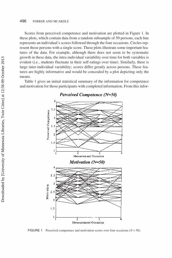
Scores from perceived competence and motivation are plotted in Figure 1. Inthese plots, which contain data from a random subsample of 50 persons, each linerepresents an individual’s scores followed through the four occasions. Circles rep-resent those persons with a single score. These plots illustrate some important fea-tures of the data. For example, although there does not seem to be systematicgrowth in these data, the intra-individual variability over time for both variables isevident (i.e., students fluctuate in their self-ratings over time). Similarly, there islarge inter-individual variability; scores differ greatly across persons. These fea-tures are highly informative and would be concealed by a plot depicting only themeans.

Table 1 gives an initial statistical summary of the information for competenceand motivation for those participants with completed information. From this infor-


FIGURE 1 Perceived competence and motivation scores over four occasions (N = 50).

Dow

nloa

ded

by [

Uni

vers

ity o

f M

inne

sota

Lib

rari

es, T

win

Citi

es]

at 1

2:56

09

Oct

ober

201

3

mation, one can observe a very small increase in both competence and motivationscores across occasions with greater variability in the competence scores. Simi-larly, one can observe high correlations among the competence scores and amongthe motivation scores, and moderate correlations between scores of both variables.No hints of autocorrelations are apparent for motivation or competence.

MODELS

Structural Cross-Lagged Regression Model

The initial model we use here is a structural cross-lagged longitudinal model. Thisclassical model is based on the pioneer work by Jöreskog (1970, 1974, 1979;Jöreskog & Sörbom, 1979) and is depicted as a path diagram in Figure 2.

This figure represents a system of two variables, X and Y, measured at four occa-sions. For each assessment, the observed scores, Y[t] and X[t] (squares), are a func-tion of true scores, y[t] and x[t], and measurement error, ey[t] and ex[t] (in circles), fol-lowing classical test theory, as

Y[t]n = y[t]n + ey[t]n and (1)

X[t]n = x[t]n + ex[t]n

Furthermore, this model specifies interrelations between the two variables atthe level of the true scores. Accordingly, each latent variable at time t is a functionof three components: (a) an autoregression (β), which represents the effect of thesame variable at a previous time and is constant across lags; (b) a cross-lagged re-gression (γ), or the effect of the other variable at a previous time, also constant


TABLE 1Summary Statistics for Competence and Motivation Across Four

Occasions

PC1 PC2 PC3 PC4 MO1 MO2 MO3 MO4

M 2.82 2.89 2.95 3.03 2.93 2.96 3.03 3.06SD .760 .677 .711 .706 .550 .555 .595 .614PC1 1.000PC2 0.778 1.000PC3 0.811 0.820 1.000PC4 0.791 0.758 0.853 1.000MO1 0.480 0.476 0.449 0.438 1.000MO2 0.394 0.496 0.360 0.399 0.619 1.000MO3 0.479 0.505 0.485 0.517 0.695 0.682 1.000MO4 0.504 0.468 0.457 0.561 0.632 0.712 0.786 1.000

Note. N = 144. PC = perceived competence; MO = motivation.

Dow

nloa

ded

by [

Uni

vers

ity o

f M

inne

sota

Lib

rari

es, T

win

Citi

es]

at 1

2:56

09

Oct

ober

201

3

across lags; and (c) a residual (d), allowed to correlate with the residual for theother variable at the same occasion and constrained to be equal across occasions.The equations of this model, without intercepts, can be written as

y[t]n = βy × y[t – 1]n + γy × x[t – 1]n + dy[t]n and (2)x[t]n = βx × x[t – 1]n + γx × y[t – 1]n + dx[t]n

According to these equations, the effects of the autoregression and cross-laggedregression parameters apply to the scores, not directly to the changes. However,this model can also be written as a set of first difference equations, as

∆y[t]n= βy × (∆y[t – 1]n) + γy × (∆x[t – 1]n) + ∆dy[t]n and (3)∆x[t]n= βx × (∆x[t – 1]n) + γx × (∆y[t – 1]n) + ∆dx[t]n


FIGURE 2 Path diagram of a bivariate cross-lagged regression model.

Dow

nloa

ded

by [

Uni

vers

ity o

f M

inne

sota

Lib

rari

es, T

win

Citi

es]

at 1

2:56

09

Oct

ober

201

3

where the changes in a variable are expressed as a function of changes in itself, rep-resented by the autoregressions (β) and changes in the other variable, representedby the cross-lagged regressions (γ). It can be seen from these equations that thecross-lagged model allows one to examine the interrelations between the two vari-ables over time but cannot capture the potential growth of the variables, as seen insubsequent models.

A Structural Factor Model Based on Latent Growth Curves

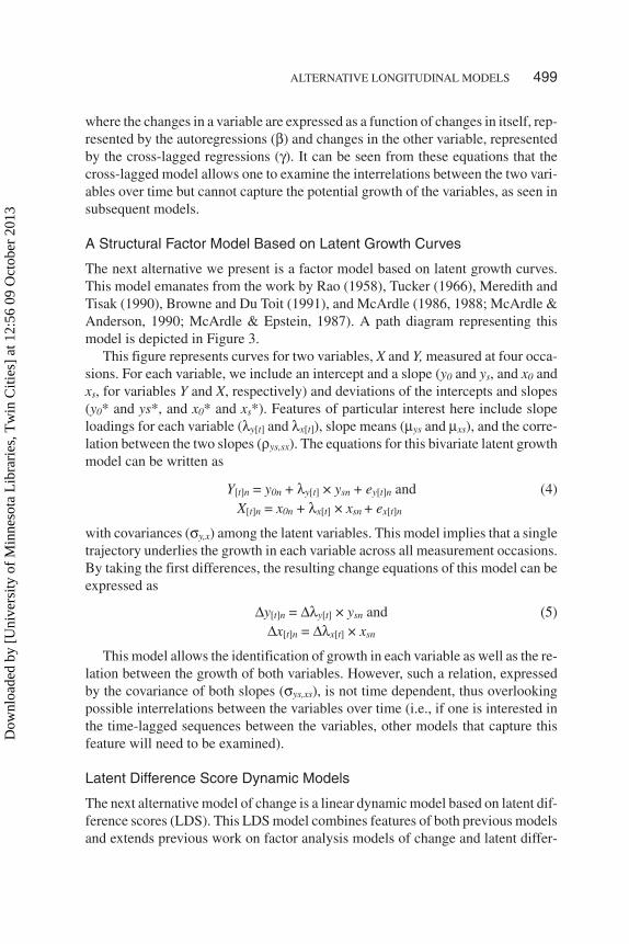
The next alternative we present is a factor model based on latent growth curves.This model emanates from the work by Rao (1958), Tucker (1966), Meredith andTisak (1990), Browne and Du Toit (1991), and McArdle (1986, 1988; McArdle &Anderson, 1990; McArdle & Epstein, 1987). A path diagram representing thismodel is depicted in Figure 3.

This figure represents curves for two variables, X and Y, measured at four occa-sions. For each variable, we include an intercept and a slope (y0 and ys, and x0 andxs, for variables Y and X, respectively) and deviations of the intercepts and slopes(y0* and ys*, and x0* and xs*). Features of particular interest here include slopeloadings for each variable (λy[t] and λx[t]), slope means (µys and µxs), and the corre-lation between the two slopes (ρys,sx). The equations for this bivariate latent growthmodel can be written as

Y[t]n = y0n + λy[t] × ysn + ey[t]n and (4)X[t]n = x0n + λx[t] × xsn + ex[t]n

with covariances (σy,x) among the latent variables. This model implies that a singletrajectory underlies the growth in each variable across all measurement occasions.By taking the first differences, the resulting change equations of this model can beexpressed as

∆y[t]n = ∆λy[t] × ysn and (5)∆x[t]n = ∆λx[t] × xsn

This model allows the identification of growth in each variable as well as the re-lation between the growth of both variables. However, such a relation, expressedby the covariance of both slopes (σys,xs), is not time dependent, thus overlookingpossible interrelations between the variables over time (i.e., if one is interested inthe time-lagged sequences between the variables, other models that capture thisfeature will need to be examined).

Latent Difference Score Dynamic Models

The next alternative model of change is a linear dynamic model based on latent dif-ference scores (LDS). This LDS model combines features of both previous modelsand extends previous work on factor analysis models of change and latent differ-


Dow

nloa

ded

by [

Uni

vers

ity o

f M

inne

sota

Lib

rari

es, T

win

Citi

es]

at 1

2:56

09

Oct

ober

201

3

500

FIGURE 3 Path diagram of a bivariate latent growth model.

Dow

nloa

ded

by [

Uni

vers

ity o

f M

inne

sota

Lib

rari

es, T

win

Citi

es]

at 1

2:56

09

Oct

ober

201

3

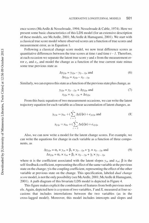
ence scores (McArdle & Nesselroade, 1994; Nesselroade & Cable, 1974). Here wepresent some basic characteristics of this LDS model (for an extensive descriptionof these models, see McArdle, 2001; McArdle & Hamagami, 2001). We start witha classical true score model where observed scores are a function of true scores andmeasurement error, as in Equation 1.

Following a classical change score model, we now treat difference scores asquantitative differences between the true scores at time t and time t – 1. Therefore,at each occasion we separate the latent true score y and x from the measurement er-ror ey and ex, and model the change as a function of the true current state minussome true previous state as

∆y[t]n = y[t]n – y[t – 1]n and (6)∆x[t]n = x[t]n – x[t – 1]n

Similarly,wecanexpress thisstateasafunctionof thepreviousstatepluschange,as

y[t]n = y[t – 1]n + ∆y[t]n and (7)x[t]n = x[t – 1]n + ∆x[t]n

From this basic equation of two measurement occasions, we can write the latenttrajectory equation for each variable as a linear accumulation of latent changes, as

Also, we can now write a model for the latent change scores. For example, wecan write the equations for change in each variable as a function of three compo-nents, as

∆y[t]n = αy × ysn + βy × y[t – 1]n + γy × x[t – 1]n and (9)∆x[t]n = αx × xsn + βx × x[t – 1]n + γx × y[t – 1]n

where α is the coefficient associated with the latent slopes ysn and xsn; β is theself-feedback coefficient, representing the effect of the same variable at the previousstate on the change; γ is the coupling coefficient, representing the effect of the othervariable at previous state on the change. This specification, labeled dual changescore model, is not the only possibility (see McArdle, 2001; McArdle & Hamagami,2001). A path diagram of this bivariate LDS model is depicted in Figure 4.

This figure makes explicit the combination of features from both previous mod-els. Again, depicted here is a system of two variables, Y and X, measured at four oc-casions that includes interrelations between the two variables (as in thecross-lagged model). Moreover, this model includes intercepts and slopes and


[ ] 0 [ ]1

[ ] 0 [ ]1

( [ ] ) and (8)

( [ ] )

t

t n n y t ni

t

t n n x t ni

y y y i n e

x x x i n e

∆

∆

�

�

� � �

� � �

�

�

Dow

nloa

ded

by [

Uni

vers

ity o

f M

inne

sota

Lib

rari

es, T

win

Citi

es]

at 1

2:56

09

Oct

ober

201

3

covariations among them (as in the latent growth curves model). A new feature ofthis LDS model, however, is a variable that represents change on each variable(∆y[t] and ∆x[t]). This variable of change is a latent component that is modeled, notobserved, and represents a key element of this LDS approach.

As represented in Figure 4 and Equation 9, the latent changes in the LDS modelare directly predicted from the levels of the variables at the previous occasion, withparametersβand γ representingsucheffects.Thisconceptualizationdiffers fromthecross-lagged regression model, where the change in one variable is predicted bychanges in itself andchanges in theothervariable (seeEquation3).Therefore, the in-terpretation of the β and γ parameters is different for both models. Furthermore, incontrast to the cross-lagged model, this specification of the LDS model is determin-istic and does not include a residual term. This difference sets the LDS model asidefrom Kessler and Greenberg’s (1981) specification of regression models in terms ofresidual change. However, both models can be written in terms of their change equa-tions. This approach has numerous merits (see Allison, 1990; Burr & Nesselroade,1990; Liker, Augustyniak, & Duncan, 1985; Nesselroade & Cable, 1974), and in theLDS method presented here, we model the scores directly but use a model that isbasedonaspecificconceptaboutchange (Coleman,1968; fora review, seeMcArdle& Nesselroade, 2003). In either case, the models in this article involve true scoresand more than two measurement occasions, thus avoiding some of the limitations oftwo-wave panel models (Kessler & Greenberg, 1981; Liker et al., 1985).

The LDS model relies on a series of assumptions, including (a) the effects of theLDS model apply directly to the true scores, and the effects on the observed scoresare only indirect; (b) the interval of time is discrete and known across measure-ments; (c) to simplify integration the LDS model is deterministic, although it couldbe extended to include stochastic components; and (d) the LDS accounts forinter-individual differences. Based on these assumptions, one can now test thisLDS model against alternative hypotheses of bivariate change using standardstructural equation modeling (SEM) techniques. For example, one can test thismodel against a model that includes coupling effects in one direction only (i.e.,from variable X to Y; γx = 0, γy ≠ 0; or vice versa) or not coupling effects (γx = 0, γy =0). Assuming multivariate normality, differences in the likelihood functionsamong these models follow a chi-square distribution so we can evaluate these dif-ferences in probabilistic terms.

RESULTS

Fit and Numerical Results From Alternative StructuralModels

In the following section, we present results from fitting the models to the data us-ing LISREL 8.5 (Jöreskog & Sörbom, 2001; identical results should be obtained


Dow

nloa

ded

by [

Uni

vers

ity o

f M

inne

sota

Lib

rari

es, T

win

Citi

es]

at 1

2:56

09

Oct

ober

201

3

503 FIGURE 4 Path diagram of a bivariate dynamic latent difference score.

Dow

nloa

ded

by [

Uni

vers

ity o

f M

inne

sota

Lib

rari

es, T

win

Citi

es]

at 1

2:56

09

Oct

ober

201

3

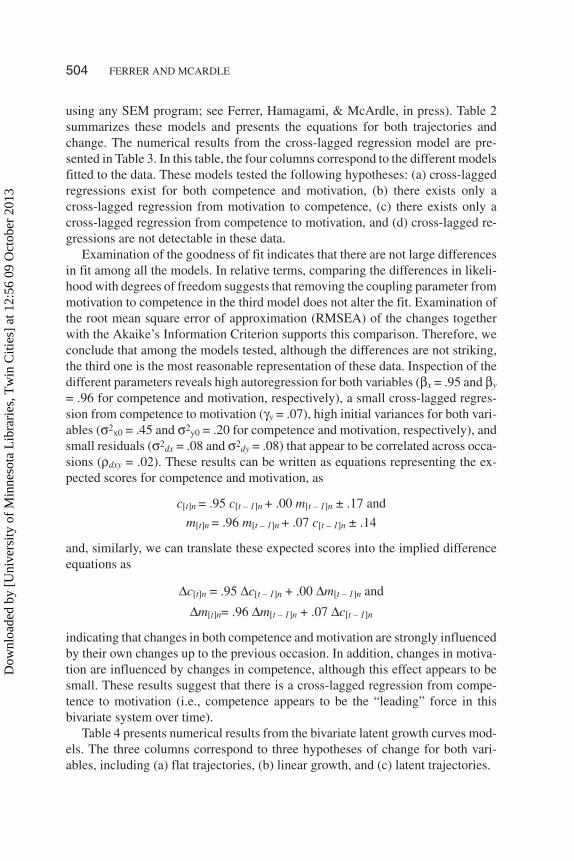
using any SEM program; see Ferrer, Hamagami, & McArdle, in press). Table 2summarizes these models and presents the equations for both trajectories andchange. The numerical results from the cross-lagged regression model are pre-sented in Table 3. In this table, the four columns correspond to the different modelsfitted to the data. These models tested the following hypotheses: (a) cross-laggedregressions exist for both competence and motivation, (b) there exists only across-lagged regression from motivation to competence, (c) there exists only across-lagged regression from competence to motivation, and (d) cross-lagged re-gressions are not detectable in these data.

Examination of the goodness of fit indicates that there are not large differencesin fit among all the models. In relative terms, comparing the differences in likeli-hood with degrees of freedom suggests that removing the coupling parameter frommotivation to competence in the third model does not alter the fit. Examination ofthe root mean square error of approximation (RMSEA) of the changes togetherwith the Akaike’s Information Criterion supports this comparison. Therefore, weconclude that among the models tested, although the differences are not striking,the third one is the most reasonable representation of these data. Inspection of thedifferent parameters reveals high autoregression for both variables (βx = .95 and βy

= .96 for competence and motivation, respectively), a small cross-lagged regres-sion from competence to motivation (γy = .07), high initial variances for both vari-ables (σ2x0 = .45 and σ2y0 = .20 for competence and motivation, respectively), andsmall residuals (σ2dx = .08 and σ2dy = .08) that appear to be correlated across occa-sions (ρdxy = .02). These results can be written as equations representing the ex-pected scores for competence and motivation, as

c[t]n = .95 c[t – 1]n + .00 m[t – 1]n ± .17 and

m[t]n = .96 m[t – 1]n + .07 c[t – 1]n ± .14

and, similarly, we can translate these expected scores into the implied differenceequations as

∆c[t]n = .95 ∆c[t – 1]n + .00 ∆m[t – 1]n and

∆m[t]n= .96 ∆m[t – 1]n + .07 ∆c[t – 1]n

indicating that changes in both competence and motivation are strongly influencedby their own changes up to the previous occasion. In addition, changes in motiva-tion are influenced by changes in competence, although this effect appears to besmall. These results suggest that there is a cross-lagged regression from compe-tence to motivation (i.e., competence appears to be the “leading” force in thisbivariate system over time).

Table 4 presents numerical results from the bivariate latent growth curves mod-els. The three columns correspond to three hypotheses of change for both vari-ables, including (a) flat trajectories, (b) linear growth, and (c) latent trajectories.


Dow

nloa

ded

by [

Uni

vers

ity o

f M

inne

sota

Lib

rari

es, T

win

Citi

es]

at 1

2:56

09

Oct

ober

201

3

505

TABLE 2Standard Algebraic Expressions of the Alternative Bivariate Models

Model Structural and Trajectory Equations Change Equationsa

Cross-lagged regression model y[t]n = βy · y[t – 1]n + γy · x[t – 1]n + dy[t]n ∆y[t]n = βy · (∆y[t – 1]n) + γy · (∆x[t – 1]n) + ∆dy[t]n

x[t]n = βx · x[t – 1]n + γx · y[t – 1]n + dx[t]n ∆x[t]n = βx · (∆x[t – 1]n) + γx · (∆y[t – 1]n) + ∆dx[t]n

Latent growth model Y[t]n = y0n + λy[t] · ysn + ey[t]n ∆y[t]n = ∆λy[t] · ysn

X[t]n = x0n + λx[t] · xsn + ex[t]n ∆x[t]n = ∆λx[t] · xsn

Latent difference score modely[t]n = y0n + ( ∆y i n e

i

t

y t n[ ] [ ]�

� �

1

) + ey[t]n∆y[t]n = αy · ysn + βy · y[t – 1]n + γy · x[t – 1]n

x[t]n = x0n + ( ∆x i n ei

t

x t n[ ] [ ]�

� �

1

) + ex[t]n∆x[t]n = αx · xsn + βx · x[t – 1]n + γx · y[t – 1]n

b

aChange equations here are first difference equations. bThese equations refer to a dual change model that includes the effects of both a slope (α) and feed for-ward (β).

Dow

nloa

ded

by [

Uni

vers

ity o

f M

inne

sota

Lib

rari

es, T

win

Citi

es]

at 1

2:56

09

Oct

ober

201

3

The first model specifies flat trajectories for both variables, thus estimatinginitial means and deviations but setting to zero all the slope components. Thismodel yields a relatively poor fit (L2 = 100, df = 37) but serves as a baseline toevaluate other models of growth. The second model (i.e., linear growth) includesslope components for both variables, and this results in a substantial improve-ment in fit (L2 = 44, df = 28; ∆χ2/∆df = 56/9; RMSEA ∆ = .19). Some importantparameter estimates of this model include initial mean levels (µc0 = 2.8 and µm0

= 2.9 for competence and motivation, respectively), level deviations (σc0 = .66and σm0 = .44), slope means (µcs = .21 and µms = .14), slope deviations (σcs = .22and σms = .24), a correlation between the intercepts (ρc0,m0 = .58), and an imper-ceptible correlation between the slopes (ρcs,ms ≈ 0). The last model specifies la-tent trajectories for both variables by freeing the slope loadings, but this does notimprove the fit from the linear model (L2 = 42, df = 24; ∆χ2/∆df = 2/4; RMSEA


TABLE 3Results From Cross-Lagged Bivariate Models for Perceived Competence and

Motivation

Parameters and FitIndexes

PC <=> MO MO => PC PC => MO No γ

PC MO PC MO PC MO PC MO

Regression coefficientsAutoregression β .94 (39) .97 (23) .92 (38) 1.0 (26) .95 (40) .96 (23) .94 (40) 1.0 (26)Cross-lag γ .03 (1) .07 (3) .05 (1) 0 (=) 0 (=) .07 (3) 0 (=) 0 (=)

Variancesσ2

0 .45 (7) .20 (3) .46 (7) .20 (6) .45 (7) .20 (6) .45 (7) .20 (6)σ2

d .03 (2) .03 (1) .03 (2) .02 (1) .03 (2) .03 (2) .03 (2) .02 (1)σ2

e .08 (15) .09 (16) .08 (7) .08 (8) .08 (7) .08 (7) .08 (7) .08 (8)ρdxy .02 (3) — .02 (3) — .02 (3) — .02 (3) —

Goodness of fitParameters 11 10 10 9Degrees of freedom 25 26 26 27Likelihood ratio L2 95 102 96 104RMSEA ea (p close fit) .13 (.00) .14 (.00) .13 (.00) .14 (.00)CFI .93 .92 .93 .92IFI .93 .92 .93 .92AIC 112 116 110 116

Fit changes∆χ2/∆df (RMSEA ∆1) — — 7/1 (.20) 1/1 (.00) 9/2 (.17)

6/0 (.19) 2/1 (.08)8/1 (.13)

Note. Numbers in parentheses by the parameter estimates represent t values. “1” RMSEA of the fit differ-ences. PC = perceived competence; MO = motivation; RMSEA = root mean square error of approximation; CFI =comparative fit index; IFI = Incremental Fit Index; AIC = Akaike’s Information Criterion.

Dow

nloa

ded

by [

Uni

vers

ity o

f M

inne

sota

Lib

rari

es, T

win

Citi

es]

at 1

2:56

09

Oct

ober

201

3

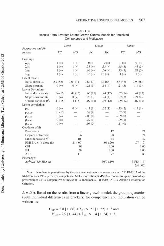
∆ = .00). Based on the results from a linear growth model, the group trajectories(with individual differences in brackets) for competence and motivation can bewritten as

C[t]n = 2.8 [± .66] + λc[t] × .21 [± .22] ± .3 andM[t]n= 2.9 [± .44] + λm[t] × .14 [± .24] ± .3.


TABLE 4Results From Bivariate Latent Growth Curves Models for Perceived

Competence and Motivation


Level Linear Latent

PC MO PC MO PC MO

Loadingsλ[1] 1 (=) 1 (=) 0 (=) 0 (=) 0 (=) 0 (=)λ[2] 1 (=) 1 (=) .33 (=) .33 (=) .45 (3) .43 (3)λ[3] 1 (=) 1 (=) .66 (=) .66 (=) .73 (5) .83 (5)λ[4] 1 (=) 1 (=) 1.0 (=) 1.0 (=) 1 (=) 1 (=)

Latent meansInitial mean µ0 2.9 (52) 3.0 (71) 2.8 (47) 2.9 (68) 2.8 (46) 2.9 (66)Slope mean µs 0 (=) 0 (=) .21 (5) .14 (4) .21 (5) .14 (3)

Latent DeviationsInitial deviation σ0 .64 (16) .48 (15) .66 (15) .44 (12) .67 (14) .44 (13)Slope deviation σs 0 (=) 0 (=) .22 (3) .24 (4) .22 (3) –.24 (4)Unique variance σ2

e .11 (15) .11 (15) .09 (12) .09 (12) .09 (12) .09 (12)Latent correlations

ρ0s 0 (=) 0 (=) –.13 (1) .22 (1) –.33 (2) –.17 (1)ρy0, x0 .61 (10) — .58 (8) — .57 (7) —ρy0, xs 0 (=) — –.06 (0) — –.09 (0) —ρys, x0 0 (=) — .29 (1) — –.29 (1) —ρys, xs 0 (=) — .07 (0) — .11 (0) —

Goodness of fitParameters 8 17 21Degrees of freedom 37 28 24Likelihood ratio L2 100 44 42RMSEA ea (p close fit) .11 (.00) .06 (.29) .07 (.17)CFI .99 1.00 1.00IFI .99 1.00 1.00AIC 118 77 83

Fit changes∆χ2/∆df (RMSEA ∆) — — 56/9 (.19) 58/13 (.16)

2/4 (.00)

Note. Numbers in parentheses by the parameter estimates represent t values. “1” RMSEA of thefit differences. PC = perceived competence; MO = motivation; RMSEA = root mean square error of ap-proximation; CFI = comparative fit index; IFI = Incremental Fit Index; AIC = Akaike’s InformationCriterion.

Dow

nloa

ded

by [

Uni

vers

ity o

f M

inne

sota

Lib

rari

es, T

win

Citi

es]

at 1

2:56

09

Oct

ober

201

3

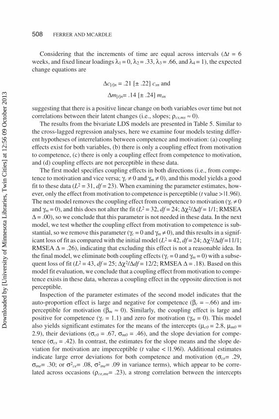
Considering that the increments of time are equal across intervals (∆t = 6weeks, and fixed linear loadings λ1 = 0, λ2 = .33, λ3 = .66, and λ4 = 1), the expectedchange equations are

∆c[t]n = .21 [± .22] csn and

∆m[t]n= .14 [± .24] msn

suggesting that there is a positive linear change on both variables over time but notcorrelations between their latent changes (i.e., slopes; ρcs,ms ≈ 0).

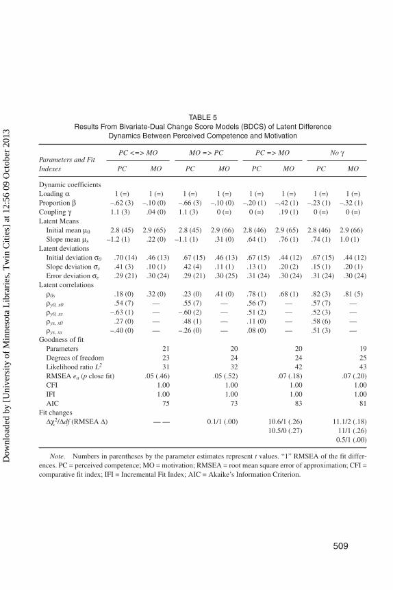
The results from the bivariate LDS models are presented in Table 5. Similar tothe cross-lagged regression analyses, here we examine four models testing differ-ent hypotheses of interrelations between competence and motivation: (a) couplingeffects exist for both variables, (b) there is only a coupling effect from motivationto competence, (c) there is only a coupling effect from competence to motivation,and (d) coupling effects are not perceptible in these data.

The first model specifies coupling effects in both directions (i.e., from compe-tence to motivation and vice versa; γc ≠ 0 and γm ≠ 0), and this model yields a goodfit to these data (L2 = 31, df = 23). When examining the parameter estimates, how-ever, only the effect from motivation to competence is perceptible (t value > |1.96|).The next model removes the coupling effect from competence to motivation (γc ≠ 0and γm = 0), and this does not alter the fit (L2 = 32, df = 24; ∆χ2/∆df = 1/1; RMSEA∆ = .00), so we conclude that this parameter is not needed in these data. In the nextmodel, we test whether the coupling effect from motivation to competence is sub-stantial, so we remove this parameter (γc = 0 and γm ≠ 0), and this results in a signif-icant loss of fit as compared with the initial model (L2 = 42, df = 24; ∆χ2/∆df =11/1;RMSEA ∆ = .26), indicating that excluding this effect is not a reasonable idea. Inthe final model, we eliminate both coupling effects (γc = 0 and γm = 0) with a subse-quent loss of fit (L2 = 43, df = 25; ∆χ2/∆df = 12/2; RMSEA ∆ = .18). Based on thismodel fit evaluation, we conclude that a coupling effect from motivation to compe-tence exists in these data, whereas a coupling effect in the opposite direction is notperceptible.

Inspection of the parameter estimates of the second model indicates that theauto-proportion effect is large and negative for competence (βc = –.66) and im-perceptible for motivation (βm ≈ 0). Similarly, the coupling effect is large andpositive for competence (γc = 1.1) and zero for motivation (γm = 0). This modelalso yields significant estimates for the means of the intercepts (µc0 = 2.8, µm0 =2.9), their deviations (σc0 = .67, σm0 = .46), and the slope deviation for compe-tence (σcs = .42). In contrast, the estimates for the slope means and the slope de-viation for motivation are imperceptible (t value < |1.96|). Additional estimatesindicate large error deviations for both competence and motivation (σce= .29,σme= .30; or σ2ce= .08, σ2me= .09 in variance terms), which appear to be corre-lated across occasions (ρce,me= .23), a strong correlation between the intercepts


Dow

nloa

ded

by [

Uni

vers

ity o

f M

inne

sota

Lib

rari

es, T

win

Citi

es]

at 1

2:56

09

Oct

ober

201

3

509

TABLE 5Results From Bivariate-Dual Change Score Models (BDCS) of Latent Difference

Dynamics Between Perceived Competence and Motivation


PC <=> MO MO => PC PC => MO No γ

PC MO PC MO PC MO PC MO

Dynamic coefficientsLoading α 1 (=) 1 (=) 1 (=) 1 (=) 1 (=) 1 (=) 1 (=) 1 (=)Proportion β –.62 (3) –.10 (0) –.66 (3) –.10 (0) –.20 (1) –.42 (1) –.23 (1) –.32 (1)Coupling γ 1.1 (3) .04 (0) 1.1 (3) 0 (=) 0 (=) .19 (1) 0 (=) 0 (=)Latent Means

Initial mean µ0 2.8 (45) 2.9 (65) 2.8 (45) 2.9 (66) 2.8 (46) 2.9 (65) 2.8 (46) 2.9 (66)Slope mean µs –1.2 (1) .22 (0) –1.1 (1) .31 (0) .64 (1) .76 (1) .74 (1) 1.0 (1)

Latent deviationsInitial deviation σ0 .70 (14) .46 (13) .67 (15) .46 (13) .67 (15) .44 (12) .67 (15) .44 (12)Slope deviation σs .41 (3) .10 (1) .42 (4) .11 (1) .13 (1) .20 (2) .15 (1) .20 (1)Error deviation σe .29 (21) .30 (24) .29 (21) .30 (25) .31 (24) .30 (24) .31 (24) .30 (24)

Latent correlationsρ0s .18 (0) .32 (0) .23 (0) .41 (0) .78 (1) .68 (1) .82 (3) .81 (5)ρy0, x0 .54 (7) — .55 (7) — .56 (7) — .57 (7) —ρy0, xs –.63 (1) — –.60 (2) — .51 (2) — .52 (3) —ρys, x0 .27 (0) — .48 (1) — .11 (0) — .58 (6) —ρys, xs –.40 (0) — –.26 (0) — .08 (0) — .51 (3) —

Goodness of fitParameters 21 20 20 19Degrees of freedom 23 24 24 25Likelihood ratio L2 31 32 42 43RMSEA ea (p close fit) .05 (.46) .05 (.52) .07 (.18) .07 (.20)CFI 1.00 1.00 1.00 1.00IFI 1.00 1.00 1.00 1.00AIC 75 73 83 81

Fit changes∆χ2/∆df (RMSEA ∆) — — 0.1/1 (.00) 10.6/1 (.26) 11.1/2 (.18)

10.5/0 (.27) 11/1 (.26)0.5/1 (.00)

Note. Numbers in parentheses by the parameter estimates represent t values. “1” RMSEA of the fit differ-ences. PC = perceived competence; MO = motivation; RMSEA = root mean square error of approximation; CFI =comparative fit index; IFI = Incremental Fit Index; AIC = Akaike’s Information Criterion.

Dow

nloa

ded

by [

Uni

vers

ity o

f M

inne

sota

Lib

rari

es, T

win

Citi

es]

at 1

2:56

09

Oct

ober

201

3

of both variables (ρc0,m0 = .55), and an imperceptible correlation between theslopes (ρcs,ms ≈ 0). Based on these results, we can write the group trajectories(with individual differences in brackets) for competence and motivation as

and the equations of the latent change scores as

∆c[t]n = 0 [± .42] csn –.66 c[t – 1]n + 1.10 m[t – 1]n and

∆m[t]n = 0 [± .00] msn +.00 m[t – 1]n + .00 c[t – 1]n

A plot of expected latent trajectories, free from measurement error, for eachvariable based on these results is depicted in Figure 5. In this plot, we combine in-dividual trajectories for N = 20 random individuals with the grand mean (thickline). For motivation, the figure suggests a collection of flat trajectories with verylittle variability in the initial level across persons. For competence, in contrast, thefigure depicts a linear growth with apparent variability in both the initial level andthe slope across individuals.

The plots in Figure 5 represent the expected mean trajectories for each variablein the bivariate system as a function of both itself and the other variable. Such tra-jectories will be different depending on the initial scores of both variables. This in-terplay between the variables’ starting point and the resulting trajectories is de-picted in Figures 6a and 6b. Here, the expected mean for each variable is plotted asa function of three different initial values of itself (i.e., 1.96 SD above the mean,overall mean, and 1.96 SD below the mean). Moreover, for each of these condi-tions three lines are included that represent the trajectory of the variable as a func-tion of different initial values for the other variable (i.e., +1.96 SD, mean, –1.96SD). This plot illustrates how the initial conditions alter the expected trajectoriesfor the variable in each bivariate system.

The expected trajectories for motivation are displayed in Figure 6a. Given thelack of coupling from competence to motivation, these trajectories are not affectedby initial scores in competence. Moreover, because of the negligible influencesfrom itself and slope, all the trajectories are flat, regardless of the initial score. Forcompetence (see Figure 6b), however, the dependence of the trajectories on initialscores is apparent. For average and low initial values of itself, competence scoresincrease over time, and this is more pronounced under conditions of higher initialscores on motivation. Only for higher initial values on itself, competence valuesdecrease over time, perhaps due to a ceiling effect.


[ ]1

[ ]1

2.8[ .67] ( [ ] ) .29 and

2.9[ .46] ( [ ] ) .30

t

t ni

t

t ni

c c i n

m m i n

∆

∆

�

�

� � � �

� � � �

�

�

Dow

nloa

ded

by [

Uni

vers

ity o

f M

inne

sota

Lib

rari

es, T

win

Citi

es]

at 1

2:56

09

Oct

ober

201

3

An alternative way to display these dynamic relations is using a vector field(Boker & McArdle, 1995). Figure 7 presents such a vector field together with anellipsoid containing 95% of the data to highlight where the changes are expected tooccur. In this plot, each arrow represents the expected direction of change for a pairof scores within that specific area of the plane. For example, given a pair of latentscores at a time t (i.e., c[t] = 3, m[t] = 3.5), this vector field forecasts an increase incompetence scores the next occasion of measurement (i.e., t + 1) but no changes inmotivation, and this dynamic influence is expected to be stronger for higher valuesof motivation. Therefore, according to these results, motivation appears to be aleading indicator in the system of interrelations between competence and motiva-tion over time.

DISCUSSION

In this study we applied alternative methods to examine the dynamics of adoles-cents’ competence and motivation during their first semester in high school. We


FIGURE 5 Expected latent trajectories for motivation and competence.

Dow

nloa

ded

by [

Uni

vers

ity o

f M

inne

sota

Lib

rari

es, T

win

Citi

es]

at 1

2:56

09

Oct

ober

201

3

analyzed these longitudinal data using three different methods, which, in turn,yielded different results. These contradictory findings are the result of applyingtechniques with different underlying models of change. Such contrasting findingssuggest that the researchers’ underlying theory of change should drive the selec-tion of methodology. In this study, the LDS models appear to be reasonable forthese data because they allow examination of the dynamics of two variables and, at


FIGURE 6 Expected latent trajectories for motivation (top) and competence (bottom) as afunction of the competence motivation system.

Dow

nloa

ded

by [

Uni

vers

ity o

f M

inne

sota

Lib

rari

es, T

win

Citi

es]

at 1

2:56

09

Oct

ober

201

3

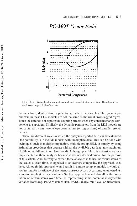
the same time, identification of potential growth in the variables. The dynamic pa-rameters in these LDS models are not the same as the usual cross-lagged regres-sions; the latter do not capture the coupling effects when any constant change com-ponents are apparent. Similarly, the dynamic parameters from the LDS models arenot captured by any level–slope correlations (or regressions) of parallel growthcurves.

There are different ways in which the analyses reported here can be extended.One possibility is to include models with incomplete data. This can be done withtechniques such as multiple imputation, multiple group SEM, or simply by usingestimation procedures that operate with all the available data (e.g., raw maximumlikelihood or full maximum likelihood). Although possible, this extension was notimplemented in these analyses because it was not deemed crucial for the purposeof this article. Another way to extend these analyses is to use individual items ofthe scales at each time, as opposed to an average composite, the approach usedhere. Although this approach would result in a more complex model, it would al-low testing for invariance of the latent construct across occasions, an untested as-sumption implicit in these analyses. Such an approach would also allow the corre-lation of certain items over time, as representing some potential idiosyncraticvariance (Jöreskog, 1979; Marsh & Hau, 1996). Finally, multilevel or hierarchical


FIGURE 7 Vector field of competence and motivation latent scores. Note. The ellipsoid isused to encompass 95% of the data.

Dow

nloa

ded

by [

Uni

vers

ity o

f M

inne

sota

Lib

rari

es, T

win

Citi

es]

at 1

2:56

09

Oct

ober

201

3

linear models could also be applied to these data. This approach would be particu-larly useful when the data are structured in clusters (e.g., students within classes)or unbalanced (i.e., the spacing between assessments is different among individu-als). These conditions, however, were not manifest in the data analyzed here. Stu-dents in this study were drawn from seven different classes only, and thus, the clus-tering effect was not deemed important. Furthermore, the spacing betweenobservations was approximately equal for all participants. Because these two con-ditions were not apparent, we did not consider using hierarchical linear models.

Substantively, our findings from the LDS models suggest that, for this sampleof students, motivation was the leading indicator of changes in competence overtime. That is, as these students moved through their first 6 months in high school,motivation appeared to be the force driving their changes in perceived competence.A plausible interpretation of these findings is that choosing challenging activities,putting forth effort in the tasks, and persisting in the face of failures led students toincrease practice, which, in turn, led to a more positive perceived ability. Thesefindings depart from theoretical contentions that propose relations from perceivedcompetence to intrinsic motivation (Deci & Ryan, 1985, 1991; Harter, 1987, 1990,1998; Vallerand, 1997). They also depart from empirical attempts to untangledirectionality between both constructs. In one of these attempts, Losier andVallerand (1994) used a two-wave, cross-lagged regression analysis and claimedthat perceived competence at Time 1 predicted motivation at Time 2, whereas mo-tivation at Time 1 did not predict perceived competence at Time 2. Such results,however, were negligible (p < .11), and the study involved only two occasions ofmeasurement over a 5-month period.

These findings are consistent with research indicating a reversed directionalitybetween perceived competence and motivation. For example, Boggiano (1998)suggested that intrinsic motivation may lead to perceived competence and can me-diate or moderate the effects of individuals’ autonomy on competence. Boggianofound supporting evidence for a relation in which motivation leads to competence(Boggiano, 1998; Guay, Boggiano, & Vallerand, 2001). Although both studies in-volved only two data points, they yielded consistent results and, furthermore, theyshowed that a relation of motivation leading to competence was more likely thanthe opposite. Additional studies using longitudinal data with alternative modelsapplied in different domains are needed to further examine the relation betweencompetence and motivation over time before a more definitive statement regardingdirectionality of effects can be made.

In this study, we analyzed the same longitudinal data using three alternativemethods. Each yielded different results. We indicated the necessity of defining atheory of change to help select which method is used to analyze the data. For thesedata, we concluded that LDS models were the most reasonable method becausethey capture dynamic interrelations between the variables and, at the same time,identify potential growth in the variables.


Dow

nloa

ded

by [

Uni

vers

ity o

f M

inne

sota

Lib

rari

es, T

win

Citi

es]

at 1

2:56

09

Oct

ober

201

3

ACKNOWLEDGMENTS

Support for preparation of this article was provided by Grant T32 AG20500-01from the National Institute on Aging.

These analyses were presented at the Biennial of the Society for Research inChild Development, Minneapolis, MN, April 2001.

We thank our colleague, Fumiaki Hamagami, for his help and commentsthroughout this research.

REFERENCES

Allison, P. D. (1990). Change scores as dependent variables in regression analysis. In C. C. Clogg (Ed.),Sociological methodology (pp. 93–114). San Francisco: Jossey-Bass.

Bijleveld, C. C. J. H., van der Kamp L. J. T., Mooijaart, A., van der Kloot, W. A., van der Leeden, R., &van der Burg, E. (1998). Longitudinal data analysis: Designs, models, and methods. London: Sage.

Boggiano, A. K. (1998). Maladaptive achievement patterns: A test of a diathesis-stress analysis of help-lessness. Journal of Personality and Social Psychology, 74, 1681–1695.

Boker S. M., & McArdle, J. J. (1995). Statistical vector field analysis applied to mixed cross-sectionaland longitudinal data. Experimental Aging Research, 21, 77–93.

Browne, M., & Du Toit, S. H. C. (1991). Models for learning data. In L. Collins & J. L. Horn (Eds.),Best methods for the analysis of change (pp. 47–68). Washington, DC: American PsychologicalAssociation.

Burr, J. A., & Nesselroade, J. R. (1990). Change measurement. In A. von Eye (Ed.), Statistical methodsin longitudinal research (pp. 3–34). New York: Academic.

Coleman, J. S. (1968). The mathematical study of change. In H. M. Blalock & A. B. Blalock (Eds.),Methodology in social research (pp. 428–478). New York: McGraw-Hill.

Collins, L. M., & Horn, J. L. (Eds.). (1991). Best methods for the analysis of change. Washington, DC:American Psychological Association.

Collins, L. M., & Sayer, A. (Eds.). (2001). New methods for the analysis of change. Washington, DC:American Psychological Association.

Deci, E. L., & Ryan, R. M. (1985). Intrinsic motivation and self-determination in human behavior. NewYork: Plenum.

Deci, E. L., & Ryan, R. M. (1991). A motivational approach to self: Integration in personality. In R.Dienstbier (Ed.), Nebraska symposium on motivation: Vol. 38: Perspectives on motivation (pp.237–288). Lincoln: University of Nebraska Press.

Deci, E. L., Vallerand, R. J., Pelletier, L. G., & Ryan, R. M. (1991). Motivation and education: Theself-determination perspective. Educational Psychologist, 26, 325–346.

Ferrer, E., Hamagami, F., & McArdle, J. J. (in press). Modeling latent growth curves with incompletedata using different types of structural equation modeling and multilevel software. Structural Equa-tion Modeling.

Ferrer-Caja, E., & Weiss, M. R. (2000). Predictors of intrinsic motivation among adolescent students inphysical education. Research Quarterly for Exercise and Sport, 71, 267–279.

Ferrer-Caja, E., & Weiss, M. R. (2002). Cross-validation of a model of intrinsic motivation in highschool with students in elective courses. Journal of Experimental Education, 71, 41–65.

Guay, F., Boggiano, A. K., & Vallerand, R. J. (2001). Autonomy support, intrinsic motivation, and per-ceived competence: Conceptual and empirical linkages. Personality and Social Psychology Bulletin,27, 643–650.


Dow

nloa

ded

by [

Uni

vers

ity o

f M

inne

sota

Lib

rari

es, T

win

Citi

es]

at 1

2:56

09

Oct

ober

201

3

Harter, S. (1987). The determinants and mediational role of global self-worth in children. In N.Eisenberg (Ed.), Contemporary issues in developmental psychology (pp. 219–242). New York:Wiley.

Harter, S. (1988). The self-perception profile for adolescents. Unpublished manual, University of Den-ver, CO.

Harter, S. (1990). Adolescent self and identity development. In S. S. Feldman & G. R. Elliot (Eds.), At thethreshold: The developing adolescent (pp. 352–387). Cambridge, MA: Harvard University Press.

Harter, S. (1998). The development of self-representations. In N. Eisenberg (Ed.), Handbook of childpsychology: Volume 3, Social, emotional, and personality development (pp. 553–618). New York:Wiley.

Harter, S. (1999). The construction of the self. New York: Guilford.Jöreskog, K. G. (1970). Estimation and testing of simplex models. British Journal of Mathematical and

Statistical Psychology, 23, 121–145.Jöreskog, K. G. (1974). Analyzing psychological data by structural analysis of covariance matrices. In

R. C. Atkinson, D. H. Krantz, R. D. Luce, & P. Suppas (Eds.), Contemporary developments in mathe-matical psychology (pp. 1–56). San Francisco: Freeman.

Jöreskog, K. G. (1979). Statistical estimation of structural models in longitudinal–developmental in-vestigations. In J. R. Nesselroade & P. B. Baltes (Eds.), Longitudinal research in the study of behav-ior and development (pp. 303–352). New York: Academic.

Jöreskog, K. G., & Sörbom, D. (1979). Advances in factor analysis and structural equation models.Cambridge, MA: Abt Books.

Jöreskog, K. G., & Sörbom, D. (2001). LISREL (Version 8.5) [Computer software]. Chicago: ScientificSoftware International.

Kessler, R. C., & Greenberg, D. F. (1981). Linear panel analysis: Models of quantitative change. NewYork: Academic.

Liker, J. K., Augustyniak, S., & Duncan, G. J. (1985). Panel data and models of change: A comparisonof first difference and conventional two-wave models. Social Science Research, 14, 80–101.

Little, T. D., Schnabel, K. U., & Baumert, J. (Eds.). (2000). Modeling longitudinal and multiple-groupdata: Practical issues, applied approaches, and scientific examples. Mahwah, NJ: LawrenceErlbaum Associates, Inc.

Losier, G. A., & Vallerand, R. J. (1994). The temporal relationship between perceived competence andself-determined motivation. Journal of Social Psychology, 134, 793–801.

Marsh, H. W., & Hau, K. T. (1996). Assessing goodness of fit: Is parsimony always desirable? Journalof Experimental Education, 64, 364–390.

McArdle, J. J. (1986). Latent variable growth within behavior genetic models. Behavior Genetics, 16,163–200.

McArdle, J. J. (1988). Dynamic but structural equation modeling of repeated measures data. In J. R.Nesselroade & R. B. Cattell (Eds.), The handbook of multivariate experimental psychology, Volume2 (pp. 561–614). New York: Plenum.

McArdle, J. J. (2001). A latent difference score approach to longitudinal dynamic analysis. In R.Cudeck, S. Du Toit, & D. Sörbom (Eds.), Structural equation modeling: Present and future (pp.341–380). Lincolnwood, IL: Scientific Software International.

McArdle, J. J., & Anderson, E. (1990). Latent variable growth models for research on aging. In J. E.Birren & K. W. Schaie (Eds.), The handbook of the psychology of aging (pp. 21–43). New York: Ple-num.

McArdle, J. J., & Epstein, D. B. (1987). Latent growth curves within developmental structural equationmodels. Child Development, 58, 110–133.

McArdle, J. J., & Hamagami, F. (2001). Latent difference score structural models for linear dynamicanalyses with incomplete longitudinal data. In L. Collins & A. Sayer (Eds.), New methods for theanalysis of change (pp. 139–175). Washington, DC: American Psychological Association.


Dow

nloa

ded

by [

Uni

vers

ity o

f M

inne

sota

Lib

rari

es, T

win

Citi

es]

at 1

2:56

09

Oct

ober

201

3

McArdle, J. J., & Nesselroade, J. R. (1994). Structuring data to study development and change. In S. H.Cohen & H. W. Reese (Eds.), Life-span developmental psychology: Methodological innovations (pp.223–267). Hillsdale, NJ: Lawrence Erlbaum Associates, Inc.

McArdle, J. J., & Nesselroade, J. R. (2003). Growth curve analysis in contemporary research. In J.Schinka & W. Velicer (Eds.), Comprehensive handbook of psychology, Vol. II: Research methods inpsychology (pp. 447–480). New York: Pergamon.

Meredith, W., & Tisak, J. (1990). Latent curve analysis. Psychometrika, 55, 107–122.Moskowitz, D. M., & Hershberger, S. L. (2002). Modeling intraindividual variability with repeated

measures data: Advances and techniques. Mahwah, NJ: Lawrence Erlbaum Associates, Inc.Nesselroade, J. R., & Cable, D. G. (1974). Sometimes it’s okay to factor difference scores—The separa-

tion of state and trait anxiety. Multivariate Behavioral Research, 9, 273–282.Rao, C. R. (1958). Some statistical methods for the comparison of growth curves. Biometrics, 14, 1–17.Stinnett, T. A., Oehler-Stinnett, J., & Stout, L. J. (1991). Development of the teacher rating of academic

achievement motivation: TRAAM. School Psychology Review, 20, 609–622.Tucker, L. R. (1966). Learning theory and multivariate experiment: Illustration by determination of pa-

rameters of generalized learning curves. In R. B. Cattell (Ed.), The handbook of multivariate experi-mental psychology (pp. 476–501). Chicago: Rand McNally.

Vallerand, R. J. (1997). Toward a hierarchical model of intrinsic and extrinsic motivation. In M. P.Zanna (Ed.), Advances in experimental social psychology (Vol. 29, pp. 271–360). New York: Aca-demic.

von Eye, A. (Ed.). (1990). Statistical methods in longitudinal research. New York: Academic.

APPENDIX ALISREL Input File for a Cross-Lagged Regression Model

BIVARIATE ANALYSIS OF COMPETENCE AND MOTIVATION!Cross-Lagged Regression Model (Y=MOT; X=PC)!Model1: Full “Coupling”DA NO=144 NI=9 MA=CMLA FI=pc_mot.datME FI=pc_mot.datSD FI=pc_mot.datKM SY FI=pc_mot.datSElectmot1 mot2 mot3 mot4 pc1 pc2 pc3 pc4 /MO NY=8 NE=24 LY=FI,FU BE=FI,FU PS=FI,SY TE=ZELEY[0] Y[1] Y[2] Y[3]e[0] e[1] e[2] e[3]y[0] y[1] y[2] y[3]X[0] X[1] X[2] X[3]f[0] f[1] f[2] f[3]x[0] x[1] x[2] x[3]!*****************************************


Dow

nloa

ded

by [

Uni

vers

ity o

f M

inne

sota

Lib

rari

es, T

win

Citi

es]

at 1

2:56

09

Oct

ober

201

3

!Model for the Y variables!*****************************************!FILTERST 1 LY(1,1) LY(2,2) LY(3,3) LY(4,4)!ERRORSFR BE(1,5) BE(2,6) BE(3,7) BE(4,8)EQ BE(1,5) BE(2,6) BE(3,7) BE(4,8)ST .3 BE(1,5) BE(2,6) BE(3,7) BE(4,8)!ST 0 BE(1,5) BE(2,6) BE(3,7) BE(4,8)ST 1 PS(5,5) PS(6,6) PS(7,7) PS(8,8)!MEASUREMENTST 1 BE(1,9) BE(2,10) BE(3,11) BE(4,12)!AUTOREGRESSION BETAFR BE(10,9) BE(11,10) BE(12,11)ST .1 BE(10,9) BE(11,10) BE(12,11)EQ BE(10,9) BE(11,10) BE(12,11)!VARIANCESFR PS(9,9)ST 1 PS(9,9)!RESIDUALSFR PS(10,10) PS(11,11) PS(12,12)ST 1 PS(10,10) PS(11,11) PS(12,12)EQ PS(10,10) PS(11,11) PS(12,12)!*****************************************!Model for the X variables!*****************************************ST 1 LY(5,13) LY(6,14) LY(7,15) LY(8,16)!ERRORSFR BE(13,17) BE(14,18) BE(15,19) BE(16,20)EQ BE(13,17) BE(14,18) BE(15,19) BE(16,20)ST .3 BE(13,17) BE(14,18) BE(15,19) BE(16,20)!ST 0 BE(13,17) BE(14,18) BE(15,19) BE(16,20)ST 1 PS(17,17) PS(18,18) PS(19,19) PS(20,20)!MEASUREMENTST 1 BE(13,21) BE(14,22) BE(15,23) BE(16,24)!AUTOREGRESSION BETAFR BE(22,21) BE(23,22) BE(24,23)ST .1 BE(22,21) BE(23,22) BE(24,23)EQ BE(22,21) BE(23,22) BE(24,23)!VARIANCESFR PS(21,21)ST 1 PS(21,21)


Dow

nloa

ded

by [

Uni

vers

ity o

f M

inne

sota

Lib

rari

es, T

win

Citi

es]

at 1

2:56

09

Oct

ober

201

3

!RESIDUALSFR PS(22,22) PS(23,23) PS(24,24)ST 1 PS(22,22) PS(23,23) PS(24,24)EQ PS(22,22) PS(23,23) PS(24,24)!*****************************************!Model for the yX relations!*****************************************!UNIQUE CORRELATIONS!FR PS(17,5) PS(18,6) PS(19,7) PS(20,8)!EQ PS(17,5) PS(18,6) PS(19,7) PS(20,8)!ST .001 PS(17,5) PS(18,6) PS(19,7) PS(20,8)!RESIDUALS CORRELATIONSFR PS(10,22) PS(11,23) PS(12,24)EQ PS(10,22) PS(11,23) PS(12,24)ST .01 PS(10,22) PS(11,23) PS(12,24)!CROSSLAG REGRESSION Dx<LyFR BE(22,9) BE(23,10) BE(24,11)EQ BE(22,9) BE(23,10) BE(24,11)ST .1 BE(22,9) BE(23,10) BE(24,11)!CROSSLAG REGRESSION Dy<LxFR BE(10,21) BE(11,22) BE(12,23)EQ BE(10,21) BE(11,22) BE(12,23)ST .1 BE(10,21) BE(11,22) BE(12,23)OU NS ML IT=100 AD=OF XM ND=2

APPENDIX BLISREL Input File for a Latent Growth Model

BIVARIATE ANALYSIS OF COMPETENCE AND MOTIVATION!Latent Growth Curve Model (Y=MOT; X=PC)!Model3: Latent GrowthDA NO=144 NI=9 MA=MMLA FI=pc_mot.datME FI=pc_mot.datSD FI=pc_mot.datKM SY FI=pc_mot.datSEmot1 mot2 mot3 mot4 pc1 pc2 pc3 pc4 K /MO NY=9 NE=25 LY=FI,FU BE=FI,FU PS=FI,SY TE=ZELEY[0] Y[1] Y[2] Y[3]


Dow

nloa

ded

by [

Uni

vers

ity o

f M

inne

sota

Lib

rari

es, T

win

Citi

es]

at 1

2:56

09

Oct

ober

201

3

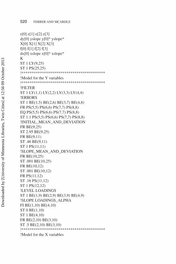
e[0] e[1] e[2] e[3]dy[0] yslope y[0]* yslope*X[0] X[1] X[2] X[3]f[0] f[1] f[2] f[3]dx[0] xslope x[0]* xslope*KST 1 LY(9,25)ST 1 PS(25,25)!*****************************************!Model for the Y variables!*****************************************!FILTERST 1 LY(1,1) LY(2,2) LY(3,3) LY(4,4)!ERRORSST 1 BE(1,5) BE(2,6) BE(3,7) BE(4,8)FR PS(5,5) PS(6,6) PS(7,7) PS(8,8)EQ PS(5,5) PS(6,6) PS(7,7) PS(8,8)ST 1.1 PS(5,5) PS(6,6) PS(7,7) PS(8,8)!INITIAL_MEAN_AND_DEVIATIONFR BE(9,25)ST 2.95 BE(9,25)FR BE(9,11)ST .46 BE(9,11)ST 1 PS(11,11)!SLOPE_MEAN_AND_DEVIATIONFR BE(10,25)ST .001 BE(10,25)FR BE(10,12)ST .001 BE(10,12)FR PS(11,12)ST .16 PS(11,12)ST 1 PS(12,12)!LEVEL LOADINGSST 1 BE(1,9) BE(2,9) BE(3,9) BE(4,9)!SLOPE LOADINGS_ALPHAFI BE(1,10) BE(4,10)ST 0 BE(1,10)ST 1 BE(4,10)FR BE(2,10) BE(3,10)ST .5 BE(2,10) BE(3,10)!*****************************************!Model for the X variables


Dow

nloa

ded

by [

Uni

vers

ity o

f M

inne

sota

Lib

rari

es, T

win

Citi

es]

at 1

2:56

09

Oct

ober

201

3

!*****************************************ST 1 LY(5,13) LY(6,14) LY(7,15) LY(8,16)!ERRORSST 1 BE(13,17) BE(14,18) BE(15,19) BE(16,20)FR PS(17,17) PS(18,18) PS(19,19) PS(20,20)EQ PS(17,17) PS(18,18) PS(19,19) PS(20,20)ST 1.1 PS(17,17) PS(18,18) PS(19,19) PS(20,20)!INITIAL_MEAN_AND_DEVIATIONFR BE(21,25)ST 3 BE(21,25)FR BE(21,23)ST .62 BE(21,23)ST 1 PS(23,23)!SLOPE_MEAN_AND_DEVIATIONFR BE(22,25)ST .001 BE(22,25)FR BE(22,24)ST .24 BE(22,24)FR PS(23,24)ST .1 PS(23,24)ST 1 PS(24,24)!LEVEL LOADINGSST 1 BE(13,21) BE(14,21) BE(15,21) BE(16,21)!SLOPE LOADINGS_ALPHAFI BE(13,22) BE(16,22)ST 0 BE(13,22)ST 1 BE(16,22)FR BE(14,22) BE(15,22)ST .5 BE(14,22) BE(15,22)!*****************************************!Model for the yX relations!*****************************************!LEVEL AND SLOPE CORRELATIONSFR PS(11,23) PS(11,24) PS(12,23) PS(12,24)ST .01 PS(11,24) PS(12,23) PS(12,24)ST .5 PS(11,23)!UNIQUE CORRELATIONSFR PS(5,17) PS(6,18) PS(7,19) PS(8,20)EQ PS(5,17) PS(6,18) PS(7,19) PS(8,20)ST .03 PS(5,17) PS(6,18) PS(7,19) PS(8,20)OU NS ML IT=100 AD=OFf XM ND=2


Dow

nloa

ded

by [

Uni

vers

ity o

f M

inne

sota

Lib

rari

es, T

win

Citi

es]

at 1

2:56

09

Oct

ober

201

3

APPENDIX CLISREL Input File for Dynamic Latent Difference Score

Model

BIVARIATE ANALYSIS OF COMPETENCE AND MOTIVATION!Latent Difference Score Model (Y=MOT; X=PC)!Model1: Full “Coupling”DAta NObservations=144 NIdicators=9 MAtrix=MMatrixLAFI=pc_mot.datMEFI=pc_mot.datSDFI=pc_mot.datKM SYFI=pc_mot.datSEmot1 mot2 mot3 mot4 pc1 pc2 pc3 pc4 K /MOdel NY=9 NE=39 LY=FI,FU BE=FI,FU PS=FI,SY TE=ZELEY[0] Y[1] Y[2] Y[3]e[0] e[1] e[2] e[3]y[0] y[1] y[2] y[3]dy[0] dy[1] dy[2] dy[3]yslope y[0]* yslope*X[0] X[1] X[2] X[3]f[0] f[1] f[2] f[3]x[0] x[1] x[2] x[3]dx[0] dx[1] dx[2] dx[3]xslope x[0]* xslope*KSt 1 LY(9,39)FR PS(39,39)ST 1 PS(39,39)!*****************************************!Model for the Y variables!*****************************************!FILTERST 1 LY(1,1) LY(2,2) LY(3,3) LY(4,4)!ERRORSFR BE(1,5) BE(2,6) BE(3,7) BE(4,8)EQ BE(1,5) BE(2,6) BE(3,7) BE(4,8)ST .31 BE(1,5) BE(2,6) BE(3,7) BE(4,8)ST 1 PS(5,5) PS(6,6) PS(7,7) PS(8,8)!MEASUREMENT_AND_LATENT_DIFFERENCESST 1 BE(1,9) BE(2,10) BE(3,11) BE(4,12)


Dow

nloa

ded

by [

Uni

vers

ity o

f M

inne

sota

Lib

rari

es, T

win

Citi

es]

at 1

2:56

09

Oct

ober

201

3

ST 1 BE(10,9) BE(11,10) BE(12,11)ST 1 BE(9,13) BE(10,14) BE(11,15) BE(12,16)!INITIAL_MEAN_AND_DEVIATIONFR BE(13,39)ST 2.92 BE(13,39)FR BE(13,18)ST .5 BE(13,18)ST 1 PS(18,18)!SLOPE_MEAN_AND_DEVIATIONFR BE(17,39)ST .5 BE(17,39)FR BE(17,19)ST .5 BE(17,19)FR PS(18,19)ST .1 PS(18,19)ST 1 PS(19,19)!AUTOPROPORTION_BETAFR BE(14,9) BE(15,10) BE(16,11)ST .1 BE(14,9) BE(15,10) BE(16,11)EQ BE(14,9) BE(15,10) BE(16,11)!LOADINGS_ALPHAST 1 BE(14,17) BE(15,17) BE(16,17)!*****************************************!Model for the X variables!*****************************************!FILTERST 1 LY(5,20) LY(6,21) LY(7,22) LY(8,23)!ERRORSFR BE(20,24) BE(21,25) BE(22,26) BE(23,27)EQ BE(20,24) BE(21,25) BE(22,26) BE(23,27)ST .3 BE(20,24) BE(21,25) BE(22,26) BE(23,27)ST 1 PS(24,24) PS(25,25) PS(26,26) PS(27,27)!MEASUREMENT_AND_LATENT_DIFFERENCESST 1 BE(20,28) BE(21,29) BE(22,30) BE(23,31)ST 1 BE(29,28) BE(30,29) BE(31,30)ST 1 BE(28,32) BE(29,33) BE(30,34) BE(31,35)!INITIAL_MEAN_AND_DEVIATIONFR BE(32,39)ST 2.9 BE(32,39)FR BE(32,37)ST .60 BE(32,37)ST 1 PS(37,37)


Dow

nloa

ded

by [

Uni

vers

ity o

f M

inne

sota

Lib

rari

es, T

win

Citi

es]

at 1

2:56

09

Oct

ober

201

3

!SLOPE_MEAN_AND_DEVIATIONFR BE(36,39)ST .1 BE(36,39)FR BE(36,38)ST .5 BE(36,38)ST 1 PS(38,38)FR PS(37,38)ST .1 PS(37,38)!AUTOPROPORTIONS_BETAFR BE(33,28) BE(34,29) BE(35,30)ST .1 BE(33,28) BE(34,29) BE(35,30)EQ BE(33,28) BE(34,29) BE(35,30)!LOADINGS_ALPHAST 1 BE(33,36) BE(34,36) BE(35,36)!*****************************************!Model for the yX relations!*****************************************!LEVEL AND SLOPE CORRELATIONSFR PS(18,37) PS(18,38) PS(19,37) PS(19,38)ST .001 PS(18,37) PS(18,38) PS(19,37) PS(19,38)!UNIQUE CORRELATIONSFR PS(24,5) PS(25,6) PS(26,7) PS(27,8)EQ PS(24,5) PS(25,6) PS(26,7) PS(27,8)ST .00001 PS(24,5) PS(25,6) PS(26,7) PS(27,8)!COUPLING Dx<LyFR BE(33,9) BE(34,10) BE(35,11)EQ BE(33,9) BE(34,10) BE(35,11)ST .001 BE(33,9) BE(34,10) BE(35,11)!COUPLING Dy<LxFR BE(14,28) BE(15,29) BE(16,30)EQ BE(14,28) BE(15,29) BE(16,30)ST .001 BE(14,28) BE(15,29) BE(16,30)OU NS ML IT=100 AD=OFf XM ND=3


Dow

nloa

ded

by [

Uni

vers

ity o

f M

inne

sota

Lib

rari

es, T

win

Citi

es]

at 1

2:56

09

Oct

ober

201

3

alternative structural models for multivariate longitudinal data analysis

Documents