alternatives to support vector machines in...

Alternatives to support vector machines in neuroimaging

ensembles of decision trees for classification and information mapping with predictive models

PRNI2013 tutorial

Jonas RichiardiFINDlab / LabNIC

http://www.stanford.edu/~richiard

Dept. of Neurology & Neurological Sciences

Dept. of NeuroscienceDept. of Clinical Neurology

http://people.stanford.edu/richiard

http://people.stanford.edu/richiard

Decision trees deserve more attentionScopus june 2013:

(mapping OR "brain decoding" OR "brain reading" OR classification OR MVPA OR "multi-voxel pattern analysis") AND (neuroimaging OR "brain imaging" OR fMRI OR MRI or "magnetic resonance imaging")

+ ("support vector machine" OR "SVM") = 657 docs (1282 if adding EEG OR electroencephalography OR MEG OR magnetoencephalography)

+ ("random forest" OR "decision tree") = 71 docs(199 if adding EEG OR electroencephalography OR MEG OR magnetoencephalography)

Roughly speaking, more used at MICCAI (segmentation, geometry extraction, image reconstruction, skull stripping...) than at HBM

4

Tutorial agenda

Basics

Growing trees

Ensembling

The random forest

Other forests

Tuning your forests

Information mapping

Correlated features5

Datasets

Matlab/PRoNTo

Python/Scikit

Lecture Practical

Information mapping relates model input to output

In supervised learning for classification, we seek a function mapping voxels to class labels

As neuroimagers, if some voxels in x contain information about y, the function should reflect it, and we are interested in mapping it

6

f(x) = sgn(wTx+ b)

[Mourao-Miranda et al., NeuroImage, 2005]

tells us about relativediscriminative importance

f(x) : RD ! y

y = {0, 1}, x 2 RD S = {(xn, yn)}, n = 1, . . . , N

Mutual information measures uncertainty reduction

We can also explicitly measure the amount of information x and y share using mutual information.

7

I(Y ;X) ⌘ H(Y )�H(Y |X)

high if classes are balanced(high uncertainty about class

membership)

H(Y ) ⌘X

y

P (y)log1

P (y)

average uncertainty remaining aboutclass label if we know the voxel intensity

H(Y |X) ⌘X

y,x

P (y, x)log1

P (y|x)

average reduction in uncertainty aboutclass label if we know voxel intensity

I(Y ;X) ⌘X

y,x

P (y, x)logP (y, x)

P (y)P (x)

Growing trees recursively reduces entropy

Decision trees seek to partition voxel space by intensity values to decrease uncertainty about class label

8

x1

x2

A�1

f(x1,x2)A

> �1

x1

x2

A

B

�1

�2

f(x1,x2)

x2

A

B

> �2

> �1

x1

x2

A

B

C

�1

�2

�3

f(x1,x2)

x2x2

A

B C

> 3> 2

> 1

This leaves a few questions... How to measure goodness of splits? How to choose voxels and where to cut ? When to stop growing? >rpart::rpart

>>stats::classregtree>>>sklearn::tree

Split goodness can be measuredEntropy impurity:

Gini impurity:

Information Gain (decrease in impurity):

9

H(S) ⌘X

y

P (y)log1

P (y)

G(S) ⌘X

yi 6=yj

P (yi)P (yj)

[Hastie et al., 2001]

�I(S;x, ⌧) ⌘ H(S)�X

i=L,R

|Si||S| H(Si)

Information gain helps choose the best split

10

Before&split&

Split&1&

[Criminisi & Shotton, 2013]

Split&2&

Stopping and pruning matterWe can stop growing the tree

When the info gain is small

When the number of points in a leaf is small (relative or absolute) - dense regions of voxel space will be split more

When (nested) CV error does not improve any more

... but stopping criteria are hard to set

We can grow fully and then pruneMerge leaves where miminal impurity increase ensues

We can leave unpruned

These choices generally matter more than split goodness criterion (see CART vs C4.5)

11

Trees relate to other modelsWe can view trees as kernels: build a feature space mapping with indicator functions

Then is a positive kernel (only = 1 if x and x’ in same leaf). Can also do ‘soft’ version

We can also view trees as encoding conditional probability distributions, e.g. represented by Bayesian Networks:

12Kernel view: [Geurts et al., 2006] BN view: [Richiardi, 2007], others

x1

y

x2 xD...

P (x1, . . . , xD, y) = P (x1) · . . . · P (xD)P (y|x1, . . . , xD)50

100

150

200300

320

340

360

380

400

420

0

0.5

1

Voxel 2Voxel 1

p t(y

|x)

�(x) = (11(x) . . .1B(x))T

kb(x,x0) = �(x)T�(x0)

Trees are rule-based classifiers

13

[Douglas et al. 2011]

Many trees are more complexMultivariate trees query >1 voxels per node

Splits don’t have to be axis-parallel (can be oblique)

Model trees use MV regression in leaves

Functional Trees can use several voxels either at nodes or leaves

At each node, use ΔI to split on either a voxel x, or a logistic regression estimate of class probability P(y)

Multivariate nodes (FT-inner) reduce bias

Multivariate leaves (FT-leaves) reduces variance

14Functional trees: [Gama, 2004]

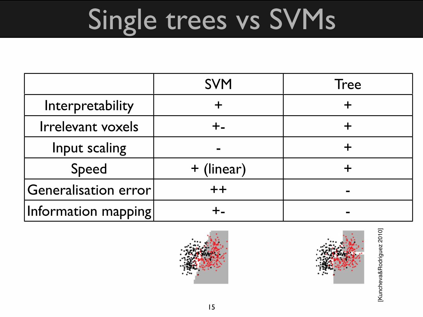
Single trees vs SVMs

15

SVM TreeInterpretability + +

Irrelevant voxels +- +Input scaling - +

Speed + (linear) +Generalisation error ++ -Information mapping +- -

[Kun

chev

a&R

odrig

uez

2010

]

Tutorial agenda

Basics

Growing trees

Ensembling

The random forest

Other forests

Tuning your forests

Information mapping


Datasets

Matlab/PRoNTo

Python/Scikit

Lecture Practical

Single trees tend to have high varianceThe bias-variance tradeoff applies as usual:

We can decrease prediction error arbitrarily on a given dataset, thus yielding low bias.

However, this systematically comes at a price in variance: the parameters of f can change a lot if the training set varies.

Single trees are not ‘stable’ - they tend to reduce bias by increasing variance

17 [Duda et al, 2001]

Ensembling exploits diversityTrain set of classifiers, combine predictions, get reduced ensemble variance and/or bias

Tree diversity has multiple sources

Training set variability/resampling, random projection, choice of cut point (, pruning strategy...)

18

Bagging classifiers generates diversityBagging = Boostrap aggregating

1. Resample with replacement B times from training dataset , yielding

2. Train B base classifiers

3. Get B predictions

4. Combine by majority vote

If the base classifiers have high variance, accuracy tends to improve with bagging since this generates diversity

Good news for trees!

19

S {Sb}, b = 1, . . . , B

{fb}

[Breiman, 1996]

>::sample>>stats::ClassificationBaggedEnsemble >>>sklearn::ensemble

Tutorial agenda

Basics

Growing trees

Ensembling

The random forest

Other forests

Tuning your forests

Information mapping


Datasets

Matlab/PRoNTo

Python/Scikit

Lecture Practical

The random forest bags treesRF combines several diversity-producing methods

1. Generate B bootstrap replicates

2. At each node, randomly select a fewvoxels. Typically or .Since K << D, randomisation is high.

3. No pruning

With a ‘large enough’ number oftrees, RFs typically performs wellwith no tuning on many datasets

21

>adabag::bagging>>stats::TreeBagger, PRoNTo::machine_RT_bin>>>sklearn::RandomForestClassifierRandom projection: [Ho, 1998]

[Kun

chev

a&R

odrig

uez

2010

]

2 4 6 8 10

x 104

50

100

150

200

250

300

number of voxels

ran

do

m p

roje

ctio

n

log2(D)

sqrt(D)

RFs can be seen as probabilistic modelsThe leaf of each tree b can be seen as a posterior (multinomial distribution) pb(y|x)

Ensemble probability:

22

50

100

150

200300

350

400

0

0.5

1

Voxel 2

Voxel 1

More trees = smoother posterior = less over-confidence

RF works for fMRI classification (1)Data: event related fMRI, belief vs disbelief in statements, 14 subjects

Features: ICA timecourse value at button press

23[D

ougl

as e

t al.

2011

]

RF works for multimodal classificationData: 14 HC young, 13 AD old, 14 HC old. Visual stimulation + keypress. fMRI.

Features: fMRI GLM activation-related (n suprathreshold voxels, peak z-score,...), RT, demographics... + feature selection

Classifiers: RF + variants of split criterion. Group classification.

24

[Trip

oliti

et a

l. 20

11]

activation features only + other features

97-99% acc

RF really works for multimodal classificationData: ADNI, 37 AD, 75 MCI, 35 HC. MRI, FDG-PET, CSF measures, 1 SNP

Features: RF as kernel + MDS

25[Gray et al 2013]

Tutorial agenda

Basics

Growing trees

Ensembling

The random forest

Other forests

Tuning your forests

Information mapping


Datasets

Matlab/PRoNTo

Python/Scikit

Lecture Practical

Extremely Randomised Trees increase diversity

Tree variance is due in large part to cutpoint choice. We can generate even more diversity with Extra-trees

Select both K voxels and cutpoints at random, pick best*.

Stop growing when leaves are small

When K=1, called totally randomized trees

+ Accuracy and variance reduction competitive with and sometimes better than RF, faster than RF

27

>extraTrees::extraTrees>>PRoNTo::machine_RT_bin>>>sklearn::ExtraTreesClassifier

Extra-trees: [Geurts et al., 2006]*Dietterich 1998 - the opposite: select top-K best splits, then pick at random

Rotation forests do subspace PCAWe can also generate random rotations of the data to add diversity. For each tree:

1. Project training data X into M random non-overlapping subspaces, each of size K2. For each subspace: choose a subset of classes, draw 75% bootstrap, do PCA

3. Rearrange PCs into a block-diag matrix R and project whole training set to XR.4. Train the tree

28

>Weka via rJava>>Weka via writeARFF or Java>>>?

[Rod

rigue

z et

al.

2006

]

RotFor works for fMRIData: Haxby (8 classes, 90 points per class, 43K voxels)

Tests: feature selection, ensembles vs SVM

29[Kuncheva&Rodriguez 2010]

voxel set size (5-1000)

feat

ure

sele

ctio

n m

etho

d

> SVM (sig)

RF (1000)

> SVM (non-sig)< SVM (sig)

RotFor

Ensemble of FTs may improve accuracyPCA-derived features are multivariate in the original space, so in fact RotFor does axis-parallel (univariate) cuts on MV data...

We can also try slightly more stable MV trees instead of univariate trees (trade diversity for accuracy)

On 62 UCI low-dimensional datasets, it seems that Bagging + FT-leaves works about the same as RotFor + univariate tree* . All other ensembles of univariate trees perform worse...

On high-dimensional fMRI connectivity data**, and low-dimensional graph/vertex attribute representations of fMRI connectivity***, bags of FTs work quite well

30*[Rodriguez et al, 2010] **[Richiardi et al, 2011a] ***[Richiardi et al, 2011b]

Trees ensembles vs SVMs

31

SVM Tree ensemblesInterpretability + +-

Irrelevant voxels +- +Input scaling - +

Speed + (linear) + (parallel)Generalisation error ++ ++Information Mapping +- ++ (see later)

Tutorial agenda

Basics

Growing trees

Ensembling

The random forest

Other forests

Tuning your forests

Information mapping

Correlated features

32

Datasets

Matlab/PRoNTo

Python/Scikit

Lecture Practical

More trees is generally betterFor many tree ensembles, more trees (L) lead to more decrease in variance

Typically use several hundreds to reach plateau (Langs: 40K)

Large L “better approximates infinity” than small L

For RF, the out-of-bag error estimate’s bias decreases a lot with increasing trees - bootstrapping uses ~2/3 of data for each tree, more trees leads to better OOB estimate

This also gives a much smoother posterior distribution

For multivariate trees, use fewer trees

10-30 works well empirically on very different datasets

33

Projection dimension depends on distribution of informativeness

The optimal projection dimension, K, depends on the presence of irrelevant voxels

34

many useful voxels- use small K

info

Gai

n

voxel index

see e.g. [Geurts et al. 2006] for details

information concentratedin few voxels - use large K

info

Gai

n

voxel index

[Diaz-Uriarte et al., 2006]

factor × √D

D=2-10K, N=40-100, C=2-8

Low

-dim

res

ults

Tutorial agenda

Basics

Growing trees

Ensembling

The random forest

Other forests

Tuning your forests

Information mapping

Correlated features

35

Datasets

Matlab/PRoNTo

Python/Scikit

Lecture Practical

Tree ensembles directly provide information maps

The split criterion and related measures are natural indicators of the ‘usefulness’ of voxels in the discrimination task

But they are unsigned

They are computed at each node of the tree, so we can aggregate them over trees to get stable estimates

Different ensembles provide different information maps, and we can use other data than split criteria to map

36

Information mapping: RF/Gini importance

GI of a voxel: infoGain (compute with Gini impurity) for this voxel, averaged over all trees in ensemble

37[Langs et al., 2011]

Information mapping: RF/GI/var

38

0 500 1000 1500

0.05

0.1

0.15

0.2

voxel index

Gin

i im

po

rta

nce

Information Mapping: L2 SVM

39

0 1 2 3 4 5 6

x 104

!0.6

!0.4

!0.2

0

0.2

0.4

0.6

0.8

1

voxel index

Weig

ht in

prim

al

Information mapping - Regional GI

40[Gray et al 2013]

Data: ADNI, 37 AD, 75 MCI, 35 HC. MRI, FDG-PET, CSF measures, 1 SNP

sMRI

PET

Information mapping: RF/Variable importance

VI of a voxel*: average loss of accuracy on OOB samples when randomly permuting values of the voxel

This is suboptimal with correlated voxels

Permuting one single variable ignores correlations

With several relevant & correlated voxels, they could be deweighted because removing one does not deteriorate accuracy

VI is well-correlated with GI**

More on this later

41*[Breiman, 2001] **[Strobl et al., 2007]

Information mapping: bag of FTsLeaves in an FT can be regression models

These can be trained using any method, in practice LogitBoost (iterative reweighting) works wellThe importance of a voxel is its average regression weights across trees and folds

42

−60 −40 −20 0 20 40 60−100

−80

−60

−40

−20

0

20

40

60

TempMidR

TempPoleR

CunR

left−right

CunLOccInfL

posterior−anterior

−100 −80 −60 −40 −20 0 20 40 60−40

−20

0

20

40

60

TempPoleR

posterior−anterior

TempMidROccInfL

CunRCunL

ventral−dorsal

[Richiardi et al. 2011a]

Information mapping from accuracyFinally we could also map results directly from classifier with best accuracy

Here: Haxby data, SVM-RFE 200, RF1000, intersection of selected features across 10 folds, one slice

43[Kuncheva et al. 2010]

Tutorial agenda

Basics

Growing trees

Ensembling

The random forest

Other forests

Tuning your forests

Information mapping

Correlated features

44

Datasets

Matlab/PRoNTo

Python/Scikit

Lecture Practical

Correlated features are picked up by tree ensembles

With regularisers in SVMs, correlated features will be deweighted (L2) or left out (L1)

Tree ensembles have grouping effect*, where correlated but informative features can survive with high weight

Empirically this seems to depend on tree depth... 45*[Langs et al., 2011]

[Per

eira

& B

otvi

nick

, 201

1]

There are ways of dealing with correlated features

Several proposals from bioinformatics have attempted to tackle the GI/VI measure bias

Conditional Variable Importance only permutes a correlated variable within observations where its correlands have a certain value (accounts for correlation structure)

Permutation IMPortance fixes for under-importance of grouped vars by permuting class labels, then constructing a null distribution of GI values

These methods can be used in neuroimaging directly...

46Cond. Var. Imp. [Strobl et al, 2008]

PIMP [Altmann et al., 2010] >party::cforest

Tutorial agenda

Basics

Growing trees

Ensembling

The random forest

Other forests

Tuning your forests

Information mapping


Datasets

Matlab/PRoNTo

Python/Scikit

Lecture Practical

Datasets1. SINGLE SUBJECT: SPM Auditory - “Mother of All Experiments” - 1 subject, 2T scanner, TR=7s, 6 blocks of 42 s rest, 42s auditory stimulation. Task: two-class intra-subject decoding: auditory vs rest.

2. GROUP COMPARISON: Buckner checkerboard - 41 subjects from three groups, young (18-24), elderly healthy (66-89) and elderly demented (age 68-83). Four runs per subject, 128 volumes per run with TR=2.68s.Task: classify young (n=28) versus old (n=30) group based on ‘first level’ beta maps

49Original auditory data at www.fil.ion.ucl.ac.uk/spm/data/auditory/ Original visual data at fmridc.org

[Buckner et al., 2001]

http://www.fil.ion.ucl.ac.uk/spm/data/auditory/






Tutorial agenda

Basics

Growing trees

Ensembling

The random forest

Other forests

Tuning your forests

Information mapping


Datasets

Matlab/PRoNTo

Python/Scikit

Lecture Practical

The PRoNTo toolboxMatlab code, open source, GUI / batch / scripting

Users can quickly test machine learning methods without coding

51

http://www.mlnl.cs.ucl.ac.uk/pronto/



Start PRoNTo1. Make sure your path is setup properly

>> which spm>> which pronto

2. Start PRoNTo

>> pronto

52

Tutorial agenda

Basics

Growing trees

Ensembling

The random forest

Other forests

Tuning your forests

Information mapping


Datasets

Matlab/PRoNTo

Python/Scikit

Lecture Practical

Scikit-learn / niPyA very good alternative for python fans is to use Scikit-learn + niPy. It has RF, Extra-trees, and others

For people that missed Gaël’s tutorial at PRNI 2011: http://nisl.github.io/

PyMVPA also has access to Extra-trees and RF

54

http://nisl.github.io

http://nisl.github.io

ConclusionsTree ensembles can offer competitive decoding performance with SVMs, and are good for multimodal classification

They produce information maps which are typically sparser than L2 SVMs (is this good or bad?), and can have different interpretation

Implementations abound in the language of your choice, including R, Matlab, Python

So... take a walk in the forest for your next project

55

ThanksFINDlab, Stanford University

A. AltmannComputational Image Analysis and Radiology, Medical U. of Vienna / CSAIL, MIT

G. LangsMontefiore Institute, U. of Liège

P. GeurtsFIL, UCL

G. ReesPRoNTo team members @ UCL, KCL, U. Liège, NIH

J. Ashburner, C. Chu, A. Marquand, J. Mourao-Miranda, C. Phillips, J. Rondina, M. J. Rosa, J. Schrouff + João de Matos Monteiro

Computer Vision Group, U. FreiburgA. Abdulkadir

56

Modelling and Inference on Brain networks for Diagnosis, MC IOF #299500

Useful references - booksCriminisi, A. and Shotton, J. (eds) (2013). Decision forests for computer vision and medical image analysis, Springer

Hastie et al. (2011). The Elements of Statistical Learning, Springer.

MacKay, D.J.C. (2003). Information Theory, Inference, and Learning Algorithms, Cambridge University Press

57

References in tutorialAltmann, A. et al. (2010). Permutation importance: a corrected feature importance measureBreiman, L. (1996). Bagging Predictors, Machine Learning 24Diaz-Uriarte et al. (2006). Gene selection and classification of microarray data using random forest. BMC Bioinformatics 7:3Douglas, P.K. et al. (2011). Performance comparison of machine learning algorithms and number of independent components used in fMRI decoding of belief vs. disbelief. NeuroImage 56.Gama, J. (2004). Functional Trees. Machine Learning 55Geurts P. et al. (2006). Extremely randomized trees, Machine Learning 63:3-42Gray, K. et al. (2013). Random forest-based similarity measures for multi-modal classification ofAlzheimer's disease. NeuroImage 65.Ho, T. K. (1998). The random subspace method for constructing decision forests. IEEE TPAMI 20(8)Kuncheva, L.I. and Rodriguez, J.J. (2010). Classifier ensembles for fMRI data analysis: an experiment. Magnetic Resonance Imaging 28Langs, G. et al. (2011). Detecting stable distributed patterns of brain activation using Gini contrast. NeuroImage 56(2)Mourao-Miranda, J. et al. (2005). Classifying brain states and determining the discriminating activation patterns: Support Vector Machine on functional MRI data. NeuroImage 28.Pereira, F., Botvinick, M. (2011). Information mapping with pattern classifiers: A comparative study. NeuroImage 56(2).Rodriguez, J.J. et al. (2006). Rotation Forest: A New Classifier Ensemble Method, IEEE TPAMI 28(10)Rodriguez, J.J. et al. (2010). An Experimental Study on Ensembles of Functional Trees. Proc. MCSStrobl, C. et al. (2008). Conditional variable importance for random forests. BMC Bioinf. 9:307Tripoliti, E. E. et al. (2011). A supervised method to assist the diagnosis and monitor progression of Alzheimer’s disease using data from an fMRI experiment. Artificial Intelligence in Medicine 53

58

More referencesRichiardi, J. (2007). Probabilistic models for multi-classifier biometric authentication using quality measures. Ph.D. thesis, EPFL.Richiardi, J. et al. (2011a). Decoding brain states from fMRI connectivity graphs. NeuroImage 56Richiardi, J. et al. (2011b). Classifying connectivity graphs using graph and vertex attributes. Proc. PRNI

59

alternatives to support vector machines in...

Documents