Am I my peer’s keeper? Social Responsibility in Financial Decision Making

Sascha Füllbrunn and Wolfgang J. Luhan

Creating knowledge for society

Nijmegen, April 2015NiCE15-03

Working paper

Am I my peer's keeper? Social Responsibility in

Financial Decision Making

Sascha Füllbrunn∗, and Wolfgang J. Luhan†‡

April 7, 2015

Abstract

Decision makers often take risky decisions on the behalf of others

rather than for themselves. Competing theoretical models predict both,

higher as well as lower levels of risk aversion when taking risk for others,

and the experimental evidence is mixed. In our within-subject design,

money managers have substantial responsibility by taking investment de-

cisions for themselves and for a group of six clients, when payments are

either �xed or perfectly aligned. We �nd that money managers invest

signi�cantly less for others than for themselves (cautious shift) which is

mainly driven by a less risk averse sub sample. Digging deeper we �nd

money managers to rather act in line with what they believe the clients

would invest for themselves. We derive a responsibility weighting func-

tion to show that with a perfectly aligned payment the money manager

weights egoistic and social preferences. Finally we bring our results in

perspective with the mixed experimental literature.

JEL: C91, D81, G11

Keywords: �nancial decision making, social responsibility, decision making for others, risk

preferences, experiment

∗Radboud University, Institute for Management Research, Department of Economics,Thomas van Aquinostraat 5, 6525 GD Nijmegen, The Netherlands (s.fullbrunn@fm.ru.nl)†Institute for Macroeconomics & Bochum Lab for Experimental Economics (RUBεχ),

Ruhr-University Bochum, Universitaetsstrasse 150, 44801 Bochum, Germany (wolf-gang.luhan@rub.de)‡We gratefully acknowledged funding by the Ruhr-University Bochum's Young Researchers

Funds.

1

1 Introduction

The vast majority of economic decisions involve certain levels of uncertainty

about the outcome. Economic research on risk attitudes has traditionally fo-

cused on individual decision making issues, without any consideration for po-

tential social in�uences on risk preferences (see e.g., Dohmen et al., 2011; Eckel

and Grossman, 2008b; Harbaugh et al., 2010; Holt and Laury, 2002). As real

world decisions are embedded in a social context, however, a decision makers is

hardly ever the only person a�ected by the consequences of his actions. Indeed,

many risky decisions do not only a�ect but are speci�cally taken on behalf of a

third party. This third party might be the decision maker's family or a business

partner; on a larger scale CEO's decisions a�ect a company or even an industry,

and political decisions a�ect large parts of the population, a nation or beyond.

On �nancial markets, investors usually put an agent in charge of his risky in-

vestments. During the �nancial crisis of 2007-2008 this practice in the �nancial

sector became the subject of a continuing public as well as a scienti�c debate as

it was perceived to lead to excessive risk taking (Allen and Gorton, 1993; Allen

and Gale, 2000; Cheung and Coleman, 2014; Kleinlercher et al., 2014; Robin

et al., 2011). Though responsibility in risky decisions has only recently been

picked up in the experimental literature (see Trautmann and Vieider (2012) for

a review and section 2). The results, however, provide no consistent answer

concerning the question of whether decisions on behalf of others involve higher

(risky shift) or lower (cautious shift) levels of risk as compared to decision for

oneself.

The terms �risky shift� and �cautious shift� were introduced by Stoner (1961)

to describe situations where the initial, individual level of risk preference is al-

tered due to exogenous impacts. In the case of responsibility the resulting shift

could be in both directions. In the psychological literature, a prominent explana-

tion for a risky shift is the �psychological self-other distance� (e.g., Beisswanger

et al., 2003; Cvetkovich, 1972; Stone and Allgaier, 2008; Trope and Liberman,

2010; Wray and Stone, 2005) in which the evaluation of a potential loss in a

risky situation is decreasing in the distance to the decision maker. This �nd-

ing translates directly to the results from economic experiments (e.g., Harrison,

2006; Holt and Laury, 2002, 2005), as risk aversion is signi�cantly decreased in

hypothetical situations without real consequences in the laboratory1. Further

support for this �nding comes from neuro-economics. Albrecht et al. (2011)

�nd that making inter-temporal decisions for others result in lesser activation of

areas of the brain that are thought to be engaged in emotion and reward-related

1Noussair et al. (2014) �nd barely a di�erence between hypothetical and incentivized riskelicitation techniques using lotteries. Though in their study they considered the di�erencewithin the online subject pool, but not in the laboratory.

2

processes than when taking decisions for oneself.

The resulting argument would be that decisions made on behalf of a third

party are equivalent to situations without any real outcome. In contrast, Char-

ness and Jackson (2009) propose �responsibility alleviation� (Charness, 2000)

as an explanation for a cautious shift. According to this theory, taking respon-

sibility for a third party's welfare induces pro-social behavior which results in

conservative risk taking (Charness, 2000; Charness and Jackson, 2009). Though

pro-social behavior can also mean that the decision maker tries to match the

will of the others.

Despite prominent examples of a risky shift in �nancial markets due to lim-

ited liability of money managers (e.g., Allen and Gorton, 1993), there are several

empirical observations on cautious shift behavior. Physicians, for example, have

been found to prefer treatments with higher mortality rates for themselves than

what they recommend to their patients (Garcia-Retamero and Galesic, 2012;

Ubel et al., 2011). Managers try to avoid responsibility for decisions with even

a minimal probability of hazardous outcomes (Swalm, 1966; Viscusi et al., 1987).

We study the e�ect of responsible �nancial decision making for others using

a series of economic laboratory experiments. We �rst discuss design features

from previous studies that might have triggered certain directions of investment

shifts, i.e. increased risk taking for others (risky shift) or decreased risk taking

for others (cautious shift). We then implement an experimental design that

controls for these potential confound e�ects. In contrast to the literature, we

consider a design with high responsibility (six clients) in a situation with and

without payo� alignment of the decision maker. We discuss several behavioral

theories that might explain the con�icting results in the literature.

In our experiment, an individual decision maker (henceforth �the money

manager�) faces a risky investment situation similar to Gneezy and Potters

(1997). In our three treatments the money manager either invests only for

himself, only for a group of six other subjects (henceforth �the clients�) without

any monetary relevance for himself (no payo� alignment), or he invests an equal

amount for the clients and for himself (payo� alignment). This enables us to

systematically study the e�ect of social responsibility on risk aversion as well as

the e�ect of possible di�erences between the money manager's and his clients'

risk preferences. We found the existing literature to equalize two profoundly

di�erent situations, one in which the money manager's payo� is perfectly aligned

with the clients' payo�, i.e., the money managers take the same risk, and one

in which the money manager's payo� is independent of his investments. Our

study is the �rst to systematically compare these theoretically very di�erent

situations and to attempt to identify a unifying behavioral explanation for the

mixed results in the literature.

3

Our aggregate results indicate investment behavior to be in line with respon-

sibility alleviation as the money managers invest signi�cantly less when clients

bear the consequences even when the money manager's payo� depends on his

investment. However, this cautious shift is purely driven by money managers

with low levels of risk aversion. For money managers with high levels of risk

aversions, we �nd indications for a risky shift. Apparently, when making de-

cisions for others the money managers try to act according to the clients' risk

preferences. Eliciting the money manager's beliefs about the clients' propensity

to invest from themselves, we indeed �nd that money managers on average in-

vest an equal amount for their clients they believe the clients would invest for

themselves. In the case of payo� alignment, we �nd that the di�erence between

his own risk preference and the perceived risk preferences of the group deter-

mines the decision. We �t a weighted preference function to our data allowing

us to determine the level of altruism of our subjects. On average the money

managers display a signi�cant amount of responsibility. However, they assess

their individual preferences to be more important than those of the six clients.

2 Literature Review

There is a small, yet growing body of literature on risky decision making for

others with rather mixed results (�nd an overview in table G.10 in the online

supplement). A number of studies �nd evidence for a risky shift, i.e. money man-

agers take a signi�cantly higher risk for others than for themselves. Chakravarty

et al. (2011) �nd that subjects tend to be less risk averse when deciding for oth-

ers, using a �rst price sealed bid auction against computer bidders as well as

a multiple price list. They conclude that decision makers display social prefer-

ences when deciding for others but also argue, though do not test, that decision

making for others is not di�erent from hypothetical risk taking. Results from

a multiple price list design in Andersson et al. (forthcoming), though insigni�-

cant, suggest rather a risky shift. Using structural estimation they argue that

loss aversion is reduced when investing for others. Polman (2012) �nds a risky

shift when considering a multiple price list in his third study.2 Using the Gneezy

and Potters (1997) investment game with repetition, Pollmann et al. (2014) and

Sutter (2009) �nd a signi�cant risky shift. 3

In contrast, a cautious shift, i.e., money managers take signi�cantly lower

2One needs to be careful when interpreting the results in Polman (2012).The incentives forthe decision maker are not salient and a part of the reported experiments involve deception.

3In PAY-COMM, a team consisted of three members. One member needed to make adecision for the �rst three periods, a second member for the second three periods, and the lastmember for the last three periods. While the �rst member showed no shift at all, the secondand the third showed a signi�cant risky shift.

4

risks for the clients than for themselves, has been found by an even larger number

of studies. In Reynolds et al. (2009) the money manager decides between a safe

and a risky choice for himself �rst, and subsequently for each individual in a

group of clients (three to �ve subjects). They �nd the number of safe choices

to be in general higher for others than for the money manager himself. Eriksen

and Kvaløy (2010) replicate the experiment from Gneezy and Potters (1997) but

added a treatment in which money managers invest the endowment of one client

only. Investments are signi�cantly lower when investing for clients than when

investing for the money manager himself. As a control they reran the treatment

with hypothetical clients and found investment levels to be signi�cantly higher.4

Montinari and Rancan (2013) used a similar version to Eriksen and Kvaløy

(2010) but with lotteries yielding a negative expected return. Still the money

managers invested more for themselves than for their clients, especially if the

client was a friend of the money manager. Charness and Jackson (2009) consider

strategical risk taking in the stag-hunt game in which two players choose either

stag (risky) or hare (risk-less). They report lower numbers of stag-plays when

the payo� consequences are shared with another subject, concluding that their

result is in line with a responsibility alleviation e�ect (Charness, 2000). In the

�rst setting of Bolton and Ockenfels (2010) subjects choose between a risky

choice and a safe choice for oneself and others or only for others. They �nd

a cautious shift with the number of safe choices being lower for others than

for oneself only. They suggest a tendency to take conservative risk when one's

choice a�ects other people's welfare. Bolton et al. (2015) �nd further evidence

in line with this suggestion using a multiple price list design.

Using a battery of lotteries and similar decisions for oneself and a third party,

Pahlke et al. (2012) provide evidence for a risky shift in the loss domain and a

cautious shift in the gain domain for moderate probabilities; and a reversal for

small probabilities. They conclude that their results �discredits hypotheses of a

'cautious shift' under responsibility, and indicates an accentuation of the fourfold

pattern of risk attitudes usually found for individual choices� (p.22). Finally

Humphrey and Renner (2011) using a multiple price list �nd no signi�cant shift

at all.

Thus, the evidence is as mixed as are the experimental designs. Although

describing a (largely) similar situation, the studies mentioned di�er in various

aspects. With the oppositional �ndings of a risky as well as a cautious shift,

the obvious conclusion is that the di�erences in design might be driving the

di�ering results. Our approach is therefore to identify confounding factors and

4The result in Eriksen and Kvaløy (2010) is further evidence for the e�ects of self-otherdistance in risky decisions (e.g., Beisswanger et al., 2003; Cvetkovich, 1972; Stone and Allgaier,2008; Trope and Liberman, 2010; Wray and Stone, 2005). More importantly it indicates thatthis will produce results similar to hypothetical decision making (e.g., Harrison, 2006).

5

systematically exclude or control them in our experimental design.

The �Others�. All studies listed above consider �risk taking for others� and

focus on the di�erence between making a decision for oneself (henceforth OWN)

and making the same decision for a client. There is, however, an important vari-

ation in the payo� alignment between money managers and clients. Either the

money manager decides for the clients only and earns a lump sum payment

(henceforth OTH - decision for clients only)5, or the money manager has to

invest the same amount as the clients, i.e., money manager and clients take the

same risks (henceforth LEA - same decision for oneself and clients).6 Although

these situations are obviously not similar, as the own consequences di�er� the

previous literature has exclusively considered either OTH or LEA when consid-

ering decision making for others.7 Standard models of rational behavior make

clear predictions on risk taking in LEA. In this case, egoistic preferences play

the main role and investments in OWN are not distinguishable from investments

in LEA.8 In OTH there is no standard-theoretical prediction as the decision for

others has no monetary impact in for money manager's payo� (Eriksen and

Kvaløy, 2010). We implement both treatments along with the decision for one-

self in a within-subjects design, to examine whether money managers in LEA

invest in a rather sel�sh manner (LEA=OWN) or rather in line with what they

would for the others only (LEA=OTH).

Responsibility. Apart from Sutter (2009)9 the previous studies consider de-

cision making for one client only. We expand the responsibility for the money

manager as each has to manage a 54-Euro-fund for six clients. According to

responsibility alleviation (Charness, 2000; Charness and Jackson, 2009) the ef-

fects of responsibility should be increasing in the number of a�ected parties.

Therefore, any e�ects observed in previous studies, should be ampli�ed in our

setting.

Accountability. Accountability, i.e., the fact that the money managers can

be blamed for their decision, has been shown to be an important factor when

making risky decisions for others. Pollmann et al. (2014) provide evidence for

a reduction in risk taking for others under accountability. This might also

hold true for implicit accountability in the sense that the clients are able to

5Studies comparing OWN with OTH are Eriksen and Kvaløy (2010); Chakravarty et al.(2011); Reynolds et al. (2009); Polman (2012); Andersson et al. (forthcoming); Montinari andRancan (2013); Pollmann et al. (2014). See tableG.10 in the online supplement.

6Studies comparing OWN with LEA are Charness and Jackson (2009); Sutter (2009);Bolton and Ockenfels (2010); Humphrey and Renner (2011); Pahlke et al. (2012); Anderssonet al. (forthcoming); Bolton et al. (2015), see tableG.10 in the online supplement.

7 Andersson et al. (forthcoming) conduct experiments on both OTH and LEA but do notdiscuss theoretical consequences nor do they compare the observed di�erences between OTHand LEA.

8 Note that ex ante or ex post fairness plays no role as the money manager and the clientreceive the same payo�.

9A LEA setting in which the money manager has to decide for a group of three.

6

observe the money manager's decision albeit they do not know the identity of

the money manager (Eriksen and Kvaløy, 2010). In this light, accountability

could have a�ected the results of Reynolds et al. (2009) as the decision was

openly announced to the group. Obviously, this holds as well in decisions made

for a friend (Humphrey and Renner, 2011; Montinari and Rancan, 2013). To

rule out accountability as a confounding e�ect, our clients are not able to infer

the identity of a money manager nor are they able to observe the decision during

the decision making process.

Repetition. Sutter (2009) as well as Eriksen and Kvaløy (2010) consider

the Gneezy and Potters (1997) investment game with repetition. Here, money

managers were not only able to experience the game. They are also able to

accumulate wealth and may thus adjust their behavior according to gains or

losses in earlier rounds.. Interestingly, the �rst study (LEA) �nds a risky shift

and the second (OTH) �nds a cautious shift. One reason might be the di�erence

in the design. While in Eriksen and Kvaløy (2010) one money manager decides

in all periods, in Sutter (2009) group members took turns in making decisions

for the group every three periods. Implicit accountability might explain these

di�erences as the clients were able to observe the decisions of the money man-

ager. However, in our design the clients have to bear consequences of only one

decision by the money manager, i.e., money managers were not able to diversify

across periods.

Anchoring. In Reynolds et al. (2009), the money manager �rst made a

decision for himself, observed the results of his investment, and then made a

decision for the others. The feedback for the �rst decision, however, alters

the information set for the subsequent decision. This situation could trigger

psychological anchoring e�ects such as gamblers fallacy or hot hand belief (see

e.g., Huber et al., 2010). In Sutter (2009), each decision taken was observed by

the whole group, so even if the decision maker took his �rst turn, his decisions

were in�uenced by the observations of previous outcomes. This procedure might

explain the observation of decreasing risk aversion over the nine subsequent

decisions. In our design, the participants receive information on the outcome

of their investment only at the end of the experiment, thereby keeping the

information set in all decisions constant.

Order e�ects. Most of the studies consider a between-subjects design. But

Montinari and Rancan (2013) consider a within-subject design replicating Erik-

sen and Kvaløy (2010), though with a negative expected period return. The

sequence of action was as follows. Money managers �rst invested twelve times

for themselves (OWN), followed by twelve investments for others (OTH), and

twelve investments for friends (OTH). Thus, learning over 36 repetitions alone

might lead to a reduction in risk taking. However, Montinari and Rancan (2013)

7

conclude to observe a cautious shift comparing the treatments. Unfortunately,

they cannot rule out experience as a confound e�ect as they did not control for

order e�ects. We consider a within-subject design as well, but control for order

e�ects by implementing an AB/BA design.

Self-other distance. A further argument for di�erent results might be ex-

plained by self-other distance. Among others, Eriksen and Kvaløy (2010) show

that investments for hypothetical clients lead to signi�cantly higher risk taking

than for real clients in the laboratory. However, Andersson et al. (forthcoming)

�nd no signi�cant di�erences when comparing a hypothetical risky decision and

a risky decision with an e�ect for others in an internet experiment with higher

social distance. These results indicate that laboratory experiments seem to in-

crease the perception of making decisions for real clients (closer social distance)

not for a potentially hypothetical ones in the internet (higher social distance).

Fairness. Finally, one might argue that fairness preferences play a role when

payments for the money managers are �xed or known beforehand in OTH as for

example in Eriksen and Kvaløy (2010), Reynolds et al. (2009) or Chakravarty

et al. (2011). A money manager receiving a small �xed payo� might make

smaller investments for his clients if he perceives that high investments might

create payo� inequalities to his disadvantage. Reversely, a high �xed payo�

might induce a money manager to make high investments for his clients. To

control for this issue, we varied the �xed payo� for the money manager when

investing for his clients (OTH). In one setting, the money manager earns the low-

est and in a second setting the highest possible payo� the clients could achieve.

To sum up, we design a situation in which a money manager makes a risky

investment for six clients. His payo� is either perfectly aligned with the clients'

payo�s (LEA) or not aligned at all (OTH). We do not consider incentive com-

patible contracting in a principal-agent relationship, but focus on the pure e�ect

of responsibility for a third party. We control for fairness issues, concerning the

allocation of resources (Fehr and Schmidt, 1999; Bolton and Ockenfels, 2000;

Charness and Rabin, 2002, 2005), and ex ante and ex post fairness consider-

ations (see Fudenberg and Levine, 2012), exclude accountability, and test for

order e�ects. Finally, we do not consider competition among money managers

as in Agranov et al. (2014) but focus purely on changes in risk taking when

making investment decisions for others.

8

3 Design and Procedure

3.1 Treatments

We consider the Gneezy and Potters (1997) investment setting as the �relative

simplicity of the method, combined with the fact that it can be implemented

with one trial and basic experimental tools, makes it a useful instrument for

assessing risk preferences� (Charness et al., 2013, p. 45).10 In our baseline

treatment (OWN), each subject is endowed with 9 Euro and is asked to decide

on the amount to invest in a risky asset. With a probability of 2/3 the amount

invested is lost and with a probability of 1/3 the investment earns a return of

250 percent. For X ∈ {0, 9} being the amount invested, the payo� was either

πOWN = 9−X, in case of a loss, or πOWN = 9 + 2.5X, in case of a win.

In treatment OTH, subjects are organized in groups of seven, consisting

of six passive members, the clients (c), and one active member, the money

manager (m). Each client, is endowed with 9 Euro and the money manager

decides on the amount to invest in the risky asset for each of the six clients.

The amount invested is identical for all clients. The payo� for each client is

either πOTHc = 9 − X, in case of a loss, or πOTHc = 9 + 2.5X, in case of a

win. The payo� for the money manager in any case is πOTHm = 0, which is

common knowledge. To control for possible e�ects due to fairness preferences

(see section 2) we also implement a treatment in which the money managers

payo� was πOTHc = 31.5, which is, again, common knowledge.

In treatment LEA, we implement the same group protocol as in OTH. In

contrast to OTH, all subjects including the money manager, are endowed with

9 Euro. The money manager decides on the amount to invest for each of the six

clients and for himself. The amount invested is identical for all group members.

The payo� is either πLEAc = πLEAm = 9−X, in case of a loss, and πLEAc = πLEAm =

9+2.5X, in case of a win, for all group members including the money manager.

3.2 Implementation

The experiment was conducted at the Ruhr-University Bochum experimental

laboratory (RUBεχ). The experiment was programmed and conducted with

the software z-Tree (Fischbacher, 2007). We administered a within-subject de-

sign as subjects made their decision in each of the three treatments. Upon ar-

rival subjects were randomly placed at computer terminals separated by blinds.

10Note that risk-neutral (and, in turn, risk-seeking) individuals should invest their entireendowment. Hence, this method cannot distinguish between risk-seeking and risk-neutralpreferences. Though usually only a fairly small fraction of participants choose to invest theentire amount. The amount invested provides a good metric for capturing treatment e�ectsand di�erences in attitude toward risk between individuals. See Charness et al. (2013) for adetailed discussion.

9

In each treatment, instructions were read aloud and questions were answered

privately. The experiment only started once we were sure all participants had

comprehended the instructions. Once the treatments started, subjects were en-

dowed with an on-screen calculator where they could enter arbitrary investment

levels. The calculator would display a list containing all entered investment

levels, the respective own payo� and (in case of OTH and LEA) the clients

payo� in case of a loss and in case of a win.11 Subjects subsequently chose one

investment level from the generated list and con�rmed their choice. To exclude

repetition e�ects, participants were only informed that the experiment would

consist of three independent parts, without specifying the exact nature of each

part upfront. The instructions for each part were distributed only after the

previous part was concluded. Subjects did not receive any feedback on their

decisions until the end of the experiment.12 After the last treatment, subjects

had to answer a short debrie�ng questionnaire.

In the OTH and LEA treatments, each subject �rst made an anonymous

investment decision in the role of a money manager for each of the six clients in

the group (OTH) or for the whole group including himself (LEA). But at the end

of the experiment, the investment decision of only one randomly drawn money

manager in a group was binding for all group members. This procedure was

common information. To avoid accountability e�ects, we guaranteed anonymity.

Neither the money managers knew the identity of the clients nor did the clients

know the identity of the money manager. We informed the subjects that only

one of three treatments is payo� relevant. At the end of a session, we threw a

dice to determine the payo� relevant treatment and we threw a dice for each

group to determine whether the investment was successful or not. Subjects were

payed privately and in cash and left the lab.

We ran 15 sessions with a total of 175 participants. Our participants were

mostly bachelor students from all departments of the Ruhr-University Bochum.

Subject participated only once in this experiment. We implemented three di�er-

ent setups. In setup one (70 observations), the treatment order was OTH-OWN-

LEA. In setup two (70 observations), the treatment order was LEA-OWN-OTH.

In setup three (35 observations), we reran setup one but the money manager

earned the highest possible amount, i.e., πOTHm = 9+2.5×9 = 31.50 Euro (which

was also common knowledge). Comparing setup one to setup two we �nd no

order e�ect and comparing setup one to setup three we �nd no e�ect on the

payment condition.13 Thus, we pool the data and end up with 175 independent

observations. For those who are interested in gender e�ects, we provide a short

11A short description on how subjects decided including a screenshot can be found in theonline supplement section E.12Find instructions in the online supplement in section F.13We provide test results in the online supplement section A.

10

analysis in the online supplement showing that decisions do not signi�cantly dif-

fer comparing male and female money managers. Average payments were 15.60

Euro (max. 34.5, min. 3) including a show-up fee of 3 Euro for the duration of

roughly half an hour.

3.3 Hypotheses

We are not interested in individual investments for oneself (OWN) but rather

in the shift of investments comparing OWN and OTH, and OWN and LEA

respectively. Standard models of perfectly rational, egoistic agents make no

predictions about situations like OTH as the payment for the money manager is

not aligned to the investment decision (e.g., Eriksen and Kvaløy, 2010). Eriksen

and Kvaløy (2010) as well as Andersson et al. (forthcoming) pick up the self-other

distance hypothesis arguing that loss aversion is less pronounced when deciding

for others than when deciding for oneself in line with the self-other distance,

i.e., XOWN < XOTH. The social responsibility hypothesis, however, argues that

money managers behavior - driven by responsibility alleviation (Charness, 2000;

Charness and Jackson, 2009) - will be more conservative when investing for oth-

ers, i.e., XOWN > XOTH. When the money manager believes his clients to have

similar risk preferences as himself, he would, in line with the false consensus

e�ect (Ross et al., 1977), invest the same amount for himself and for the clients,

i.e., XOWN = XOTH. In contrast, the self-others discrepancy e�ect states that

money managers evaluate their own risk preferences di�erently than the risk

preferences of their clients (Hsee and Weber, 1997; Eckel and Grossman, 2008a;

Leuermann and Roth, 2012). Thus, the predicted shift depends on the risk atti-

tudes of the money managers relative to their clients. If money managers believe

the clients to be relatively risk averse, they would invest less for the clients then

for themselves (XOWN > XOTH), while money managers who believe the clients

to be relatively risk seeking, would invest more for the clients then for them-

selves (XOWN < XOTH). This could be one possible explanation for the mixed

results in the literature. Studies �nding a risky shift might simply feature a

rather risk averse sample of the population, as studies reporting a cautious shift

might by chance have a sample of rather risk loving money managers. To our

knowledge, this has not been examined in the previous literature so far.

In contrast to OTH, rational models make clear predictions on risk taking in

LEA. Excluding other-regarding preferences, decisions in OWN and LEA should

not di�er, i.e., XOWN = XLEA. However, when the money manager's payo� is

perfectly aligned with the clients' payo�s, egoistic preferences will be opposed

by any social preference theory following the same predictions as for OTH.

Thus, when the social preferences for clients completely crowd out the egoistic

11

preferences of the money manager there is no di�erence to the situation without

payo� alignment, i.e., XLEA = XOTH. When both preferences play a role, we

hypothesize the investments in LEA to be in-between investments in OWN and

OTH, i.e., either XOWN ≥ XLEA ≥ XOTH or XOWN ≤ XLEA ≤ XOTH. Note

that the interaction of social and/or egoistic preferences in risky decision making

can only be studied when all three treatments are considered in a within-subjects

design.

4 Results

4.1 Risky or Cautious Shift?

Do the data show a risky shift or a cautious shift when making risky decisions

for others? To answer this question, we compare each subjects investment in

LEA (XLEAi ) and OTH (XOTH

i ) to the investment in OWN (XOWNi ) by cal-

culating the shift in investments, i.e., SLEAi = XLEAi − XOWN

i and SOTHi =

XOTHi −XOWN

i , as the relevant unit of observation. Note that negative values

indicate a cautious shift and positive values indicate a risky shift. The second

column in table 1 provides averages of investments and shifts for 175 indepen-

dent observations.

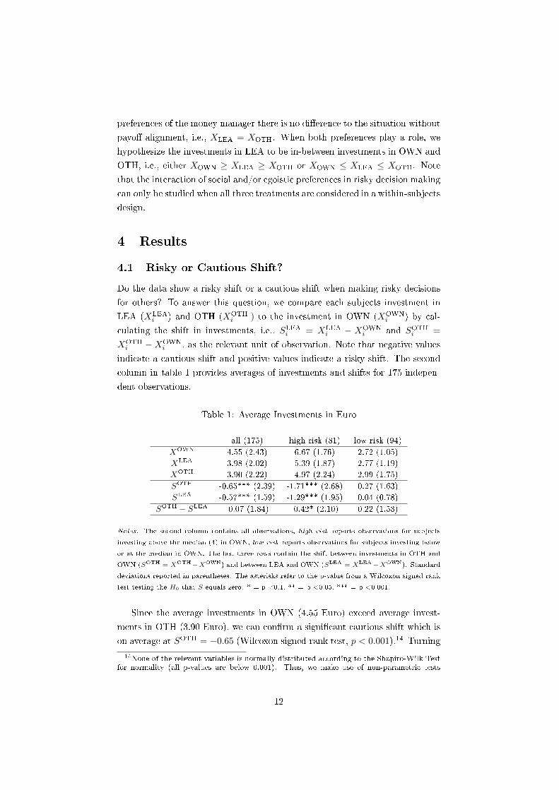
Table 1: Average Investments in Euro

all (175) high risk (81) low risk (94)

XOWN 4.55 (2.43) 6.67 (1.76) 2.72 (1.05)

XLEA 3.98 (2.02) 5.39 (1.87) 2.77 (1.19)

XOTH 3.90 (2.22) 4.97 (2.24) 2.99 (1.75)

SOTH -0.65*** (2.39) -1.71*** (2.68) 0.27 (1.63)

SLEA -0.57*** (1.59) -1.29*** (1.95) 0.04 (0.78)

SOTH − SLEA -0.07 (1.84) -0.42* (2.10) 0.22 (1.53)

Notes. The second column contains all observations, high risk reports observations for subjects

investing above the median (4) in OWN, low risk reports observations for subjects investing below

or at the median in OWN. The last three rows contain the shift between investments in OTH and

OWN (SOTH = XOTH−XOWN) and between LEA and OWN (SLEA = XLEA−XOWN). Standard

deviations reported in parentheses. The asterisks refer to the p-value from a Wilcoxon signed rank

test testing the H0 that S equals zero. * = p <0.1, ** = p <0.05, *** = p <0.001.

Since the average investments in OWN (4.55 Euro) exceed average invest-

ments in OTH (3.90 Euro), we can con�rm a signi�cant cautious shift which is

on average at SOTH = −0.65 (Wilcoxon signed-rank test, p < 0.001).14 Turning

14None of the relevant variables is normally distributed according to the Shapiro-Wilk Testfor normality (all p-values are below 0.001). Thus, we make use of non-parametric tests

12

to a situation in which egoistic preferences may play a role, we again con�rm

a signi�cant cautious shift which is on average at SLEA = −0.57 (Wilcoxon

signed-rank test, p < 0.001) as in LEA the average investment drops to 3.98

Euro. Thus, we state observation 1.

Observation 1. Money managers invest signi�cantly less for their clients than

for themselves; independent of whether their payments are aligned with the

clients payment.

This result is a clear indication of acting in line with the social responsibility

hypothesis. We �nd a signi�cant cautious shift, not only in OTH but also in

LEA, which is in contrast to the prediction of the standard rationality models.

The self-other discrepancy can be seen as a re�nement of social responsibility

as the money manager tries to act responsible by investing according to the

investors risk preferences while deviating from his personal preferences. The

direction and magnitude of the observed shift would depend on the perceived

deviation of the money managers risk preferences from the average. To study

this hypothesis, we split the whole sample of 175 observations in two groups:

the high risk sample (h), i.e., subjects who chose XOWN above the median

investment of 4.00 Euro, and the low risk sample (l), i.e., subjects who chose

XOWN below or at the median investment. The second and third columns in

table 1 provide aggregates of investments for the high risk sample and the low

risk sample, respectively. The average investment in OWN in the high risk

sample equals XOWNh = 6.67 which is roughly 2.5 times higher than XOWN

l =

2.72 in the low risk sample. In the high risk sample, we �nd a signi�cant cautious

shift in OTH (SOTHh = −1.71, p < 0.001) and in LEA (SLEAh = −1.29, p <

0.001). In the low risk sample, however, we �nd qualitatively the reverse pattern

as the shifts are positive in OTH (SOTHl = 0.27, p = 0.348) and in LEA (SLEAl =

0.04, p = 0.723); however, these di�erences are not signi�cant.15 Nevertheless,

we conclude that the pattern suggested by the self-other discrepancy prevails in

our observations. Thus, we state observation 2.

Observation 2. In line with the self-other-distance theory, money managers

with low risk aversion show a signi�cant cautious shift, while money managers

with a high risk aversion show an insigni�cant risky shift.

In both samples the money managers seem to assume that their own risk

preferences deviate from the average of the population. Thus, the decisions for

their clients re�ect a propensity towards the perceived average preference of

although we consider 175 independent observations. We ran further regression which can befound in the online supplement.15Excluding the median investors we �nd a weakly signi�cant di�erence in OTH (SOTHl =

0.37, p = 0.082, n = 70).

13

their clients. As the resulting risky shift of the low risk investors is smaller and

insigni�cant, the cautious shift of the high risk investors is driving the aggregate

results.

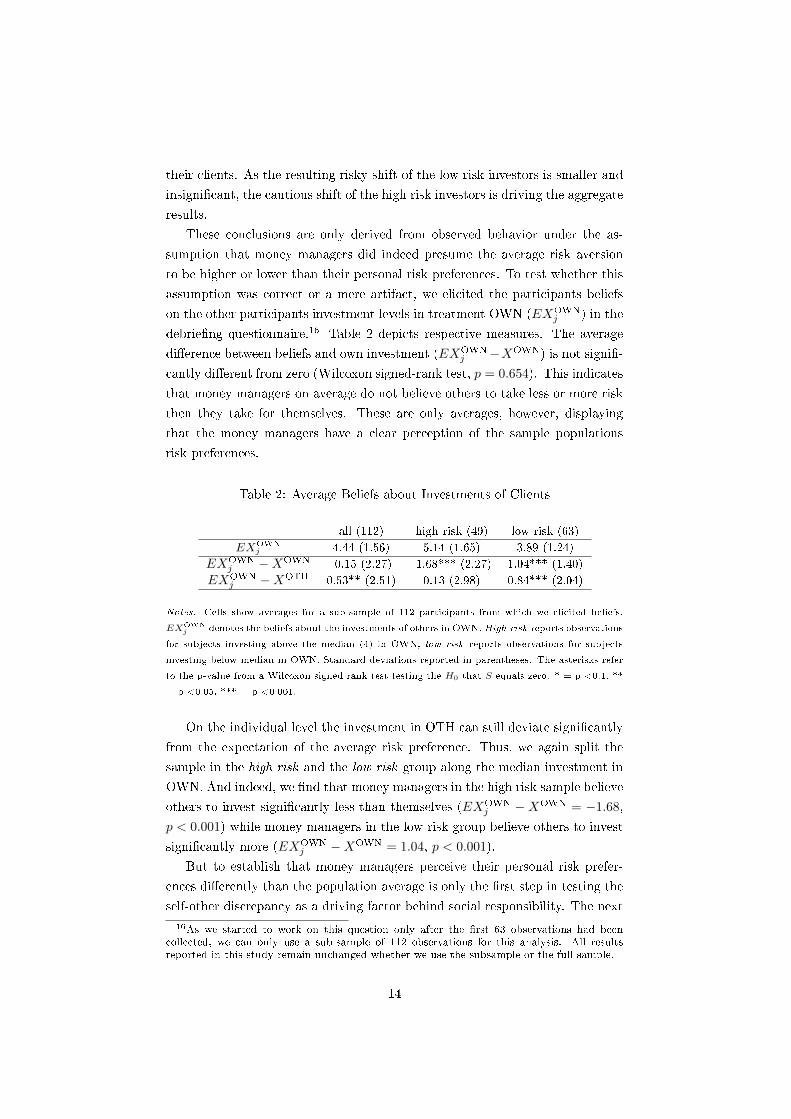
These conclusions are only derived from observed behavior under the as-

sumption that money managers did indeed presume the average risk aversion

to be higher or lower than their personal risk preferences. To test whether this

assumption was correct or a mere artifact, we elicited the participants beliefs

on the other participants investment levels in treatment OWN (EXOWNj ) in the

debrie�ng questionnaire.16 Table 2 depicts respective measures. The average

di�erence between beliefs and own investment (EXOWNj −XOWN) is not signi�-

cantly di�erent from zero (Wilcoxon signed-rank test, p = 0.654). This indicates

that money managers on average do not believe others to take less or more risk

then they take for themselves. These are only averages, however, displaying

that the money managers have a clear perception of the sample populations

risk preferences.

Table 2: Average Beliefs about Investments of Clients

all (112) high risk (49) low risk (63)

EXOWNj 4.44 (1.56) 5.14 (1.65) 3.89 (1.24)

EXOWNj −XOWN -0.15 (2.27) -1.68*** (2.27) 1.04*** (1.40)

EXOWNj −XOTH 0.53** (2.51) 0.13 (2.98) 0.84*** (2.04)

Notes. Cells show averages for a sub-sample of 112 participants from which we elicited beliefs.

EXOWNj denotes the beliefs about the investments of others in OWN. High risk reports observations

for subjects investing above the median (4) in OWN, low risk reports observations for subjects

investing below median in OWN. Standard deviations reported in parentheses. The asterisks refer

to the p-value from a Wilcoxon signed rank test testing the H0 that S equals zero. * = p <0.1, **

= p <0.05, *** = p <0.001.

On the individual level the investment in OTH can still deviate signi�cantly

from the expectation of the average risk preference. Thus, we again split the

sample in the high risk and the low risk group along the median investment in

OWN. And indeed, we �nd that money managers in the high risk sample believe

others to invest signi�cantly less than themselves (EXOWNj −XOWN = −1.68,

p < 0.001) while money managers in the low risk group believe others to invest

signi�cantly more (EXOWNj −XOWN = 1.04, p < 0.001).

But to establish that money managers perceive their personal risk prefer-

ences di�erently than the population average is only the �rst step in testing the

self-other discrepancy as a driving factor behind social responsibility. The next

16As we started to work on this question only after the �rst 63 observations had beencollected, we can only use a sub-sample of 112 observations for this analysis. All resultsreported in this study remain unchanged whether we use the subsample or the full sample.

14

step is to uncover whether investments for the clients are in line with beliefs

about what clients invest for themselves, i.e., whether EXOWNj − XOTH = 0.

Without splitting the sample, we �nd that money managers invest signi�-

cantly less for clients than what they believe clients would invest for themselves

(∆OTH = 0.53, p = 0.002). However, this result is mainly driven by the low

risk sample as we �nd the observed di�erences not to be signi�cant in the high

risk sample (EXOWNj −XOTH = 0.13, p = 0.676 ) but highly signi�cant in the

low risk sample (EXOWNj −XOTH = 0.84, p < 0.001). Thus, money managers

in the high risk group roughly invest for their clients what they believe the

clients would invest for themselves while the low risk group money managers

invest less. Overall, we can say that money managers are relatively conserva-

tive in that they invest at most what they believe the others would invest for

themselves.

Observation 3. When investing for others without payo� alignment, money

managers act according to their believed risk preferences of their clients.

The high risk money managers had indeed expected to be above the average

investment as had the low risk money managers expected to be below. More

importantly we �nd the investments in OTH not to be di�erent from what the

high risk money managers believed their investors would invest for themselves.

This again is a clear indicator for acting according to social preferences when

there are no opposing individual incentives. This is in line with results from

Bolton et al. (2015) who show that money managers act according to the clients

preferences if information about the clients preferences was revealed beforehand.

Our design allows us to compare the investment shift when the payment is

perfectly aligned and when the payment is not aligned. If the investments in

both treatments were equal yet di�erent to OWN ( SOTH = SLEA 6= 0) this

would mean that the money managers ignore their own risk preferences. We

�nd the cautious shift to be on average lower in LEA (SLEA = −0.57) than in

OTH (SOTH = −0.65), though this di�erence is not signi�cant using a Wilcoxon

signed rank test. Only for the high risk sample we �nd the shift to be weakly

signi�cant higher in OTH than in LEA. The aggregate results suggest that the

money managers ignore their own preferences to fully meet the clients needs.

Observation 4. The investment shifts in LEA and OTH are not signi�cantly

di�erent at the 5 percent signi�cance level.

This is a surprising result. The aggregate observations suggest not only

that money managers feature social preferences but also that their individual

risk preferences are overridden, once they decide for themselves and a group

of clients. To examine the origins of this, rather counter intuitive, aggregate

pattern, we look at individual behavior in the following section.

15

4.2 Responsibility weights

Apparently, in LEA the money managers deviate substantially from their own

risk preferences and act rather in line with the risk preferences of the clients.

This raises the question of how much weight is put on each of these opposing

preferences when making an investment in LEA. Our experimental design al-

lows us to model the relationship between individual risk preferences and the

perceived risk preferences of the clients by considering the link-treatment LEA;

the combination of OWN and OTH. If the money managers only care about

themselves, we would predict XOWN = XLEA independent of XOTH. Thus,

the decision re�ects the risk attitude of the decision maker only. If the money

managers only care for the clients, we would predict XLEA = XOTH indepen-

dent of XOWN. And indeed the previous section indicates that on average

XOWN > XLEA = XOTH. Hence, the average money managers take responsi-

bility for the clients and put their own needs in LEA on hold, as they are willing

to reduce the investment levels for themselves in LEA in comparison to OWN.

Whether a money managers �cares� more for himself or rather for the clients

can be inferred by estimating a responsibility weight α given by the relationship

in (1).

XLEAi = (1− αi)X

OWNi + αiX

OTHi =⇒αi =

SLEAi

SOTHi

. (1)

The interpretation is straight forward given SOTH 6= 0. For α = 0, the

money manager cares only for himself which implies that XLEA = XOWN . For

α = 1, the money manager cares only for his clients and puts his own preferences

to hold implying XLEA = XOTH . For 0 < α < 1, the money managers weights

egoistic preferences and social preferences. Suppose a money manager opts for a

cautious shift such that α = 0.70. This indicates that the money manager takes

the clients' risk preferences with a weight of 70 percent into account, and his

own risk preferences with a weight of 30 percent. Table 3 provides aggregates

for the responsibility weight α.

16

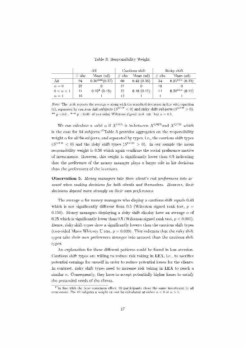
Table 3: Responsibility Weight

All Cautious shift Risky shift

# obs Mean (sd) # obs Mean (sd) # obs Mean (sd)

All 94 0.36***(0.37) 60 0.42 (0.38) 34 0.25*** (0.33)

α = 0 37 0 21 0 16 0

0 < α < 1 41 0.43* (0.18) 27 0.48 (0.17) 14 0.32*** (0.17)

α = 1 16 1 12 1 4 1

Note: The table reports the average α along with the standard deviation in line with equation

(1), separated by cautious shift subjects (SOTH < 0) and risky shift subjects (SOTH > 0).

** p <0.01, *** p <0.001 of two-sided Wilcoxon signed rank test that α = 0.5.

We can calculate a valid α if XLEA is in-between XOWNand XOTH which

is the case for 94 subjects.17Table 3 provides aggregates on the responsibility

weight α for all 94 subjects, and separated by types, i.e., the cautious shift types

(SOTH < 0) and the risky shift types (SOTH > 0). In our sample the mean

responsibility weight is 0.36 which again con�rms the social preference motive

of investments. However, this weight is signi�cantly lower than 0.5 indicating

that the preference of the money manager plays a larger role in his decisions

than the preferences of the investors.

Observation 5. Money managers take their client's risk preferences into ac-

count when making decisions for both clients and themselves. However, their

decisions depend more strongly on their own preferences.

The average α for money managers who display a cautious shift equals 0.43

which is not signi�cantly di�erent from 0.5 (Wilcoxon signed rank test, p =

0.150). Money managers displaying a risky shift display have an average α of

0.25 which is signi�cantly lower than 0.5 (Wilcoxon signed rank test, p < 0.001).

Hence, risky shift types show a signi�cantly lowerα than the cautious shift types

(two-sided Mann Whitney U test, p = 0.039). This indicates that the risky shift

types take their own preferences stronger into account than the cautious shift

types.

An explanation for these di�erent patterns could be found in loss aversion.

Cautious shift types are willing to reduce risk taking in LEA, i.e., to sacri�ce

potential earnings for oneself in order to reduce potential losses for the clients.

In contrast, risky shift types need to increase risk taking in LEA to reach a

similar α. Consequently, they have to accept potentially higher losses to satisfy

the pretended needs of the clients.

17In line with the false consensus e�ect, 39 participants chose the same investment in alltreatments. For 42 subjects a weight cannot be calculated as either α < 0 or α > 1.

17

5 Discussion and Conclusion

We study the e�ects of responsibility in risky decision making, using a one-

shot Gneezy and Potters (1997) investment game while controlling for confound-

ing e�ects detected in the literature. First, in line with responsibility alleviation,

we �nd a signi�cant cautious shift in risky decisions for others, irrespective of

whether the decision makers payo�s are perfectly aligned with the clients or

independent. Second, in line with the self-other-distance theory, we �nd that

money managers invest in line with what they believe others would like to invest

for themselves (in line with Bolton et al., 2015). In particular, money makers

exhibiting low risk aversion make rather conservative investments for others, re-

sulting in a cautious shift, while highly risk averse money managers take higher

risks for their clients, resulting in a risky shift. Third, using a responsibility

weighting model we �nd that cautious shift types take own preferences and the

preferences of the clients about equally into account when making investment

decisions in LEA. However, risky shift types overweight their own preferences as

a higher weight for the clients would increase their own risk taking and potential

losses.

But how can we explain the mixed results in the literature? In the following,

we provide some suggestions in line with our results.

Loss aversion for more than one other. Previous studies have reported a

risky shift and argue that reduced loss aversion due to a higher social distance

explains the risky shift (e.g., Andersson et al., forthcoming). Thus, a reason

for the di�erence in results might be that the argument holds if deciding for

one client only. But it might be that aggregated loss aversion for six clients is

greater than loss aversion for oneself leading to a cautious shift.18 Hence, we

ran further experiments in which the money manager invests for one client only

as a robustness check (see section C in the online supplement). The results

provide no indication for a risky shift either. We rather �nd that the results

are qualitatively equal to the results in the experiments with six clients. We

conclude that the level of responsibility does not alter our �ndings.

Ambiguity Aversion. While money managers might know their own pref-

erences, they are uncertain about the clients' preferences; in particular when

estimating the preferences of six clients. This creates an ambiguous situation

when deciding for others in contrast to when deciding for oneself. From that

point of view, our results are in line with ambiguity aversion as subjects take less

risk in a situation with higher ambiguity (e.g., Trautmann and Van De Kuilen,

forthcoming). This is even ampli�ed as in the within-subject design subjects are

18We thank participants from the ESA North American Meeting 2014 for raising this argu-ment.

18

able to compare decisions for others and for themselves in line with comparative

ignorance (Fox and Tversky, 1995).

Risk attitude of the population. The conclusions so far are based on aggregate

results only, as is the case in the previous literature. Due to our within-subject

design we are able to take the relative risk attitudes of the money manager

into account. We �nd that the results are driven by the relatively risk seeking

subjects, while for the relatively risk averse subjects we �nd rather a risky shift.

Given our sample, the aggregate result of a cautious shift is driven by the group

of high risk money managers. But any study with a rather risk averse subject

pool would �nd an aggregate risky shift, of course. Hence, di�erences to for

instance Andersson et al. (forthcoming) might be due to the fact that their

subject pool is taken from the general Danish population which has been found

to be more risk averse than the common student population (von Gaudecker

et al., 2012).19

Social Distance. Among others, Eriksen and Kvaløy (2010) report that hy-

pothetical decision making for others - the most extreme social distance - leads

to higher risk taking in comparison to a situation with monetary consequences.

Thus, experiments with higher social distance, as is the case for internet ex-

periments in as compared to laboratory experiments, might lead to higher risk

taking for others.On the other hand our experimental design allows the poten-

tial money managers to put themselves into the position of the clients as with

high probability the money manager becomes a client. This might lead to a

higher empathy for the others leading to a rather cautious shift (as in the equal

opportunity mode treatment in Bolton and Ockenfels, 2006).

Domains. The results from the literature suggest that the domain of the

lotteries plays a relevant role. Lotteries in the loss domain or in the mixed

domain seem to support a risky shift while lotteries in the gain domain support

a cautious shift Pahlke et al. (e.g., 2012). In the Gneezy and Potters (1997)

investment game, however, we cannot control the subject's perception of the

game as we have no record of the editing phase (Kahneman and Tversky, 1979).

When the endowment is integrated, the decision takes place in the gain domain

only (9 + 2.5X vs. 9 − X). When the endowment is segregated, the decision

takes place in the mixed domain (2.5X vs. −X). Our results point to the

former as we provide integrated outcomes on the decision screen which fosters

a cautious shift (see section E in the online supplement).

What drives investments when payments are perfectly aligned (LEA): Ego-

istic preferences or social preferences? Unfortunately, the literature so far has

19Another reason might be that the self-other distance is higher in internet experimentsthan in the laboratory. In the extreme case, online subjects might perceive the situation ashypothetical, which would lead to higher risk taking (Harrison, 2006; Eriksen and Kvaløy,2010).

19

not considered the link between LEA and OWN on the one hand, and LEA and

OTH on the other hand. These links, however, are quite important to answer

the question, as it combines decision making for oneself only and decision mak-

ing for others only in one decision. On average, we observe a cautious shift in

LEA and OTH which is smaller in LEA than in OTH. Hence, in LEA the social

preferences play a role but the money managers cannot be expected to fully

disregard their own preferences. While this consideration is straight forward,

we are (to the best of our knowledge) the �rst to directly compare these two

situations. Using the decisions in OTH and in OWN as reference points, we are

able to construct a weighed risk preference model allowing us to determine the

individual responsibility weight of our participants. On average the money man-

agers take not only their own risk preferences (egoistic preferences) into account

but also the risk preferences of the clients (social risk preferences). Though they

seem to weight their egoistic preferences stronger than the social preferences.

Casually speaking, in our experiments decisions in LEA depend on average by

about 36 percent on social preferences and by 64 percent on egoistic preferences.

This e�ect is even stronger for the risky-shift managers. They have to accept

higher losses for the good of the others while the cautious-shift managers have

to only sacri�ce potential earnings.

References

Agranov, M., Bisin, A., Schotter, A., 2014. An experimental study of the im-

pact of competition for other people's money: the portfolio manager market.

Experimental Economics, 564�585.

Albrecht, K., Volz, K. G., Sutter, M., Laibson, D. I., Von Cramon, D. Y., 2011.

What is for me is not for you: brain correlates of intertemporal choice for self

and other. Social Cognitive and A�ective Neuroscience 2, 218�225.

Allen, F., Gale, D., 2000. Bubbles and crises. The Economic Journal 110 (460),

236�255.

Allen, F., Gorton, G., 1993. Churning bubbles. The Review of Economic Studies

60 (4), 813�836.

Andersson, O., Holm, H. J., Tyran, J.-R., Wengström, E., forthcoming. Deciding

for others reduces loss aversion. Management Science.

Beisswanger, A. H., Stone, E. R., Hupp, J. M., Allgaier, L., 2003. Risk taking

in relationships: Di�erences in deciding for oneself versus for a friend. Basic

and Applied Social Psychology 25 (2), 121�135.

20

Berkowitz, L., Lutterman, K. G., 1968. The traditional socially responsible per-

sonality. Public Opinion Quarterly 32 (2), 169�185.

Bolton, G. E., Ockenfels, A., 2000. Erc: A theory of equity, reciprocity, and

competition. American Economic Review 90 (1), 166�193.

Bolton, G. E., Ockenfels, A., 2006. Inequality aversion, e�ciency, and maximin

preferences in simple distribution experiments: comment. The American eco-

nomic review 96 (5), 1906�1911.

Bolton, G. E., Ockenfels, A., 2010. Betrayal aversion: Evidence from brazil,

china, oman, switzerland, turkey, and the united states: Comment. The

American Economic Review 100 (1), 628�633.

Bolton, G. E., Ockenfels, A., Stauf, J., 2015. Social responsibility promotes

conservative risk behavior. European Economic Review 74 (0), 109 � 127.

Chakravarty, S., Harrison, G. W., Haruvy, E. E., Rutström, E. E., 2011. Are you

risk averse over other people's money? Southern Economic Journal 77 (4),

901�913.

Charness, G., 2000. Responsibility and e�ort in an experimental labor market.

Journal of Economic Behavior & Organization 42 (3), 375�384.

Charness, G., Gneezy, U., 2012. Strong evidence for gender di�erences in risk

taking. Journal of Economic Behavior & Organization 83 (1), 50�58.

Charness, G., Gneezy, U., Imas, A., 2013. Experimental methods: Eliciting risk

preferences. Journal of Economic Behavior & Organization 87, 43�51.

Charness, G., Jackson, M. O., 2009. The role of responsibility in strategic risk-

taking. Journal of Economic Behavior & Organization 69 (3), 241�247.

Charness, G., Rabin, M., 2002. Understanding social preferences with simple

tests. The Quarterly Journal of Economics 117 (3), 817�869.

Charness, G., Rabin, M., 2005. Expressed preferences and behavior in experi-

mental games. Games and Economic Behavior 53 (2), 151�169.

Cheung, S. L., Coleman, A., 2014. Relative performance incentives and price

bubbles in experimental asset markets. Southern Economic Journal 81 (2),

345�363.

Cvetkovich, G., 1972. E�ects of sex on decision policies used for self and decision

policies used for other persons. Psychonomic Science 26 (6), 319�320.

21

Dohmen, T., Falk, A., Hu�man, D., Sunde, U., Schupp, J., Wagner, G. G.,

2011. Individual risk attitudes: Measurement, determinants, and behavioral

consequences. Journal of the European Economic Association 9 (3), 522�550.

Eckel, C. C., Grossman, P. J., 2008a. Forecasting risk attitudes: An experi-

mental study using actual and forecast gamble choices. Journal of Economic

Behavior & Organization 68 (1), 1�17.

Eckel, C. C., Grossman, P. J., 2008b. Men, women and risk aversion: Experi-

mental evidence. Handbook of experimental economics results 1 (7), 1061�73.

Eriksen, K. W., Kvaløy, O., 2010. Myopic investment management. Review of

Finance 14 (3), 521�542.

Fehr, E., Schmidt, K. M., 1999. A theory of fairness, competition, and cooper-

ation. The Quarterly Journal of Economics 114 (3), 817�868.

Fischbacher, U., 2007. z-tree: Zurich toolbox for ready-made economic experi-

ments. Experimental Economics 10 (2), 171�178.

Fox, C. R., Tversky, A., 1995. Ambiguity aversion and comparative ignorance.

The Quarterly Journal of Economics 110 (3), 585�603.

Fudenberg, D., Levine, D. K., 2012. Fairness, risk preferences and independence:

Impossibility theorems. Journal of Economic Behavior & Organization 81 (2),

606�612.

Garcia-Retamero, R., Galesic, M., 2012. Doc, what would you do if you were

me? on self�other discrepancies in medical decision making. Journal of Ex-

perimental Psychology: Applied 18 (1), 38.

Gneezy, U., Potters, J., 1997. An experiment on risk taking and evaluation

periods. The Quarterly Journal of Economics 112 (2), 631�645.

Harbaugh, W. T., Krause, K., Vesterlund, L., 2010. The fourfold pattern of

risk attitudes in choice and pricing tasks. The Economic Journal 120 (545),

595�611.

Harrison, G. W., 2006. Hypothetical bias over uncertain outcomes. In: List,

J. A. (Ed.), Using epxperimental methods in environmental and resource eco-

nomics. Northampton. MA: Elgar, pp. 41�69.

Holt, C. A., Laury, S. K., 2002. Risk aversion and incentive e�ects. American

Economic Review 92 (5), 1644�1655.

Holt, C. A., Laury, S. K., 2005. Risk aversion and incentive e�ects: New data

without order e�ects. The American Economic Review 95 (3), 902�904.

22

Hsee, C. K., Weber, E. U., 1997. A fundamental prediction error: Self�others

discrepancies in risk preference. Journal of Experimental Psychology: General

126 (1), 45.

Huber, J., Kirchler, M., Stöckl, T., 2010. The hot hand belief and the gambler's

fallacy in investment decisions under risk. Theory and Decision 68 (4), 445�

462.

Humphrey, S. J., Renner, E., 2011. The social costs of responsibility, ceDEx

discussion paper series.

Kahneman, D., Tversky, A., 1979. Prospect theory: An analysis of decision

under risk. Econometrica: Journal of the Econometric Society, 263�291.

Kleinlercher, D., Huber, J., Kirchler, M., 2014. The impact of di�erent incentive

schemes on asset prices. European Economic Review 68, 137�150.

Leuermann, A., Roth, B., 2012. Does good advice come cheap? on the assess-

ment of risk preferences in the lab and in the �eld. Tech. rep., SOEPpapers

on Multidisciplinary Panel Data Research.

Montinari, N., Rancan, M., 2013. Social preferences under risk: the role of

social distance, jena Economic Research Papers 2013-50, Friedrich-Schiller-

University Jena, Max-Planck-Institute of Economics.

Noussair, C. N., Trautmann, S. T., Van de Kuilen, G., 2014. Higher order risk

attitudes, demographics, and �nancial decisions. The Review of Economic

Studies 81 (1), 325�355.

Pahlke, J., Strasser, S., Vieider, F. M., 2012. Risk-taking for others under ac-

countability. Economics Letters 114 (1), 102�105.

Pollmann, M. M., Potters, J., Trautmann, S. T., 2014. Risk taking by agents:

The role of ex-ante and ex-post accountability. Economics Letters 123 (3),

387�390.

Polman, E., 2012. Self�other decision making and loss aversion. Organizational

Behavior and Human Decision Processes 119 (2), 141�150.

Reynolds, D. B., Joseph, J., Sherwood, R., 2009. Risky shift versus cautious

shift: determining di�erences in risk taking between private and public man-

agement decision-making. Journal of Business & Economics Research 7 (1).

Robin, S., Straznicka, K., Villeval, M. C., 2011. Bubbles and incentives. In:

Journées de l'Association Française d'Economie Expérimentale (ASFEE),

Université des Antilles et de la Guyane, Schoelcher, Martinique.

23

Ross, L., Greene, D., House, P., 1977. The "false consensus e�ect": An ego-

centric bias in social perception and attribution processes. Journal of Exper-

imental Social Psychology 13 (3), 279�301.

Stone, E. R., Allgaier, L., 2008. A social values analysis of self�other di�erences

in decision making involving risk. Basic and Applied Social Psychology 30 (2),

114�129.

Stoner, J. A. F., 1961. A comparison of individual and group decisions involving

risk. Ph.D. thesis, Massachusetts Institute of Technology.

Sutter, M., 2009. Individual behavior and group membership: Comment. The

American Economic Review 99 (5), 2247�2257.

Swalm, R. O., 1966. Utility theory-insights into risk taking. Harvard Business

Review 44 (6), 123�136.

Trautmann, S., Van De Kuilen, G., forthcoming. Ambiguity attitudes. In:

Keren, G., Wu, G. (Eds.), Blackwell Handbook of Judgment and Decision

Making. Blackwell.

Trautmann, S. T., Vieider, F. M., 2012. Social in�uences on risk attitudes:

Applications in economics. In: Handbook of risk theory. Springer, pp. 575�

600.

Trope, Y., Liberman, N., 2010. Construal-level theory of psychological distance.

Psychological Review 117 (2), 440.

Ubel, P. A., Angott, A. M., Zikmund-Fisher, B. J., 2011. Physicians recom-

mend di�erent treatments for patients than they would choose for themselves.

Archives of Internal Medicine 171 (7), 630�634.

Viscusi, W. K., Magat, W. A., Huber, J., 1987. An investigation of the ratio-

nality of consumer valuations of multiple health risks. The RAND Journal of

Economics, 465�479.

von Gaudecker, H.-M., van Soest, A., Wengström, E., 2012. Experts in experi-

ments. Journal of Risk and Uncertainty 45 (2), 159�190.

Wray, L. D., Stone, E. R., 2005. The role of self-esteem and anxiety in decision

making for self versus others in relationships. Journal of Behavioral Decision

Making 18 (2), 125�144.

24

Online Supplement

A Pool Data

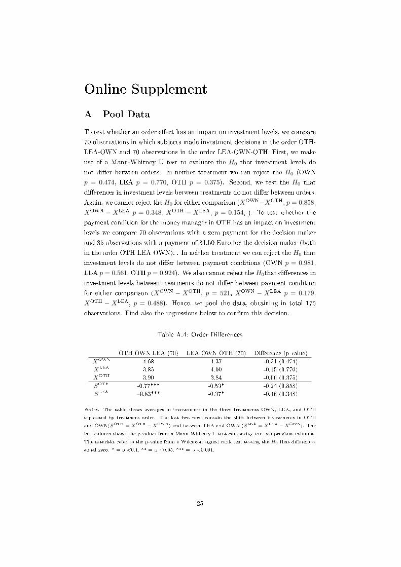
To test whether an order e�ect has an impact on investment levels, we compare

70 observations in which subjects made investment decisions in the order OTH-

LEA-OWN and 70 observations in the order LEA-OWN-OTH. First, we make

use of a Mann-Whitney U test to evaluate the H0 that investment levels do

not di�er between orders. In neither treatment we can reject the H0 (OWN

p = 0.474, LEA p = 0.770, OTH p = 0.375). Second, we test the H0 that

di�erences in investment levels between treatments do not di�er between orders.

Again, we cannot reject theH0 for either comparison (XOWN−XOTH, p = 0.858,

XOWN − XLEA p = 0.348, XOTH − XLEA, p = 0.154, ). To test whether the

payment condition for the money manager in OTH has an impact on investment

levels we compare 70 observations with a zero payment for the decision maker

and 35 observations with a payment of 31.50 Euro for the decision maker (both

in the order OTH-LEA-OWN). . In neither treatment we can reject the H0 that

investment levels do not di�er between payment conditions (OWN p = 0.981,

LEA p = 0.561, OTH p = 0.924). We also cannot reject theH0that di�erences in

investment levels between treatments do not di�er between payment condition

for either comparison (XOWN − XOTH, p = 521, XOWN − XLEA p = 0.179,

XOTH − XLEA, p = 0.488). Hence, we pool the data, obtaining in total 175

observations. Find also the regressions below to con�rm this decision.

Table A.4: Order Di�erences

OTH-OWN-LEA (70) LEA-OWN-OTH (70) Di�erence (p-value)

XOWN 4.68 4.37 -0.31 (0.474)

XLEA 3.85 4.00 -0.15 (0.770)

XOTH 3.90 3.84 -0.06 (0.375)

SOTH -0.77*** -0.53* -0.24 (0.858)

SLEA �0.83*** -0.37* -0.46 (0.348)

Notes. The table shows averages in investments in the three treatments OWN, LEA, and OTH

separated by treatment order. The last two rows contain the shift between investments in OTH

and OWN(SOTH = XOTH −XOWN) and between LEA and OWN (SLEA = XLEA −XOWN). The

last column shows the p-values from a Mann-Whitney U test comparing the two previous columns.

The asterisks refer to the p-value from a Wilcoxon signed rank test testing the H0 that di�erences

equal zero. * = p <0.1, ** = p <0.05, *** = p <0.001.

25

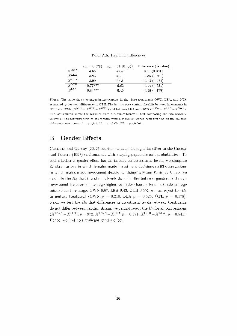
Table A.5: Payment di�erences

πm = 0 (70) πm = 31.50 (35) Di�erence (p-value)

XOWN 4.68 4.65 0.03 (0.981)

XLEA 3.85 4.21 -0.36 (0.561)

XOTH 3.90 4.03 -0.13 (0.924)

SOTH -0.77*** -0.63 -0.14 (0.521)

SLEA -0.83*** -0.45 -0.38 (0.179)

Notes. The table shows averages in investments in the three treatments OWN, LEA, and OTH

separated by payment di�erences in OTH. The last two rows contain the shift between investments in

OTH and OWN (SOTH = XOTH−XOWN) and between LEA and OWN (SLEA = XLEA−XOWN).

The last column shows the p-values from a Mann-Whitney U test comparing the two previous

columns. The asterisks refer to the p-value from a Wilcoxon signed rank test testing the H0 that

di�erences equal zero. * = p <0.1, ** = p <0.05, *** = p <0.001.

B Gender E�ects

Charness and Gneezy (2012) provide evidence for a gender e�ect in the Gneezy

and Potters (1997) environment with varying payments and probabilities. To

test whether a gender e�ect has an impact on investment levels, we compare

82 observations in which females made investment decisions to 93 observations

in which males made investment decisions. Usingf a Mann-Whitney U test we

evaluate the H0 that investment levels do not di�er between gender. Although

investment levels are on average higher for males than for females (male average

minus female average: OWN 0.67, LEA 0.43, OTH 0.55), we can reject the H0

in neither treatment (OWN p = 0.210, LEA p = 0.525, OTH p = 0.178).

Next, we test the H0 that di�erences in investment levels between treatments

do not di�er between gender. Again, we cannot reject the H0 for all comparisons

(XOWN−XOTH, p = 972, XOWN−XLEA p = 0.371, XOTH−XLEA, p = 0.541).

Hence, we �nd no signi�cant gender e�ect.

26

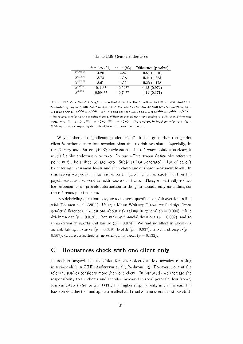
Table B.6: Gender di�erences

females (81) male (93) Di�erence (p-value)

XOWN 4.20 4.87 -0.67 (0.210)

XLEA 3.75 4.18 -0.44 (0.525)

XOTH 3.61 4.16 -0.55 (0.178)

SOTH -0.44** -0.69** 0.25 (0.972)

SLEA -0.59*** -0.70** 0.11 (0.371)

Notes. The table shows averages in investments in the three treatments OWN, LEA, and OTH

separated by payment di�erences in OTH. The last two rows contain the shift between investments in

OTH and OWN (SOTH = XOTH−XOWN) and between LEA and OWN (SLEA = XLEA−XOWN).

The asterisks refer to the p-value from a Wilcoxon signed rank test testing the H0 that di�erences

equal zero. * = p <0.1, ** = p <0.05, *** = p <0.001. The p-values in brackets refer to a Mann

Whitney U test comparing the unit of interest across treatments.

Why is there no signi�cant gender e�ect? It is argued that the gender

e�ect is rather due to loss aversion than due to risk aversion. Especially, in

the Gneezy and Potters (1997) environment the reference point is unclear; it

might be the endowment or zero. In our z-Tree screen design the reference

point might be shifted toward zero. Subjects �rst generated a list of payo�s

by entering investment levels and then chose one of these investment levels. In

this screen we provide information on the payo� when successful and on the

payo� when not successful; both above or at zero. Thus, we virtually reduce

loss aversion as we provide information in the gain domain only and, thus, set

the reference point to zero.

In a debrie�ng questionnaire, we ask several questions on risk aversion in line

with Dohmen et al. (2011). Using a Mann-Whitney U test, we �nd signi�cant

gender di�erences in questions about risk taking in general (p = 0.004), while

driving a car (p = 0.019), when making �nancial decisions (p = 0.002), and to

some extent in sports and leisure (p = 0.074). We �nd no e�ect in questions

on risk taking in career (p = 0.319), health (p = 0.937), trust in strangers(p =

0.567), or in a hypothetical investment decision (p = 0.132).

C Robustness check with one client only

It has been argued that a decision for others decreases loss aversion resulting

in a risky shift in OTH (Andersson et al., forthcoming). However, none of the

relevant studies considers more than one client. In our study we increase the

responsibility to six clients and thereby increase the total potential loss from 9

Euro in OWN to 54 Euro in OTH. The higher responsibility might increase the

loss aversion due to a multiplicative e�ect and results in an overall cautious shift.

27

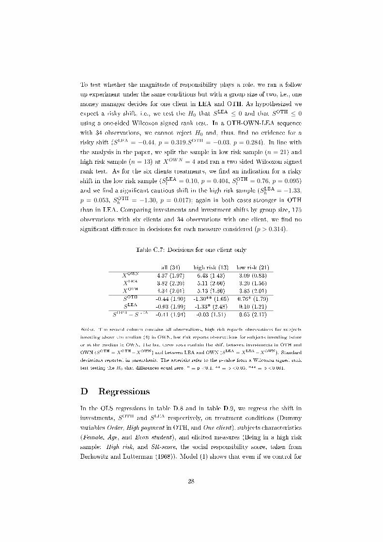
To test whether the magnitude of responsibility plays a role, we ran a follow

up experiment under the same conditions but with a group size of two, i.e., one

money manager decides for one client in LEA and OTH. As hypothesized we

expect a risky shift, i.e., we test the H0 that SLEA ≤ 0 and that SOTH ≤ 0

using a one-sided Wilcoxon signed rank test. In a OTH-OWN-LEA sequence

with 34 observations, we cannot reject H0 and, thus, �nd no evidence for a

risky shift (SLEA = −0.44, p = 0.319,SOTH = −0.03, p = 0.284). In line with

the analysis in the paper, we split the sample in low risk sample (n = 21) and

high risk sample (n = 13) at XOWN = 4 and ran a two sided Wilcoxon signed

rank test. As for the six clients treatments, we �nd an indication for a risky

shift in the low risk sample (SLEAl = 0.10, p = 0.404, SOTHl = 0.76, p = 0.095)

and we �nd a signi�cant cautious shift in the high risk sample (SLEAh = −1.33,

p = 0.053, SOTHh = −1.30, p = 0.017); again in both cases stronger in OTH

than in LEA. Comparing investments and investment shifts by group size, 175

observations with six clients and 34 observations with one client, we �nd no

signi�cant di�erence in decisions for each measure considered (p > 0.314).

Table C.7: Decisions for one client only

all (34) high risk (13) low risk (21)

XOWN 4.37 (1.97) 6.43 (1.43) 3.09 (0.83)

XLEA 3.82 (2.20) 5.11 (2.60) 3.20 (1.56)

XOTH 4.34 (2.01) 5.13 (1.80) 3.85 (2.01)

SOTH -0.44 (1.90) -1.30** (1.65) 0.76* (1.79)

SLEA -0.03 (1.99) -1.33* (2.48) 0.10 (1.21)

SOTH − SLEA -0.41 (1.94) -0.03 (1.51) 0.65 (2.17)

Notes. The second column contains all observations, high risk reports observations for subjects

investing above the median (4) in OWN, low risk reports observations for subjects investing below

or at the median in OWN. The last three rows contain the shift between investments in OTH and

OWN (SOTH = XOTH−XOWN) and between LEA and OWN (SLEA = XLEA−XOWN). Standard

deviations reported in parenthesis. The asterisks refer to the p-value from a Wilcoxon signed rank

test testing the H0 that di�erences equal zero. * = p <0.1, ** = p <0.05, *** = p <0.001.

D Regressions

In the OLS regressions in table D.8 and in table D.9, we regress the shift in

investments, SOTH and SLEA respectively, on treatment conditions (Dummy

variables Order, High payment in OTH, and One client), subjects characteristics

(Female, Age, and Econ student), and elicited measures (Being in a high risk

sample: High risk, and SR-score, the social responsibility score, taken from

Berkowitz and Lutterman (1968)). Model (1) shows that even if we control for

28

treatment conditions we �nd the constant to be signi�cantly negative, which is

in line with non-parametric considerations in section C and section A. In model

(2) and model (3) we see, however, that the relatively risk seeking subjects drive

the cautious shift as the High risk coe�cient is negative and highly signi�cant.

In line with section B we �nd no gender e�ect. Finally, we elicited the SR-score

to show that social responsible subjects act rather in line with responsibility

alleviation. However, we �nd no correlation with the dependent variables and

we also �nd no indication that subjects who score high on the SR-score act more

in line with what they think the clients would do for themselves.

29

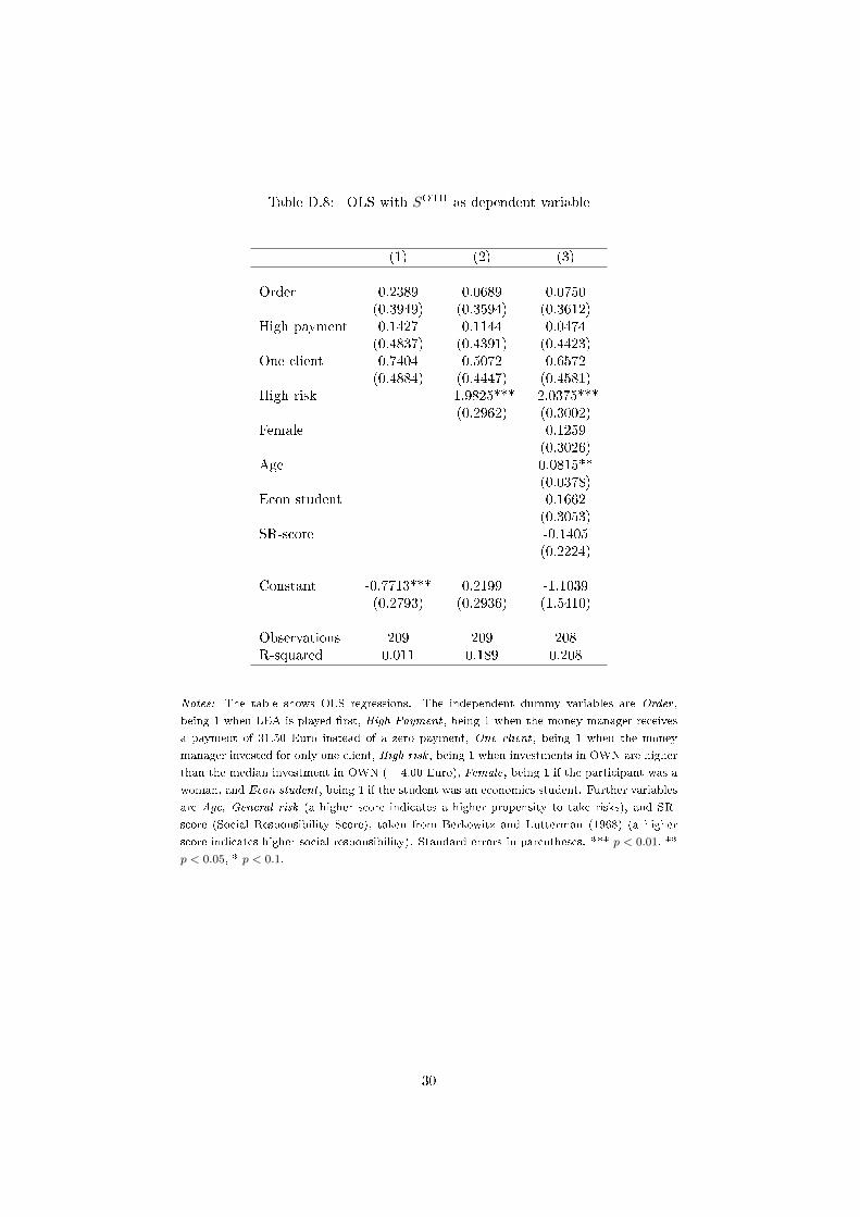
Table D.8: OLS with SOTH as dependent variable

(1) (2) (3)

Order 0.2389 0.0689 0.0750(0.3949) (0.3594) (0.3612)

High payment 0.1427 0.1144 0.0474(0.4837) (0.4391) (0.4423)

One client 0.7404 0.5072 0.6572(0.4884) (0.4447) (0.4581)

High risk -1.9825*** -2.0375***(0.2962) (0.3002)

Female 0.1259(0.3026)

Age 0.0815**(0.0378)

Econ student 0.1662(0.3053)

SR-score -0.1405(0.2224)

Constant -0.7713*** 0.2199 -1.1039(0.2793) (0.2936) (1.5410)

Observations 209 209 208R-squared 0.011 0.189 0.208

Notes: The table shows OLS regressions. The independent dummy variables are Order ,

being 1 when LEA is played �rst, High Payment , being 1 when the money manager receives

a payment of 31.50 Euro instead of a zero payment, One client , being 1 when the money

manager invested for only one client, High risk , being 1 when investments in OWN are higher

than the median investment in OWN (= 4.00 Euro), Female, being 1 if the participant was a

woman, and Econ student , being 1 if the student was an economics student. Further variables

are Age, General risk (a higher score indicates a higher propensity to take risks), and SR-

score (Social Responsibility Score), taken from Berkowitz and Lutterman (1968) (a higher

score indicates higher social responsibility). Standard errors in parentheses. *** p < 0.01, **

p < 0.05, * p < 0.1.

30

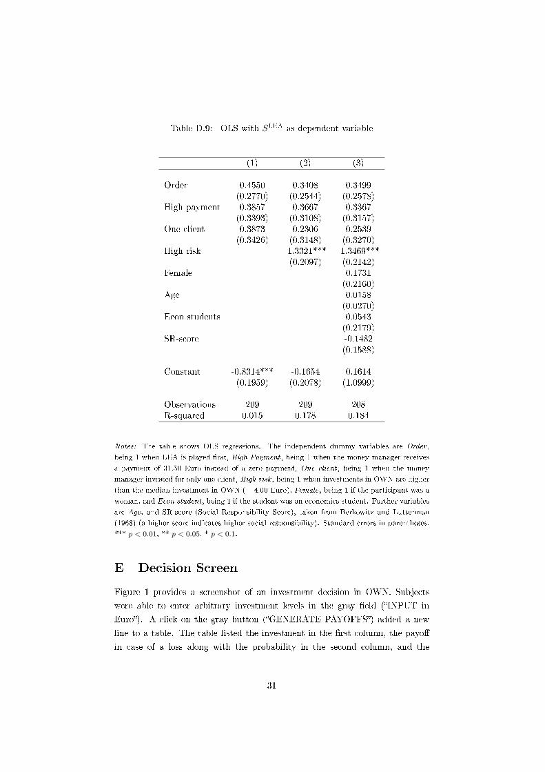
Table D.9: OLS with SLEA as dependent variable

(1) (2) (3)

Order 0.4550 0.3408 0.3499(0.2770) (0.2544) (0.2578)

High payment 0.3857 0.3667 0.3367(0.3393) (0.3108) (0.3157)

One client 0.3873 0.2306 0.2539(0.3426) (0.3148) (0.3270)

High risk -1.3321*** -1.3469***(0.2097) (0.2142)

Female 0.1731(0.2160)

Age 0.0158(0.0270)

Econ students 0.0543(0.2179)

SR-score -0.1482(0.1588)

Constant -0.8314*** -0.1654 0.1614(0.1959) (0.2078) (1.0999)

Observations 209 209 208R-squared 0.015 0.178 0.184

Notes: The table shows OLS regressions. The independent dummy variables are Order ,

being 1 when LEA is played �rst, High Payment , being 1 when the money manager receives

a payment of 31.50 Euro instead of a zero payment, One client , being 1 when the money

manager invested for only one client, High risk , being 1 when investments in OWN are higher

than the median investment in OWN (= 4.00 Euro), Female, being 1 if the participant was a

woman, and Econ student , being 1 if the student was an economics student. Further variables

are Age, and SR-score (Social Responsibility Score), taken from Berkowitz and Lutterman

(1968) (a higher score indicates higher social responsibility). Standard errors in parentheses.

*** p < 0.01, ** p < 0.05, * p < 0.1.

E Decision Screen

Figure 1 provides a screenshot of an investment decision in OWN. Subjects

were able to enter arbitrary investment levels in the gray �eld (�INPUT in

Euro�). A click on the gray button (�GENERATE PAYOFFS�) added a new

line to a table. The table listed the investment in the �rst column, the payo�

in case of a loss along with the probability in the second column, and the

31

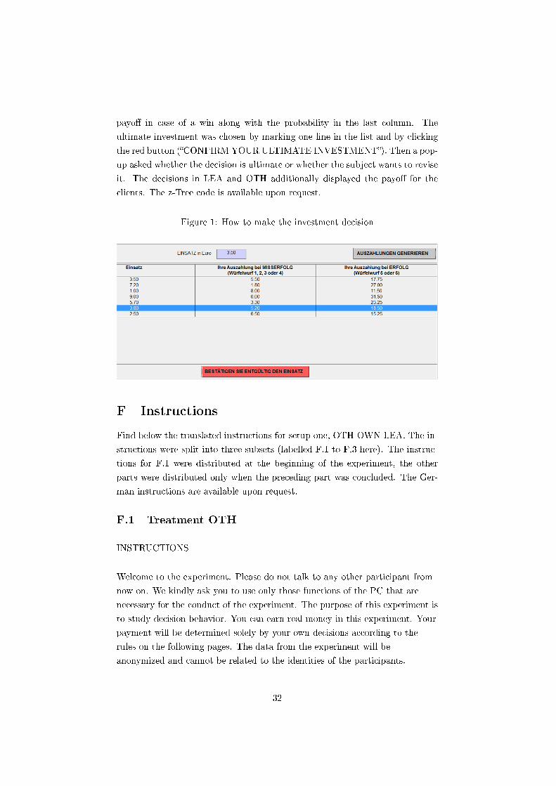
payo� in case of a win along with the probability in the last column. The

ultimate investment was chosen by marking one line in the list and by clicking

the red button (�CONFIRM YOUR ULTIMATE INVESTMENT�). Then a pop-

up asked whether the decision is ultimate or whether the subject wants to revise

it. The decisions in LEA and OTH additionally displayed the payo� for the

clients. The z-Tree code is available upon request.

Figure 1: How to make the investment decision

F Instructions

Find below the translated instructions for setup one, OTH-OWN-LEA. The in-

structions were split into three subsets (labelled F.1 to F.3 here). The instruc-

tions for F.1 were distributed at the beginning of the experiment, the other

parts were distributed only when the preceding part was concluded. The Ger-

man instructions are available upon request.

F.1 Treatment OTH

INSTRUCTIONS

Welcome to the experiment. Please do not talk to any other participant from

now on. We kindly ask you to use only those functions of the PC that are

necessary for the conduct of the experiment. The purpose of this experiment is

to study decision behavior. You can earn real money in this experiment. Your

payment will be determined solely by your own decisions according to the

rules on the following pages. The data from the experiment will be

anonymized and cannot be related to the identities of the participants.

32

Neither the other participants nor the experimenter will �nd out which choices

you have made and how much you have earned during the experiment.

SUB EXPERIMENTS

You will participate in three independent sub experiments followed by a short

questionnaire. For each sub experiment you receive a new set of instructions.

Of the three sub experiments only one will be paid out at the end of the

experiment. The payo� relevant experiment will be randomly determined by

the roll of a die.

EXPERIMENT 1

Groups - At the begin of the experiments you will be randomly organized in

groups of seven participants. Your group a�liation has no impact on your tasks

or your payment.

Role - In this part participants are either active or passive members. In each

group there is only one active member. This member decides for all other six

members and, thereby, determines their payo�. The active group member will

randomly be determined at the end of the experiment. First, all participants

decide as the active member for all other group members. At the end of the

experiment the real active member will be determined and his decision will be

implemented.

Task - In the following your decision as an active member will be explained.

The passive members receive 9 Euro each. You now decide for each of the

other members how much of their 9 Euro to invest in a risky project. The

investment is the same for each passive group member, i.e., when you invest a

certain amount then you invest this amount for each passive group member.

The remaining amount (9 Euro - Investment) will be paid out to each passive

member independent of the project's success.

The project is either a success or a failure. In case of a success each passive

member gets her invested amount back and in addition receives 2.5 times of the

investment as a gain:

Payment in case of success = 9 + 2.5×Investment.

In case of a failure the investment is lost:

Payment in case of failure = 9−Investment.

Whether the project is successful will be determined by the throw of a six-sided

die at the end of the experiment. In case of a �ve or six, the project is a success,

in case of a one, two, three or four the project is a failure. The probability of

success is therefore 33.33%.

The active member receives no payo� in this sub experiment..

33

Procedure - Details on how to enter the investments - calculation of potential

payments, �elds of entry, etc - will be displayed on the upper part of your

screen once the experiment has started.

F.2 Treatment OWN

EXPERIMENT 2

In this experiment you decide only for yourself, independent of the other par-

ticipants. You receive 9 Euro and decide how much of their 9 Euro to invest in

a risky project. The remaining amount (9 Euro - Investment) will be paid out

independent of the project's success.

The project is either a success or a failure. In case of a success You will get

your invested amount back and in addition receive 2.5 times of the investment

as a gain:

Payment in case of success = 9 + 2.5×Investment.

In case of a failure the investment is lost:

Payment in case of failure = 9−Investment.

Whether the project is successful will be determined by the throw of a six-sided

die at the end of the experiment. In case of a �ve or six, the project is a success,

in case of a one, two, three or four the project is a failure. The probability of

success is therefore 33.33%.

Procedure - Details on how to enter the investments - calculation of potential

payments, �elds of entry, etc - will be displayed on the upper part of your

screen once the experiment has started.

F.3 Treatment LEA

EXPERIMENT 3

Groups - At the begin of the experiments you will be randomly organized in

groups of seven participants. You will be regrouped, this means that the group

members are not the same as in the �rst sub experiment. Your group a�liation

has no impact on your tasks or your payment.

Role - In this part participants are either active or passive members. In each

group there is only one active member. This member decides for all other six

members and, there by, determines their payo�. The active group member will

randomly be determined at the end of the experiment. First, all participants

decide as the active member for all other group members. At the end of the

experiment the real active member will be determined and his decision will be

implemented.

34

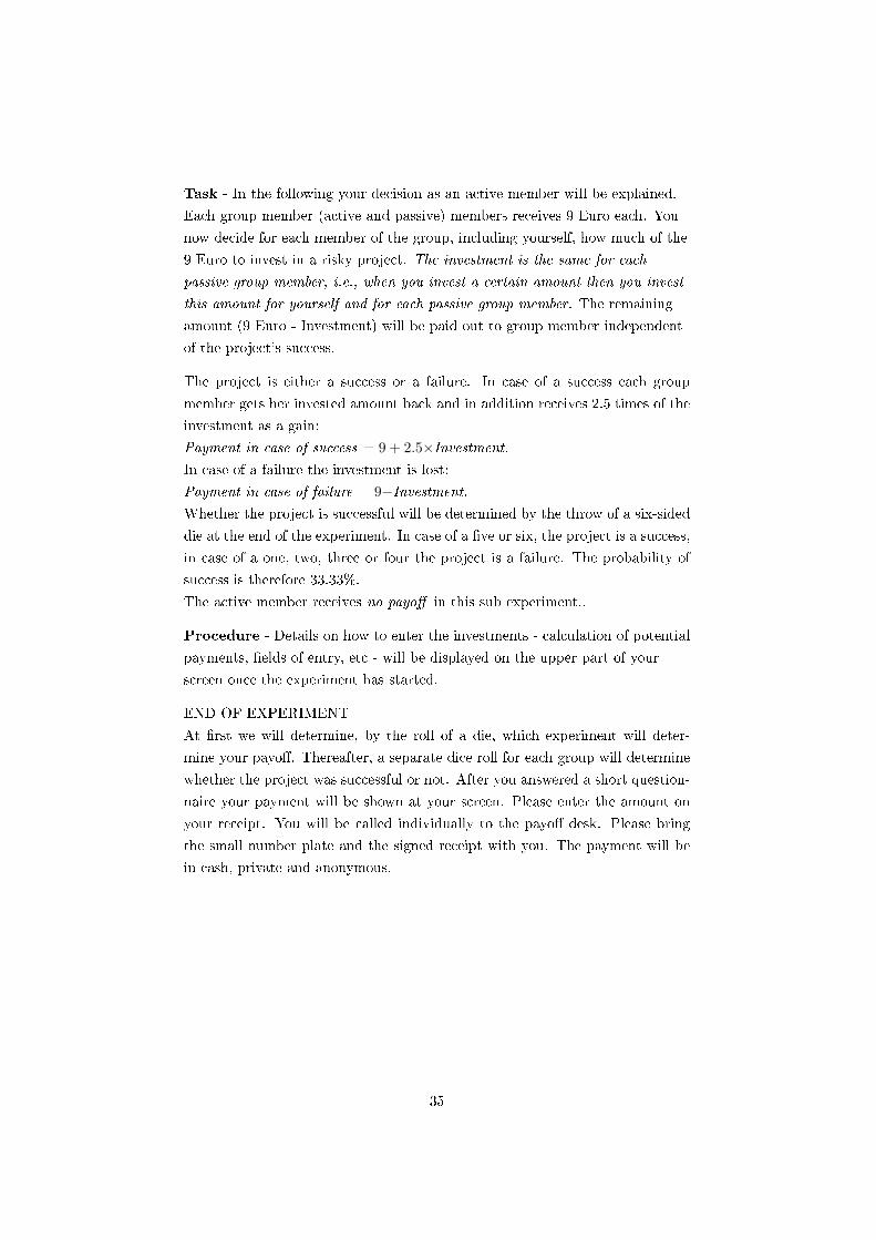
Task - In the following your decision as an active member will be explained.

Each group member (active and passive) members receives 9 Euro each. You

now decide for each member of the group, including yourself, how much of the

9 Euro to invest in a risky project. The investment is the same for each

passive group member, i.e., when you invest a certain amount then you invest

this amount for yourself and for each passive group member. The remaining

amount (9 Euro - Investment) will be paid out to group member independent

of the project's success.

The project is either a success or a failure. In case of a success each group

member gets her invested amount back and in addition receives 2.5 times of the

investment as a gain:

Payment in case of success = 9 + 2.5×Investment.

In case of a failure the investment is lost:

Payment in case of failure = 9−Investment.

Whether the project is successful will be determined by the throw of a six-sided

die at the end of the experiment. In case of a �ve or six, the project is a success,

in case of a one, two, three or four the project is a failure. The probability of

success is therefore 33.33%.

The active member receives no payo� in this sub experiment..

Procedure - Details on how to enter the investments - calculation of potential

payments, �elds of entry, etc - will be displayed on the upper part of your

screen once the experiment has started.

END OF EXPERIMENT

At �rst we will determine, by the roll of a die, which experiment will deter-

mine your payo�. Thereafter, a separate dice roll for each group will determine

whether the project was successful or not. After you answered a short question-

naire your payment will be shown at your screen. Please enter the amount on

your receipt. You will be called individually to the payo� desk. Please bring

the small number plate and the signed receipt with you. The payment will be

in cash, private and anonymous.

35

GLiterature

Overview

TableG.10:

Literature

Review

Article

Game

Design

Support

PotentialConfoundE�ects

OWNvs.

OTH

Reynoldset

al.(2009)

BP

WS

CS

Accountability,Recency

E�ecta

EriksenandKvaløy(2010)

GP

BS

CS

Chakravartyet

al.(2011)

MPL/FPA

WS

RS/RS

Polman(2012)

Invest

inCoin

Toss

WS

RS

Deception,Misaligned

Incentivesb

Anderssonet

al.(forthcoming)

MPL

BS

Nosigni�cante�ect

HighSocialDistance

MontinariandRancan(2013)

GP

WS

RS(friendsonly)

Accountability,Orderc

Pollmannet

al.(2014)

GP

BS

RS

OWNvs.

LEA

CharnessandJackson(2009)

Stag-HuntGame

BS

IndicationforCS

Sutter

(2009)

GPd

BS

RS

Implied

Accountability,Recency

E�ect

Pahlkeet

al.(2012)

BP

BS

CS

HumphreyandRenner

(2011)

MPL

BS

Nosigni�cante�ect

Accountability

Anderssonet

al.(forthcoming)

MPL

BS

Nosigni�cante�ect

HighSocialDistance

Boltonet

al.(2015)

MPL

WS

CS

Notes:

Inthetable,only

resultsin

thegain

domain

are

considered.Weconsider

signi�cantlevelsof5percent.

Abbreviations:

BP=

binary

prospects,achoice

betweentwolotteries(oroneriskylotteryandaguaranteed

payment).MLP=

multipleprice

list

inlinewithHoltandLaury

(2002),FPA=

�rstprice

auction

againstthecomputer,GP=designsimilarto

(Gneezy

andPotters,1997).WS/BS=within

subject

design/betweensubject

design.Thestudies�ndsupportfor

either

acautiousshift(CS),i.e.,more

risk

inOWNthanin

OTH/LEA,orariskyshift(R

S),i.e.,less

risk

takingin

OWNthanin

OTH/LEA.

aResultsmightbebiased.First

clients

inferred

theidentity

oftheinvestm

entmanager

(accountability).

Second,investm

entmanager

decided

always�rstforhimself,received

feedback,anddecided

afterward

fortheothers.

bSee

theirimplementationonpage119.

cIn

contrast

toGPthey

apply

alotterywithexpectedvaluebelow

endow

ment.

Each

subject

wentthroughthreetimes

12decisionswithorder

OWN,OTH(strangers),OTH(friends).

dIn

PAY-COMM

oneofthreein

agroupdecided

forrepetitions1-3,thesecondfor4-6,andthethirdfor7-9.

36

More information about the working paper series is available at the website of the Institute for Management Research: www.ru.nl/imr

Contact details

Sascha FüllbrunnInstitute for Management ResearchP.O. Box 9108 6500 HK Nijmegen The NetherlandsTel: + 31 (0) 24 – 361 54 74E-mail: s.fullbrunn@fm.ru.nl