AMBIENT AIR CONCENTRATION MODELING

Types of Pollutant Sources• Point Sources e.g., stacks or vents• Area Sources e.g., landfills, ponds, storage piles• Volume Sources e.g., conveyors, structures with multiple vents

Factors Affecting Dispersion of pollutants in the Atmosphere

Source Characteristics• Emission rate of pollutant• Stack height• Exit velocity of the gas• Exit temperature of the gas• Stack diameter

Meteorological Conditions• Wind velocity• Wind direction• Ambient temperature• Atmospheric stability

GAUSSIAN MODELS

Advantages• Produce results that match closely with experimental

data • Incorporate turbulence in an ad-hoc manner• Simple in their mathematics• Quicker than numerical models• Do not require super computers

Disadvantages• Not suitable if the pollutant is reactive in nature• Fails to incorporate turbulence in comprehensive

sense• Unable to predict concentrations beyond radius of

approximately 20 Km• For greater distances, wind variations, mixing

depths and temporal variations become predominant

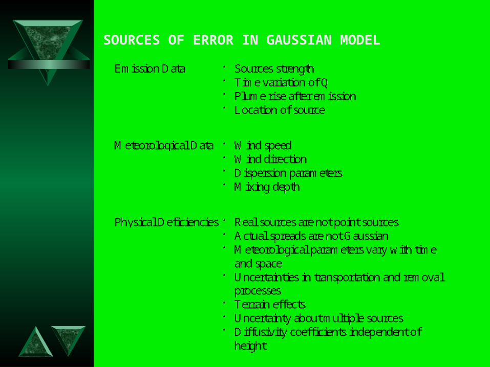
SOURCES OF ERROR IN GAUSSIAN MODEL

NUMERICAL SOLUTIONS

• Involves solving a system of partial differential equations• Equations mathematically represent the fate of pollutants

downwind concentration• The number of unknown parameters must be equal to

number of equations• System of equation is written in numerical form with

appropriate numerical scheme and solved using computer codes

Classes of Numerical Models

• Three Dimensional Equations (k-Theory) Model• Higher Order Closure Models (k- Type)

Difference between Numerical Models and Gaussian Model

• The degree of completeness in the mathematical description of the atmospheric dispersion processes

• Type of releases i.e., stack, jet or area source are easy to handle manually

• The models are designed to handle, degree of completeness in the description of non-transport processes like chemical reactions

• Terrain feature complexities for which the model is designed

Sources of Error In Numerical Models Based on K-Theory

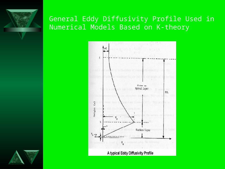
General Eddy Diffusivity Profile Used in Numerical Models Based on K-theory

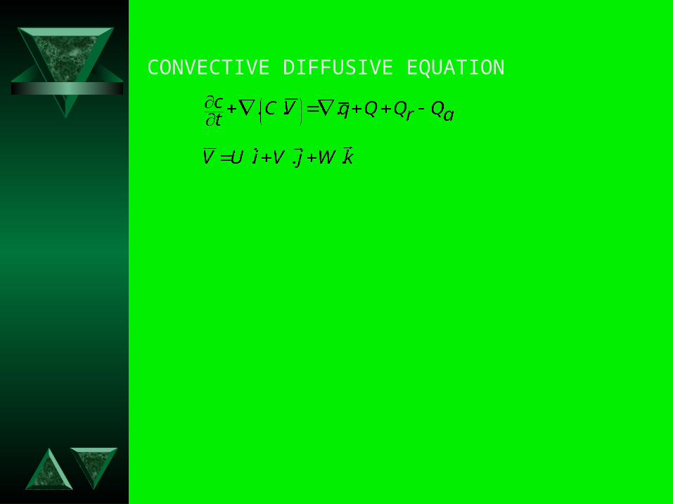
CONVECTIVE DIFFUSIVE EQUATION

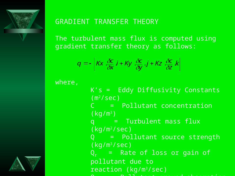
GRADIENT TRANSFER THEORY

The turbulent mass flux is computed using gradient transfer theory as follows:

where,K’s = Eddy Diffusivity Constants (m2/sec) C = Pollutant concentration (kg/m3) q = Turbulent mass flux (kg/m2/sec) Q = Pollutant source strength (kg/m3/sec) Qr = Rate of loss or gain of pollutant due to

reaction (kg/m3/sec) Qa = Pollutant ground absorption rate (kg/m3/sec) t = Time (sec) V = Wind field (m/sec)

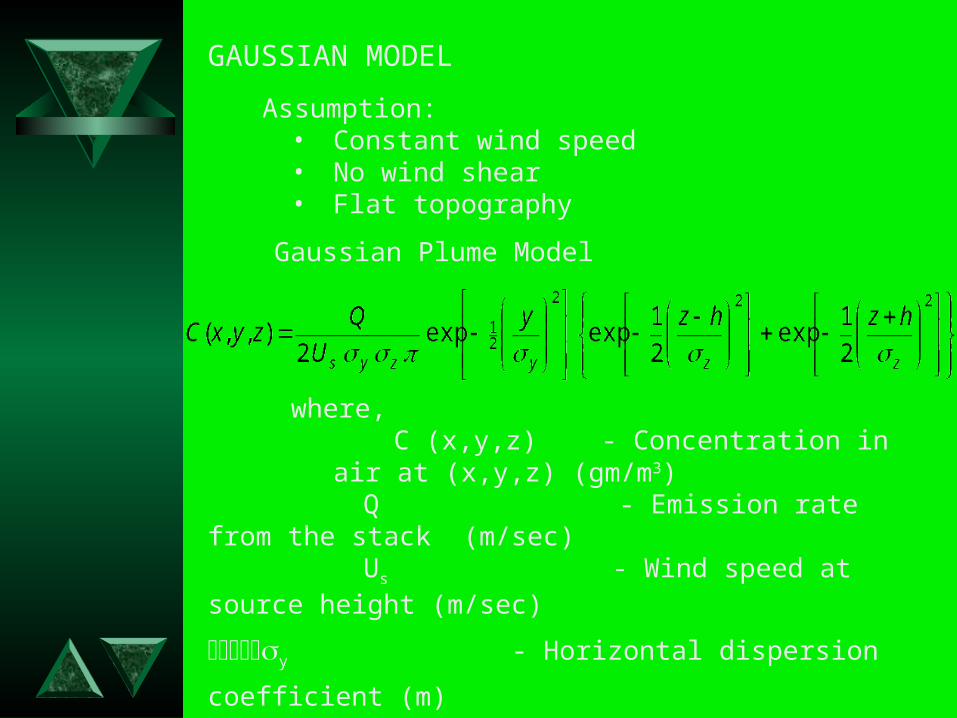
GAUSSIAN MODEL

Assumption:• Constant wind speed• No wind shear• Flat topography

Gaussian Plume Model

where,C (x,y,z) - Concentration in air at (x,y,z)

(gm/m3) Q - Emission rate from the stack (m/sec) Us - Wind speed at source height (m/sec)

y - Horizontal dispersion coefficient (m)

z - Vertical dispersion coefficient (m) y - Cross - wind distance (m) z - Vertical distance (m) h - Effective stack height (m)

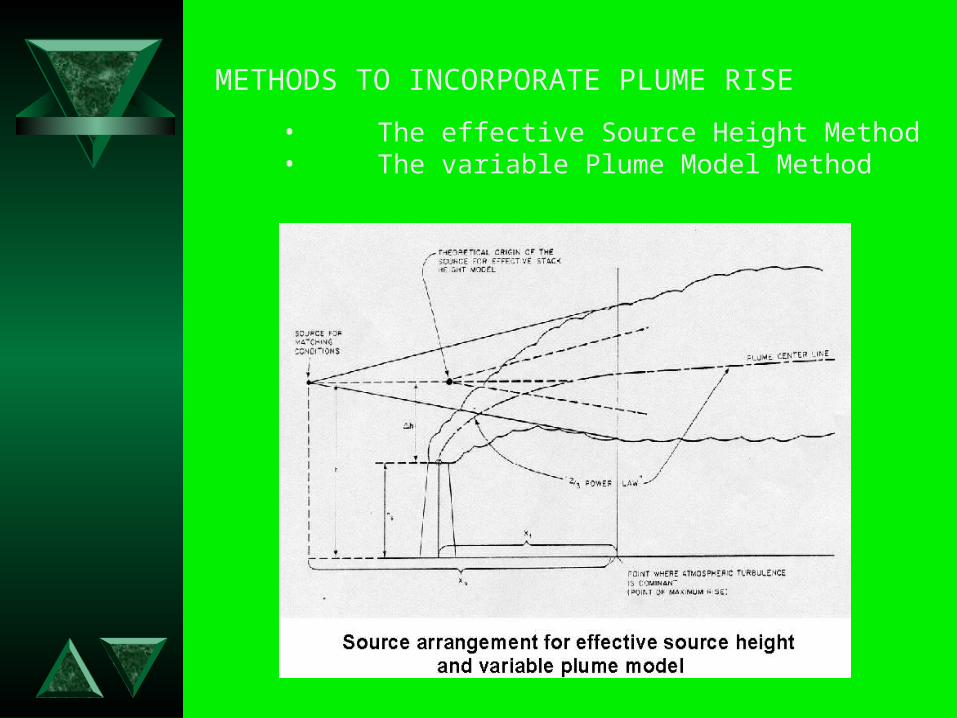
METHODS TO INCORPORATE PLUME RISE

• The effective Source Height Method• The variable Plume Model Method

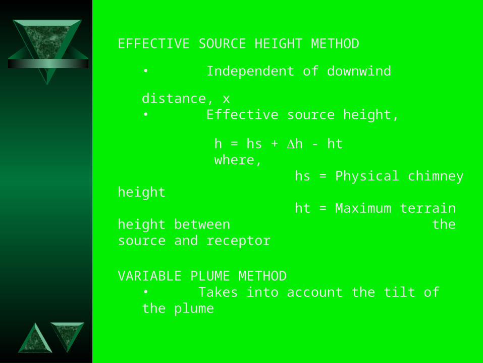
EFFECTIVE SOURCE HEIGHT METHOD

• Independent of downwind distance, x• Effective source height,

h = hs + h - htwhere, hs = Physical chimney height ht = Maximum terrain height between

the source and receptor

VARIABLE PLUME METHOD• Takes into account the tilt of the plume

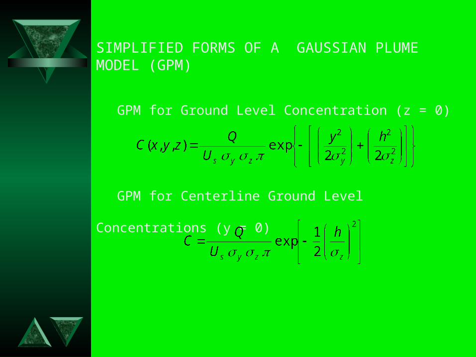
SIMPLIFIED FORMS OF A GAUSSIAN PLUME MODEL (GPM)

GPM for Ground Level Concentration (z = 0)

GPM for Centerline Ground Level Concentrations (y = 0)

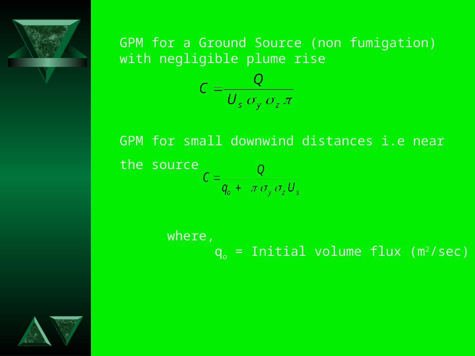
GPM for a Ground Source (non fumigation) with negligible plume rise

GPM for small downwind distances i.e near the source

where,qo = Initial volume flux (m2/sec)

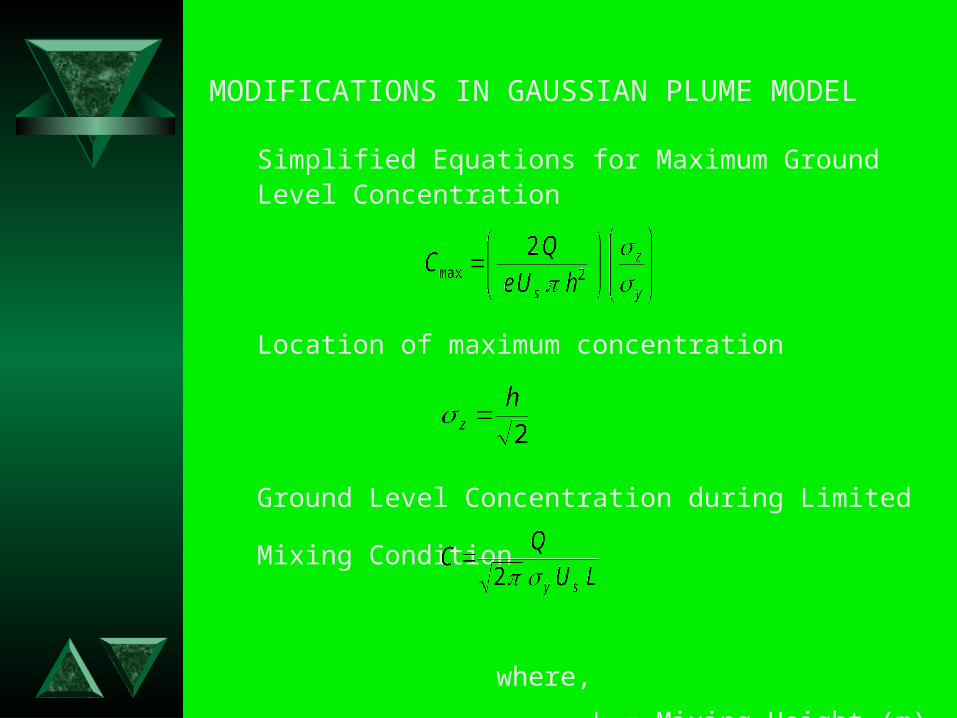
MODIFICATIONS IN GAUSSIAN PLUME MODEL

Simplified Equations for Maximum Ground Level Concentration

Location of maximum concentration

Ground Level Concentration during Limited Mixing Condition

where,

L = Mixing Height (m)

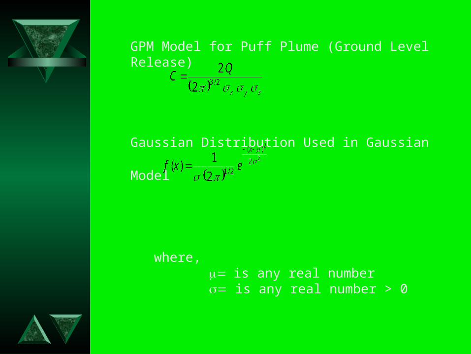
GPM Model for Puff Plume (Ground Level Release)

Gaussian Distribution Used in Gaussian Model

where, is any real number is any real number > 0

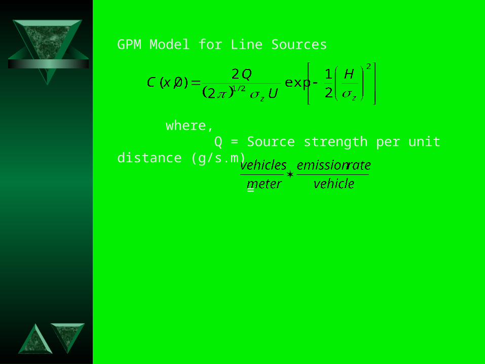
GPM Model for Line Sources

where,Q = Source strength per unit distance (g/s.m)

=

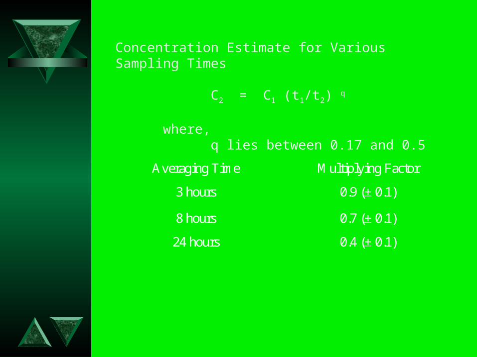
Concentration Estimate for Various Sampling Times

C2 = C1 (t1/t2) q

where,q lies between 0.17 and 0.5

Averaging Time Multiplying Factor

3 hours 0.9 (+ 0.1)

8 hours 0.7 (+ 0.1)

24 hours 0.4 (+ 0.1)

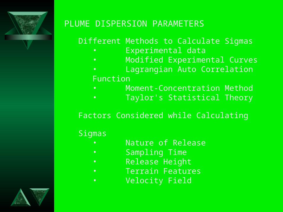
PLUME DISPERSION PARAMETERS

Different Methods to Calculate Sigmas• Experimental data• Modified Experimental Curves• Lagrangian Auto Correlation Function• Moment-Concentration Method • Taylor's Statistical Theory

Factors Considered while Calculating Sigmas• Nature of Release• Sampling Time• Release Height• Terrain Features• Velocity Field

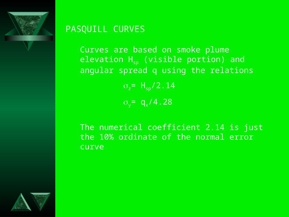
PASQUILL CURVES

Curves are based on smoke plume elevation Hsp (visible portion) and angular spread q using the relations

z= Hsp/2.14

y= qx/4.28

The numerical coefficient 2.14 is just the 10% ordinate of the normal error curve

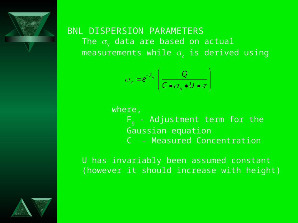
BNL DISPERSION PARAMETERS The y data are based on actual measurements while z is derived using

where, Fg - Adjustment term for the Gaussian equation C - Measured Concentration

U has invariably been assumed constant (however it should increase with height)

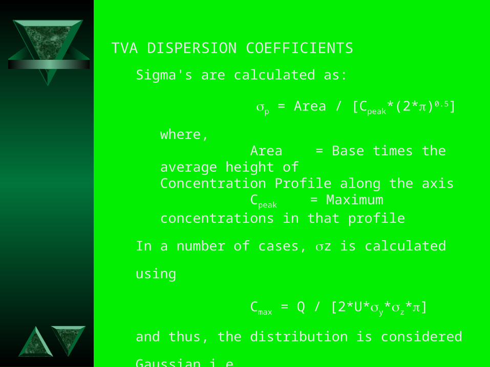
TVA DISPERSION COEFFICIENTS

Sigma's are calculated as:

p = Area / [Cpeak*(2*)0.5]

where, Area = Base times the average height of

Concentration Profile along the axis Cpeak = Maximum concentrations in that profile

In a number of cases, z is calculated using

Cmax = Q / [2*U*y*z*]

and thus, the distribution is considered Gaussian i.e.,

C = Cmax exp[-0.5*(xg/)2]

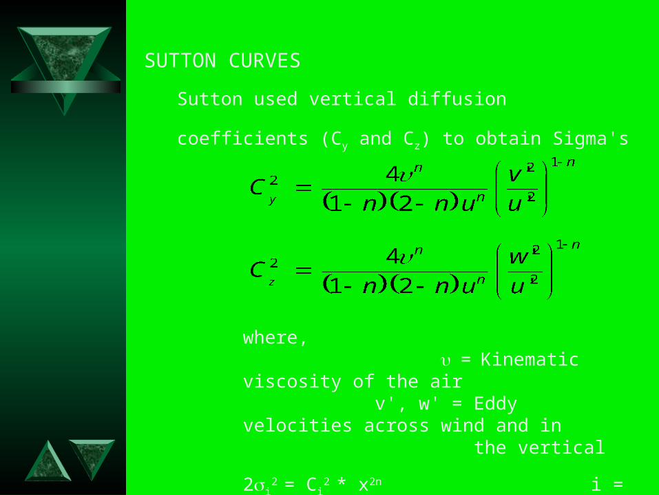
SUTTON CURVES

Sutton used vertical diffusion coefficients (Cy and Cz) to

obtain Sigma's

where, =Kinematic viscosity of the air v', w' = Eddy velocities across wind and in

the vertical

2i2 = Ci

2 * x2n i = y or z