american shad spawning migration …woofish.homestead.com/2007_final_shad_report.pdf · district of...

AMERICAN SHAD SPAWNING MIGRATION HYDROACOUSTIC MONITORING STUDY AT THE INTERSTATE 202 TOLL BRIDGE

ON THE DELAWARE RIVER AT LAMBERTVILLE, NEW JERSEY

17 MARCH to 31 MAY 2007

Submitted to:

THE DELAWARE RIVER BASIN FISH AND WILDLIFE MANAGEMENT COOPERATIVE

By:

BARNES-WILLIAMS ENVIRONMENTAL SERVICES d/b/a PACE ENVIRONMENTAL SERVICES

132 WASHINGTON STREET BINGHAMTON, NEW YORK 13901

(607) 723-3113

November 2007

2007 AMERICAN SHAD SPAWNING MIGRATION HYDROACOUSTIC MONITORING STUDY

PACE ENVIRONMENTAL SERVICES • 132 WASHINGTON STREET • BINGHAMTON, NEW YORK 13901 • (607) 723-3113 • Fax: (607) 723-8763 ii

TABLE OF CONTENTS

LIST OF TABLES AND FIGURES

1.0 INTRODUCTION...............................................................................................................1

2.0 EXECUTIVE SUMMARY ..................................................................................................2

3.0 METHODS AND MATERIALS ..........................................................................................3

3.1 SITE DESCRIPTION.....................................................................................................3

3.2 EQUIPMENT AND TRANSDUCER LOCATIONS.........................................................3

3.3 HYDROACOUSTIC SAMPLING PROTOCOL ..............................................................4

3.4 PRELIMINARY DATA AUDITING .................................................................................5

3.5 DATA HANDLING AND ANALYSIS ..............................................................................6

4.0 RESULTS..........................................................................................................................9

4.1 RIVER PARAMETERS..................................................................................................9

4.2 HYDROACOUSTIC FEASIBILITY ................................................................................9

4.3 HYDROACOUSTIC DATA COLLECTION ..................................................................10

4.4 ESTIMATED FISH PASSAGE ....................................................................................10

4.5 FISH SPATIAL DISTRIBUTION..................................................................................11

4.6 FISH TEMPORAL DISTRIBUTION.............................................................................11

4.7 SPECIES COMPOSITION OF TARGETS ..................................................................12

5.0 DISCUSSION/CONCLUSIONS.......................................................................................13

BIBLIOGRAPHY

TABLES

FIGURES

APPENDIX A - Hydroacoustic Sampling Details

APPENDIX B - Daily Span American Shad Passage Figures


PACE ENVIRONMENTAL SERVICES • 132 WASHINGTON STREET • BINGHAMTON, NEW YORK 13901 • (607) 723-3113 • Fax: (607) 723-8763 iii

LIST OF TABLES AND FIGURES

TABLES:

TABLE 1. MEAN WATER TEMPERATURE, RIVER DISCHARGE, AND WATER SURFACE ELEVATION

TABLE 2. DAILY AMERICAN SHAD PASSAGE ESTIMATES

TABLE 3. STUDY PERIOD SHAD PASSAGE ESTIMATES 17 MARCH TO 31 MAY 2007

TABLE 4. REVISED STUDY PERIOD SHAD PASSAGE ESTIMATES 17 MARCH TO 31 MAY 2007

FIGURES:

FIGURE 1. TRANSDUCER AND EQUIPMENT PLACEMENT LOCATIONS BRIDGE AND RIVER SECTION - VIEW LOOKING UPSTREAM

FIGURE 2. MEAN DAILY DISCHARGE AND WATER SURFACE ELEVATION

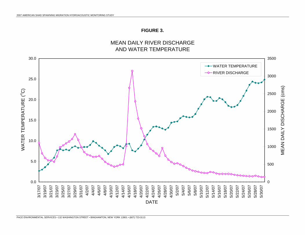
FIGURE 3. MEAN DAILY DISCHARGE AND WATER TEMPERATURE

FIGURE 4. SHAD PASSAGE DISTRIBUTION BETWEEN AND WITHIN SPANS

FIGURE 5. SHAD PASSAGE VERTICAL DISTRIBUTION

FIGURE 6. ESTIMATED DAILY SHAD PASSAGE - ALL SPANS

FIGURE 7. HOURLY SHAD PASSAGE DISTRIBUTION

FIGURE 8. MEAN DAILY RIVER DISCHARGE AND HISTORICAL FLOW DATA

FIGURE 9. ESTIMATED SHAD PASSAGE AND WEIGHTED MEAN UNIT SHAD DENSITY 1996 & 1998 TO 2007 MONITORING STUDIES


PACE ENVIRONMENTAL SERVICES • 132 WASHINGTON STREET • BINGHAMTON, NEW YORK 13901 • (607) 723-3113 • Fax: (607) 723-8763 1

1.0 INTRODUCTION

In March 2007, Barnes-Williams Environmental Services, LLC (BWES), d/b/a PACE Environmental Services (PACE), was authorized by the New Jersey Division of Fish and Wildlife (NJDFW) on behalf of the Delaware River Basin Fish and Wildlife Management Cooperative (Cooperative) to conduct a hydroacoustic study to assess the upstream spawning migration of adult American shad (Alosa sapidissima) in the Delaware River. The study involved the application of underwater sound transmitters/receivers (hydroacoustics) to monitor upstream American shad migration past the Interstate 202 Toll Bridge located on the Delaware River at Lambertville, New Jersey. The study was the fourteenth year of hydroacoustic studies at the toll bridge site and a continuation of the American shad spawning migration hydroacoustic monitoring conducted on the Delaware River at Lambertville in April of 1991 (BWEC 1991), April and May of 1992, 1995, 1996, 1998, 1999, and 2000 (BWEC 1992, 1995, 1996, 1998, 1999, 2000), and March, April, and May of 2001, 2002, 2003, 2004, 2005 and 2006 (PACE 2001, 2002, 2003, 2004, 2005, 2006).

The primary objective of this fisheries hydroacoustic study was to provide data addressing the timing and magnitude of the 2007 adult American shad population spring upstream spawning migration. The original hydroacoustic monitoring protocol included sampling in five of the wetted Interstate 202 Toll Bridge arch spans starting on 17 March (providing two weeks of March sampling) and continuing through 31 May 2007. The study was designed and the hydroacoustic data were collected to address the study objectives.

Information required to develop the shad passage estimates included daily river discharge data and daily water surface elevation data at the toll bridge site.1 The New Jersey District of the United States Geological Survey (USGS) at Trenton, NJ and the Delaware River Joint Toll Bridge Commission (DRJTBC) provided these data, respectively. Additionally, the New Jersey District of the USGS provided historic Delaware River discharge records for the 1913 to 2006 water years, and the Pennsylvania District of the USGS provided water temperature data for the Delaware River recorded below Tohickon Creek at Point Pleasant, PA.2

1 Water surface elevation data were recorded at the New Hope-Lambertville Toll-Supported Bridge (formally referred to as the “Free Bridge”) located approximately 1 mile (1.6 km) downstream from the Interstate 202 Toll Bridge. These data were used to predict gauge at the Route 202 Toll Bridge. 2 Point Pleasant, PA is located along the Delaware River approximately 7 miles (11 km) upstream of the Interstate 202 Toll Bridge.



2.0 EXECUTIVE SUMMARY

1. The sampling program for the 2007 American shad spawning migration hydroacoustic monitoring study began on 17 March and continued through 31 May 2007.3

2. Using the hydroacoustic technique of echo integration, American shad upstream migration in the Delaware River at Lambertville, New Jersey was assessed from piers of the Interstate 202 Toll Bridge; five wetted spans were monitored at the selected study site.

3. It was assumed that American shad schools could be visually distinguished (target classification) from other large fish targets by the characteristics of their echo pattern.4

4. Total American shad migration past the Toll Bridge was estimated by assuming that shad size and consequent individual fish echo intensity was uniform, and shad school swimming speed past the monitoring location was constant at 1.0 m/sec.

5. For the periods monitored,5 estimated shad passage was highest (over 2,000 fish) on the following days: 11 and 29 April; and 2-15, 17, 19, 22, 23, and 25 May 2007. It was estimated that approximately 65% of the 2007 upstream American shad run passed the toll bridge during these twenty-one days.6

6. Estimated shad passage was greatest in wetted bridge Span 4. It was estimated that approximately 78% of the 2007 shad run passed the toll bridge using this span.7

7. Shad passage was highest (99% of estimated total) in the daylight hours between 5:00 am and 7:00 pm (Eastern Standard Time), with a minor peak occurring at 6:00 pm. Estimated shad passage was low during darkness periods with little evidence of fish milling at night.

8. Delaware River discharge was at or above average (relative to historical flow data) from 17 March to 2 April. From 3 April to 14 April river discharge was below the mean historical discharge for those dates. On 15 April discharge began to increase to above average levels again, peaking at over 3,100 cms (≈110,000 cfs) on 17 April, and it remained above average through 4 May. River discharge was declining and generally continued to declined from 5 May on, remaining below average over the next three weeks through the end of the study.

9. Total American shad passage at Lambertville during the 76-day monitoring period was estimated to be 181,600±1,600 fish (95% Confidence Interval).8 This estimate is indicative of an increase in the magnitude of the adult 2007 American shad spawning-run compared to the 2006 population estimate.

10. If it is assumed that there was no shad passage during 27-30 March and 16-21 April, when no reliable data were collected in any of the spans and when river discharge was extremely high (>1,100 cms; or 40,000 cfs), then total shad passage at Lambertville would be estimated to be 155,900±1,400 fish (95% CI). This shad passage estimate is still indicative of an increase in the magnitude of the adult 2007 American shad spawning-run compared to 2006, but is more conservative on the side of the fisheries resource.

3 In 2007 there were delays with the processing and approval of the shad hydroacoustic-monitoring contract. Sampling in all 5 wetted Route 202 Toll Bridge spans did not start until 3 April 2007. 4 It was assumed that American shad schools could be visually distinguished from Gizzard shad (Dorosoma cepedianum) and other resident fish species/schools based on their observed, distinct hydroacoustic echo pattern, school size, and unique behavioral characteristics. 5 In 2007 there were a number of days on which less than 24 hours of hydroacoustic data were collected in some, or all, of the toll bridge spans due to high river flows or equipment power supply problems. 6 Analysis was based on daily shad passage estimates for each span (Table 2). 7 Analysis was based on study period shad passage estimates for each span (Tables 3 and 4). 8 Estimate confidence limits do not take into account other possible (and likely) sources of variability; see assumptions detailed in Section 3.5, Data Handling and Analysis.



3.0 METHODS AND MATERIALS

3.1 SITE DESCRIPTION In 1991, the Interstate 202 Toll Bridge, located approximately 18 km upstream from Trenton, NJ, was pre-selected by the NJDFW to monitor American shad passage on the Delaware River. Maintained by the DRJTBC, the bridge crosses the Delaware River between Lambertville, NJ and New Hope, PA. At normal water surface elevation (49.0 ft or 14.9 m), the river at the bridge is approximately 270 meters wide and has a wetted cross-sectional area of approximately 440 m2. At this elevation the bridge piers divide the river into 6 separate channels (Figure 1).

The toll bridge site was initially selected for hydroacoustic monitoring because: it is downstream of the American shad spawning grounds on the Delaware River; the tops of the bridge piers are accessible via a catwalk that runs beneath the bridge and they provide protected locations for the hydroacoustic sampling gear; and the piers divide the river into discrete, separate channels. The bridge structure is conducive to the use of hydroacoustics to monitor fish passage on the river because in most areas the river is too wide and shallow to monitor using hydroacoustics. Also, each of the separate wetted bridge spans can be isolated to determine the spatial distribution and behavior of the upstream migrating adult shad as they pass under the bridge.

As upstream-migrating American shad approach the Lambertville/New Hope area, they first encounter a wing dam located approximately 3,500 feet (1 km) south of the New Hope-Lambertville Toll-Supported (Free) Bridge, which funnels them toward the center of the river. From this wing dam the Delaware River thalweg runs NNW under Span 2 (second span in from the western [PA] shore) of the Free Bridge (Casper 2005), crossing over to the eastern (NJ) side of the river along the mouth of Alexauken Creek, and then passing under wetted Span 4 of the Route 202 Toll Bridge (Figure 1). North of the toll bridge the line of maximum river depth crosses back over to the western side of the river again (Yates 2006).

3.2 EQUIPMENT AND TRANSDUCER LOCATIONS Transducer sampling and equipment placement locations at the Interstate 202 Toll Bridge were identified and established in 1991 (BWEC, 1991). These sampling sites were used in the 1991-1992, 1995-1996, 1998-2006 studies, and again in the 2007 monitoring program (Figure 1).

Taking advantage of low Delaware River flows, transducers and equipment installation began on 14 March 2007. At this time one 3.0° half-power beamwidth transducer was mounted in wetted Span 1, and all the other transducers were connected (to the pier-top equipment) and pulled to the top of the piers to protect them from damage from predicted high river discharge. After delays with processing and approval of the 2007 hydroacoustic monitoring contract were resolved (see Appendix A), and as soon as Delaware River flows declined to safe working conditions again, transducers were installed and positioned in wetted Spans 2-5, the sampling equipment was calibrated (final site calibrations), and data collection started in all 5 bridge spans on 3 April 2007.

In wetted Span 1, one (1) transducer was mounted to the pier 2.5 feet above the river bottom (Figure 1). In wetted Spans 2, 3, 4, and 5, two transducers were mounted 2 feet apart on a length of steel pipe and suspended in fixed locations with the transducers 2.5 ft. and 4.5 ft. above the bottom (Figure 1). The transducers were positioned to maintain good sampling coverage along the bottom of their respective spans (BWEC 1992). Span 6 was not sampled due to its shallow depth and small cross-sectional area.

The face of each transducer was oriented horizontally toward the opposite pier (toward the river bank in the case of wetted Span 1). Prior to transducer placement, the hydroacoustic



equipment was hoisted to the tops of the piers, assembled, and installed in protective storage lockers, which were affixed to the pier-access catwalk ladders. The following is a list of equipment installed at the Interstate 202 Toll Bridge at Lambertville in 2007.

• Nine (9), 3° half-power beamwidth, 200 kHz transducers

• Three (3), 200 kHz signal processors with appropriate interface for IBM-compatible computers (transmitters/receivers)

• Three (3), IBM-compatible computers, each with a hard disk capable of storing the entire two (plus) month data set

• Three (3) Transducer switching devices (TSD’s) with appropriate ports to interface between the signal processors and the computers

• Site-specific, proprietary hydroacoustics sampling software

Due to the shallow river depths between bridge piers, narrow beamwidth transducers were necessarily used to horizontally sample the entire linear distance between piers (BWEC 1991). The distance ranges sampled by each transducer in each wetted bridge span are presented in Appendix A, Table A-1. Three distance ranges were sampled in wetted Spans 2-5. In Span 1 only one range (the range closest to the pier) was sampled, since under normal water surface elevation conditions only a portion of the span is wetted.

As previously described, on 3 April 2007 the transmitter/receiver signal processors were site calibrated (Appendix A) and normalized to each other such that the echo received from a given target at a specified range would be the same for the three pieces of sampling gear. Instrument controls and fish detection threshold levels were set to be as sensitive as the background acoustic noise would permit. Once calibrated, the equipment was tested for several hours to evaluate the operating condition of the hardware and software.9 Final instrument control adjustments were made and data collection at the Interstate 202 Toll Bridge at Lambertville for all equipment setups (sampling in Span 1 had actually begun on March 17) commenced on 3 April 2007. The first full day of sampling in all 5 wetted bridge spans was 4 April.10 The hydroacoustic sampling equipment was removed from the site on 4 June 2007.

3.3 HYDROACOUSTIC SAMPLING PROTOCOL Echo pulse signals were generated and received by each transmitter/receiver through one of the site transducers (user-selected sequencing controlled by the computer software). Transducer sampling was conducted systematically. Wetted Span 1 was sampled continuously using the one transducer installed in the span (until 24 April when the transducer had to be moved to Span 2 – see Appendix A). In the deeper spans (2, 3, 4, and 5), at the equipment setups used to sample two spans, one span was sampled for one minute, and then the other span was sampled for the next minute, switching between the upper and lower transducers in a given span (except for Span 2 where one transducer [bottom] was sampled from 24 April on). Thus, sampling was conducted in each span for approximately 50% of the time, while each transducer in the span was sampled 25% of the time.

The transmitted signals were generated at a maximum rate of one (1) pulse per second (user defined time interval). This pulse rate was selected to maintain non-overlapping sample 9 All sampling equipment components were also extensively tested and calibrated prior to site deployment. 10 A detailed description of days and hours sampled and of the different problems encountered during sampling is provided in Appendix A.



volumes between each transmitted and received echo pulse. The received analog echo signals were processed and digitized by the transmitter/receiver. Each digitized echo pulse signal (transmitter/receiver video image) was copied to the computer memory and redisplayed on the computer monitor as the primary Quality Control check to insure proper data transfer.

Each echo pulse, received at a rate of approximately one (1) pulse per second, was examined for targets by the monitoring computers. The examination occurred over user-selected range intervals for each transducer (Appendix A, Table A-1). If the echo level measured within a given range interval exceeded the preset noise threshold level (Section 3.2), that sample was tagged as containing detected targets for later review.

After a user-selected period (in this case, one minute), a summary of all the targets detected during the preceding 60 seconds was processed and saved to a data file. The target summaries included information on the transducer at which the targets were detected, the number of echo pulses included in each summary, the minute of the day over which the data were summarized, and the echo strength of the detected targets. At the end of each one-minute sample period, a different transducer was then sampled, such that all of the transducers at each equipment setup were sequentially sampled. At the end of each hour, the files containing the saved transmitter/receiver images were compressed and saved to the computer’s hard drive. At the end of the day (midnight) the data summary file was also compressed, and it and the last hourly image files were saved to the computer’s hard drive.

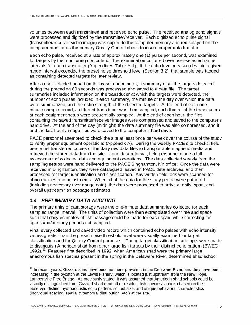
PACE personnel attempted to check the site at least once per week over the course of the study to verify proper equipment operations (Appendix A). During the weekly PACE site checks, field personnel transferred copies of the daily raw data files to transportable magnetic media and retrieved the stored data from the site. Upon data retrieval, field personnel made a full assessment of collected data and equipment operations. The data collected weekly from the sampling setups were hand delivered to the PACE Binghamton, NY office. Once the data were received in Binghamton, they were catalogued, saved in PACE data archives, and then processed for target identification and classification. Any written field logs were scanned for abnormalities and adjustments. When all of the data for the study period were gathered (including necessary river gauge data), the data were processed to arrive at daily, span, and overall upstream fish passage estimates.

3.4 PRELIMINARY DATA AUDITING The primary units of data storage were the one-minute data summaries collected for each sampled range interval. The units of collection were then extrapolated over time and space such that daily estimates of fish passage could be made for each span, while correcting for spans and/or study periods not sampled.

First, every collected and saved video record which contained echo pulses with echo intensity values greater than the preset noise threshold level were visually examined for target classification and for Quality Control purposes. During target classification, attempts were made to distinguish American shad from other large fish targets by their distinct echo pattern (BWEC 1992).11 Features first described in 1992, when American shad were the primary large, anadromous fish species present in the spring in the Delaware River, determined shad school

11 In recent years, Gizzard shad have become more prevalent in the Delaware River, and they have been increasing in the bycatch at the Lewis Fishery, which is located just upstream from the New Hope/ Lambertville Free Bridge. As previously stated, it was assumed that American shad schools could be visually distinguished from Gizzard shad (and other resident fish species/schools) based on their observed distinct hydroacoustic echo pattern, school size, and unique behavioral characteristics (individual spacing, spatial & temporal distribution, etc.) at the site.



identification criteria. Consequently, shad school classification has become subjectively standardized, based on years of experience of target recognition at the site. Shad school classification was also conservative on the side of the fish resource, as questionable identification samples were not tagged as shad schools.

Because the background noise levels were both elevated and episodic, a mean echo intensity value for the background noise in each one-minute sample containing classified shad targets was computed by evaluating one-minute samples before and after those with classified targets. The mean integrated sound intensity of the background noise was subtracted from that of the one-minute sample containing classified shad targets to calculate echo intensity values for the shad schools alone. After target classification and noise filtration, the one-minute integrated echo intensity value sums for each transducer range (cell) were divided by the average individual American shad echo intensity value (BWEC 1992)12 to calculate shad passage sums per cell per minute. Shad densities for each transducer range were then estimated and these cell shad densities were used to estimate span and total shad passage during the study.

3.5 DATA HANDLING AND ANALYSIS Transducer sampling volumes were estimated as in previous monitoring years. The ensonified zones for the two ranges closest to the transducers were treated as truncated 2° cones with the apex of the cone at the transducer face and the cone axis the same as the transducer beam axis. Sample volume of these truncated cones was calculated using the following formula:

vol. = (π/3) * tan2(1°) * (Rangemax3 - Rangemin

3) = 3.1906E-4 * (Rangemax

3 - Rangemin3).

The ranges farthest from the transducers were treated as cylinders with volumes as follows:

vol. = π * (tan(1°) * Rangemin)2 * (Rangemax - Rangemin).

The estimated volumes sampled per pulse by each transducer and each range are presented in Appendix A, Table A-1.

In order to compensate for the different sampled volumes of the various transducers and ranges (cells), the numbers of shad estimated per one-minute sample per transducer per range interval were weighted by converting to a shad density estimate (fish/m3 per one-minute sample per transducer range) using the following formula:

Fish DensityCELL = Estimated Fish DetectedCELL PVCELL * PulsesCELL

where: Fish = One-minute Echo Value Sum / Individual Shad Echo Value PV = Sampled Volume per echo pulse (m3) Pulses = Number of echo pulses examined per one-minute sample Cell = A transducer range interval.

12 In 1992, mean American shad individual “acoustic size” was estimated using echo intensity data collected from a standard target, from live, lateral-aspect-tethered shad targets, and from individual, hydroacoustic fish targets (also assumed to be in lateral aspect to the transducers) that could be discriminated at the perimeter of large shad schools passing in the toll bridge spans.



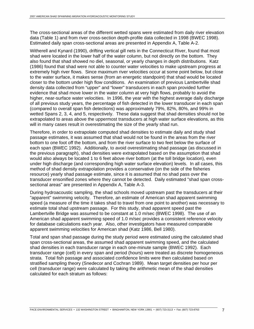
The cross-sectional areas of the different wetted spans were estimated from daily river elevation data (Table 1) and from river cross-section depth-profile data collected in 1998 (BWEC 1998). Estimated daily span cross-sectional areas are presented in Appendix A, Table A-2.

Witherell and Kynard (1990), drifting vertical gill nets in the Connecticut River, found that most shad were located in the lower half of the water column, but not directly on the bottom. They also found that shad showed no diel, seasonal, or yearly changes in depth distributions. Katz (1986) found that shad were not able to counter water velocities to make upstream progress at extremely high river flows. Since maximum river velocities occur at some point below, but close to the water surface, it makes sense (from an energetic standpoint) that shad would be located closer to the bottom under high flow conditions. An examination of previous Lambertville shad density data collected from “upper” and “lower” transducers in each span provided further evidence that shad move lower in the water column at very high flows, probably to avoid the higher, near-surface water velocities. In 1996, the year with the highest average daily discharge of all previous study years, the percentage of fish detected in the lower transducer in each span (compared to overall span fish detections) was approximately 79%, 82%, 80%, and 99% in wetted Spans 2, 3, 4, and 5, respectively. These data suggest that shad densities should not be extrapolated to areas above the uppermost transducers at high water surface elevations, as this will in many cases result in overestimating the size of the yearly shad run.

Therefore, in order to extrapolate computed shad densities to estimate daily and study shad passage estimates, it was assumed that shad would not be found in the areas from the river bottom to one foot off the bottom, and from the river surface to two feet below the surface of each span (BWEC 1992). Additionally, to avoid overestimating shad passage (as discussed in the previous paragraph), shad densities were extrapolated based on the assumption that shad would also always be located 1 to 6 feet above river bottom (at the toll bridge location), even under high discharge (and corresponding high water surface elevation) levels. In all cases, this method of shad density extrapolation provides a conservative (on the side of the fisheries resource) yearly shad passage estimate, since it is assumed that no shad pass over the transducer ensonified zones where they cannot be detected. Daily estimated "shad span cross-sectional areas" are presented in Appendix A, Table A-3.

During hydroacoustic sampling, the shad schools moved upstream past the transducers at their "apparent" swimming velocity. Therefore, an estimate of American shad apparent swimming speed (a measure of the time it takes shad to travel from one point to another) was necessary to estimate total shad upstream passage. For this study, shad apparent speed past the Lambertville Bridge was assumed to be constant at 1.0 m/sec (BWEC 1998). The use of an American shad apparent swimming speed of 1.0 m/sec provides a consistent reference velocity for database calculations each year. Also, other investigators have measured comparable apparent swimming velocities for American shad (Katz 1986, Bell 1980).

Total and span shad passage during the study period were estimated using the calculated shad span cross-sectional areas, the assumed shad apparent swimming speed, and the calculated shad densities in each transducer range in each one-minute sample (BWEC 1992). Each transducer range (cell) in every span and period (hours) were treated as discrete homogeneous strata. Total fish passage and associated confidence limits were then calculated based on stratified sampling theory (Snedecor and Cochran 1989). Mean target densities per hour per cell (transducer range) were calculated by taking the arithmetic mean of the shad densities calculated for each stratum as follows:



n

MFDCELL,HOUR = Σ Fish DensityCELL,MIN i=1_________________________ , nCELL,MIN

where n = the number of one-minute samples collected per hour per cell.

Shad density variance for each stratum (Cell, Hour) was calculated as follows: n

VFDCELL,HOUR = Σ (Fish DensityCELL,MIN - MFDCELL,HOUR)2 i=1______________________________________________ .

nCELL,MIN - 1

A weighted mean unit density (WMUD) was then calculated by taking the sum of the mean target densities per stratum multiplied by the corresponding stratum weight as follows:

n

WMUD = Σ (MFDCELL,HOUR * WeightCELL,HOUR) i=1

where Weighting Factor = Stratum Volume Sampled / Total Volume SampledALL STRATA.

This stratification is described as stratification with proportional allocation and gives a self-weighting sample (Snedecor and Cochran 1989).

When daily span shad passage was estimated, stratification was by cell and by hour of the day. When total study shad passage was estimated, stratification was by all transducer ranges for all spans, and by all hours of the study period. Total shad passage was calculated as follows:

Fish Passage = WMUD * Shad Cross Section Area * Shad Velocity * Time (fish/m3) (m2) (m/sec) (sec)

= WMUD * N (population units).

Variance of Unit Density (VUD) was calculated as follows:

n

VUD = Σ (WeightCELL,HOUR 2 * VFDCELL,HOUR) i=1___________________________________________

nCELL,HOUR

where n = number of strata in the daily or overall estimates.

The variance of unit density (VUD) was used to construct 95% confidence limits for weighted mean unit density (Snedecor and Cochran 1989). Confidence limits were calculated as follows:

95% CIWMUD = WMUD ± (1.96 * √VUD)

95% CIFISH PASSAGE = Fish Passage ± (1.96 * N * √VUD)

where N = population units as previously defined.



4.0 RESULTS

4.1 RIVER PARAMETERS Mean river discharge (as measured downstream at Trenton, New Jersey) was variable over the course of the study (Table 1, Figure 2). On 3 April, the first day of sampling in all 5 wetted bridge spans, average daily river discharge was below 760 cms. Flows remained between 700-750 cms through 6 April, and then steadily declined to below 500 cms by 10 April, remaining below this level through 14 April. On 15 April average daily river discharge suddenly increased to over 1000 cms. River discharge continued to increase, peaking at over 3,100 cms (≈110,000 cfs) on 17 April, at which point it began to decrease again, and it continued to generally decrease through the end of the study period, reaching low levels (<200 cms) by 22 May. In summary, during the 2007 hydroacoustic monitoring study, average daily Delaware River flows ranged from a low of 143 cms (≈5,050 cfs) on 30 May, to the high of 3,147 cms (≈111,150 cfs), which was recorded by the USGS on 17 April 2007 (Table 1, Figure 2).

Water surface elevation data were recorded by DRJTBC personnel at the New Hope-Lambertville Toll-Supported (Free) Bridge located approximately 1 mile (1.6 km) downstream from the Interstate 202 Toll Bridge, whereas daily river discharge was measured downstream at Trenton, NJ. Daily river surface elevations measured at the Free Bridge and mean daily river discharge were closely correlated (Table 1, Figure 2); river discharge increases resulted in corresponding rises in water surface elevation. Average daily river surface elevation was lowest on 30-31 May (<15.0 m), and highest on 17 April (>18.0 m). Mean water surface elevation at the Free Bridge was at or higher than the normal (yearly) water surface elevation of 14.9 m (49.0 ft.) on all 76 days of the 2007 monitoring period.

As stated in Section 3.5, Free Bridge river surface elevation data were used to estimate the daily wetted cross-sectional areas of each of the five sampled spans. The higher the water surface elevation, the larger the span cross-sectional areas were for each span. Over the course of the 2007 monitoring period, Spans 3, 4, and 5 had the largest cross-sectional wetted areas, accounting for approximately 70% of the total span wetted areas combined.

Average daily Delaware River water temperatures, recorded at Point Pleasant, PA, were variable over the course of the study period, ranging from a low of 2.7°C recorded on 17 March, to a high of 24.9°C measured at the end of the study on 31 May (Table 1, Figure 3). As expected for this time of year, water temperatures generally increased over the study period. Water temperature increased to above 9°C by 4 April and remained at this level for the next 2 days when it began dropping, falling below 7°C on 9 April. After that the water temperature generally continued to climb (except for during the high flow period of 17-19 April), reaching 10°C by 21 April, 15°C by 3 May, and 20°C by 11 May. Water temperatures remained above 15°C from 3 May through the end of the study period. As previously stated, water temperatures generally increased over the study period, and although there were some minor exceptions to this pattern, there were no large drops in average daily water temperatures in 2007.

4.2 HYDROACOUSTIC FEASIBILITY In 1992, hydroacoustic sampling was shown to be effective at the toll bridge site using the 3° half-power beamwidth transducers. The narrow beam transducers made it possible to sample across the entire width of each span, and noise levels caused by water surface and river bottom backscatter in the far sampling ranges were reduced. The echo patterns of the large adult American shad schools moving upstream through the acoustic beam were very distinct. As described by Chittenden (1969), the schools were usually v-shaped at the leading upstream end. Also, the schools were almost always streams or ribbons of large fish aggregates 2-3



meters wide, located primarily in the middle of the bridge spans. These features, which were first identified in 1992 when American shad were the primary large, anadromous fish species present in the Delaware River (at this time of year) provided shad school identification criteria to allow data auditors to attempt to distinguish upstream migrating shad from other resident river fish or boat traffic, as well as from milling shad.

Over the many years of hydroacoustic monitoring at the site there has been no evidence that the areas under the bridge are holding areas where shad collect and mill during periods of darkness. These conditions were consistent in the 2007 study. The toll bridge site was initially selected for hydroacoustic monitoring because it is upstream of the tidal areas of the Delaware River, and the site is downstream of the traditional American shad spawning grounds on the Delaware. The hourly distribution of large fish aggregates indicates that there is very little fish activity under the toll bridge during darkness periods. Further, identified large fish aggregates have not shown much horizontal movement while passing under the bridge, maintaining their horizontal position within spans over time. Consequently, it was assumed that the large identified passing fish aggregates that met all the migrating shad classification criteria were upstream migrating shad positioned in lateral aspect to the transmitted echo pulses.

4.3 HYDROACOUSTIC DATA COLLECTION Data collection formally began in Span 1 on 14 March 2007. As previously described, sampling was delayed at the other setups due to holdups with the processing and approval of the 2007 hydroacoustic monitoring contract, as well as high river discharge conditions. Sampling began in all 5 spans on 3 April 2007. During the 2007 monitoring period there were numerous days on which less than 24 hours of data were collected in some, or all, of the Route 202 Toll Bridge spans. A detailed explanation for these gaps in data collection is provided in the Hydroacoustic Sampling Details found in Appendix A.

4.4 ESTIMATED FISH PASSAGE As stated in Section 3.5, all one-minute sample periods that contained echo pulses with echo values greater that the preset noise threshold were visually examined for target classification. One-minute summaries, which did not contain classified targets, and which occurred immediately before and immediately after those with classified targets, were used to estimate the ambient noise level in the samples with targets. After removing (subtracting) the noise from samples with these classified targets, the echo-intensity value of the classified shad schools was divided by the individual shad echo-intensity value to arrive at estimates of shad density in those one-minute samples.

Each transducer was sampled for only a portion of the time each day. Therefore, the one-minute span shad density estimates, calculated for each transducer and range, were used to calculate Weighted Mean Unit shad densities for each span, which in turn were multiplied by the daily estimated span shad extrapolation volumes to calculate total daily span shad passage (Section 3.5). These daily span shad passage estimates are presented in Table 2.

Weighted Mean Unit shad densities were calculated for the entire study for each span separately, and for all spans combined. These densities were applied to (multiplied by) estimated shad extrapolation volumes (Section 3.5) to arrive at span and study (all spans combined) shad passage estimates. Span and overall study shad passage estimates are presented in Table 3. Based on all the assumptions detailed in Section 3.5, it was estimated that a total of 181,600±1,600 American shad adults passed under the Interstate 202 Toll Bridge in 2007. It should be noted that there are numerous factors, which are assumed to be constants for the purposes of these analyses, that undoubtedly introduced some additional variability to the fish passage estimates; these variability factors are not accounted for in the span, and



yearly shad passage confidence intervals. But it also should be noted that the constants have been uniformly maintained throughout the years of study at Lambertville.

As in 2005, in 2007 BWES also calculated “revised” study period shad passage estimates for the monitoring period (Table 4). Previous hydroacoustic data collected at Lambertville have indicated that shad do not make upstream progress during periods of excessively high river flows, and consequently it may not make sense to extrapolated computed mean fish densities to high discharge days during which no hydroacoustic data have been collected. If weighted mean shad densities were not extrapolated to 27 to 30 March or to 16 to 21 April (when flows were still over 40,000 cfs), and based on the same assumptions detailed in Section 3.5, it was estimated that a total of 155,900±1,400 American shad adults passed under the Interstate 202 Toll Bridge in 2007. This revised estimate is more conservative on the side of the fisheries resource.

The calculation of the daily shad passage and the total study are based on different sample sizes. Therefore, although the estimates are similar in magnitude, some differences will occur. The daily passage estimates (Table 2) should be used to characterize the relative daily and span distribution of fish passing the site, whereas the entire study passage estimates (Tables 3 and 4) should provide the best estimates of the actual magnitude of the overall 2007 American shad migration.

4.5 FISH SPATIAL DISTRIBUTION Shad passage in Spans 1, 2, 3, 4, and 5 was estimated at approximately: 0; 11,700; 2,100; 129,800; and 22,400 fish, respectively (Table 4). From these data, the percentages of fish passing through each of Spans 1-5 were estimated at 0.0%, 7.0%, 1.3%, 78.2%, and 13.5%, respectively.

Data from days on which 4 spans (2-5) were sampled were used to examine shad horizontal distribution at the toll bridge, as in Span 1 no targets were identified (see Section 3.2) in 2007 monitoring. In Span 2, the majority of detected shad passed in the middle sampling range (Figure 4). In Span 3, most of the fish were detected in the sampling range on the east (NJ) side (Figure 4). In Span 4 fish were detected in the center range, while in Span 5 the majority of fish were identified in the western most (PA side) range (Figure 4).

Data from all spans were used to examine shad vertical distribution at the toll bridge. In Span 1 no fish were detected. In Spans 2, 4 and 5 most of the fish were detected by the lower transducer, while in Span 3 fish were primarily detected by the upper span transducer (Figure 5). It should be noted that there was some vertical overlap between the volumes sampled by the upper and lower transducers. It should also be noted that for a good portion of the study the upper transducer in Span 2 was not sampled due to low flow/water surface conditions and there was no upper transducer mounted in Span 2 after 24 April.

4.6 FISH TEMPORAL DISTRIBUTION As previously detailed, no data were collected in Spans 2-5 prior to April 3. No shad schools were detected in Span 1 prior to April 3, but this span typically has few shad detections, and there is no way to make any kind of inferences regarding shad passage in Spans 2-5 during this time period. During the 2007 study, shad (large fish aggregates meeting shad classification criteria) were detected in Span 4 on 5 April, soon after all the equipment was installed at the site (Table 2, Figure 6). No large fish aggregates were detected after 27 May. As previously noted, there were a number of days on which less than 24 hours of hydroacoustic data were collected in some, or all, of the bridge spans. But these gaps in data collection were associated with river conditions that would prohibit fish passage, so this is probably not a major concern when discussing study results related to the seasonal distribution of American shad at Lambertville in



2007. From 29 April through 27 May shad passage was consistent, with small schools passing the 202 Toll Bridge site almost every day. In 2007, Span 4 was apparently the main avenue of upstream shad passage; there were 25 days with over 1000 fish, and 6 days with over 5,000 fish estimated in the span (Table 2). These six days of highest fish passage in Span 4 occurred between 3 May and 13 May. Estimated American shad passage, by span, is depicted in Appendix B, Figures B-1 to B-4.

The diel distribution of fish passage was examined for all spans using data from all the days that were fully sampled (Figure 7). The hours with the lowest number of samples with detected targets, and consequently the lowest estimated fish passage, were hours 0-4, and hours 19-24.13 Estimated shad passage was highest (99% of estimated total) in the daylight hours between 5:00 am and 7:00 pm, with a small early evening peak at 6:00 pm.

4.7 SPECIES COMPOSITION OF TARGETS As previously stated in Section 4.2, in 1992 when American shad were the primary large, anadromous fish species present in the Delaware River, it was noted that the echo pattern of adult American shad schools moving through the acoustic beam was very distinct. In the visual records tagged as representative of shad schools, the fish aggregates were almost always continuous 2-3 meter wide streams of tightly packed individuals, which were located primarily in the middle of the deeper bridge spans. As previously stated, for this study it was assumed that upstream migrating American shad schools could be visually distinguished from Gizzard shad and other resident fish species/schools, as well as milling adult shad, based on their observed distinct hydroacoustic echo pattern, school size, and unique behavioral characteristics (individual spacing, spatial & temporal distribution, etc.) at the toll bridge sampling location.

The hydroacoustic data collected to date at Lambertville appear to support the assumption that the existing shad school classification criteria used each year are valid in separating migratory shad targets from resident fish. The seasonal and diel abundance patterns that have been discerned each year, as well as obvious correlations of estimated shad abundance with environmental variables such as water temperature and river discharge appear to be indicative of the detection of large, schooling, migratory fish species. If large fish species other than American shad are passing the Route 202 Toll Bridge at mid-channel in large numbers during the months of April and May each year, relative American shad abundance would be overestimated. It has been recommended that a study be undertaken to identify fish species composition at the toll bridge monitoring location and to determine cross-sectional habitat use of various fish species at the site. Until these correlative data have been collected, it is assumed that American shad are the primary large migratory species identified during hydroacoustic monitoring at Lambertville each year.

13 All computer times recorded in Eastern Standard Time; clocks were not changed to daylight savings time.



5.0 DISCUSSION/CONCLUSIONS

Historically, the American shad upstream spawning migration has always occurred in the months of April and May, and the timing of the yearly run has been very consistent for a century or more (Chittenden 1969). The timing of the 2007 Delaware River American shad migration appeared to follow this general pattern, and although no hydroacoustic data were collected in Spans 2-5 during March 2007, the shape of the population bell curve indicates that it is likely that the majority of the 2007 run occurred in the months of April and May. This year was the seventh year in which hydroacoustic sampling at Lambertville was initiated in the month of March, and in the previous six (2001, 2002, 2003, 2004, 2005, and 2006) monitoring years, some shad (large fish targets meeting shad classification criteria) were detected prior to April. In 2001, 2002, 2003, 2004, 2005 and 2006 monitoring, it was estimated that 14%, 9%, 5%, 14%, 0.5 % and 5% of the yearly adult American shad spawning-run occurred in the month of March, respectively. As in 2005, when water temperatures remained low throughout the month of March, water temperatures in 2007 stayed below 10°C, reaching a high of only 8.4°C by 31 March. Consequently, it appears unlikely that any larger numbers of American shad passed under the Route 202 Toll Bridge prior to April 2007.

Studies have demonstrated that hatching and survival of shad are at a maximum when water temperatures are between 15.5°C and 26.5°C, and the temperature-regulated migrations of shad bring individual populations to their home rivers at times when the river temperatures are approaching the level that is best for spawning (Leggett 1973). This appeared to be the case at Lambertville in 2007, as shad passage appeared to begin in earnest toward the end of April and continued through May, peaking on 5 May as water temperatures were increasing and approaching 15°C (Tables 1 and 2, Figures 3 and 6).

Several schools of shad moved upstream passed the Route 202 Toll Bridge in early April accounting for an estimated 13,000 fish. However, river discharge increased to over 1019 cms (≈36,000 cfs) on 15 April and remained high (mostly over 900 cms [≈32,000 cfs]) through the 27 April. Water temperatures were above 10°C after 21 April for the rest of the study, but high river discharges inhibited passage until 29 April. A few small schools were detected in Span 2. As the river discharge decreased, and accompanied by warming water temperatures, shad passage was consistent for the remainder of the study (Tables 1 and 2, Figure 6). Average water temperature was greater than 13°C from 29 April through the remainder of the study period. It was estimated that peak shad passage occurred in the period from 28 April to 27 May. As in past years, these data indicate that water temperature was an important factor in determining the timing of the upstream shad migration in the Delaware River in 2007.

A comparison of 2007 USGS Delaware River discharge readings with historic, 1913-2006 water year discharge records collected at Trenton, NJ indicated that river discharge was above average (average by day) when the monitoring program began in mid-March, remaining at or above average levels through the first week of April (Figure 8). Discharge was below average over the next week, through mid-April, and then quickly rose, remaining well above average through the end of April. River discharge peaked on 17 April, and the average daily discharge recorded on 16 April was actually the highest ever recorded for that date over 94 years of discharge records. At the end of April river discharge declined to average levels, and then, from the beginning of May on, discharge continued to decline and remained below average, reaching near-minimum levels in late May. As in previous years at Lambertville, detected shad passage pulses appeared to be correlated with daily river discharge levels.

The major shad passage events generally occurred at times of relatively low discharge when flows were waning following periods of elevated water levels. The best example of this in 2007



took place after the large discharge peak that began on 15 April, continuing through 28 April. Only the setup in Span 1 was operating, as the transducers in the other spans were lost or inoperable as a result of the high river discharge. Sampling equipment in Spans 2-5 was put back in operation on 25 April and no fish were detected until 28 April when river discharge had dropped to approximately 750 cms (≈26,500 cfs), and then only in Span 2, outside of the river thalweg. The next day, with river discharge at approximately 630 cms (≈22,000 cfs) and continuing to drop, over 4,000 shad targets were estimated passing upstream in Span 4. Span 4 was the primary shad aggregate detection route, with Span 5 next, for the remainder of the study (Table 3), as average daily river discharge continued to decline.

During their spawning migrations, American shad orient themselves to the main river channels, preferring the open areas and the deepest river sections (Leggett 1976). Shad appear to prefer certain water depths and velocities and adjust their swimming speed, depth, and location accordingly (Witherell and Kynard 1990, Dodson and Leggett 1973, 1974, Katz 1986). Span 4, accounting for 78% of the run, was the most consistently (in terms of total days) used bridge span over 2007 flow conditions, and as previously described, the main Delaware River thalweg runs under the toll bridge in this span. Span 2, which accommodated approximately 47% of the shad passage in 2006, provided for only approximately 7% of the run in 2007. Span 2 also had the highest estimated shad passage in 2005 monitoring. But in 1998, 1999, 2000, 2001, 2002, 2003, and 2004, the percentages of shad estimated using Span 2 (as percentages of overall yearly passage) were 1.7%, 5.6%, 13.0%, 18.7%, 6.9%, 6.1%, and 1.6%, respectively. In terms of horizontal shad passage distribution, the 2007 study results appear to be more in-line with the earlier monitoring years.

Although there has been some year-to-year variability, the overall diel pattern of fish detections at Lambertville in 2007 was similar to that previously reported for migrating American shad on the Delaware River. Shad school passage was greatest in the daylight hours, with morning, and late afternoon peaks. As in all previous years, very few large shad schools were detected in the Delaware River under the Interstate 202 Toll Bridge during darkness hours, and the bridge spans do no appear to be areas where shad consistently collect or exhibit milling behavior.

Overall estimates of American shad passage in 2007 are provided in Tables 3 and 4. Hydroacoustic sampling, from an equipment-sampling standpoint, was influenced by river discharge conditions. The initial installation of transducers in wetted Spans 2-5 was delayed because high water. After the monitoring contract processing and approval issue was resolved in late March, the installation of transducers in Spans 2-5 was again delayed due to high river flows. Once all equipment was installed at the beginning of April another high water event beginning on 15 April caused considerable damage and shut down data collection until 25 April. However river discharges were so high that the resulting loss of passage data was probably not consequential. After reinstallation of transducers at the end of April the equipment ran continuously until 29 May. Lapses in data collection occurred during times when low water temperatures were present and/or river discharges were high. Consequently, based on previous data collected at the toll bridge site, it is unlikely that any large shad passage events were missed, as low water temperatures and high river flows appear to reduce, or even completely halt, shad upstream passage. If there were large shad passage events that occurred during any of these data gaps, then the size of the 2007 run may be underestimated.

Total shad passage from 17 March through 31 May 2007 at the Interstate 202 Toll Bridge at Lambertville, NJ, based on the assumptions described in Section 3.5, was estimated to be 181,600±1,600 fish (Table 3). These data are indicative of fairly substantial increase (approximately 59%) in the magnitude of the yearly shad run (at the toll bridge) compared to the 2006 estimate (114,000±900 fish). But as previously described, little data were collected in any bridge spans from 27 to 30 March and from 16 to 21 April when river flows were extremely



elevated, and it did not make sense to extrapolate computed average shad densities to these high discharge days. As in the 2005 shad passage estimate analyses, the high river discharge/no data collected time periods were omitted, and average shad densities were extrapolated only to days with flows below 40,000 cfs (1,130 cms) to arrive at “revised” span and total shad passage estimates. The consequent revised total shad passage estimate for 2007 would then be 155,900±1,400 fish (Table 4). This revised estimate is more conservative on the side of the fisheries resource, but it still indicative of an increase (approximately 37%) in the magnitude of the yearly shad run compared to 2006. Both the normal and revised 2007 shad passage estimates are very similar in magnitude to the 2005 shad estimates (181,400±2,300; and 160,500±2,100; respectively). It should be noted that average estimated shad density (Weighted Mean Unit Density, Section 3.5) computed for 2007 also indicates that there was an increase in migrating shad numbers as compared to the previous year (Figure 9).

Stratified replicated systematic sampling provides unbiased point and variance estimates and variance reduction through stratification (Skalski J.R. and A. Hoffmann 1990). Yet there were several factors that may have introduced variability to, or biased, the fish passage estimates. American shad “acoustic size” varies with fish aspect to the acoustic beam, and also between individuals aligned in the same aspect. Mean shad sizes, as well as the size distribution of American shad individuals within schools, most likely vary from year to year, and probably even seasonally over the course of the spring upstream migration. In 2007, as in previous years, shad swimming velocity was assumed to be constant at 1 m/sec. However, shad swimming speed is variable and has been found to be a function of both water temperature and time of day (Dodson and Leggett 1973, Katz 1986, BWEC 1998 – Appendix C). Also, it is apparent that water velocity varies between spans, horizontally across each span, and with vertical position in the water column. Shad span cross-sectional areas were estimated from span wetted cross-sections (Section 3.5) and calculated based on an assumed shad span vertical distribution at the site (Section 3.5). For this study, American shad vertical distribution in the water column was assumed to be uniform (within shad span cross-sections - Section 3.5), yet other studies have shown it to be variable (Witherell and Kynard 1990). The vertical, water column variability of water velocity certainly impacts shad vertical distribution. These numerous factors undoubtedly introduced some additional variability to the fish passage estimates; this variability is not accounted for in the American shad passage confidence intervals provided herein.

Although there are factors that may introduce some variability to the yearly hydroacoustic shad passage estimates, continued monitoring of the American shad spawning migration at the Lambertville toll bridge has created a useful database for the long-term management of the species in the Delaware River. The 1992, 1995, 1996, 1998, 1999, 2000, 2001, 2002, 2003, 2004, 2005, 2006, and 2007 studies have provided valuable data on the timing and magnitude of the yearly shad migrations as well as behavioral information on the species over a variety of water temperature and river discharge conditions. There is also an apparent degree of randomness of American shad behavioral patterns (temporal distribution, spatial distribution, etc.), which likely has some adaptive value or benefit for maintaining healthy yearly stocks under changing environmental and ecological conditions.



BIBLIOGRAPHY

Barnes-Williams Environmental Consultants, Inc., 1991. 1991 American Shad Spawning Migration Hydroacoustic Monitoring and Feasibility Study at the Interstate 202 Toll Bridge on the Delaware River at Lambertville, New Jersey.

________________., 1992. 1992 American Shad Spawning Migration Hydroacoustic Monitoring Study at the Interstate 202 Toll Bridge on the Delaware River at Lambertville, New Jersey.






Bell, M.C., 1980. Fisheries Handbook of Engineering Requirements and Biological Criteria. Fisheries-Engineering Research Program. Corp. of Engineers, North Pacific Division. Portland, Oregon.

Casper, J., 2005. Personal Communication (Joe Casper is an outdoor writer and fishing guide on the Delaware River).

Chittenden, M.E., 1969. Life History and Ecology of the American shad, Alosa sapidissima, in the Delaware River. Ph.D. Thesis, Rutgers University. 458 pp.

Dodson, J.J., and W.C. Leggett, 1973. The behavior of American Shad (Alosa sapidissima) homing to the Connecticut River from Long Island Sound. Journal of the Fisheries Research Board of Canada 30: 1847-1860.

Dodson, J.J., and W.C. Leggett, 1974. Role of olfaction and vision in the behavior of American Shad (Alosa sapidissima) homing to the Connecticut River from Long Island Sound. Journal of the Fisheries Research Board of Canada 31: 1607-1619.

Katz, H.M., 1986. Migrational swimming speeds of the American Shad, Alosa sapidissima, in the Connecticut River, Massachusetts, U.S.A. Journal of Fish Biology 29A: 189-197.

Leggett, W.C., 1973. The Migrations of the Shad. Scientific American 228(3): 92-98.

Leggett, W.C., 1976. The American Shad (Alosa sapidissima), with special reference to its migrations and population dynamics in the Connecticut River. American Fisheries Society Monograph 1:169-225.



Lewis, F., 1998. Personal Communication (Fred Lewis operated the Lewis Fishery in Lambertville, NJ).

PACE Environmental Services, 2001. 2001 American Shad Spawning Migration Hydroacoustic Monitoring Study at the Interstate 202 Toll Bridge on the Delaware River at Lambertville, New Jersey.






Skalski, J.R., and A. Hoffmann, 1990. Application of Systematic Sampling to Fixed-Location Hydroacoustic Monitoring of Fish Passage. Center for Quantitative Science, HR-20, University of Washington.

Snedecor, G.W., and W.G. Cochran, 1989. Statistical Methods. Iowa State University Press. 503 pp.

Witherell, D.B., and B. Kynard, 1990. Vertical Distribution of Adult American Shad in the Connecticut River. Transactions of the American Fisheries Society 119:151-155.

Yates, T., 2006. Personal Communication (Tim Yates owns and operates the Wells Ferry Boat Rides business in New Hope, PA).


TABLE 1.

MEAN WATER TEMPERATURE, RIVER DISCHARGE, AND WATER SURFACE ELEVATION Mean Water Temp Mean River

Discharge Water Surface

Elevation Mean Water Temp Mean River

Discharge Water Surface

Elevation Date oF oC cfs cms ft m Date oF oC cfs cms ft m

3/17/07 36.9 2.7 39,100 1107.2 54.13 16.5 4/24/07 56.1 13.4 31,143 881.9 53.46 16.33/18/07 37.4 3.0 28,622 810.5 53.06 16.2 4/25/07 56.3 13.5 28,601 809.9 53.46 16.33/19/07 38.5 3.6 24,055 681.2 52.59 16.0 4/26/07 55.9 13.3 26,040 737.4 52.90 16.13/20/07 39.7 4.3 21,673 613.7 52.34 16.0 4/27/07 55.4 13.0 34,016 963.2 53.65 16.43/21/07 41.4 5.2 21,666 613.5 52.29 15.9 4/28/07 54.9 12.7 26,373 746.8 52.94 16.13/22/07 42.6 5.9 20,249 573.4 52.20 15.9 4/29/07 55.8 13.2 22,388 633.9 52.50 16.03/23/07 45.9 7.7 25,595 724.8 52.90 16.1 4/30/07 57.9 14.4 20,009 566.6 52.18 15.93/24/07 46.4 8.0 34,846 986.7 53.88 16.4 5/1/07 58.3 14.6 18,233 516.3 51.98 15.83/25/07 45.9 7.7 36,564 1035.4 53.94 16.4 5/2/07 58.5 14.7 18,749 530.9 52.05 15.93/26/07 46.2 7.9 38,710 1096.2 54.27 16.5 5/3/07 59.9 15.5 17,519 496.1 51.89 15.83/27/07 45.9 7.7 40,557 1148.5 54.20 16.5 5/4/07 60.8 16.0 15,972 452.3 51.65 15.73/28/07 47.1 8.4 42,986 1217.2 54.71 16.7 5/5/07 60.4 15.8 14,147 400.6 51.36 15.73/29/07 47.7 8.7 47,951 1357.8 55.07 16.8 5/6/07 60.3 15.7 12,727 360.4 51.09 15.63/30/07 46.9 8.3 42,242 1196.2 54.49 16.6 5/7/07 60.4 15.8 11,539 326.7 50.88 15.53/31/07 47.1 8.4 35,001 991.1 53.77 16.4 5/8/07 61.7 16.5 10,702 303.1 50.71 15.54/1/07 47.3 8.5 29,985 849.1 53.27 16.2 5/9/07 64.0 17.8 10,180 288.3 50.56 15.44/2/07 47.3 8.5 27,488 778.4 53.03 16.2 5/10/07 66.0 18.9 9,401 266.2 50.33 15.34/3/07 48.2 9.0 26,546 751.7 52.93 16.1 5/11/07 68.2 20.1 9,048 256.2 50.31 15.34/4/07 49.8 9.9 25,105 710.9 52.73 16.1 5/12/07 69.3 20.7 8,921 252.6 50.27 15.34/5/07 49.1 9.5 25,266 715.4 52.81 16.1 5/13/07 69.1 20.6 10,039 284.3 50.55 15.44/6/07 47.8 8.8 26,065 738.1 52.88 16.1 5/14/07 67.5 19.7 9,675 274.0 50.48 15.44/7/07 46.9 8.3 23,221 657.5 52.53 16.0 5/15/07 67.5 19.7 8,615 244.0 50.14 15.34/8/07 45.9 7.7 20,140 570.3 52.18 15.9 5/16/07 68.7 20.4 8,025 227.2 49.94 15.24/9/07 44.2 6.8 18,080 512.0 51.98 15.8 5/17/07 68.2 20.1 8,108 229.6 49.99 15.2

4/10/07 45.5 7.5 16,630 470.9 51.72 15.8 5/18/07 66.9 19.4 7,998 226.5 50.00 15.24/11/07 47.3 8.5 15,368 435.2 51.45 15.7 5/19/07 65.3 18.5 8,175 231.5 50.00 15.24/12/07 48.0 8.9 15,995 452.9 51.35 15.7 5/20/07 64.8 18.2 7,869 222.8 49.94 15.24/13/07 47.7 8.7 17,300 489.9 51.83 15.8 5/21/07 64.9 18.3 7,213 204.3 49.69 15.14/14/07 46.8 8.2 17,640 499.5 51.87 15.8 5/22/07 65.7 18.7 6,733 190.7 49.54 15.14/15/07 48.6 9.2 36,011 1019.7 55.02 16.8 5/23/07 67.5 19.7 6,487 183.7 49.44 15.14/16/07 48.7 9.3 94,306 2670.5 58.35 17.8 5/24/07 69.6 20.9 6,240 176.7 49.34 15.04/17/07 45.9 7.7 111,149 3147.4 59.58 18.2 5/25/07 72.0 22.2 5,856 165.8 49.21 15.04/18/07 45.3 7.4 80,704 2285.3 57.28 17.5 5/26/07 74.5 23.6 5,808 164.5 49.21 15.04/19/07 46.6 8.1 63,498 1798.1 56.31 17.2 5/27/07 75.9 24.4 5,754 162.9 49.19 15.04/20/07 48.0 8.9 53,795 1523.3 55.55 16.9 5/28/07 75.4 24.1 6,357 180.0 49.34 15.04/21/07 50.5 10.3 45,944 1301.0 54.85 16.7 5/29/07 75.2 24.0 5,622 159.2 49.10 15.04/22/07 52.7 11.5 38,034 1077.0 54.13 16.5 5/30/07 75.6 24.2 5,054 143.1 49.03 14.94/23/07 54.5 12.5 33,315 943.4 53.72 16.4 5/31/07 76.8 24.9 5,138 145.5 48.96 14.9

PACE ENVIRONMENTAL SERVICES • 132 WASHINGTON STREET • BINGHAMTON, NEW YORK 13901 • (607) 723-3113


TABLE 2.

DAILY AMERICAN SHAD PASSAGE ESTIMATES Date Span 1 Span 2 Span 3 Span 4 Span 5 Date Span 1 Span 2 Span 3 Span 4 Span 5

03/17/07 0 04/24/07 0 03/18/07 0 04/25/07 0 0 0 003/19/07 0 04/26/07 0 0 0 003/20/07 0 04/27/07 0 0 0 003/21/07 0 04/28/07 479 0 0 003/22/07 0 04/29/07 0 0 4166 003/23/07 0 04/30/07 0 0 0 23903/24/07 0 05/01/07 0 0 427 003/25/07 0 05/02/07 0 0 2665 003/26/07 0 05/03/07 0 0 8108 11803/27/07 0 05/04/07 0 0 661 210903/28/07 0 05/05/07 0 0 9333 765203/29/07 0 05/06/07 0 0 2747 003/30/07 0 05/07/07 0 0 9941 6703/31/07 0 05/08/07 0 0 1412 220704/01/07 0 05/09/07 0 0 1568 97404/02/07 0 05/10/07 0 244 8099 004/03/07 0 0 0 0 0 05/11/07 0 0 6191 004/04/07 0 0 0 0 0 05/12/07 0 0 4499 004/05/07 0 0 0 1321 0 05/13/07 0 0 6076 004/06/07 0 0 0 0 0 05/14/07 0 531 1990 004/07/07 0 0 0 1148 0 05/15/07 0 0 3175 004/08/07 0 0 0 0 0 05/16/07 0 76 664 004/09/07 0 0 347 0 0 05/17/07 0 0 2900 004/10/07 0 0 0 0 0 05/18/07 0 0 1078 004/11/07 0 8210 0 1920 0 05/19/07 0 0 1975 004/12/07 0 0 0 0 0 05/20/07 0 0 1393 004/13/07 0 0 0 0 0 05/21/07 0 0 0 74904/14/07 0 0 0 0 0 05/22/07 0 0 3212 004/15/07 0 0 0 0 0 05/23/07 0 0 2863 21804/16/07 0 05/24/07 0 0 1249 004/17/07 0 05/25/07 0 0 1212 165504/18/07 0 05/26/07 0 0 765 004/19/07 0 05/27/07 0 244 666 004/20/07 0 05/28/07 0 0 0 004/21/07 0 05/29/07 0 0 0 004/22/07 0 05/30/07 04/23/07 0 05/31/07

Note: During the 2007 monitoring period there were a number of days on which no hydroacoustic data were collected in some, or all, of the Route 202 Toll Bridge spans. A detailed explanation for these gaps in data collection is provided in Report Section 4.3, and also in the Hydroacoustic Sampling Details of Appendix A.



TABLE 3.

STUDY PERIOD SHAD PASSAGE ESTIMATES 17 MARCH to 31 MAY 2007

Span 1 Span 2 Span 3 Span 4 Span 5 All Spans

Shad Density Extrapolation Volume (m3) 1.04E+08 4.24E+08 4.86E+08 5.06E+08 5.00E+08 2.02E+09

Shad Weighted Mean Unit Density (shad/m3) 0.00E+00 3.27E-05 4.97E-06 2.96E-04 5.19E-05 8.98E-05

Shad Density Variance 0.00E+00 3.65E-13 3.17E-14 9.26E-12 3.66E-12 1.60E-13

Shad Density Standard Deviation 0.00E+00 6.04E-07 1.78E-07 3.04E-06 1.91E-06 4.00E-07

Estimated Shad Passage 0 13,900 2,400 149,900 25,900 181,600

Shad Estimate 95% Confidence Interval Deviation 0 500 200 3,000 1,900 1,600

Shad Estimate Upper 95% Confidence Interval Limit 0 14,400 2,600 152,900 27,800 183,200

Shad Estimate Lower 95% Confidence Interval Limit 0 13,400 2,200 146,900 24,000 180,000

Note: Span 6 was not hydroacoustically sampled.

PACE ENVIRONMENTAL SERVICES • 132 WASHINGTON STREET • BINGHAMTON, NEW YORK 13901 • (607) 723-3113 • Fax: (607) 723-1748


TABLE 4.

REVISED* STUDY PERIOD SHAD PASSAGE ESTIMATES 17 MARCH to 31 MAY 2007

Span 1 Span 2 Span 3 Span 4 Span 5 All Spans

Shad Density Extrapolation Volume (m3) 8.98E+07 3.57E+08 4.18E+08 4.38E+08 4.32E+08 1.74E+09

Shad Weighted Mean Unit Density (shad/m3) 0.00E+00 3.27E-05 4.97E-06 2.96E-04 5.19E-05 8.98E-05

Shad Density Variance 0.00E+00 3.65E-13 3.17E-14 9.26E-12 3.66E-12 1.60E-13

Shad Density Standard Deviation 0.00E+00 6.04E-07 1.78E-07 3.04E-06 1.91E-06 4.00E-07

Estimated Shad Passage 0 11,700 2,100 129,800 22,400 155,900

Shad Estimate 95% Confidence Interval Deviation 0 400 100 2,600 1,600 1,400

Shad Estimate Upper 95% Confidence Interval Limit 0 12,100 2,200 132,400 24,000 157,300

Shad Estimate Lower 95% Confidence Interval Limit 0 11,300 2,000 127,200 20,800 154,500

* Weighted Mean Unit Densities not extrapolated to periods of high (>40,000 csf/≈1,130 cms) river discharge during which no hydroacoustic data were collected (27 to 30 March and 16 to 21 April time periods omitted).

Note: Span 6 was not hydroacoustically sampled.

PACE ENVIRONMENTAL SERVICES • 132 WASHINGTON STREET • BINGHAMTON, NEW YORK 13901 • (607) 723-3113 • Fax: (607) 723-1748


FIGURE 1.



FIGURE 2.

MEAN DAILY RIVER DISCHARGEAND WATER SURFACE ELEVATION

14.5

15.0

15.5

16.0

16.5

17.0

17.5

18.0

18.5

3/17

/07

3/19

/07

3/21

/07

3/23

/07

3/25

/07

3/27

/07

3/29

/07

3/31

/07

4/2/

074/

4/07

4/6/

074/

8/07

4/10

/07

4/12

/07

4/14

/07

4/16

/07

4/18

/07

4/20

/07

4/22

/07

4/24

/07

4/26

/07

4/28

/07

4/30

/07

5/2/

075/

4/07

5/6/

075/

8/07

5/10

/07

5/12

/07

5/14

/07

5/16

/07

5/18

/07

5/20

/07

5/22

/07

5/24

/07

5/26

/07

5/28

/07

5/30

/07

DATE

SU

RFA

CE

ELE

VA

TIO

N (m

)

0

500

1000

1500

2000

2500

3000

3500

ME

AN

DA

ILY

DIS

CH

AR

GE

(cm

s)

WATER SURFACE ELEVATION

RIVER DISCHARGE

PACE ENVIRONMENTAL SERVICES ▪ 132 WASHINGTON STREET ▪ BINGHAMTON, NEW YORK 13901 ▪ (607) 723-3113


FIGURE 3.

MEAN DAILY RIVER DISCHARGEAND WATER TEMPERATURE

0.0

5.0

10.0

15.0

20.0

25.0

30.0

3/17

/07

3/19

/07

3/21

/07

3/23

/07

3/25

/07

3/27

/07

3/29

/07

3/31

/07

4/2/

074/

4/07

4/6/

074/

8/07

4/10

/07

4/12

/07

4/14

/07

4/16

/07

4/18

/07

4/20

/07

4/22

/07

4/24

/07

4/26

/07

4/28

/07

4/30

/07

5/2/

075/

4/07

5/6/

075/

8/07

5/10

/07

5/12

/07

5/14

/07

5/16

/07

5/18

/07

5/20

/07

5/22

/07

5/24

/07

5/26

/07

5/28

/07

5/30

/07

DATE

WA

TER

TE

MP

ER

ATU

RE

(o C)

0

500

1000

1500

2000

2500

3000

3500

ME

AN

DA

ILY

DIS

CH

AR

GE

(cm

s)

WATER TEMPERATURE

RIVER DISCHARGE



FIGURE 4.

0.00

10.00

20.00

30.00

40.00

50.00

60.00

PE

RC

EN

T S

HA

D P

AS

SA

GE

1 2 3 4 5

SPAN

SHAD PASSAGE DISTRIBUTION BETWEEN AND WITHIN SPANS

PA Side

Middle

NJ Side



FIGURE 5.

0.0

5.0

10.0

15.0

20.0

25.0

30.0

35.0

40.0

45.0

PE

RC

EN

T S

HA

D P

AS

SA

GE

1 2 3 4 5SPAN

SHAD PASSAGE VERTICAL DISTRIBUTION

Lower Transducer

Upper Transducer



FIGURE 6.

ESTIMATED DAILY SHAD PASSAGE - ALL SPANS

0

2000

4000

6000

8000

10000

12000

14000

16000

18000

03/1

7/07

03/1

9/07

03/2

1/07

03/2

3/07

03/2

5/07

03/2

7/07

03/2

9/07

03/3

1/07

04/0

2/07

04/0

4/07

04/0

6/07

04/0

8/07

04/1

0/07

04/1

2/07

04/1

4/07

04/1

6/07

04/1

8/07

04/2

0/07

04/2

2/07

04/2

4/07

04/2

6/07

04/2

8/07

04/3

0/07

05/0

2/07

05/0

4/07

05/0

6/07

05/0

8/07

05/1

0/07

05/1

2/07

05/1

4/07

05/1

6/07

05/1

8/07

05/2

0/07

05/2

2/07

05/2

4/07

05/2

6/07

05/2

8/07

05/3

0/07

DATE

SH

AD

PA

SS

AG

E

Span 1Span 2Span 3Span 4Span 5



FIGURE 7.

HOURLY SHAD PASSAGE DISTRIBUTION

0.0

5.0

10.0

15.0

20.0

25.0

30.0

0 1 2 3 4 5 6 7 8 9 10 11 12 13 14 15 16 17 18 19 20 21 22 23

HOUR OF DAY

PE

RC

EN

T S

HA

D P

AS

SA

GE



FIGURE 8.

MEAN DAILY RIVER DISCHARGEAND HISTORICAL FLOW DATA

DELAWARE RIVER at TRENTON, NEW JERSEY17 MARCH to 31 MAY 2007

0.0

500.0

1000.0

1500.0

2000.0

2500.0

3000.0

3500.0

17 M

arch

19 M

arch

21 M

arch

23 M

arch

25 M

arch

27 M

arch

29 M

arch

31 M

arch

2 A

pril

4 A

pril

6 A

pril

8 A

pril

10 A

pril

12 A

pril

14 A

pril

16 A

pril

18 A

pril

20 A

pril

22 A

pril

24 A

pril

26 A

pril

28 A

pril

30 A

pril

2 M

ay

4 M

ay

6 M

ay

8 M

ay

10 M

ay

12 M

ay

14 M

ay

16 M

ay

18 M

ay

20 M

ay

22 M

ay

24 M

ay

26 M

ay

28 M

ay

30 M

ay

DAY

DIS

CH

AR

GE

(cm

s)

2007 DataMean (1913-2006)Minimum (1913-2006)



FIGURE 9.

ESTIMATED SHAD PASSAGE AND WEIGHTED MEAN UNIT SHAD DENSITY1996 & 1998 to 2007 MONITORING STUDIES

0

50,000

100,000

150,000

200,000

250,000

300,000

350,000

400,000

450,000

1996 1998 1999 2000 2001 2002 2003 2004 2005 2006 2007

MONITORING YEAR

ES

TIM

ATE

D S

HA

D P

AS

SA

GE

0.00E+00

5.00E-05

1.00E-04

1.50E-04

2.00E-04

2.50E-04

WE

IGH

TED

ME

AN

UN

IT D

EN

SIT

Y

Estimated Shad PassageWeighted Mean Unit Shad Density


2007 AMERICAN SHAD SPAWNING MIGRATION HYDROACOUSTIC MONITORING STUDY – APPENDIX A

APPENDIX A

HYDROACOUSTIC SAMPLING DETAILS



DESCRIPTION OF PACE HYDROACOUSTIC EQUIPMENT

Each 200 kHz transducer consisted of 6, 2"-diameter, barium-titanate ceramic elements arranged in an array. These transducers had a half-power beam width of 3.0o, indicating that the sound energy transmitted at 1.5o off the center axis theoretically had one-half the intensity of the sound energy transmitted along the center beam axis.

The receiver/transmitters were configured to operate at a frequency of 200 kHz. Echo signals were displayed on the transmitter/receiver CRTs. Each signal processor CRT had a vertical resolution of 256 pixels. Echo signal strength was displayed on the transmitter/receiver CRTs by up to eight colors representing eight levels of received echo strength having a difference of approximately 3 dB between levels. The signal processors were engineered to transfer the digitized echo signals (video) to the recorder/reproducer units. Each digitized echo signal was thus stored as an array of 256 values corresponding to the eight echo strength levels.

The recorder/reproducer units were IBM-PC compatible computers used to collect, summarize, and store the digitized echo signal data, permitting unmanned on-site hydroacoustic data collection during the study. PACE hydroacoustic software, installed in the IBM-PC compatible computers, was adapted and programmed to the site-specific conditions. This software was designed to catalog, store, and summarize the collected hydroacoustics data in a manner that allowed it to be retrieved, reviewed, and later analyzed. A computer-controlled transducer-multiplexing device was connected to each computer and to each transmitter/receiver. This permitted each computer to sample (switch the transmittal and reception of digitized echo signals) consecutively between the multiple site transducers.

TUNING AND CALIBRATION OF HYDROACOUSTIC EQUIPMENT

The Interstate 202 Toll Bridge piers are located approximately 175 feet apart, centerline-to-centerline. To maximize the sampling range presented on the color transmitter/receiver display screens, the transmitter displays were set to the metric scale, and range keys were set to 50 meters with a screen shift of 4 meters. Consequently, the range displayed on each of the transmitter/receiver CRTs was 4 to 54 meters from the transducer face, which allowed for the display of the echoes received from the far bridge piers, as well as echoes received from the open water sampling ranges in the saved video records from all the transducers.

The transmitter/receivers and the transducers were bench calibrated and tested prior to field deployment. The time varied gain (TVG) function of each of the transmitter/receivers was set to operate at "20 log r" by field personnel (STC Amplitude control full on, STC Depth control full on). This TVG setting is used for "echo integration" studies. Echo integration is the hydroacoustic quantification technique used for schooling fish where individual fish targets cannot be discriminated. The physics of sound propagation in water and the engineering of the transmitter/receiver allow the (TVG) function to be adjusted so the number of fish ensonified in a sound pulse is directly proportional to the echo intensity received back from the fish.

The linear gain (LG) function of the transmitter/receiver established the lowest detectable echo value without altering the relative echo intensities between echo strength levels (as represented by individual pixel colors on the transmitter/receiver video display. This function determined the level of amplification that was applied to the received echo after each sound pulse, and it was used to eliminate extraneous background noise without altering the relationship of one echo level (pixel color level) to the next. The LG value was established based upon the background noise, and was therefore set by field personnel on site. Linear gain was set at each site at 5.

PACE ENVIRONMENTAL SERVICES • 132 WASHINGTON STREET • BINGHAMTON, NEW YORK 13901 • (607) 723-3113 A-1


Another function determined by the background noise level was the non-linear gain control. With the linear gain establishing the lowest discernible target echo level, the non-linear gain (NG) function was adjusted as required to change the relationship between pixel color echo strength levels. The change between pixel color echo strength levels was determined by the following equations.

If pixel color = black (color code=0), then Vx = 0 (This is true for the various NG settings) If pixel color = blue (color code=1), then: Vx = VR + [RCx * ((9 - VR)/2543)] For the remaining six colors (codes 2, 3, 4, 5, 6, and 7):

Vx = Vx-1 + [RCx * ((9 - VR)/2543)]

For all of the colors (color codes), Px = (Vx)2

where: Px = the squared voltage of the returning echo in pixels (the pixel value or echo strength measure) Vx = the voltage of the returning echo in pixels Vx-1 = the voltage level of the previous echo strength level Rcx = the specific resistor value in the non-linear gain control VR = the measured non-linear gain voltage

By measuring the voltage of the selected NG setting, the pixel color echo strength level relationships were determined. The non-linear gain function permitted the low-level background noise to be displayed and later filtered by the hydroacoustic software. The linear gain function was used to eliminate low-level background noise from the video display. The advantage of the non-linear gain was to capitalize on the episodic nature of the background noise by permitting the detection of low-level echoes, discernible when the fluctuating background noise subsided. The non-linear gain voltage was set at 1.6v at all sampling sites.

Among the final steps in the field setup procedure was the measurement of the output voltage applied to the transducers by each transmitter/receiver. This value was directly measured using an oscilloscope. This was conducted to measure, adjust, and normalize the intensity of the sound being generated by the transmitting portion of the different setup transmitter/receivers. The output voltage determined the amount of energy input to the water while the TVG, LG, and NG functions determined how the returning echoes were received and displayed. Output voltage was set at 0.6v (peak-to-peak average for all setup transducers) at all sampling sites.

Ambient noise below a specific level was removed from the hydroacoustic samples by the operator of the hydroacoustic equipment. This noise level, in pixels, was input in the computer software via a sampling program site set-up menu. After several 300-echo search samples of the perspective sampling zones, the average echo strength (mean pixel value) of the ambient noise for each transducer and each range was measured and a "noise threshold level" was set using this value.



PROJECT-SPECIFIC SAMPLING DETAILS

The hydroacoustic sampling gear was tested and calibrated starting in mid-February 2007. In early March 2007 BWES started checking weather and river discharge forecasts, waiting for a good weather and river discharge “window” to complete site setup. On 14 March one transducer was installed in wetted span 1, the setup 1 gear was placed on its respective pier, and sampling was started in the span. Based on updated forecasts for high Delaware River flows again, setup completion in wetted spans 2-5 was postponed and the rest of the equipment was left on the pier tops to be installed at a later date (after flows again declined). Additionally, at this time BWES was informed that there were delays with processing and approval of the 2007 hydroacoustic monitoring contract and consequently directed to stop setup and wait for contract approval. BWES received official authorization to start work again on Monday 26 March 2007, but had to wait until the following week to set up in spans 2-5 as river flows were again excessive and water surface elevations were above the levels of some of the transducer pier mounts. Transducers were installed and positioned in spans 2-5, the sampling equipment was calibrated (final site calibrations), and data collection started in all 5 bridge spans on 3 April 2007. At this time one transducer was positioned in wetted span 1, and two transducers were placed in each of wetted spans 2, 3, 4 and 5 (Figure 1). A total of nine (9) transducers were being sampled beginning on 3 April, and 4 April 2007 was the first full day of hydroacoustic data collection in all five of the Route 202 Toll Bridge wetted spans.

PES personnel attempted to check all the equipment setups at least once each week over the course of the monitoring program to verify equipment operations, transducer positioning, and to retrieve collected hydroacoustic data. The dates and purpose of site visits were as follows.

Date Purpose Date Purpose3/14/07 Setup – Span 1 Only 4/25/07 Additional Day - Repairs 4/3/07 Setup – Spans 2-5 5/2/07 Scheduled Site Visit 4/5/07 “Extra” Site Visit 5/09/07 Scheduled Site Visit 4/10/07 Scheduled Site Visit 5/16/07 Scheduled Site Visit 4/17/07 No Site Visit – High Flows 5/22/07 Scheduled Site Visit 4/24/07 Scheduled Site Visit 6/4/07 Site Teardown/End Sampling

As noted above, no visit was conducted on 17 April, as river flows had risen dramatically after 14 April (>100,000 cfs), and it was assumed that no assessment could be made of equipment conditions until flows declined again to levels under which it was safe to work at the site. On 24 April Delaware River flows ebbed and a full assessment was made of the flood damage. In span 1 the transducer pipe was bent and the transducer was out of position (but still sampling). At equipment setup 2 sampling had stopped on 21 April, transducers mounting pipes in both spans 2 and 3 were bent, and the transducers were out of position and their wires were broken. At equipment setup 3 sampling was continuous over the flooding period, but the transducers pipes in spans 4 and 5 were bent, the transducers in span 4 were out of position and their wires were broken, and the transducers in span 5 were broken off of the pipe mount and missing (transducers were never recovered). In order to continue the 2007 hydroacoustic monitoring program with only 7 operational transducer left, during 24-25 April all broken transducer wires were repaired, the two transducers originally installed in span 2 were moved and installed in span 5, and the single span 1 transducer was installed as the lower transducer is span 2. No transducers were left to sample in span 1 after 24 April. From 25 April on, one transducer was



positioned in wetted span 2, and two transducers were placed in each of wetted spans 3, 4 and 5 (Figure 1). A total of seven (7) transducers were being sampled starting on 25 April. At the end of May there were thunderstorms in the area, power was tripped off at the toll bridge, and sampling stopped at equipment setups 2 and 3 (spans 2-5) on 29 May 2007. This was the only power problem encountered at the toll bridge during 2007 monitoring; sampling at the two setups (setups 2 & 3) was continuous from 25 April through 29 May. All the hydroacoustic monitoring equipment was removed from the Route 202 Toll Bridge piers on 4 June 2007.

The ranges and corresponding water volumes sampled during hydroacoustic sampling at the Interstate 202 Toll Bridge are presented in Table A-1. Water surface elevation data, which were provided by the DRJTBC, were used to estimate span and shad span cross-sectional areas for each of the wetted bridge spans (described in Report, Section 3.5). Estimated span and shad, span cross-sectional areas for each bridge span are presented for each day in Tables A-2 and A-3, respectively. The hours during which data were collected at each hydroacoustic sampling setup are presented in Table A-4. This table shows the days on which less than 24 hours of hydroacoustic data were collected due to the flooding that occurred in mid April and the power outage that took place at the end of May. It should be noted that although data were collected at setup 2 through 21 April, and data were collected continuously at setup 3 during the high river flows experienced in mid-April, a good portion of these data were deemed “bad” data during data auditing and the target verification process and were not used to estimate shad densities or to estimate shad passage in 2007. For example, none of the hydroacoustic data collected in span 2-5 for the period 16 April through 24 April were used in the shad passage analyses. And although hydroacoustic data were collected in span 1 prior to 3 April, there were no corresponding data collected in spans 2 through 5 over this period, so these data were also not used in the shad passage estimates, as this would most likely lead to an underestimation of March and early April shad passage numbers.



TABLE A-1.

HYDROACOUSTIC SAMPLE RANGES AND VOLUMES

Setup No. Span No. Transducer No.

Range No. Sample Range (m)

Pulse Volume (m2)

1 1 1 1 5.0-18.0 1.82 2 2 1 1 5.0-18.0 1.82 2 18.0-35.0 11.82 3 35.0-52.0 19.93 3 2 1 5.0-18.0 1.82 2 18.0-35.0 11.82 3 35.0-52.0 19.93 2 3 1 5.0-18.0 1.82 2 18.0-35.0 11.82 3 35.0-52.0 19.93 3 4 1 5.0-18.0 1.82 2 18.0-35.0 11.82 3 35.0-52.0 19.93 3 4 1 1 5.0-18.0 1.82 2 18.0-35.0 11.82 3 35.0-52.0 19.93 5 2 1 5.0-18.0 1.82 2 18.0-35.0 11.82 3 35.0-52.0 19.93 4 3 1 5.0-18.0 1.82 2 18.0-35.0 11.82 3 35.0-52.0 19.93 5 4 1 5.0-18.0 1.82 2 18.0-35.0 11.82 3 35.0-52.0 19.93



TABLE A-2.

ESTIMATED SPAN CROSS-SECTIONAL AREAS Span Cross-sectional Area (m2) Span Cross-sectional Area (m2)

Date Span 1 Span 2 Span 3 Span 4 Span 5 Date Span 1 Span 2 Span 3 Span 4 Span 5

3/17/07 95.7 155.1 179.5 192.0 187.3 4/24/07 85.2 144.6 168.9 181.5 176.83/18/07 79.3 138.3 162.7 175.2 170.5 4/25/07 85.2 144.6 168.9 181.5 176.83/19/07 72.5 130.9 155.2 167.8 163.1 4/26/07 77.0 135.8 160.1 172.7 168.03/20/07 69.1 127.0 151.3 163.8 159.1 4/27/07 88.1 147.6 171.9 184.5 179.83/21/07 68.5 126.3 150.6 163.1 158.4 4/28/07 77.5 136.4 160.8 173.3 168.63/22/07 67.2 124.8 149.1 161.7 157.0 4/29/07 71.3 129.5 153.9 166.4 161.73/23/07 76.9 135.8 160.1 172.7 167.9 4/30/07 67.0 124.6 148.9 161.5 156.73/24/07 91.7 151.2 175.6 188.1 183.4 5/1/07 64.3 121.4 145.7 158.3 153.63/25/07 92.7 152.1 176.5 189.0 184.3 5/2/07 65.2 122.4 146.7 159.3 154.63/26/07 97.9 157.2 181.6 194.1 189.4 5/3/07 63.1 120.0 144.3 156.8 152.13/27/07 96.8 156.2 180.5 193.1 188.4 5/4/07 60.0 116.1 140.5 153.0 148.33/28/07 105.3 164.3 188.6 201.2 196.5 5/5/07 56.4 111.7 136.0 148.6 143.93/29/07 111.3 169.8 194.2 206.7 202.0 5/6/07 53.2 107.4 131.8 144.3 139.63/30/07 101.6 160.8 185.2 197.7 193.0 5/7/07 50.7 104.1 128.5 141.0 136.33/31/07 90.0 149.5 173.8 186.4 181.7 5/8/07 48.6 101.4 125.7 138.3 133.64/1/07 82.4 141.6 165.9 178.5 173.8 5/9/07 46.9 99.0 123.3 135.9 131.24/2/07 78.8 137.8 162.2 174.7 170.0 5/10/07 44.5 95.5 119.8 132.4 127.74/3/07 77.3 136.2 160.6 173.1 168.4 5/11/07 44.2 95.1 119.4 132.0 127.34/4/07 74.5 133.1 157.4 170.0 165.3 5/12/07 43.8 94.6 118.9 131.5 126.84/5/07 75.6 134.4 158.7 171.3 166.6 5/13/07 46.8 98.8 123.2 135.7 131.04/6/07 76.7 135.5 159.8 172.4 167.7 5/14/07 46.1 97.8 122.1 134.7 129.94/7/07 71.7 130.0 154.3 166.9 162.2 5/15/07 42.3 92.4 116.8 129.3 124.64/8/07 66.9 124.4 148.8 161.3 156.6 5/16/07 40.2 89.3 113.6 126.2 121.44/9/07 64.3 121.3 145.7 158.2 153.5 5/17/07 40.8 90.1 114.4 127.0 122.3

4/10/07 60.9 117.3 141.6 154.2 149.5 5/18/07 40.9 90.2 114.6 127.1 122.44/11/07 57.6 113.1 137.4 150.0 145.3 5/19/07 40.9 90.3 114.7 127.2 122.54/12/07 56.3 111.5 135.8 148.4 143.7 5/20/07 40.2 89.3 113.6 126.2 121.54/13/07 62.3 119.0 143.3 155.9 151.2 5/21/07 37.7 85.4 109.7 122.3 117.64/14/07 62.9 119.7 144.0 156.6 151.9 5/22/07 36.2 83.1 107.4 120.0 115.24/15/07 110.4 169.0 193.4 205.9 201.2 5/23/07 35.2 81.5 105.8 118.4 113.74/16/07 175.2 221.3 245.6 258.2 253.5 5/24/07 34.3 79.9 104.3 116.8 112.14/17/07 203.0 240.7 265.0 277.6 272.9 5/25/07 33.0 77.8 102.2 114.7 110.04/18/07 152.8 204.5 228.9 241.4 236.7 5/26/07 33.0 77.9 102.2 114.8 110.14/19/07 133.9 189.4 213.7 226.3 221.6 5/27/07 32.9 77.6 101.9 114.5 109.84/20/07 119.9 177.5 201.8 214.4 209.7 5/28/07 34.3 80.0 104.3 116.9 112.24/21/07 107.6 166.5 190.8 203.3 198.6 5/29/07 32.0 76.1 100.5 113.0 108.34/22/07 95.7 155.1 179.5 192.0 187.3 5/30/07 31.3 75.0 99.3 111.9 107.24/23/07 89.1 148.6 173.0 185.5 180.8 5/31/07 30.7 74.0 98.3 110.8 106.1



TABLE A-3.

ESTIMATED SHAD SPAN CROSS-SECTIONAL AREAS Shad Span Cross-sectional Area (m2) Shad Span Cross-sectional Area (m2)

Date Span 1 Span 2 Span 3 Span 4 Span 5 Date Span 1 Span 2 Span 3 Span 4 Span 5

3/17/07 16.8 78.5 78.5 78.5 78.5 4/24/07 16.8 78.5 78.5 78.5 78.53/18/07 16.8 78.5 78.5 78.5 78.5 4/25/07 16.8 78.5 78.5 78.5 78.53/19/07 16.8 78.5 78.5 78.5 78.5 4/26/07 16.8 78.5 78.5 78.5 78.53/20/07 16.8 78.5 78.5 78.5 78.5 4/27/07 16.8 78.5 78.5 78.5 78.53/21/07 16.8 78.5 78.5 78.5 78.5 4/28/07 16.8 78.5 78.5 78.5 78.53/22/07 16.8 77.7 78.5 78.5 78.5 4/29/07 16.8 78.5 78.5 78.5 78.53/23/07 16.8 78.5 78.5 78.5 78.5 4/30/07 16.8 77.5 78.5 78.5 78.53/24/07 16.8 78.5 78.5 78.5 78.5 5/1/07 16.8 74.3 78.5 78.5 78.53/25/07 16.8 78.5 78.5 78.5 78.5 5/2/07 16.8 75.3 78.5 78.5 78.53/26/07 16.8 78.5 78.5 78.5 78.5 5/3/07 16.8 72.9 78.5 78.5 78.53/27/07 16.8 78.5 78.5 78.5 78.5 5/4/07 16.8 69.0 78.5 78.5 78.53/28/07 16.8 78.5 78.5 78.5 78.5 5/5/07 16.8 64.6 78.5 78.5 78.53/29/07 16.8 78.5 78.5 78.5 78.5 5/6/07 16.8 60.3 78.5 78.5 78.53/30/07 16.8 78.5 78.5 78.5 78.5 5/7/07 16.8 57.0 78.5 78.5 78.53/31/07 16.8 78.5 78.5 78.5 78.5 5/8/07 16.8 54.3 78.5 78.5 78.54/1/07 16.8 78.5 78.5 78.5 78.5 5/9/07 16.8 51.9 76.2 78.5 78.54/2/07 16.8 78.5 78.5 78.5 78.5 5/10/07 16.8 48.4 72.7 78.5 78.54/3/07 16.8 78.5 78.5 78.5 78.5 5/11/07 16.8 48.0 72.3 78.5 78.54/4/07 16.8 78.5 78.5 78.5 78.5 5/12/07 16.8 47.5 71.8 78.5 78.54/5/07 16.8 78.5 78.5 78.5 78.5 5/13/07 16.8 51.7 76.1 78.5 78.54/6/07 16.8 78.5 78.5 78.5 78.5 5/14/07 16.8 50.7 75.0 78.5 78.54/7/07 16.8 78.5 78.5 78.5 78.5 5/15/07 16.4 45.3 69.7 78.5 77.54/8/07 16.8 77.3 78.5 78.5 78.5 5/16/07 15.1 42.2 66.5 78.5 74.34/9/07 16.8 74.2 78.5 78.5 78.5 5/17/07 15.4 43.0 67.3 78.5 75.2

4/10/07 16.8 70.2 78.5 78.5 78.5 5/18/07 15.5 43.1 67.5 78.5 75.34/11/07 16.8 66.0 78.5 78.5 78.5 5/19/07 15.5 43.2 67.6 78.5 75.44/12/07 16.8 64.4 78.5 78.5 78.5 5/20/07 15.1 42.2 66.5 78.5 74.44/13/07 16.8 71.9 78.5 78.5 78.5 5/21/07 13.6 38.3 62.6 75.2 70.54/14/07 16.8 72.6 78.5 78.5 78.5 5/22/07 12.7 36.0 60.3 72.9 68.14/15/07 16.8 78.5 78.5 78.5 78.5 5/23/07 12.1 34.4 58.7 71.3 66.64/16/07 16.8 78.5 78.5 78.5 78.5 5/24/07 11.5 32.8 57.2 69.7 65.04/17/07 16.8 78.5 78.5 78.5 78.5 5/25/07 10.8 30.7 55.1 67.6 62.94/18/07 16.8 78.5 78.5 78.5 78.5 5/26/07 10.8 30.8 55.1 67.7 63.04/19/07 16.8 78.5 78.5 78.5 78.5 5/27/07 10.7 30.5 54.8 67.4 62.74/20/07 16.8 78.5 78.5 78.5 78.5 5/28/07 11.5 32.9 57.2 69.8 65.14/21/07 16.8 78.5 78.5 78.5 78.5 5/29/07 10.2 29.0 53.4 65.9 61.24/22/07 16.8 78.5 78.5 78.5 78.5 5/30/07 9.8 27.9 52.2 64.8 60.14/23/07 16.8 78.5 78.5 78.5 78.5 5/31/07 9.5 26.8 51.2 63.7 59.0



TABLE A-4.

HOURS SAMPLED AT EACH HYDROACOUSTIC EQUIPMENT SETUP

Date Setup 1 Setup 2 Setup 3 Date Setup 1 Setup 2 Setup 3 Date Setup 1 Setup 2 Setup 3

-- -- -- -- 04/01/07 24 0 0 05/01/07 0 24 24-- -- -- -- 04/02/07 24 0 0 05/02/07 0 24 24-- -- -- -- 04/03/07 23 10 11 05/03/07 0 24 24-- -- -- -- 04/04/07 24 24 24 05/04/07 0 24 24-- -- -- -- 04/05/07 24 24 24 05/05/07 0 24 24-- -- -- -- 04/06/07 24 24 24 05/06/07 0 24 24-- -- -- -- 04/07/07 24 24 24 05/07/07 0 24 24-- -- -- -- 04/08/07 24 24 24 05/08/07 0 24 24-- -- -- -- 04/09/07 24 24 24 05/09/07 0 24 24-- -- -- -- 04/10/07 24 24 24 05/10/07 0 24 24-- -- -- -- 04/11/07 24 24 24 05/11/07 0 24 24-- -- -- -- 04/12/07 24 24 24 05/12/07 0 24 24-- -- -- -- 04/13/07 24 24 24 05/13/07 0 24 24-- -- -- -- 04/14/07 24 24 24 05/14/07 0 24 24-- -- -- -- 04/15/07 24 24 24 05/15/07 0 24 24-- -- -- -- 04/16/07 24 24 24 05/16/07 0 24 24

03/17/07 24 0 0 04/17/07 24 24 24 05/17/07 0 24 2403/18/07 24 0 0 04/18/07 24 24 24 05/18/07 0 24 2403/19/07 24 0 0 04/19/07 24 24 24 05/19/07 0 24 2403/20/07 24 0 0 04/20/07 24 24 24 05/20/07 0 24 2403/21/07 24 0 0 04/21/07 24 18 24 05/21/07 0 24 2403/22/07 24 0 0 04/22/07 24 0 24 05/22/07 0 24 2403/23/07 24 0 0 04/23/07 22 0 24 05/23/07 0 24 2403/24/07 24 0 0 04/24/07 14 9 24 05/24/07 0 24 2403/25/07 24 0 0 04/25/07 0 24 24 05/25/07 0 24 2403/26/07 24 0 0 04/26/07 0 24 24 05/26/07 0 24 2403/27/07 24 0 0 04/27/07 0 24 24 05/27/07 0 24 2403/28/07 24 0 0 04/28/07 0 24 24 05/28/07 0 24 2403/29/07 24 0 0 04/29/07 0 24 24 05/29/07 0 19 1903/30/07 24 0 0 04/30/07 0 24 24 05/30/07 0 0 003/31/07 24 0 0 05/31/07 0 0 0

Month Total

360 0 0 MonthTotal

563 589 659 MonthTotal

0 691 691


2007 AMERICAN SHAD SPAWNING MIGRATION HYDROACOUSTIC MONITORING STUDY – APPENDIX B

APPENDIX B

DAILY SPAN AMERICAN SHAD PASSAGE FIGURES



The following figures are provided to describe the temporal distribution of targets identified and classified as migrating American shad in the Delaware River at the Interstate 202 Toll Bridge at Lambertville, New Jersey.

Figures B-1 to B-4 are provided to show the days on which shad passage occurred in each individual sampled bridge span. Daily fish passage was highly variable and as such was charted on a log scale to show both high and low (or no) fish passage days.

PACE ENVIRONMENTAL SERVICES • 132 WASHINGTON STREET • BINGHAMTON, NEW YORK 13901 • (607) 723-3113 B-1


FIGURE B-1.

SPAN 2 ESTIMATED DAILY SHAD PASSAGE

1

10

100

1000

10000

100000

03/1

7/07

03/1

9/07

03/2

1/07

03/2

3/07

03/2

5/07

03/2

7/07

03/2

9/07

03/3

1/07

04/0

2/07

04/0

4/07

04/0

6/07

04/0

8/07

04/1

0/07

04/1

2/07

04/1

4/07

04/1

6/07

04/1

8/07

04/2

0/07

04/2

2/07

04/2

4/07

04/2

6/07

04/2

8/07

04/3

0/07

05/0

2/07

05/0

4/07

05/0

6/07

05/0

8/07

05/1

0/07

05/1

2/07

05/1

4/07

05/1

6/07

05/1

8/07

05/2

0/07

05/2

2/07

05/2

4/07

05/2

6/07

05/2

8/07

05/3

0/07

DATE

SH

AD

PA

SS

AG

E




FIGURE B-2.


1

10

100

1000

10000

100000

03/1

7/07

03/1

9/07

03/2

1/07

03/2

3/07

03/2

5/07

03/2

7/07

03/2

9/07

03/3

1/07

04/0

2/07

04/0

4/07

04/0

6/07

04/0

8/07

04/1

0/07

04/1

2/07

04/1

4/07

04/1

6/07

04/1

8/07

04/2

0/07

04/2

2/07

04/2

4/07

04/2

6/07

04/2

8/07

04/3

0/07

05/0

2/07

05/0

4/07

05/0

6/07

05/0

8/07

05/1

0/07

05/1

2/07

05/1

4/07

05/1

6/07

05/1

8/07

05/2

0/07

05/2

2/07

05/2

4/07

05/2

6/07

05/2

8/07

05/3

0/07

DATE

SH

AD

PA

SS

AG

E



FIGURE B-3.


1

10

100

1000

10000

100000

03/1

7/07

03/1

9/07

03/2

1/07

03/2

3/07

03/2

5/07

03/2

7/07

03/2

9/07

03/3

1/07

04/0

2/07

04/0

4/07

04/0

6/07

04/0

8/07

04/1

0/07

04/1

2/07

04/1

4/07

04/1

6/07

04/1

8/07

04/2

0/07

04/2

2/07

04/2

4/07

04/2

6/07

04/2

8/07

04/3

0/07

05/0

2/07

05/0

4/07

05/0

6/07

05/0

8/07

05/1

0/07

05/1

2/07

05/1

4/07

05/1

6/07

05/1

8/07

05/2

0/07

05/2

2/07

05/2

4/07

05/2

6/07

05/2

8/07

05/3

0/07

DATE

SH

AD

PA

SS

AG

E



FIGURE B-4.


1

10

100

1000

10000

100000

03/1

7/07

03/1

9/07

03/2

1/07

03/2

3/07

03/2

5/07

03/2

7/07

03/2

9/07

03/3

1/07

04/0

2/07

04/0

4/07

04/0

6/07

04/0

8/07

04/1

0/07

04/1

2/07

04/1

4/07

04/1

6/07

04/1

8/07

04/2

0/07

04/2

2/07

04/2

4/07

04/2

6/07

04/2

8/07

04/3

0/07

05/0

2/07

05/0

4/07

05/0

6/07

05/0

8/07

05/1

0/07

05/1

2/07

05/1

4/07

05/1

6/07

05/1

8/07

05/2

0/07

05/2

2/07

05/2

4/07

05/2

6/07

05/2

8/07

05/3

0/07

DATE

SH

AD

PA

SS

AG

E

american shad spawning migration …woofish.homestead.com/2007_final_shad_report.pdf · district of...

Documents