amira project p420c gold processing technology … · amira project p420c gold processing...

Parker Centre AMIRA Project P420C – Process Optimisation

AMIRA Project P420C

Gold Processing Technology

Module 1: Process Optimisation

Parker Centre Gravity Model Users Manual

Alan R. Bax and

Greg Wardell-Johnson

March 2006

CONFIDENTIAL TO SPONSORS

Parker Cooperative Research Centre for Integrated Hydrometallurgy Solutions

Murdoch University Murdoch, WA 6150 Australia


CONTENTS

1. INTRODUCTION ................................................................................................ 1 2. MODEL APPLICABILITY AND PREDICTIVE CAPABILITY ............................. 1 3. CONCEPTUAL BASIS OF PARKER CENTRE GRAVITY MODEL .................. 2

3.1 Gravity Recoverable Gold ............................................................................ 2 3.2 Gold Behaviour and Population Balance Model (PBM) ................................ 5

4. USING THE GRAVITY MODEL ......................................................................... 6

4.1 Model Access............................................................................................... 6 4.2 Data Input..................................................................................................... 8

4.2.1 No GRG and No Sizing Data Option ................................................... 11 4.2.2 GRG, Sizing and Assays Available ..................................................... 20

5. CONCLUSIONS ............................................................................................... 26 6. ACKNOWLEDGEMENTS ................................................................................ 26 7. REFERENCES ................................................................................................. 27 APPENDIX 1 - GRG TEST PROCEDURE ............................................................ 28 APPENDIX 2 - THEORETICAL CONSIDERATIONS ........................................... 29

A2.1 Behaviour of Gold in Comminution Circuits ............................................ 29 A2.1.1 The Breakage Function....................................................................... 29 A2.1.2 The Selection Function ....................................................................... 30 A2.1.3 The Grinding Matrix............................................................................. 31 A2.1.4 Correction of the Grinding Matrix for GRG Losses.............................. 33

A2.2 Classification .............................................................................................. 34 A2.3 Recovery .................................................................................................... 36

A2.3.1 Primary GRG Recovery ...................................................................... 36 A2.3.2 Goldroom GRG Recovery ................................................................... 38

APPENDIX 3 - THE GRG POPULATION BALANCE MODEL .............................. 40

A3.1 Introduction ................................................................................................ 40 A3.2 Derivation of the GRG Population Balance Model...................................... 40

A3.2.1 A Simplified Approach......................................................................... 40 A3.2.2 The Full PBM ...................................................................................... 44


1

1. INTRODUCTION

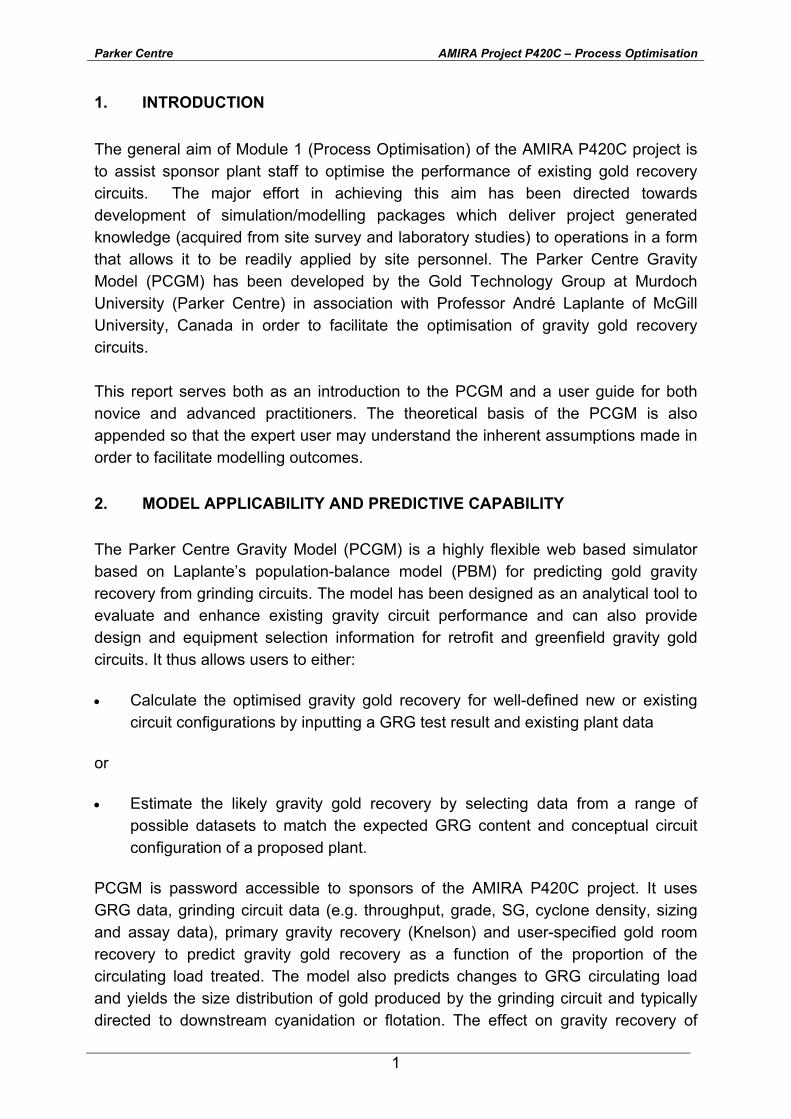
The general aim of Module 1 (Process Optimisation) of the AMIRA P420C project is to assist sponsor plant staff to optimise the performance of existing gold recovery circuits. The major effort in achieving this aim has been directed towards development of simulation/modelling packages which deliver project generated knowledge (acquired from site survey and laboratory studies) to operations in a form that allows it to be readily applied by site personnel. The Parker Centre Gravity Model (PCGM) has been developed by the Gold Technology Group at Murdoch University (Parker Centre) in association with Professor André Laplante of McGill University, Canada in order to facilitate the optimisation of gravity gold recovery circuits. This report serves both as an introduction to the PCGM and a user guide for both novice and advanced practitioners. The theoretical basis of the PCGM is also appended so that the expert user may understand the inherent assumptions made in order to facilitate modelling outcomes.

2. MODEL APPLICABILITY AND PREDICTIVE CAPABILITY

The Parker Centre Gravity Model (PCGM) is a highly flexible web based simulator based on Laplante’s population-balance model (PBM) for predicting gold gravity recovery from grinding circuits. The model has been designed as an analytical tool to evaluate and enhance existing gravity circuit performance and can also provide design and equipment selection information for retrofit and greenfield gravity gold circuits. It thus allows users to either:

• Calculate the optimised gravity gold recovery for well-defined new or existing circuit configurations by inputting a GRG test result and existing plant data

or

• Estimate the likely gravity gold recovery by selecting data from a range of possible datasets to match the expected GRG content and conceptual circuit configuration of a proposed plant.

PCGM is password accessible to sponsors of the AMIRA P420C project. It uses GRG data, grinding circuit data (e.g. throughput, grade, SG, cyclone density, sizing and assay data), primary gravity recovery (Knelson) and user-specified gold room recovery to predict gravity gold recovery as a function of the proportion of the circulating load treated. The model also predicts changes to GRG circulating load and yields the size distribution of gold produced by the grinding circuit and typically directed to downstream cyanidation or flotation. The effect on gravity recovery of


2

altering the bleed stream treated, the number (or type) of gravity device installed, the cyclone performance (d50 or separation sharpness) and the ore GRG content or size distribution can also be assessed rapidly and accurately depending on what input data is available and what assumptions must be made. The simulation results page shows the recommended number of concentrators required to treat varying proportions of the circulating load, and the best combinations of Knelson 20, 30, or 48 inch units are suggested for each circuit size. The rationale behind offering a range of circuit options is to demonstrate clearly to the user that the link between the recovery effort and the total amount of GRG recovered is highly non-linear [2]. By matching design and operating costs to the predicted amount of gold recovered, the user can approach the optimum economic size of the gravity circuit [3].

The gravity model is currently only applicable to Knelson Concentrator based gravity circuits but further research in AMIRA P420C aims to incorporate other gravity devices.

3. CONCEPTUAL BASIS OF PARKER CENTRE GRAVITY MODEL

3.1 Gravity Recoverable Gold

“Gravity Recoverable Gold” (GRG) content of an ore is an essential concept in the development of the Parker Centre Gravity Model. André Laplante defines GRG as:

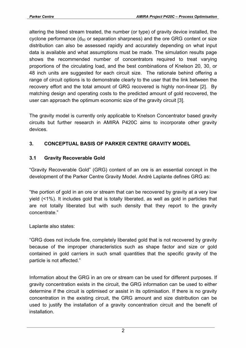
“the portion of gold in an ore or stream that can be recovered by gravity at a very low yield (<1%). It includes gold that is totally liberated, as well as gold in particles that are not totally liberated but with such density that they report to the gravity concentrate.” Laplante also states: “GRG does not include fine, completely liberated gold that is not recovered by gravity because of the improper characteristics such as shape factor and size or gold contained in gold carriers in such small quantities that the specific gravity of the particle is not affected.”

Information about the GRG in an ore or stream can be used for different purposes. If gravity concentration exists in the circuit, the GRG information can be used to either determine if the circuit is optimised or assist in its optimisation. If there is no gravity concentration in the existing circuit, the GRG amount and size distribution can be used to justify the installation of a gravity concentration circuit and the benefit of installation.


3

A standardised test to determine GRG content of an ore was developed at McGill University and involves three stages of progressive liberation and recovery of gold-bearing particles using a laboratory centrifuge unit (Knelson Concentrator MD3 - manual discharge, rotor of 3” nominal diameter). Details of the GRG test procedure are given in Appendix 1. Actual plant recovery is always inferior to measured GRG because test conditions are designed to yield maximum theoretical GRG recovery. A simpler single stage GRG test performed at the final grind size and suitable for more routine application was developed during the AMIRA P420B research program.

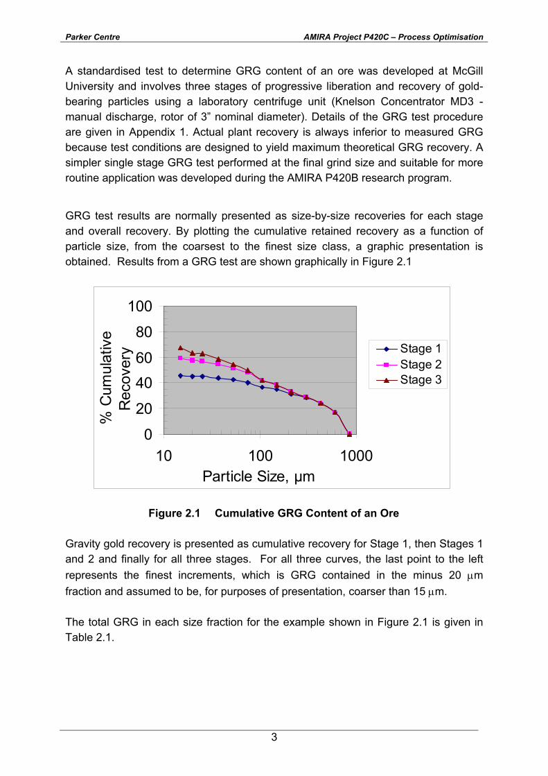
GRG test results are normally presented as size-by-size recoveries for each stage and overall recovery. By plotting the cumulative retained recovery as a function of particle size, from the coarsest to the finest size class, a graphic presentation is obtained. Results from a GRG test are shown graphically in Figure 2.1

Figure 2.1 Cumulative GRG Content of an Ore

Gravity gold recovery is presented as cumulative recovery for Stage 1, then Stages 1 and 2 and finally for all three stages. For all three curves, the last point to the left represents the finest increments, which is GRG contained in the minus 20 µm fraction and assumed to be, for purposes of presentation, coarser than 15 µm. The total GRG in each size fraction for the example shown in Figure 2.1 is given in Table 2.1.

0

20

4060

80

100

10 100 1000Particle Size, µm

% C

umul

ativ

eR

ecov

ery Stage 1

Stage 2Stage 3


4

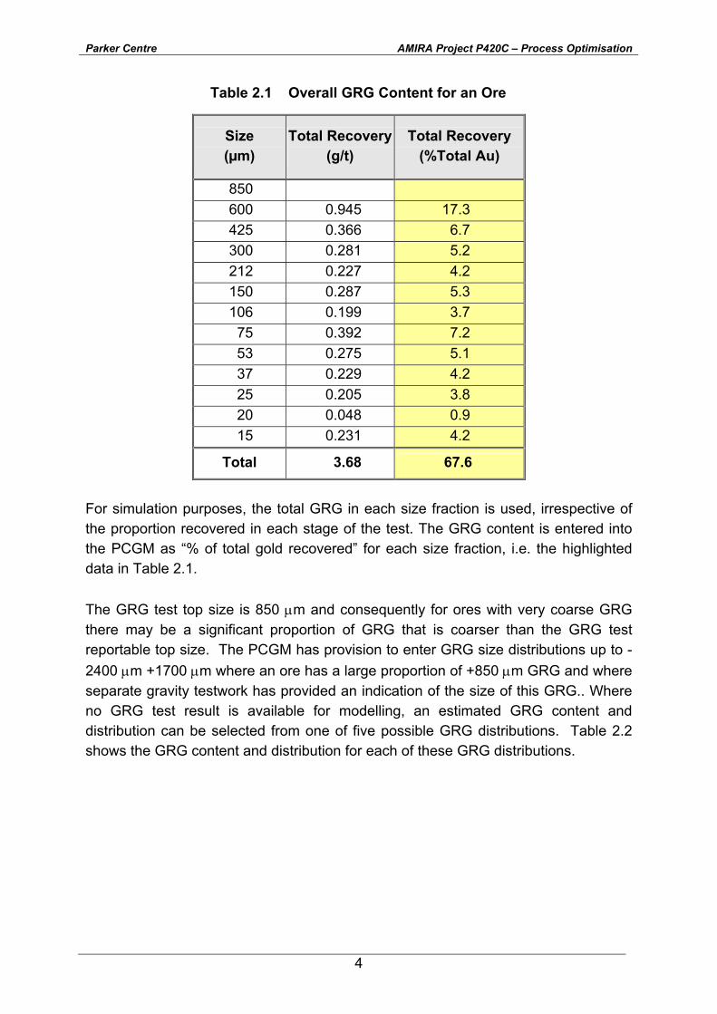
Table 2.1 Overall GRG Content for an Ore

Size (µm)

Total Recovery(g/t)

Total Recovery (%Total Au)

850 600 0.945 17.3 425 0.366 6.7 300 0.281 5.2 212 0.227 4.2 150 0.287 5.3 106 0.199 3.7 75 0.392 7.2 53 0.275 5.1 37 0.229 4.2 25 0.205 3.8 20 0.048 0.9 15 0.231 4.2

Total 3.68 67.6

For simulation purposes, the total GRG in each size fraction is used, irrespective of the proportion recovered in each stage of the test. The GRG content is entered into the PCGM as “% of total gold recovered” for each size fraction, i.e. the highlighted data in Table 2.1. The GRG test top size is 850 µm and consequently for ores with very coarse GRG there may be a significant proportion of GRG that is coarser than the GRG test reportable top size. The PCGM has provision to enter GRG size distributions up to -2400 µm +1700 µm where an ore has a large proportion of +850 µm GRG and where separate gravity testwork has provided an indication of the size of this GRG.. Where no GRG test result is available for modelling, an estimated GRG content and distribution can be selected from one of five possible GRG distributions. Table 2.2 shows the GRG content and distribution for each of these GRG distributions.


5

Table 2.2 Estimated GRG Content for Varying Gold Particle Sizes

Size Gold Particle Size

(µm) Very Fine (P80~80µm)

Fine (P80~100µm)

Average (P80~120µm)

Coarse (P80~200µm)

Very Coarse

(P80~350µm)600 0.01 0.04 0.66 2.16 7.36 425 0.11 0.31 2.05 4.23 10.62 300 0.58 1.21 4.07 6.13 11.31 212 1.62 2.80 5.90 7.21 10.25 150 2.95 4.51 6.92 7.36 8.41 106 3.93 5.56 6.90 6.71 6.38 75 4.28 5.76 6.22 5.72 4.64 53 4.15 5.41 5.34 4.74 3.36 37 3.78 4.83 4.50 3.92 2.45 25 3.58 4.54 4.07 3.52 1.93 15 11.73 9.96 10.56 10.97 10.03

Total 36.73 44.94 57.19 62.68 76.73

3.2 Gold Behaviour and Population Balance Model (PBM)

The Parker Centre Gravity Model is a phenomenological model, the major computational component of which is a size by size derived population-balance model (PBM) developed by Laplante et al. The GRG population balance model incorporates the concepts of gold liberation, breakage (grinding) and classification behaviour and these aspects are described in more detail in Appendix 2. The 5 matrix components used and the derivation of the PBM is explained in Appendix 3, using firstly a simplified single size class approach and then as it is actually used to predict gravity recovery in the full size-class model.

The PBM approach has now been largely validated with predictions of circulating loads and gold recoveries observed in actual plants having been shown by Laplante to be acceptably accurate even though one of the most important variables (GRG content) is derived from a laboratory test.

A number of important assumptions have been made in development of the PCGM in order to give it the inherent flexibility necessary to predict gravity recovery from a wide range of data input possibilities. The various assumptions are described in Appendices 2 and 3.


6

4.0 USING THE GRAVITY MODEL

This section acts as a user guide and provides a step by step description of the Parker Centre Gravity Model. Necessary data required for each stage of the calculation sequence is outlined and “screen shots” of each input screen associated with the model are incorporated. Example calculations of gravity gold recovery from typical circuit configurations are provided and the corresponding results produced by the model are described and interpreted.

4.1 Model Access

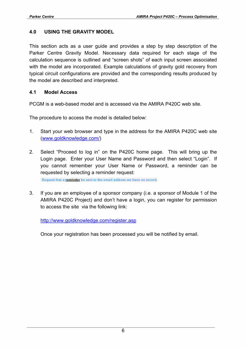
PCGM is a web-based model and is accessed via the AMIRA P420C web site. The procedure to access the model is detailed below: 1. Start your web browser and type in the address for the AMIRA P420C web site

(www.goldknowledge.com/) 2. Select “Proceed to log in” on the P420C home page. This will bring up the

Login page. Enter your User Name and Password and then select “Login”. If you cannot remember your User Name or Password, a reminder can be requested by selecting a reminder request:

3. If you are an employee of a sponsor company (i.e. a sponsor of Module 1 of the

AMIRA P420C Project) and don’t have a login, you can register for permission to access the site via the following link:

http://www.goldknowledge.com/register.asp Once your registration has been processed you will be notified by email.


7

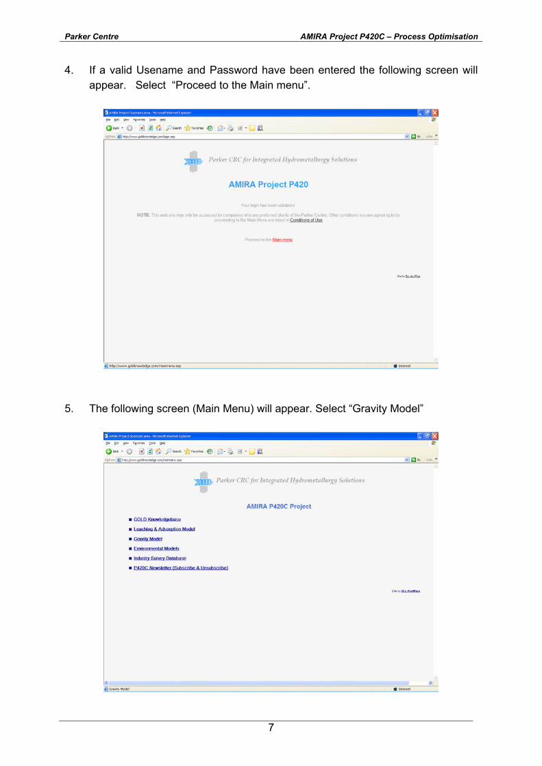
4. If a valid Usename and Password have been entered the following screen will appear. Select “Proceed to the Main menu”.

5. The following screen (Main Menu) will appear. Select “Gravity Model”


8

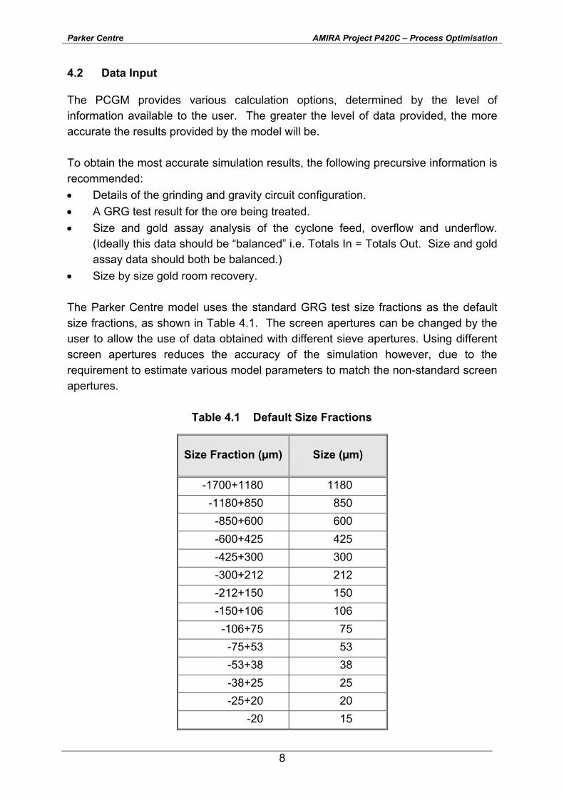
4.2 Data Input

The PCGM provides various calculation options, determined by the level of information available to the user. The greater the level of data provided, the more accurate the results provided by the model will be. To obtain the most accurate simulation results, the following precursive information is recommended: • Details of the grinding and gravity circuit configuration. • A GRG test result for the ore being treated. • Size and gold assay analysis of the cyclone feed, overflow and underflow.

(Ideally this data should be “balanced” i.e. Totals In = Totals Out. Size and gold assay data should both be balanced.)

• Size by size gold room recovery. The Parker Centre model uses the standard GRG test size fractions as the default size fractions, as shown in Table 4.1. The screen apertures can be changed by the user to allow the use of data obtained with different sieve apertures. Using different screen apertures reduces the accuracy of the simulation however, due to the requirement to estimate various model parameters to match the non-standard screen apertures.

Table 4.1 Default Size Fractions

Size Fraction (µm) Size (µm)

-1700+1180 1180 -1180+850 850

-850+600 600 -600+425 425 -425+300 300 -300+212 212 -212+150 150 -150+106 106 -106+75 75 -75+53 53 -53+38 38 -38+25 25 -25+20 20

-20 15


9

If no GRG test results are available the model can estimate the GRG content for your ore using one of the following methods. • If size and Au assay analyses for the cyclone feed, overflow and underflow are

available the GRG content is estimated from these data. • If cyclone size and assay data is unavailable, GRG content can be selected

from one of five default GRG estimates provided. It should be noted that simulations based on this method have the lowest level of accuracy. Further details are provided in Appendix 2.

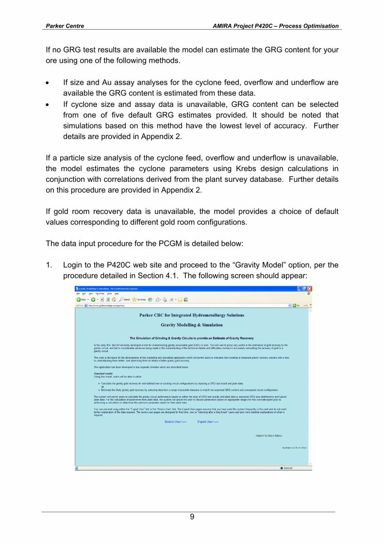
If a particle size analysis of the cyclone feed, overflow and underflow is unavailable, the model estimates the cyclone parameters using Krebs design calculations in conjunction with correlations derived from the plant survey database. Further details on this procedure are provided in Appendix 2. If gold room recovery data is unavailable, the model provides a choice of default values corresponding to different gold room configurations. The data input procedure for the PCGM is detailed below: 1. Login to the P420C web site and proceed to the “Gravity Model” option, per the

procedure detailed in Section 4.1. The following screen should appear:


10

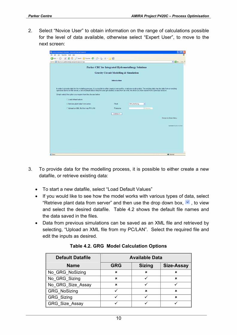
2. Select “Novice User” to obtain information on the range of calculations possible for the level of data available, otherwise select “Expert User”, to move to the next screen:

3. To provide data for the modelling process, it is possible to either create a new

datafile, or retrieve existing data:

• To start a new datafile, select “Load Default Values” • If you would like to see how the model works with various types of data, select

“Retrieve plant data from server” and then use the drop down box, , to view and select the desired datafile. Table 4.2 shows the default file names and the data saved in the files.

• Data from previous simulations can be saved as an XML file and retrieved by selecting, “Upload an XML file from my PC/LAN”. Select the required file and edit the inputs as desired.

Table 4.2. GRG Model Calculation Options

Default Datafile Available Data

Name GRG Sizing Size-Assay No_GRG_NoSizing No_GRG_Sizing No_GRG_Size_Assay GRG_NoSizing GRG_Sizing GRG_Size_Assay


11

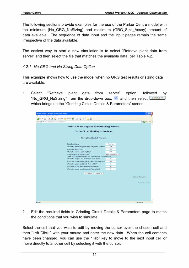
The following sections provide examples for the use of the Parker Centre model with the minimum (No_GRG_NoSizing) and maximum (GRG_Size_Assay) amount of data available. The sequence of data input and the input pages remain the same irrespective of the data available. The easiest way to start a new simulation is to select “Retrieve plant data from server” and then select the file that matches the available data, per Table 4.2. 4.2.1 No GRG and No Sizing Data Option This example shows how to use the model when no GRG test results or sizing data are available. 1. Select “Retrieve plant data from server” option, followed by

“No_GRG_NoSizing” from the drop-down box, , and then select , which brings up the “Grinding Circuit Details & Parameters” screen:

2. Edit the required fields in Grinding Circuit Details & Parameters page to match the conditions that you wish to simulate.

Select the cell that you wish to edit by moving the cursor over the chosen cell and then “Left Click ” with your mouse and enter the new data. When the cell contents have been changed, you can use the “Tab” key to move to the next input cell or move directly to another cell by selecting it with the cursor.


12

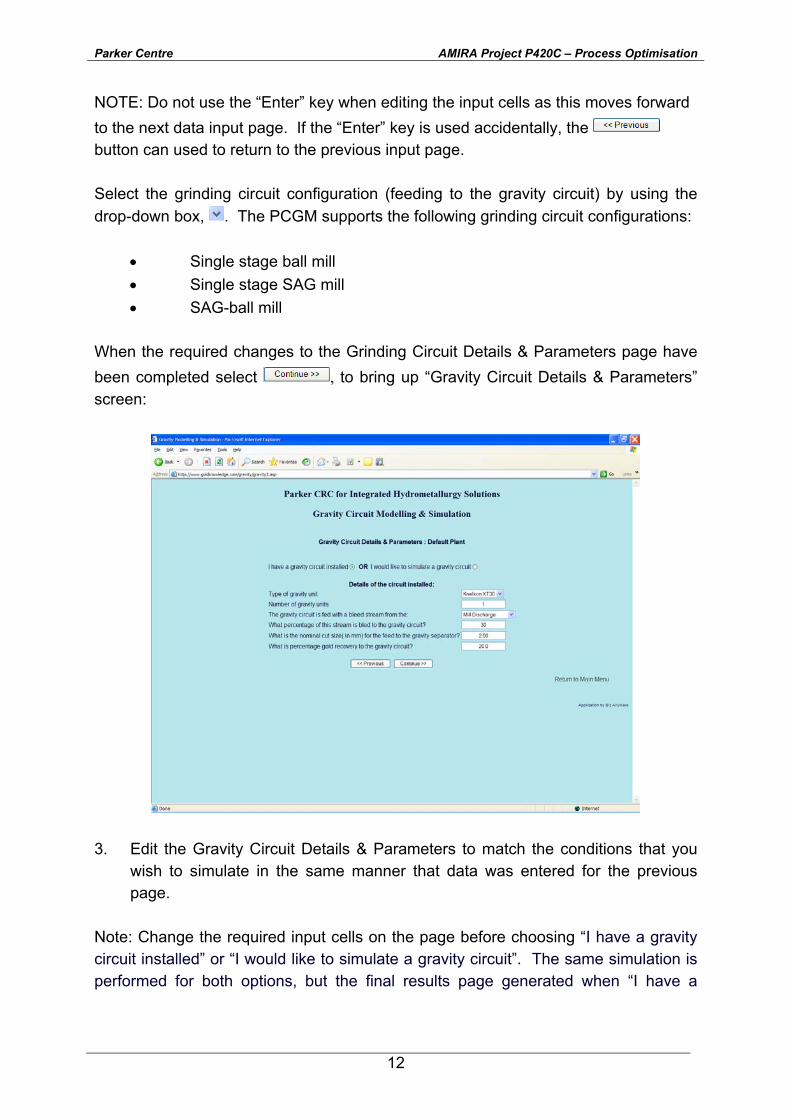
NOTE: Do not use the “Enter” key when editing the input cells as this moves forward to the next data input page. If the “Enter” key is used accidentally, the button can used to return to the previous input page. Select the grinding circuit configuration (feeding to the gravity circuit) by using the drop-down box, . The PCGM supports the following grinding circuit configurations:

• Single stage ball mill • Single stage SAG mill • SAG-ball mill

When the required changes to the Grinding Circuit Details & Parameters page have been completed select , to bring up “Gravity Circuit Details & Parameters” screen:

3. Edit the Gravity Circuit Details & Parameters to match the conditions that you wish to simulate in the same manner that data was entered for the previous page.

Note: Change the required input cells on the page before choosing “I have a gravity circuit installed” or “I would like to simulate a gravity circuit”. The same simulation is performed for both options, but the final results page generated when “I have a


13

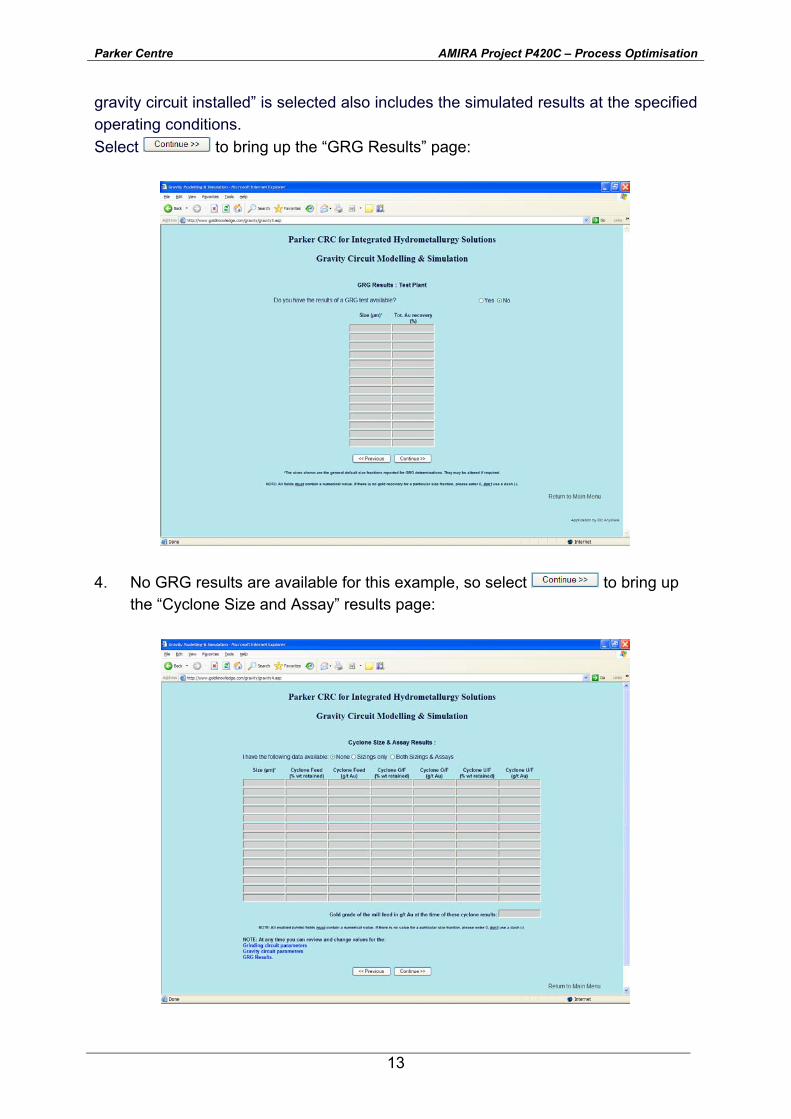
gravity circuit installed” is selected also includes the simulated results at the specified operating conditions. Select to bring up the “GRG Results” page:

4. No GRG results are available for this example, so select to bring up the “Cyclone Size and Assay” results page:


14

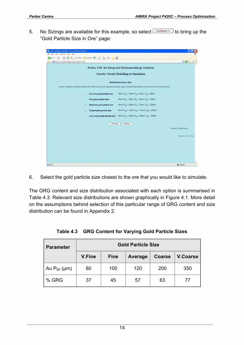
5. No Sizings are available for this example, so select to bring up the “Gold Particle Size in Ore” page:

6. Select the gold particle size closest to the ore that you would like to simulate.

The GRG content and size distribution associated with each option is summarised in Table 4.3. Relevant size distributions are shown graphically in Figure 4.1. More detail on the assumptions behind selection of this particular range of GRG content and size distribution can be found in Appendix 2.

Table 4.3 GRG Content for Varying Gold Particle Sizes

Parameter Gold Particle Size

V.Fine Fine Average Coarse V.Coarse

Au P80 (µm) 80 100 120 200 350

% GRG 37 45 57 63 77


15

0

10

20

30

40

50

60

70

80

90

10 100 1000

Size (µm)

Cum

ulat

ive

GRG

Rec

over

y (%

)V. FineFineAveCoarseV. Coarse

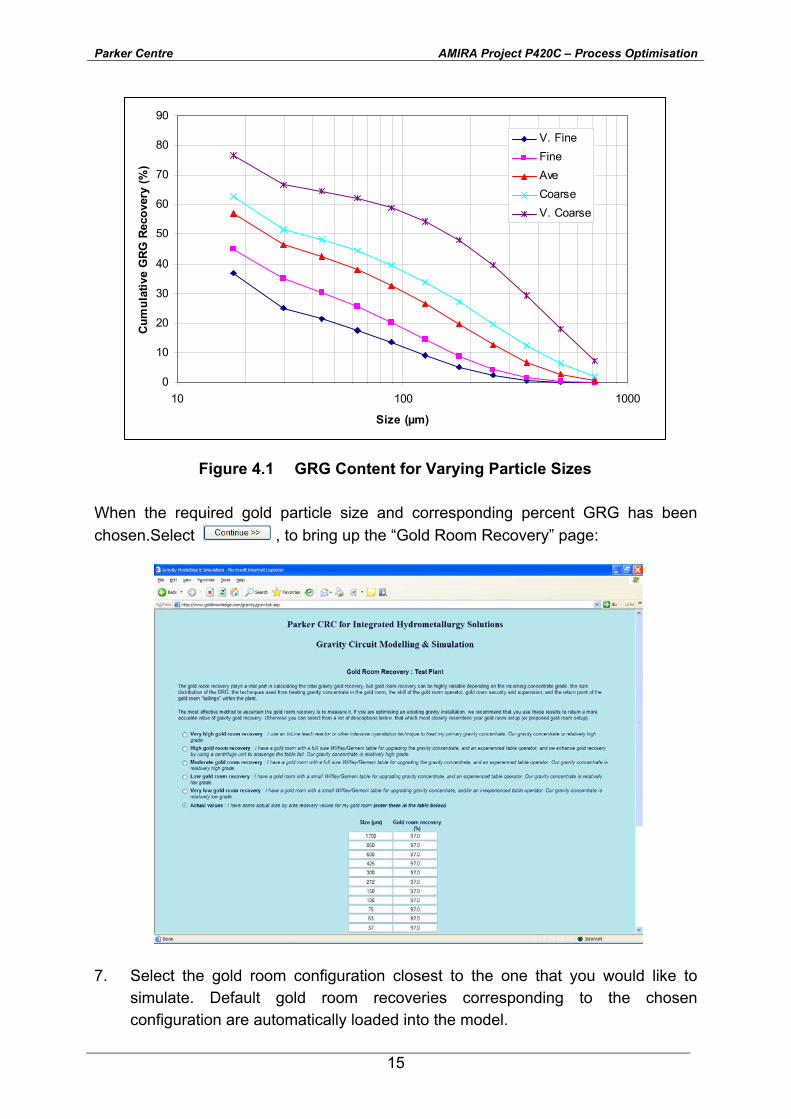
Figure 4.1 GRG Content for Varying Particle Sizes When the required gold particle size and corresponding percent GRG has been chosen.Select , to bring up the “Gold Room Recovery” page:

7. Select the gold room configuration closest to the one that you would like to

simulate. Default gold room recoveries corresponding to the chosen configuration are automatically loaded into the model.


16

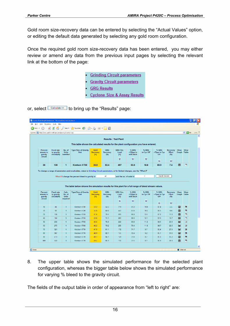
Gold room size-recovery data can be entered by selecting the “Actual Values” option, or editing the default data generated by selecting any gold room configuration. Once the required gold room size-recovery data has been entered, you may either review or amend any data from the previous input pages by selecting the relevant link at the bottom of the page:

or, select to bring up the “Results” page:

8. The upper table shows the simulated performance for the selected plant

configuration, whereas the bigger table below shows the simulated performance for varying % bleed to the gravity circuit.

The fields of the output table in order of appearance from “left to right” are:


17

• Percent stream to gravity circuit The “Percent stream to gravity circuit” is the percent mass of the treated stream that feeds to the primary gravity recovery stage.

• Feed rate to gravity circuit(t/h)

The “Feed rate to gravity circuit” is the mass flow rate of solids to the primary gravity recovery stage.

• Calc. No. of Units required

The “Calc. No. of Units” is the number of primary gravity concentrators determined by the model for the specified feed rate.

• Type/Size of Gravity Unit

The “Type/Size of Gravity Unit” is model and size of the primary gravity concentrators determined by the model for the specified feed rate.

• Gold Recovery (%)

The “Gold Recovery” is the calculated gold recovery at the specified feed rate and the selected number and size of primary concentrators.

• GRG Recovery (%)

The “GRG Recovery” is the calculated GRG recovery at the specified feed rate and the selected number and size of primary concentrators.

• GRG Circ. Load (%)

The “GRG Circ. Load” is the GRG Circulating Load, and is calculated in a similar fashion to the solid mass circulating load. The expression used in the calculation is:

% GRG C.L = (GRG mass flow in recycle stream x 100)/GRG in circuit feed The GRG Circulating Load is affected by the following:

GRG size distribution - The GRG circulating load will increase if the GRG size

distribution becomes coarser. Cyclone Separation Efficiency - The GRG circulating load will increase if the

cyclone d50 becomes finer or the separation sharpness increases. Recovery Effort - The GRG circulating load decreases with increasing

recovery effort.


18

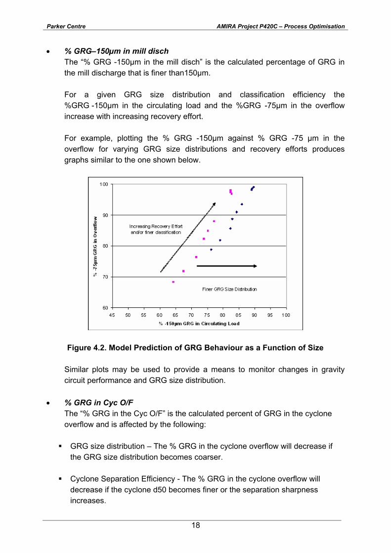
• % GRG–150µm in mill disch The “% GRG -150µm in the mill disch” is the calculated percentage of GRG in the mill discharge that is finer than150µm.

For a given GRG size distribution and classification efficiency the %GRG -150µm in the circulating load and the %GRG -75µm in the overflow increase with increasing recovery effort.

For example, plotting the % GRG -150µm against % GRG -75 µm in the overflow for varying GRG size distributions and recovery efforts produces graphs similar to the one shown below.

Figure 4.2. Model Prediction of GRG Behaviour as a Function of Size

Similar plots may be used to provide a means to monitor changes in gravity circuit performance and GRG size distribution.

• % GRG in Cyc O/F

The “% GRG in the Cyc O/F” is the calculated percent of GRG in the cyclone overflow and is affected by the following:

GRG size distribution – The % GRG in the cyclone overflow will decrease if

the GRG size distribution becomes coarser.

Cyclone Separation Efficiency - The % GRG in the cyclone overflow will decrease if the cyclone d50 becomes finer or the separation sharpness increases.


19

Recovery Effort - The % GRG in the cyclone overflow decreases with increasing recovery effort.

Increasing % GRG in the cyclone O/F may result in decreased leach recoveries

• % GRG –75µm in Cyc O/F

The “% GRG -75µm in the Cyc O/F” is the calculated percent of the GRG in the cyclone overflow that is finer than 75 µm.

The % GRG -75 µm in the cyclone overflow is affected by the following:

GRG size distribution – The % GRG -75 µm in the cyclone overflow decreases

slightly as the GRG size distribution becomes coarser. Cyclone Separation Efficiency - The % GRG -75 µm in the cyclone overflow

will increase if the cyclone d50 becomes finer or the separation sharpness increases.

Recovery Effort - The % GRG -75 µm in the cyclone overflow increases with increasing recovery effort.

Decreasing “% GRG -75µm in the Cyc O/F” (i.e. coarser GRG in the cyclone overflow) may result in lower leach recoveries.

• Recovery Effort (%)

The “Recovery Effort” is obtained by multiplying the (fractional) recovery of each stage of the GRG recovery process. It provides a measure of the overall efficiency of the circuit. For example, when treating 30% of the circulating load, with 40 % recovery from the primary concentrator and 90 % goldroom recovery, the recovery effort is:

Recovery Effort = 0.3 x 0.4 x 0.9 = 0.108 x 100 = 10.8 %

• View Graph

View Graph shows a graph of the size-by-size results for the selected case. • View Table

View Table shows table of the size-by-size results for the selected case.

Selecting the help button in any of the columns provides a description of the data in the corresponding field.

Data input for the simulation can be saved for future use by selecting . The XML file can then be retrieved using the option at the


20

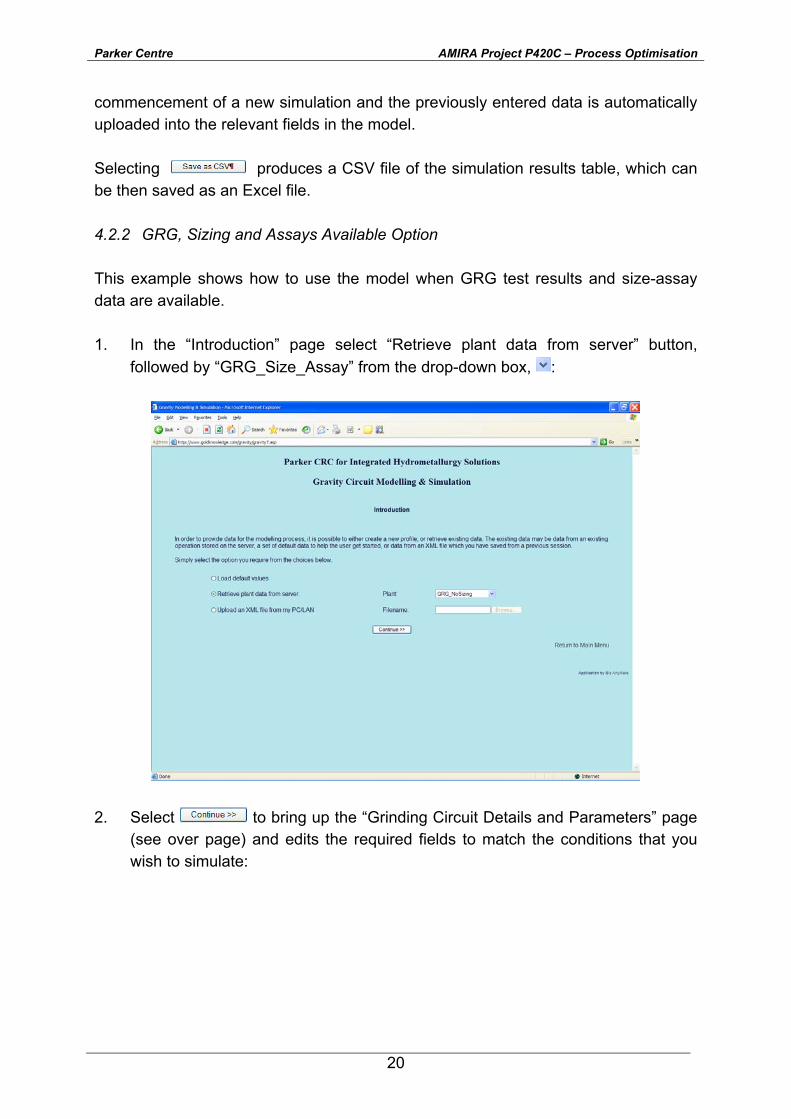
commencement of a new simulation and the previously entered data is automatically uploaded into the relevant fields in the model. Selecting produces a CSV file of the simulation results table, which can be then saved as an Excel file. 4.2.2 GRG, Sizing and Assays Available Option This example shows how to use the model when GRG test results and size-assay data are available. 1. In the “Introduction” page select “Retrieve plant data from server” button,

followed by “GRG_Size_Assay” from the drop-down box, :

2. Select to bring up the “Grinding Circuit Details and Parameters” page

(see over page) and edits the required fields to match the conditions that you wish to simulate:


21

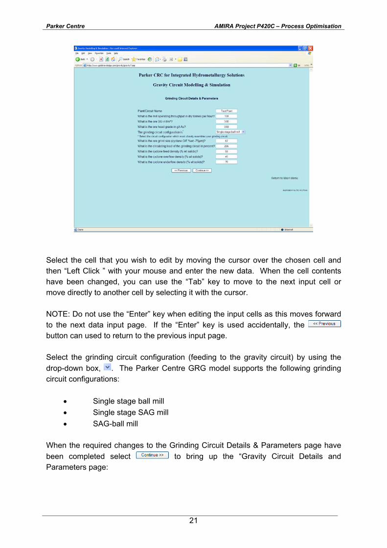
Select the cell that you wish to edit by moving the cursor over the chosen cell and then “Left Click ” with your mouse and enter the new data. When the cell contents have been changed, you can use the “Tab” key to move to the next input cell or move directly to another cell by selecting it with the cursor. NOTE: Do not use the “Enter” key when editing the input cells as this moves forward to the next data input page. If the “Enter” key is used accidentally, the button can used to return to the previous input page. Select the grinding circuit configuration (feeding to the gravity circuit) by using the drop-down box, . The Parker Centre GRG model supports the following grinding circuit configurations:

• Single stage ball mill • Single stage SAG mill • SAG-ball mill

When the required changes to the Grinding Circuit Details & Parameters page have been completed select to bring up the “Gravity Circuit Details and Parameters page:


22

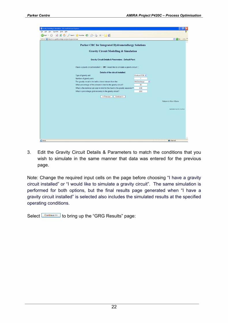
3. Edit the Gravity Circuit Details & Parameters to match the conditions that you wish to simulate in the same manner that data was entered for the previous page.

Note: Change the required input cells on the page before choosing “I have a gravity circuit installed” or “I would like to simulate a gravity circuit”. The same simulation is performed for both options, but the final results page generated when “I have a gravity circuit installed” is selected also includes the simulated results at the specified operating conditions. Select to bring up the “GRG Results” page:


23

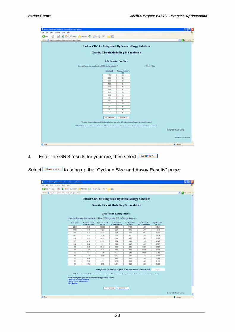
4. Enter the GRG results for your ore, then select Select to bring up the “Cyclone Size and Assay Results” page:


24

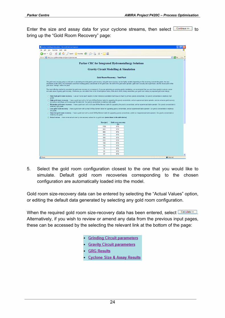
Enter the size and assay data for your cyclone streams, then select to bring up the “Gold Room Recovery” page:

5. Select the gold room configuration closest to the one that you would like to

simulate. Default gold room recoveries corresponding to the chosen configuration are automatically loaded into the model.

Gold room size-recovery data can be entered by selecting the “Actual Values” option, or editing the default data generated by selecting any gold room configuration. When the required gold room size-recovery data has been entered, select . Alternatively, if you wish to review or amend any data from the previous input pages, these can be accessed by the selecting the relevant link at the bottom of the page:


25

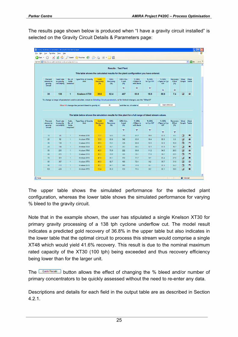
The results page shown below is produced when “I have a gravity circuit installed” is selected on the Gravity Circuit Details & Parameters page:

The upper table shows the simulated performance for the selected plant configuration, whereas the lower table shows the simulated performance for varying % bleed to the gravity circuit. Note that in the example shown, the user has stipulated a single Knelson XT30 for primary gravity processing of a 138 tph cyclone underflow cut. The model result indicates a predicted gold recovery of 36.8% in the upper table but also indicates in the lower table that the optimal circuit to process this stream would comprise a single XT48 which would yield 41.6% recovery. This result is due to the nominal maximum rated capacity of the XT30 (100 tph) being exceeded and thus recovery efficiency being lower than for the larger unit. The button allows the effect of changing the % bleed and/or number of primary concentrators to be quickly assessed without the need to re-enter any data. Descriptions and details for each field in the output table are as described in Section 4.2.1.


26

5. CONCLUSIONS

The Parker Centre Gravity Model is extremely flexible. Although the most accurate prediction of gravity circuit performance requires input of a substantial data set covering GRG test results and extensive stream sizing and assay details from an existing circuit, the gravity model can still generate indicative data from quite scanty ore and circuit detail. If no GRG result is available but cyclone stream size assays are known, a very good estimate of the ore GRG can be calculated by the model. If neither ore GRG nor cyclone data are available, a less accurate estimate of GRG is derived from user specified “average” gold particle size in ore. Similarly cyclone performance for ore and GRG (d50 and separation sharpness) can be either calculated from stream sizing and assay data or extrapolated from mill grind size and cyclone densities. The model has been operational since mid 2004 although plant data has not yet been extensively tested. Further expansion of the simulator is planned, including the incorporation of other recovery devices, such as the Falcon Concentrator, In-Line Pressure Jig, and flash flotation or contact cells. The use of the simulator as a diagnostic tool for troubleshooting gravity circuits is also proposed.

6. ACKNOWLEDGEMENTS

The assistance of staff from the various sponsor sites that participated in the AMIRA P420B Project is gratefully acknowledged. In addition, the authors wish to thank Xhixian Xiao for providing a copy of his well written and comprehensive thesis, which provided an excellent reference for the development of the model and the theory detailed in this guide. Finally, the authors would like to acknowledge Mr William Staunton, Professor André Laplante, the staff and students of the AMIRA P420B project and its sponsors for the work and the funding which developed the methodology and made the Parker Centre Gravity Model possible.


27

7. REFERENCES

1 Laplante, A. R., Woodcock, F., and Noaparast, M., 1994, “Predicting Gold Recovery by Gravity”, Proceedings, Annual Meeting of SME, Albuquerque, Paper 94-158.

2 Banisi, S., Laplante, A. R., and Marois, J., 1991, “The behaviour of Gold in

Hemlo Mines Ltd. Grinding Circuit”, CIM Bulletin, Vol. 84(955), pp. 72-78. 3 Austin, L. G., Luckie, P. T., and Klimpel, R. R., 1984, “Process Engineering of

Size Reduction: Ball Milling”, Pub. SME, Littleton, CO. 4 Laplante, A. R., Finch, J. A., and del Villar, R., 1987, “Simplification of the

Grinding Equation for Plant Simulation”, Trans. Inst. Min. Metall. (London), Sect. C., June, Vol. 96, pp. C 108-112.

5 Noaparast, M., 1997, “The Behavior of Malleable Metals in Tumbling Mills.”

Master of Engineering Thesis, McGill University, Montréal 6 Plitt, L. R., 1976, “A Mathematical Model of the Hydrocyclone Classifier”, CIM

Bull., Vol. 69, No. 776, Dec., pp. 114-123. 7 Luckie, P.T. and Austin, L.G., “A Review Introduction of the Solution of the

Grinding Equation by Digital Computation”, Min. Sci. Eng., Vol. 4(2), April 1972, pp. 24-52.

8 Xiao, X "Developing Simple Regressions For Predicting Gold Gravity Recovery

in Grinding Circuit", Zhixian Xiao,M.Eng. Thesis, McGill University, September 2001.

9 Arterburn, R.A., “The Sizing and Selection of Hydrocyclones”, Krebs Engineers,

www.krebs.com/documents/83_sizing_select_cyclones.pdf 10 Laplante, A. R., 1999, Course Notes, “Modeling and Control of Mineral

Processing Systems”, Mining and Metallurgical Engineering Department, McGill University.

11 Laplante, A.R., “Gravity Gold Workshop”, A.J. Parker C.R.C, Perth, May 12-13,

2003


28

APPENDIX 1 - GRG TEST PROCEDURE

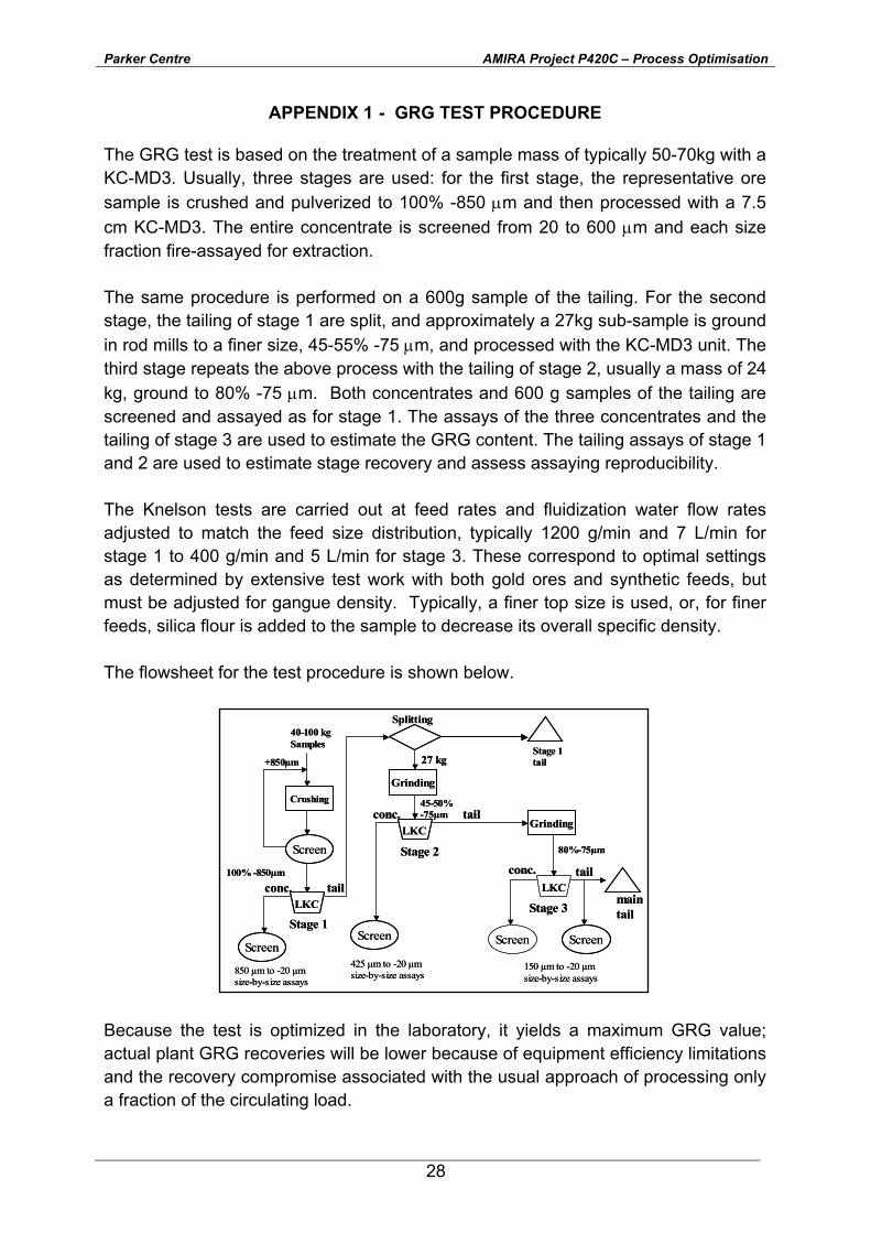
The GRG test is based on the treatment of a sample mass of typically 50-70kg with a KC-MD3. Usually, three stages are used: for the first stage, the representative ore sample is crushed and pulverized to 100% -850 µm and then processed with a 7.5 cm KC-MD3. The entire concentrate is screened from 20 to 600 µm and each size fraction fire-assayed for extraction. The same procedure is performed on a 600g sample of the tailing. For the second stage, the tailing of stage 1 are split, and approximately a 27kg sub-sample is ground in rod mills to a finer size, 45-55% -75 µm, and processed with the KC-MD3 unit. The third stage repeats the above process with the tailing of stage 2, usually a mass of 24 kg, ground to 80% -75 µm. Both concentrates and 600 g samples of the tailing are screened and assayed as for stage 1. The assays of the three concentrates and the tailing of stage 3 are used to estimate the GRG content. The tailing assays of stage 1 and 2 are used to estimate stage recovery and assess assaying reproducibility. The Knelson tests are carried out at feed rates and fluidization water flow rates adjusted to match the feed size distribution, typically 1200 g/min and 7 L/min for stage 1 to 400 g/min and 5 L/min for stage 3. These correspond to optimal settings as determined by extensive test work with both gold ores and synthetic feeds, but must be adjusted for gangue density. Typically, a finer top size is used, or, for finer feeds, silica flour is added to the sample to decrease its overall specific density. The flowsheet for the test procedure is shown below.

Splitting

Stage 1tail

425 µm to -20 µmsize-by-size assays

LKCtail

Grinding

Screen

27 kg

45-50%-75µmconc.

Stage 2

40-100 kg Samples

Crushing

Screen

+850µm

tailconc.100% -850µm

LKC

Screen

Stage 1


Screen

Grinding

LKC

Screen

80%-75µm

conc. tail

Stage 3maintail


Splitting

Stage 1tail


LKCtail

Grinding

Screen

27 kg

45-50%-75µmconc.

Stage 2

40-100 kg Samples

Crushing

Screen

+850µm

tailconc.100% -850µm

LKC

Screen

Stage 1


Screen

Grinding

LKC

Screen

80%-75µm

conc. tail

Stage 3maintail


Because the test is optimized in the laboratory, it yields a maximum GRG value; actual plant GRG recoveries will be lower because of equipment efficiency limitations and the recovery compromise associated with the usual approach of processing only a fraction of the circulating load.


29

APPENDIX 2 - THEORETICAL CONSIDERATIONS

A2.1 Behaviour of Gold in Comminution Circuits

The malleability of gold results in differences in behaviour between it and other minerals in grinding circuits. Banisi (2) investigated the grinding behaviour of gold and silica in a laboratory mill to determine their respective breakage and selection functions.

A2.1.1 The Breakage Function

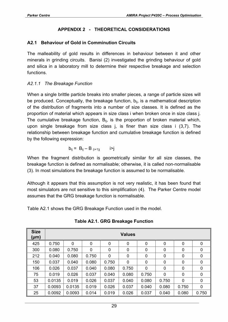
When a single brittle particle breaks into smaller pieces, a range of particle sizes will be produced. Conceptually, the breakage function, bij, is a mathematical description of the distribution of fragments into a number of size classes. It is defined as the proportion of material which appears in size class i when broken once in size class j. The cumulative breakage function, Bij, is the proportion of broken material which, upon single breakage from size class j, is finer than size class i (3,7). The relationship between breakage function and cumulative breakage function is defined by the following expression: bij = Bij – B (i+1)j i>j When the fragment distribution is geometrically similar for all size classes, the breakage function is defined as normalisable; otherwise, it is called non-normalisable (3). In most simulations the breakage function is assumed to be normalisable. Although it appears that this assumption is not very realistic, it has been found that most simulators are not sensitive to this simplification (4). The Parker Centre model assumes that the GRG breakage function is normalisable. Table A2.1 shows the GRG Breakage Function used in the model.

Table A2.1. GRG Breakage Function

Size (µm) Values

425 0.750 0 0 0 0 0 0 0 0 300 0.080 0.750 0 0 0 0 0 0 0 212 0.040 0.080 0.750 0 0 0 0 0 0 150 0.037 0.040 0.080 0.750 0 0 0 0 0 106 0.026 0.037 0.040 0.080 0.750 0 0 0 0 75 0.019 0.026 0.037 0.040 0.080 0.750 0 0 0 53 0.0135 0.019 0.026 0.037 0.040 0.080 0.750 0 0 37 0.0093 0.0135 0.019 0.026 0.037 0.040 0.080 0.750 0 25 0.0092 0.0093 0.014 0.019 0.026 0.037 0.040 0.080 0.750


30

A2.1.2 The Selection Function

The selection function or specific rate of breakage, is a measure of grinding process kinetics. In other words, it is an indication of how fast the material breaks. There is ample experimental evidence that batch grinding kinetics follow first order with respect to the disappearance of material from a given size class due to breakage (3):

)().()( tMtSdt

tdMii

i −=

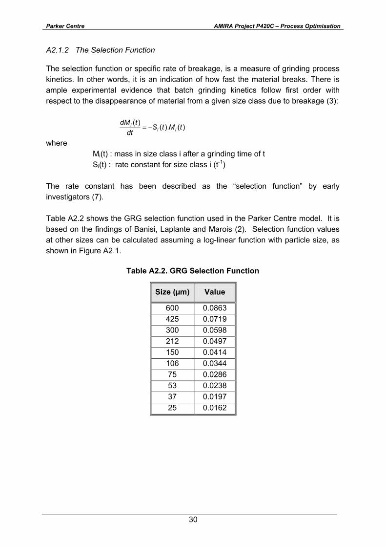
where Mi(t) : mass in size class i after a grinding time of t Si(t) : rate constant for size class i (t-1) The rate constant has been described as the “selection function” by early investigators (7). Table A2.2 shows the GRG selection function used in the Parker Centre model. It is based on the findings of Banisi, Laplante and Marois (2). Selection function values at other sizes can be calculated assuming a log-linear function with particle size, as shown in Figure A2.1.

Table A2.2. GRG Selection Function

Size (µm) Value

600 0.0863 425 0.0719 300 0.0598 212 0.0497 150 0.0414 106 0.0344 75 0.0286 53 0.0238 37 0.0197 25 0.0162


31

0.01

0.1

10 100 1000

Particle Size (µm)

Sele

ctio

n Fu

nctio

n

Figure A2.1. GRG Selection Function

A2.1.3 The Grinding Matrix

The elements Hij in the grinding matrix B, are a function of the breakage and selection functions of the material and the residence time distribution (RTD) in the mill:

Hij = f(Si*τ, bij). For the Parker Centre model, the residence time distribution is assumed to follow a RTD consisting of one plug flow, one large perfect mixer and two small perfect mixers, with 10% in the plug flow, 70% in the large perfect mixer and 10% in each of the two small perfect mixers. The resulting expression is (10):

B =T * [I+Si * τs]–2 * [I+Si * τl]-1 * exp[-Si * τpf] * T-1 Where:

T, T-1 are linear transformation matrices I is the identity matrix τpf, τl, τs are residence time of the plug flow, large and small perfect mixer, respectively.

The tij elements of the matrix T are equal to: tij = 0 if i<j (T is lower triangular...) tij = si if i=j (si are the eigen values...)


32

tSb S-S

1 = t kjkik

1-i

1=kjiij ..∑ if i>j

The aij elements of the matrix T-1 are equal to: aij = 0 if i<j aij = 1/si if i=j

at S1- = a kjik

1-i

1=kiij .∑ if i>j

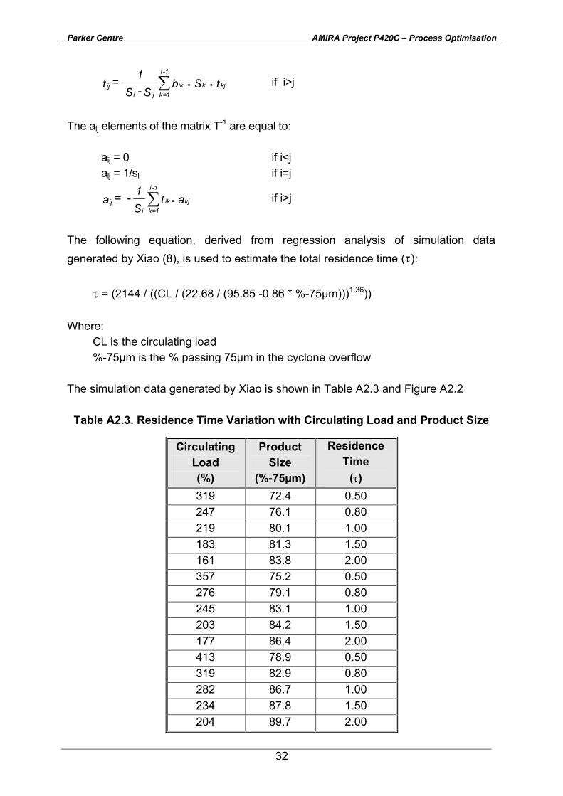
The following equation, derived from regression analysis of simulation data generated by Xiao (8), is used to estimate the total residence time (τ):

τ = (2144 / ((CL / (22.68 / (95.85 -0.86 * %-75µm)))1.36)) Where:

CL is the circulating load %-75µm is the % passing 75µm in the cyclone overflow

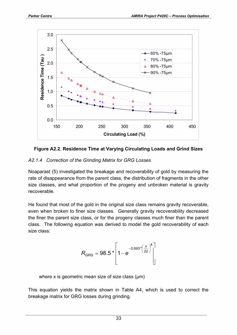
The simulation data generated by Xiao is shown in Table A2.3 and Figure A2.2

Table A2.3. Residence Time Variation with Circulating Load and Product Size

Circulating Load (%)

Product Size

(%-75µm)

Residence Time

(τ) 319 72.4 0.50 247 76.1 0.80 219 80.1 1.00 183 81.3 1.50 161 83.8 2.00 357 75.2 0.50 276 79.1 0.80 245 83.1 1.00 203 84.2 1.50 177 86.4 2.00 413 78.9 0.50 319 82.9 0.80 282 86.7 1.00 234 87.8 1.50 204 89.7 2.00


33

0.0

0.5

1.0

1.5

2.0

2.5

3.0

150 200 250 300 350 400 450

Circulating Load (%)

Res

iden

ce T

ime

(Tau

) 60% -75µm70% -75µm80% -75µm90% -75µm

Figure A2.2. Residence Time at Varying Circulating Loads and Grind Sizes

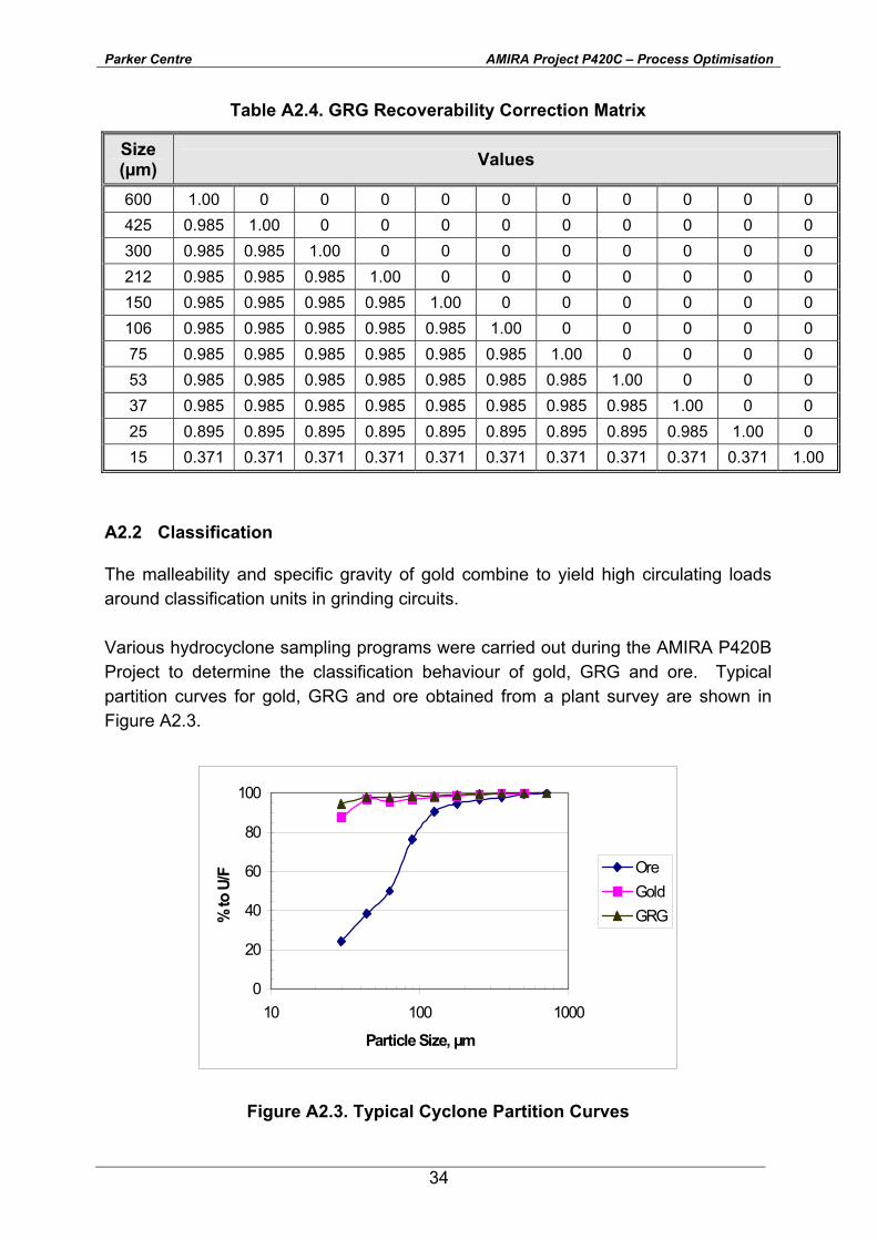
A2.1.4 Correction of the Grinding Matrix for GRG Losses

Noaparast (5) investigated the breakage and recoverability of gold by measuring the rate of disappearance from the parent class, the distribution of fragments in the other size classes, and what proportion of the progeny and unbroken material is gravity recoverable. He found that most of the gold in the original size class remains gravity recoverable, even when broken to finer size classes. Generally gravity recoverability decreased the finer the parent size class, or for the progeny classes much finer than the parent class. The following equation was derived to model the gold recoverability of each size class:

−=

−

4

22*693.0

1*5.98x

GRG eR

where x is geometric mean size of size class (µm)

This equation yields the matrix shown in Table A4, which is used to correct the breakage matrix for GRG losses during grinding.


34

Table A2.4. GRG Recoverability Correction Matrix

Size (µm) Values

600 1.00 0 0 0 0 0 0 0 0 0 0 425 0.985 1.00 0 0 0 0 0 0 0 0 0 300 0.985 0.985 1.00 0 0 0 0 0 0 0 0 212 0.985 0.985 0.985 1.00 0 0 0 0 0 0 0 150 0.985 0.985 0.985 0.985 1.00 0 0 0 0 0 0 106 0.985 0.985 0.985 0.985 0.985 1.00 0 0 0 0 0 75 0.985 0.985 0.985 0.985 0.985 0.985 1.00 0 0 0 0 53 0.985 0.985 0.985 0.985 0.985 0.985 0.985 1.00 0 0 0 37 0.985 0.985 0.985 0.985 0.985 0.985 0.985 0.985 1.00 0 0 25 0.895 0.895 0.895 0.895 0.895 0.895 0.895 0.895 0.985 1.00 0 15 0.371 0.371 0.371 0.371 0.371 0.371 0.371 0.371 0.371 0.371 1.00

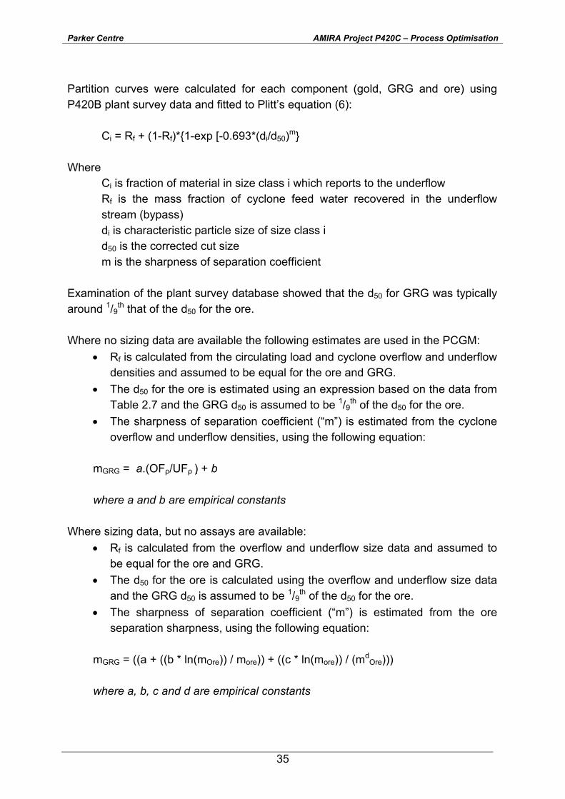
A2.2 Classification

The malleability and specific gravity of gold combine to yield high circulating loads around classification units in grinding circuits. Various hydrocyclone sampling programs were carried out during the AMIRA P420B Project to determine the classification behaviour of gold, GRG and ore. Typical partition curves for gold, GRG and ore obtained from a plant survey are shown in Figure A2.3.

Figure A2.3. Typical Cyclone Partition Curves

0

20

40

60

80

100

10 100 1000

Particle Size, µm

% to

U/F Ore

GoldGRG


35

Partition curves were calculated for each component (gold, GRG and ore) using P420B plant survey data and fitted to Plitt’s equation (6):

Ci = Rf + (1-Rf)*{1-exp [-0.693*(di/d50)m} Where

Ci is fraction of material in size class i which reports to the underflow Rf is the mass fraction of cyclone feed water recovered in the underflow stream (bypass) di is characteristic particle size of size class i d50 is the corrected cut size m is the sharpness of separation coefficient

Examination of the plant survey database showed that the d50 for GRG was typically around 1/9th that of the d50 for the ore. Where no sizing data are available the following estimates are used in the PCGM:

• Rf is calculated from the circulating load and cyclone overflow and underflow densities and assumed to be equal for the ore and GRG.

• The d50 for the ore is estimated using an expression based on the data from Table 2.7 and the GRG d50 is assumed to be 1/9th of the d50 for the ore.

• The sharpness of separation coefficient (“m”) is estimated from the cyclone overflow and underflow densities, using the following equation:

mGRG = a.(OFρ/UFρ ) + b where a and b are empirical constants

Where sizing data, but no assays are available:

• Rf is calculated from the overflow and underflow size data and assumed to be equal for the ore and GRG.

• The d50 for the ore is calculated using the overflow and underflow size data and the GRG d50 is assumed to be 1/9th of the d50 for the ore.

• The sharpness of separation coefficient (“m”) is estimated from the ore separation sharpness, using the following equation:

mGRG = ((a + ((b * ln(mOre)) / more)) + ((c * ln(more)) / (md

Ore))) where a, b, c and d are empirical constants


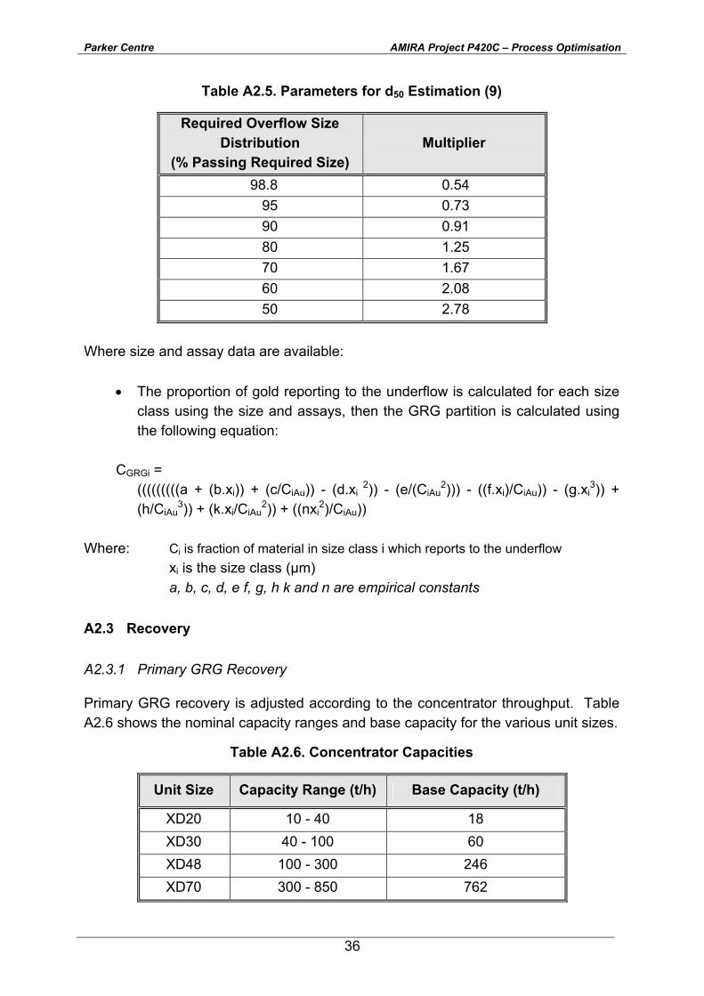
36

Table A2.5. Parameters for d50 Estimation (9)

Required Overflow Size Distribution

(% Passing Required Size) Multiplier

98.8 0.54 95 0.73 90 0.91 80 1.25 70 1.67 60 2.08 50 2.78

Where size and assay data are available:

• The proportion of gold reporting to the underflow is calculated for each size class using the size and assays, then the GRG partition is calculated using the following equation:

CGRGi =

(((((((((a + (b.xi)) + (c/CiAu)) - (d.xi 2)) - (e/(CiAu

2))) - ((f.xi)/CiAu)) - (g.xi3)) +

(h/CiAu3)) + (k.xi/CiAu

2)) + ((nxi2)/CiAu))

Where: Ci is fraction of material in size class i which reports to the underflow

xi is the size class (µm) a, b, c, d, e f, g, h k and n are empirical constants

A2.3 Recovery

A2.3.1 Primary GRG Recovery

Primary GRG recovery is adjusted according to the concentrator throughput. Table A2.6 shows the nominal capacity ranges and base capacity for the various unit sizes.

Table A2.6. Concentrator Capacities

Unit Size Capacity Range (t/h) Base Capacity (t/h)

XD20 10 - 40 18 XD30 40 - 100 60 XD48 100 - 300 246 XD70 300 - 850 762


37

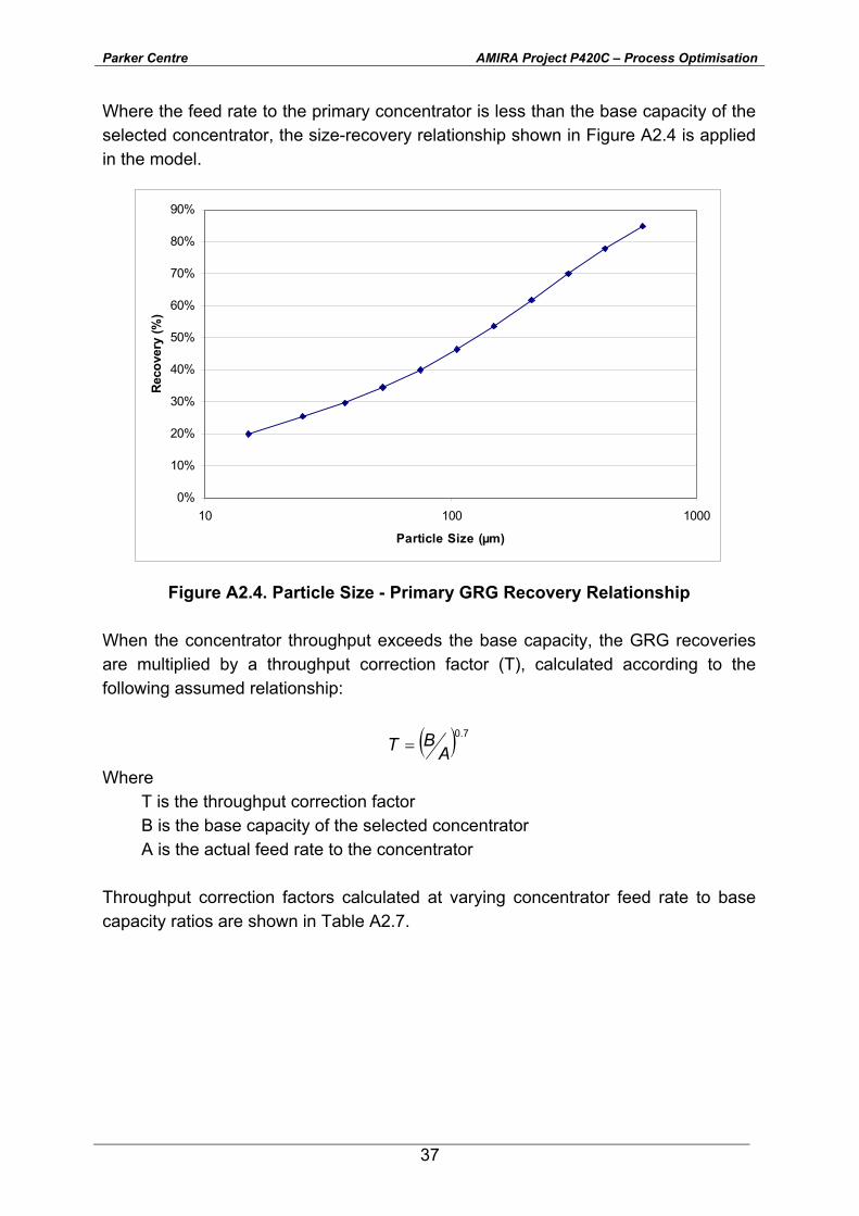
Where the feed rate to the primary concentrator is less than the base capacity of the selected concentrator, the size-recovery relationship shown in Figure A2.4 is applied in the model.

0%

10%

20%

30%

40%

50%

60%

70%

80%

90%

10 100 1000

Particle Size (µm)

Rec

over

y (%

)

Figure A2.4. Particle Size - Primary GRG Recovery Relationship

When the concentrator throughput exceeds the base capacity, the GRG recoveries are multiplied by a throughput correction factor (T), calculated according to the following assumed relationship:

( ) 7.0

ABT =

Where T is the throughput correction factor B is the base capacity of the selected concentrator A is the actual feed rate to the concentrator

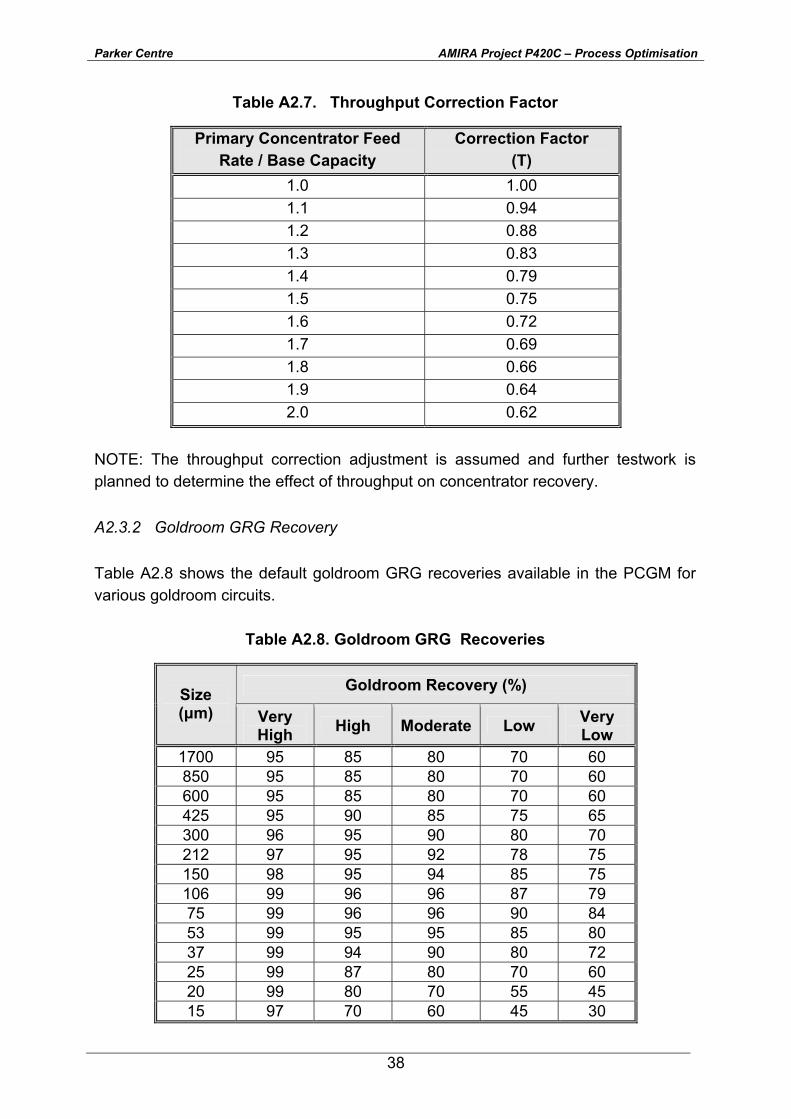
Throughput correction factors calculated at varying concentrator feed rate to base capacity ratios are shown in Table A2.7.


38

Table A2.7. Throughput Correction Factor

Primary Concentrator Feed Rate / Base Capacity

Correction Factor (T)

1.0 1.00 1.1 0.94 1.2 0.88 1.3 0.83 1.4 0.79 1.5 0.75 1.6 0.72 1.7 0.69 1.8 0.66 1.9 0.64 2.0 0.62

NOTE: The throughput correction adjustment is assumed and further testwork is planned to determine the effect of throughput on concentrator recovery.

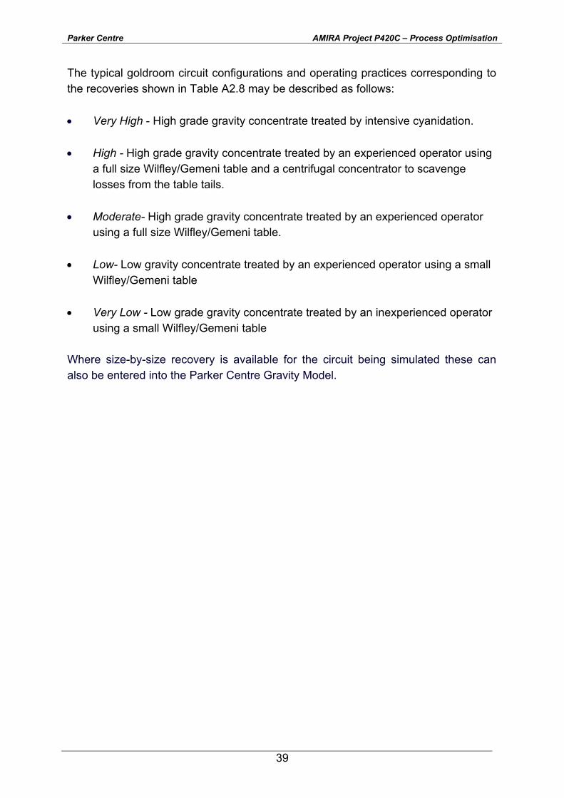
A2.3.2 Goldroom GRG Recovery

Table A2.8 shows the default goldroom GRG recoveries available in the PCGM for various goldroom circuits.

Table A2.8. Goldroom GRG Recoveries

Goldroom Recovery (%) Size (µm) Very

High High Moderate Low Very Low

1700 95 85 80 70 60 850 95 85 80 70 60 600 95 85 80 70 60 425 95 90 85 75 65 300 96 95 90 80 70 212 97 95 92 78 75 150 98 95 94 85 75 106 99 96 96 87 79 75 99 96 96 90 84 53 99 95 95 85 80 37 99 94 90 80 72 25 99 87 80 70 60 20 99 80 70 55 45 15 97 70 60 45 30


39

The typical goldroom circuit configurations and operating practices corresponding to the recoveries shown in Table A2.8 may be described as follows: • Very High - High grade gravity concentrate treated by intensive cyanidation.

• High - High grade gravity concentrate treated by an experienced operator using

a full size Wilfley/Gemeni table and a centrifugal concentrator to scavenge losses from the table tails.

• Moderate- High grade gravity concentrate treated by an experienced operator

using a full size Wilfley/Gemeni table.

• Low- Low gravity concentrate treated by an experienced operator using a small Wilfley/Gemeni table

• Very Low - Low grade gravity concentrate treated by an inexperienced operator

using a small Wilfley/Gemeni table Where size-by-size recovery is available for the circuit being simulated these can also be entered into the Parker Centre Gravity Model.


40

APPENDIX 3 - THE GRG POPULATION BALANCE MODEL

A3.1 Introduction

A methodology to estimate gold recovery by gravity was developed by Laplante et al (1). The method uses a population-balance model (PBM) that represents gold liberation, breakage and classification behaviour to simulate gold gravity recovery in a grinding circuit. This section describes how the PBM is used for GRG characterisation and the description of its behaviour in applicable unit processes. The derivation of the PBM is described, starting from a single class model, progressing to a three-size class model and then to a description of the full size-class model. Typical gravity circuit configurations are presented and matrix equations for calculating the GRG recovery are detailed for each circuit. A3.2 Derivation of the GRG Population Balance Model

A3.2.1 A Simplified Approach

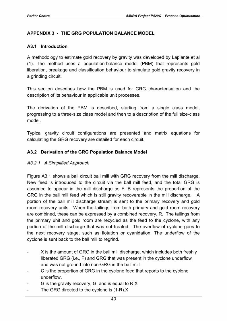
Figure A3.1 shows a ball circuit ball mill with GRG recovery from the mill discharge. New feed is introduced to the circuit via the ball mill feed, and the total GRG is assumed to appear in the mill discharge as F. B represents the proportion of the GRG in the ball mill feed which is still gravity recoverable in the mill discharge. A portion of the ball mill discharge stream is sent to the primary recovery and gold room recovery units. When the tailings from both primary and gold room recovery are combined, these can be expressed by a combined recovery, R. The tailings from the primary unit and gold room are recycled as the feed to the cyclone, with any portion of the mill discharge that was not treated. The overflow of cyclone goes to the next recovery stage, such as flotation or cyanidation. The underflow of the cyclone is sent back to the ball mill to regrind. - X is the amount of GRG in the ball mill discharge, which includes both freshly

liberated GRG (i.e., F) and GRG that was present in the cyclone underflow and was not ground into non-GRG in the ball mill.

- C is the proportion of GRG in the cyclone feed that reports to the cyclone underflow.

- G is the gravity recovery, G, and is equal to R.X - The GRG directed to the cyclone is (1-R).X


41

- The proportion of GRG classified to the underflow of cyclone is C.(1-R).X. - The amount of GRG at the ball mill discharge is the GRG that has “survived”

grinding B.C.(1-R).X , plus an amount F that has been just liberated from the fresh feed, for a total of B.C.(1-R).X + F which is also equal to X:

X= B.C.(1-R).X + F Equation A3.1 Re-arranging equation 3.1 gives,

R)](1*C*B[1

FX−−

= Equation A3.2

or, X = [1-B.C.(1-R)] -1. F And the GRG recovery, G, is equal to:

)]1.(.1[.

RCBFRG−−

= Equation A3.3

This is the simplified PBM derived for this circuit configuration.

B

C

R

Recovery

Fresh Feed X

F

Figure A3.1. GRG Recovery from the Ball Mill Discharge

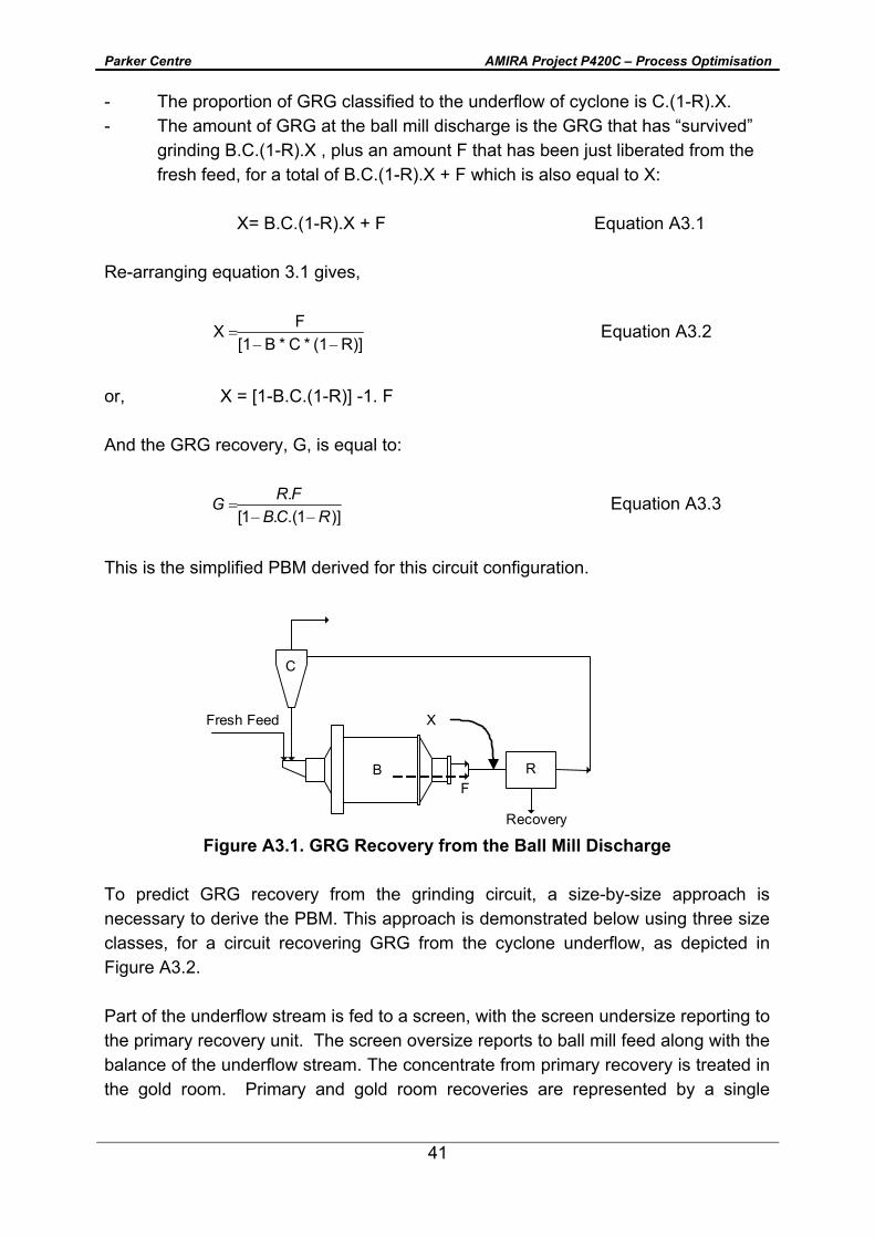
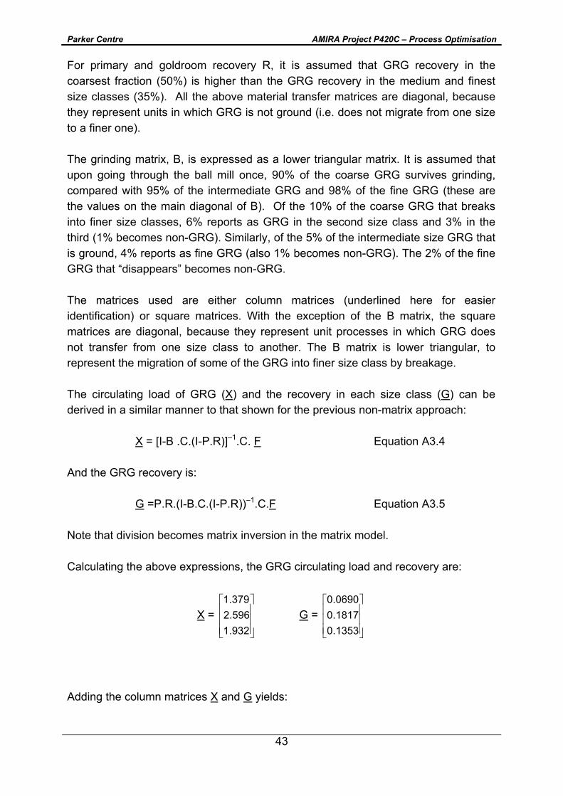
To predict GRG recovery from the grinding circuit, a size-by-size approach is necessary to derive the PBM. This approach is demonstrated below using three size classes, for a circuit recovering GRG from the cyclone underflow, as depicted in Figure A3.2. Part of the underflow stream is fed to a screen, with the screen undersize reporting to the primary recovery unit. The screen oversize reports to ball mill feed along with the balance of the underflow stream. The concentrate from primary recovery is treated in the gold room. Primary and gold room recoveries are represented by a single


42

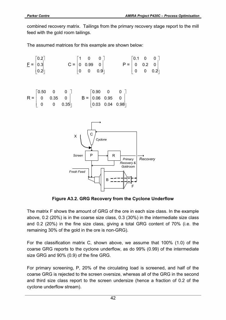
combined recovery matrix. Tailings from the primary recovery stage report to the mill feed with the gold room tailings. The assumed matrices for this example are shown below:

F =

2.03.02.0

C =

9.000099.00001

P =

2.00002.00001.0

R =

35.000035.000050.0

B =

98.004.003.0095.006.00090.0

B

C

P RRecovery

Fresh Feed

X

ScreenPrimary

Recovery & Goldroom

Cyclone

F

Figure A3.2. GRG Recovery from the Cyclone Underflow

The matrix F shows the amount of GRG of the ore in each size class. In the example above, 0.2 (20%) is in the coarse size class, 0.3 (30%) in the intermediate size class and 0.2 (20%) in the fine size class, giving a total GRG content of 70% (i.e. the remaining 30% of the gold in the ore is non-GRG). For the classification matrix C, shown above, we assume that 100% (1.0) of the coarse GRG reports to the cyclone underflow, as do 99% (0.99) of the intermediate size GRG and 90% (0.9) of the fine GRG. For primary screening, P, 20% of the circulating load is screened, and half of the coarse GRG is rejected to the screen oversize, whereas all of the GRG in the second and third size class report to the screen undersize (hence a fraction of 0.2 of the cyclone underflow stream).


43

For primary and goldroom recovery R, it is assumed that GRG recovery in the coarsest fraction (50%) is higher than the GRG recovery in the medium and finest size classes (35%). All the above material transfer matrices are diagonal, because they represent units in which GRG is not ground (i.e. does not migrate from one size to a finer one). The grinding matrix, B, is expressed as a lower triangular matrix. It is assumed that upon going through the ball mill once, 90% of the coarse GRG survives grinding, compared with 95% of the intermediate GRG and 98% of the fine GRG (these are the values on the main diagonal of B). Of the 10% of the coarse GRG that breaks into finer size classes, 6% reports as GRG in the second size class and 3% in the third (1% becomes non-GRG). Similarly, of the 5% of the intermediate size GRG that is ground, 4% reports as fine GRG (also 1% becomes non-GRG). The 2% of the fine GRG that “disappears” becomes non-GRG. The matrices used are either column matrices (underlined here for easier identification) or square matrices. With the exception of the B matrix, the square matrices are diagonal, because they represent unit processes in which GRG does not transfer from one size class to another. The B matrix is lower triangular, to represent the migration of some of the GRG into finer size class by breakage. The circulating load of GRG (X) and the recovery in each size class (G) can be derived in a similar manner to that shown for the previous non-matrix approach: X = [I-B .C.(I-P.R)]–1.C. F Equation A3.4 And the GRG recovery is: G =P.R.(I-B.C.(I-P.R))–1.C.F Equation A3.5 Note that division becomes matrix inversion in the matrix model. Calculating the above expressions, the GRG circulating load and recovery are:

X =

932.1596.2379.1

G =

1353.01817.00690.0

Adding the column matrices X and G yields:


44

- the circulating load of GRG, 5.91 (591%), and - the total gold recovery, 0.3859 (38.6%).

Examination of both matrices shows that the GRG recovery and circulating load are highest in the intermediate size class. This is because the coarsest size class grinds more rapidly and is partially screened out of the gravity circuit feed and the finest size class has a large proportion that reports to the cyclone overflow and its size makes gravity recovery less effective. The circulating load is also highest in the intermediate size class. These trends are typical of actual circuit performance. For the derivation of the above PBM, some assumptions were made. 1. GRG first appears at the discharge of the ball mill with the size distribution

generated by the GRG test, F. 2. No GRG will be rejected to the cyclone overflow before being liberated. The validity of these assumptions was discussed by Laplante et al (1).

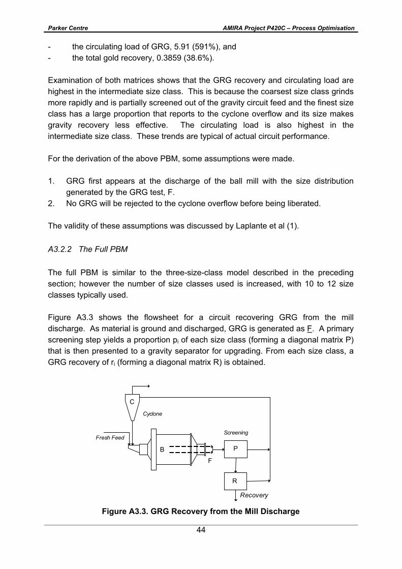
A3.2.2 The Full PBM

The full PBM is similar to the three-size-class model described in the preceding section; however the number of size classes used is increased, with 10 to 12 size classes typically used. Figure A3.3 shows the flowsheet for a circuit recovering GRG from the mill discharge. As material is ground and discharged, GRG is generated as F. A primary screening step yields a proportion pi of each size class (forming a diagonal matrix P) that is then presented to a gravity separator for upgrading. From each size class, a GRG recovery of ri (forming a diagonal matrix R) is obtained.

B

C

P

R

Fresh Feed

Recovery

Screening

Cyclone

F

Figure A3.3. GRG Recovery from the Mill Discharge


45

Material not presented to the gravity circuit combines with the gravity circuit tailings and is then classified by cyclone, a fraction ci (forming a diagonal matrix C) being returned to the mill. In the mill, a fraction of the GRG in each size class remains in the same size class in the mill discharge (the main diagonal of Matrix B), but some GRG reports to finer size classes (the lower triangular submatrix of B). Given the above description, the following formula can be derived in the same manner as that used for the simple PBM:

G = P.R.[I – B.C (I – P.R)]–1.F Equation A3.6 where G is a column matrix of the GRG flowrate into the concentrate for each size class, with the value of gi corresponding to the amount of GRG recovered in size class i. The sum of all the gi values gives the total GRG recovery.

amira project p420c gold processing technology … · amira project p420c gold processing...

Documents