ammonia report 2006-01-20 - ineris.fr · 2.1 physical properties ... conclusion and prospects ......
TRANSCRIPT

Réf. : INERIS - DRA - DRAG – 2005 - 10072 – RBo – AmmoniaPage 1 sur 130
This document forms a non-dissociable entity. It may only be used in its complete form.
WORK STUDY 20/12/2005
N° 10072
AMMONIA
Large-scale atmospheric dispersion tests


Réf. : INERIS - DRA - DRAG – 2005 - 10072 – RBo – AmmoniaPage 1 sur 130
This document forms a non-dissociable entity. It may only be used in its complete form.
AMMONIA
Large-scale atmospheric dispersion tests
INERIS – Accident Risks Division
Translation of the French report:
AMMONIAC : Essais de dispersion d’ammoniac à grande échelle –INERIS-DRA-RBo-1999-20410. R. BOUET

Réf. : INERIS - DRA - DRAG – 2005 - 10072 – RBo – AmmoniaPage 2 sur 130
This document forms a non-dissociable entity. It may only be used in its complete form.
FOREWORD
This report was drawn up on the basis of the information provided to INERIS andthe objective (scientific or technical) data available as well as applicableregulations.
INERIS cannot be held liable if the information received was incomplete orerroneous
Any findings, recommendations, suggestions or equivalent that are recorded byINERIS as part of the services it is contracted to perform may assist with decisionmaking. Given the tasks entrusted to INERIS on the basis of the decree foundingthe organisation, INERIS cannot be involved in the decision making process itself.INERIS cannot therefore take responsibility in lieu and place of the decision-maker.
The addressee shall use the results comprised in this report in whole or at least inan objective manner. Using this information in the form of excerpts or summarymemos may take place only under the full and complete responsibility of theaddressee. The same applies to any modification made to this report.
INERIS declines any liability for any use of this report outside of the scope of theservice provided.
Author Verificateur ApprobateurNAME Rémy BOUET Olivier SALVI Bruno FAUCHER
QualificationProgramme manager
Test activityAccident Risks Division
Scientific manager
Accident Risks Division
Director
Accident Risks Division
Visa Signed Signed Signed

Réf. : INERIS - DRA - DRAG – 2005 - 10072 – RBo – AmmoniaPage 3 sur 130
This document forms a non-dissociable entity. It may only be used in its complete form.
TABLE DES MATIÈRES
1. INTRODUCTION ..............................................................................................7
2. PROPERTIES OF AMMONIA...........................................................................9
2.1 Physical properties........................................................................................9
2.1.1 General points ........................................................................................... 9
2.1.2 Thermodynamic data ................................................................................. 9
2.1.3 Solubility .................................................................................................. 10
2.1.4 Density..................................................................................................... 10
2.2 Explosibility and flammability.......................................................................11
2.2.1 Explosibility limits..................................................................................... 11
2.2.2 Self-ignition temperature.......................................................................... 11
2.2.3 Minimum ignition energy.......................................................................... 11
2.2.4 Extinguishing agents................................................................................ 11
2.3 Reactions with contaminants.......................................................................12
2.3.1 Halogens and inter-halogens................................................................... 12
2.3.2 Heavy metals........................................................................................... 12
2.3.3 Oxidants and peroxides ........................................................................... 12
2.3.4 Acids........................................................................................................ 13
2.3.5 Other aspects .......................................................................................... 13
2.3.6 Stability .................................................................................................... 14
2.4 Toxicity ........................................................................................................14
2.4.1 General.................................................................................................... 14
2.4.2 Acute toxicology....................................................................................... 15
2.4.3 Toxicology at the workplace .................................................................... 16

Réf. : INERIS - DRA - DRAG – 2005 - 10072 – RBo – AmmoniaPage 4 sur 130
This document forms a non-dissociable entity. It may only be used in its complete form.
2.4.4 Summary of results on human toxicology ................................................ 17
2.4.5 Toxicology of fauna and flora................................................................... 20
2.4.5.1 Animals.............................................................................................. 20
2.4.5.2 Aquatic life ......................................................................................... 20
2.4.5.3 Plant life............................................................................................. 21
3. ATMOSPHERIC DISPERSION...................................................................... 23
3.1 Context ....................................................................................................... 23
3.2 Atmospheric dispersion tests...................................................................... 24
3.2.1 Characteristics of accident ammonia releases......................................... 24
3.2.2 Tests by A. Resplandy ............................................................................. 26
3.2.2.1 Context .............................................................................................. 26
3.2.2.2 Test conditions .................................................................................. 27
3.2.2.3 Results .............................................................................................. 29
3.2.3 Tortoise Desert tests................................................................................ 30
3.2.3.1 Context .............................................................................................. 30
3.2.3.2 Test conditions .................................................................................. 31
3.2.3.3 Results .............................................................................................. 32
3.2.4 Unie van Kunstmest Fabrieken bv tests, Netherlands, 1972 ................... 33
3.2.5 Imperial Chemical Industries tests, United Kingdom, 1974...................... 34
3.2.6 Unie van Kunstmest Fabrieken bv tests, Netherlands, 1980 ................... 34
3.2.7 .Landskrona tests, Sweden, 1982............................................................ 35
3.2.8 FLADIS programme tests ........................................................................ 35
3.2.9 Tests conducted at Ecole des Mines, Alès .............................................. 36
3.2.10 Other atmospheric dispersion tests ................................................... 36
3.2.10.1 Summary ........................................................................................... 39
3.3 Modelling of atmospheric ammonia dispersion........................................... 39

Réf. : INERIS - DRA - DRAG – 2005 - 10072 – RBo – AmmoniaPage 5 sur 130
This document forms a non-dissociable entity. It may only be used in its complete form.
3.3.1 Gaussian models ..................................................................................... 40
3.3.2 Three-dimensional models ...................................................................... 40
3.3.3 Integral models ........................................................................................ 40
3.3.4 Residual problems and improvements to be made.................................. 40
3.3.4.1 Two-phase flows ............................................................................... 41
3.3.4.2 Aerosol formation and progression.................................................... 41
3.3.4.3 Pool formation and evaporation......................................................... 41
3.3.5 Summary ................................................................................................. 42
3.4 Issues examined in this programme............................................................43
3.4.1 Impacting jets .......................................................................................... 43
3.4.2 Influence of orifice geometry.................................................................... 44
4. DESCRIPTION OF LARGE-SCALE TESTS ..................................................45
4.1 Presentation of tests conducted ..................................................................45
4.2 Description of test resources.......................................................................47
4.2.1 Description of release point ..................................................................... 47
4.2.2 Weather measurement equipment .......................................................... 52
4.2.3 Ammonia measurement chain composition and tests.............................. 53
4.2.4 Sensor instrumentation on test site ......................................................... 57
4.2.5 Acquisition equipment.............................................................................. 60
4.2.6 Video equipment...................................................................................... 62
4.2.7 Safety ...................................................................................................... 62
5. RELEASE CONDITION MEASUREMENTS...................................................63
5.1 Flow conditions in pipe................................................................................63
5.1.1 Experimental release conditions.............................................................. 63
5.1.2 Release flow condition analyses.............................................................. 67
5.2 Weather conditions during the tests ............................................................73

Réf. : INERIS - DRA - DRAG – 2005 - 10072 – RBo – AmmoniaPage 6 sur 130
This document forms a non-dissociable entity. It may only be used in its complete form.
6. MEASUREMENTS RECORDED LEEWARD FROM RELEASES................. 81
6.1 Ammonia concentration sensors ................................................................ 81
6.2 Analyses..................................................................................................... 88
6.2.1 Influence of release orifice ....................................................................... 89
6.2.2 Influence of atmospheric stability ............................................................. 90
6.2.3 Influence of obstacle placed in near field ................................................. 91
6.2.4 Influence of retention dike........................................................................ 95
6.2.5 Influence of water curtain produced using peacock tail hoses ................. 97
6.2.6 Experiment / modelling comparisons ....................................................... 98
7. CONCLUSION AND PROSPECTS ............................................................. 103
8. BIBLIOGRAPHY.......................................................................................... 105
9. LISTE DES ANNEXES ................................................................................ 111

Réf. : INERIS - DRA - DRAG – 2005 - 10072 – RBo – AmmoniaPage 7 sur 130
This document forms a non-dissociable entity. It may only be used in its complete form.
1. INTRODUCTION
Within the scope of its activities relating to accidental risk, INERIS particularlyneeds to determine safety perimeters around industrial facilities. Following a lossof confinement on a facility, the risks involved may be instantaneous, such as theexplosion of flammable substances, or delayed, such as toxic substance releases.This research programme has concentrated more specifically on the progressionof a toxic cloud formed after an accidental release of pressurised liquid ammoniain storage.
The atmospheric dispersion study on ammonia is of major interest for two reasons.Firstly, ammonia is a widely used substance with a large number of applications,due to its chemical or physical properties. Secondly, ammonia is a highly toxic,corrosive, flammable and explosive substance under certain conditions. Note thatthe loss of confinement of a 22 tonne tank of ammonia on 24 March 1992 in Dakarcaused a large number of deaths (129 deaths and over 1100 injured subjects),some of which occurred several weeks after the accident due to the toxicity ofammonia.
This research programme was essentially financed by the French Ministry forTerritorial Development and the Environment. Six European industrial firms alsocontributed: Norsk Hydro (Norway), Grande Paroisse (France), Veba Oel(Germany), SKW Piesteritz (Germany), CEA-CESTA (France) and Rhône-Poulenc(France). At INERIS, the programme was organised and coordinated in theAccident Risks Division (DRA). It was started in 1995 and completed in 1999.
The main aims of this programme were:
� to analyse the risks represented by facilities using quantities of ammonia ofup to a few dozen tonnes ;
� to complete knowledge on the atmospheric dispersion of ammonia in openand obstructed environments ;
� and to compare the test results with atmospheric dispersion models.
To this end, a large-scale test programme was conducted using a pressurisedliquid ammonia tank. The tests took place on the CEA-CESTA site over a periodfrom December 1996 to April 1997. The purpose of this test campaign was tomeasure the ammonia concentrations leeward from the release in order to obtaina clearer idea on the dispersion of ammonia in the atmosphere in the case ofrealistic releases, particularly in open or semi-obstructed environments.
The best-known pressurised liquefied ammonia dispersion tests are the TortoiseDesert tests conducted by Goldwire et al. (1985) and the FLADIS tests conductedby RISØ (1993/1994). The flow rates used during the Tortoise Desert tests and theFLADIS tests were of the order of 100 kg/s and 0.5 kg/s, respectively. The INERIStests were carried out with intermediary flow rates of the order of 2 to 4 kg/s.

Réf. : INERIS - DRA - DRAG – 2005 - 10072 – RBo – AmmoniaPage 8 sur 130
This document forms a non-dissociable entity. It may only be used in its complete form.
The report is organised as follows. After a description of main properties ofammonia in chapter 2, a summary of atmospheric dispersion in general andammonia dispersion in particular is given in chapter 3. Then, the large-scale testsconducted within the scope of this programme are described in chapter 4. Finally,a summary of the analysis of the release conditions measurements and themeasurements recorded leeward from the releases is given in chapter 5 and 6,respectively.

Réf. : INERIS - DRA - DRAG – 2005 - 10072 – RBo – AmmoniaPage 9 sur 130
This document forms a non-dissociable entity. It may only be used in its complete form.
2. PROPERTIES OF AMMONIA
2.1 PHYSICAL PROPERTIES
This section is particularly based on the Air Liquide (1980), ULMANN (1985) andSNIE (1991) documents
2.1.1 General points
Ammonia is identified as follows (see table 1):
name ammonia
CAS number 7664-41-7
EEC number 007-001-00-5
RTMD hazard code 268
UN number 1005
chemical formula NH3
molar mass 17.03 g
table 1
At atmospheric pressure and 20°C, ammonia is a colourless gas with a pungent,irritant characteristic odour.
2.1.2 Thermodynamic data
The main thermodynamic data for ammonia is as follows:
� Melting point: -77.7°C ;
� Boiling point: -33.4°C to 1.013 bar abs ;
� Variable vapour tension as a function of temperature (see table 2):
Temperature (°C) -77.71 -33.4 -18.7 0 4.7 20 25.7 30 50.1 78.9
Absolutepressure (bar)
0.06077 1.013 2 4.29 5 8.56 10 11.66 20 40
table 2: Vapour tension of ammonia as a function of temperature

Réf. : INERIS - DRA - DRAG – 2005 - 10072 – RBo – AmmoniaPage 10 sur 130
This document forms a non-dissociable entity. It may only be used in its complete form.
� Critical temperature : 405.55 K ;
� Critical pressure : 114.80 bar ;
� Melting heat at 1.013 bar : 332.3 kJ.kg-1 ;
� Vaporisation heat at -15°C: 1210 kJ.kg-1 (289.5 kcal.kg-1) ;
� Vaporisation heat at -33.4°C : 1370 kJ.kg-1 (328 kcal.kg-1) ;
� Dynamic viscosity of liquid at -33.5°C : 10.225 mPa.s.
One litre of liquid releases 947 litres of gas (expanded at 15°C, at a pressure of1 bar).
2.1.3 Solubility
The solubility of ammonia in water is high. Table 3 gives the solubility of ammoniaas a function of temperature (WHO, 1986).
Temperature(°C)
Solubility(g/l)
0 895
20 529
40 316
60 168
table 3: Solubility of ammonia as a function of temperature
In addition, the dissolution of ammonia in water is highly exothermic: 2000 kJ perkilogram of ammonia dissolved in water (i.e. 478.5 kcal.kg-1). As an indication, thedissolution of one kilogram of ammonia releases enough energy to evaporatealmost one and a half kilograms.
2.1.4 Density
� Gas � 0.772 kg.m-3 at 0°C� 0.610 kg.m-3 at 20°C
i.e. a density of 0.597 with reference to air.� Liquid � variable as a function of temperature as indicated in table 4:
Temperature(°C)
-40 -33.4 -20 -10 0 10 15 20 30 50 100 132.4
Density ofliquid ammonia
690 679 659 647 634 621 617 607 592 558 452 235

Réf. : INERIS - DRA - DRAG – 2005 - 10072 – RBo – AmmoniaPage 11 sur 130
This document forms a non-dissociable entity. It may only be used in its complete form.
(kg.m-3)
table 4: Density of ammonia as a function of temperature
2.2 EXPLOSIBILITY AND FLAMMABILITY
The information given below is essentially based on the study conducted byINERIS (Abiven, 1991) at the request of the French Ministry for the Environment.
2.2.1 Explosibility limits
In the literature, different values exist in relation to the Lower and UpperExplosibility Limits (LEL and UEL). The French Ministry for Territorial Developmentand the Environment's Industrial Environment Department data sheet referencedTOX 003-06-1998 gives the following values: LEL 16% and UEL 25%. Thesevalues are also given by INRS (1989) and SAX (1996). Other authors give slightlydifferent values: LEL 15% and UEL 28% according to NFPA (1994) and Medart(1979), LEL 15.5% and UEL 27% according to Weiss (1985).
2.2.2 Self-ignition temperature
The self-ignition temperature of a mixture of gas or vapour is the minimumtemperature from which the mixture is the site of a sufficiently rapid chemicalreaction for a flame to appear spontaneously and propagate throughout themixture. The self-ignition temperature of ammonia recorded in the literature is650°C (Chaineaux, 1991).
2.2.3 Minimum ignition energy
The ignition of a flammable mixture requires the local introduction of a certainquantity of heat. The evaluation of this quantity of energy required to ignite themixture is relatively difficult.
Buckley and Husa (1962) determined the minimum ignition energy of ammoniausing a capacitive system. In this way, they obtained a minimum ignition energy of680 millijoules for ammonia.
Kramer (1985) obtained a minimum energy of 14 millijoules for an ammonia-airmixture. This value, very different to that obtained by Buckley and Husa,demonstrates the difficulty quantifying the release energy of the experimentalsystems used.
However, in spite of this lower value for the minimum ignition energy determinedby Kramer, an air-ammonia mixture has a higher minimum ignition energy (1 to 2orders of magnitude) compared to most air-hydrocarbon mixtures.
2.2.4 Extinguishing agents

Réf. : INERIS - DRA - DRAG – 2005 - 10072 – RBo – AmmoniaPage 12 sur 130
This document forms a non-dissociable entity. It may only be used in its complete form.
The extinguishing agents that must be used consist only of CO2 or powderswhenever there is a possibility of liquid ammonia being present. In fact, if watercomes into contact with liquid ammonia, heat is transmitted to the latter, thusfavouring its vaporisation.
2.3 REACTIONS WITH CONTAMINANTS
Ammonia is used in the manufacture of a large number of nitrous substances.However, hazardous reactions exist with some compounds or families ofcompounds.
The mixture of ammonia with a contaminant may lead to the formation of explosivesubstances.
In its documentary note records (note 1024-84-76), INRS (1976) mentionssubstances inducing hazardous chemical reactions with ammonia, such as nitricacid, oxygen, boron or oxidants
2.3.1 Halogens and inter-halogens
Halogens (fluorine, chlorine, bromine, iodine) react strongly with ammonia and itssolutions. Explosive reactions may also occur with the following substances:acetaldehyde, hypochlorous acid, potassium ferrocyanides. Explosive compoundssuch as nitrogen trihalides are produced.
For example:
� with chlorine, Cl2, mixtures are explosive if they are heated or if chlorine isin excess, due to nitrogen trichloride formation ;
� with bromine pentafluoride, BrF5, explosions are likely.
2.3.2 Heavy metals
Ammonia is capable of reacting with some heavy metals (silver, gold, mercury,etc.), to produce materials liable to explode violently when they are dried:
� with gold chloride (III), AuCl3, under a wide variety of conditions, thepresence of ammonia results in explosive or fulminant compounds whichexplode when heated ;
� with silver oxides, AgO, Ag2O, explosive substances are formed ;
� with mercury, Hg, the reaction gives substances which are highly explosiveand detonate easily. No instrument containing mercury should be used if itis liable to come into contact with ammonia (B.I.T., 1993).
2.3.3 Oxidants and peroxides

Réf. : INERIS - DRA - DRAG – 2005 - 10072 – RBo – AmmoniaPage 13 sur 130
This document forms a non-dissociable entity. It may only be used in its complete form.
Ammonia reacts with a large number of oxides and peroxides: cold chlorineperoxide, hot iodic anhydride, perchlorates, which induce a violent reaction ataround 250°C. The mixture of an oxidant compound and liquefied ammonia isliable to explode under the effect of a shock.
For example:
� with hydrogen peroxide, H2O2, ammonia dissolved in 99.6% of peroxidegives an unstable solution which explodes violently ;
� with nitryl chloride, ClNO2, the interaction is very violent, even at -75°C ;
� with trioxygen difluoride, F2O3, the reaction is liable to cause inflammationsand explosions, even at -183°C. With solid ammonia, it reacts to produceinflammations or explosions;
� with oxygen, O2, if they are placed in contact in a cooling device, anexplosion is liable to occur. In addition, in the presence of ammonia, oxygencan accelerate or induce corrosion.
2.3.4 Acids
With some acids, violent reactions are observed, such as:
� with pure hypochlorous acid, HClO, ammonia, in gaseous form, explodeson contact and releases chlorine;
� with nitric acid, HNO3, an ammonia jet burns in a nitric acid atmosphere
2.3.5 Other aspects
Ammonia can also cause incandescent reactions, for example:
� with boron, B, heated in a dry ammonia atmosphere;
� with chromic anhydride, CrO3, ammonia gas breaks down dry trioxide withincandescence at normal temperatures.
Ammonia can also form self-igniting mixtures:
� with boron, B, heated in a dry ammonia atmosphere;
� with chromic anhydride, CrO3, ammonia gas breaks down dry trioxide withincandescence at normal temperatures.
Ammonia can also form self-igniting mixtures:
� with nitric acid, HNO3, (see section 2.3.4.);

Réf. : INERIS - DRA - DRAG – 2005 - 10072 – RBo – AmmoniaPage 14 sur 130
This document forms a non-dissociable entity. It may only be used in its complete form.
� with chromyl dichloride, CrO2Cl2, ammonia can be ignited with thissubstance.
2.3.6 Stability
At normal temperatures, ammonia gas is a stable compound; its dissociation intohydrogen and nitrogen only starts at around 450 - 500°C. In the presence of somemetals such as iron, nickel, osmium, zinc, uranium, this decomposition starts froma temperature of 300°C and is almost complete at around 500 to 600°C.
2.4 TOXICITY
2.4.1 General
With respect to ammonia toxicity, different published values are available for thesame given effect.
There are three fundamental reasons for this:
� the lack of human testing for high concentrations ;
� the disparity of the subjects making up a human sample, compared to asample of selected laboratory animals for which the response varies verylittle from one animal to another ;
� and the difficulty extrapolating results obtained from animal testing tohumans.
The toxicity of ammonia gas is associated with its very high solubility and thealkalinity of the resulting solutions, rendering it an aggressive agent for mucosaand lungs.
While reliable values on daphnids or rats are available, toxicity on humans is moredifficult to determine. In particular, the influence of the concentration or exposuretime is difficult to assess. With this respect, a study on "acute ammonia toxicity"was conducted by INERIS (Auburtin, 1999).
Exposure to an ammonia-charge atmosphere may induce various types ofphysical effects detailed below:
� Ocular effects: may be induced by the effect of vapours, but also by liquidprojections. They are conveyed by tear production, conjunctivitis liable to beaccompanied by more or less deep corneal effects ;
� Skin effects: in the form of contact dermitis ;

Réf. : INERIS - DRA - DRAG – 2005 - 10072 – RBo – AmmoniaPage 15 sur 130
This document forms a non-dissociable entity. It may only be used in its complete form.
� Respiratory effects: the inhalation of ammonia vapours induces irritation ofthe upper respiratory tract with sneezing, dyspnoea and coughing, the mostsevere stage being acute pulmonary oedema (APO). APO is an accidentwhich occurs following the inhalation of vesicant gases (Cl2, NH3, SO2) bybreaking down the walls of the pulmonary alveoli which are then inundatedwith blood plasma. Fortunately, the olfactory detection threshold ofammonia is well below the concentrations considered to be hazardous ;
� Digestive burns: the ingestion of ammonia is followed by very intensepainful phenomena with gastric intolerance, a state of shock sometimesaccompanied by erythema or purpura. The most dangerous complication isswelling of the glottis.
In direct contact with the skin, liquid ammonia freezes the tissues and causesburns. Ammonia solutions are strongly alkaline and as such highly irritating for themucosa, skin and eyes.
Recurrent long-term exposure to ammonia induces a higher tolerance. Odours andirritants are perceived with more difficulty.
The olfactory perception thresholds are very variable according to the subject,ranging from a few ppm to several dozen ppm.
2.4.2 Acute toxicology
On this point, the results are based on observations made in the case of accidentsand not rigorous experiments; however, the irritation threshold has been measuredon groups of volunteers.
The median lethal concentration (LC501) values, 50 %, are essentially used toevaluate the fatal risks for humans, as it is impossible to conduct suchexperiments on humans.
Data relating to toxicity for humans can only be used if it is associated with:
� a concentration ;
� an exposure time ;
� and a likelihood of effects occurring.
1 LC50: value calculated on the basis of the substance concentration assumed to cause the deathof 50% of the test population for a specified exposure time.

Réf. : INERIS - DRA - DRAG – 2005 - 10072 – RBo – AmmoniaPage 16 sur 130
This document forms a non-dissociable entity. It may only be used in its complete form.
INERIS report (Tissot, 2003) provides the following values:
Time 1 min 3 min 10 min 20 min 30 min 60 min
Lethal Effect Threshold2
(mg/m3)
17 710 10 290 5 740 4 083 3 337 2 380
Irreversible Effect Threshold3
(mg/m3)
1 050 700 606 428 350 248
Odour(mg/m3)
3.62 – 36.2 (i.e. � 5 – 50 ppm)
Note: for ammonia, 1 ppm = 0.70 mg.m-3 and 1 mg.m-3 = 1.43 ppm
table 5: Ammonia toxicity values from INERIS data sheet (Tissot, 2003)
The detection of ammonia by human smell depends on the subject's sensitivity.This olfactory limit is generally from a concentration between 5 and 25 ppm.
This value is well below the threshold corresponding to irreversible damage whichis in turn markedly lower than the threshold for lethal effects. It is important to notethat this aspect is not verified for other gases, such as carbon monoxide, forexample, which is odourless.
2.4.3 Toxicology at the workplace
The authorised concentration for ammonia in working atmospheres is limited andmonitored according to regulations in most industrialised countries. The valuescurrently permitted, which may vary between countries, are generally between 25and 50 ppm. Higher values are defined for short-term exposure or in emergencysituations. The values selected in France are given in table 6 below.
2 Lethal effect threshold: Maximum concentration of pollutant in air at a given exposure time belowwhich, in most subjects, no risk of death is observed.The term "most subjects" excludes "hypersensitive" subjects such as those suffering fromrespiratory failure.
3 Irreversible effect threshold: Maximum concentration of pollutant in air at a given exposure timebelow which, in most subjects, no irreversible effect is observed.An irreversible effect corresponds to the persistence over time of a lesional or functional effectdirectly following exposure in an accidental situation (single and short-term exposure) resultingin incapacitating effects.

Réf. : INERIS - DRA - DRAG – 2005 - 10072 – RBo – AmmoniaPage 17 sur 130
This document forms a non-dissociable entity. It may only be used in its complete form.
Name Definition Value
(ppm)
Observations
TLVC Threshold Limit Value Ceiling at theworkplace for 15 minutes
50 Labour Ministry Circulardated 19 July 1982 France
MLV Mean Limit Value at the workplace for an 8-hour shift
25 Labour Ministry Circulardated 19 July 1982 France
Note: for ammonia, 1 ppm = 0.70 mg.m-3 and 1 mg.m-3 = 1.43 ppm
table 6: Limit values for workplaces in France
2.4.4 Summary of results on human toxicology
The two tables below show different effects observed according to theconcentration and exposure time.
Main results of experimental studies on humans
Concentration
(ppm)
Time
(minutes)
Number ofsubjects
Effects Ref.
Odour
30 8
Perception (sensitive subjects)
Perception
Nuisance
IPCS, 1986
IPCS, 1986
Verbeck, 1977
Unspecified irritation
50
30-50
10
5
6
10
Moderate irritation
Nasal dryness
Mac Ewan, 1972
Report, 1973
Ocular irritation and tear production
130
110-140
150-200
150-200
400
600
700
1000
5
30
360
< 1
30 sec
few sec.
immediate
10
8
6
7
7
7
7
7
Ocular irritation (5 subjects/10)
Nuisance
Tear production, transitory discomfort
Onset of ocular effects (not specified)
Ocular irritation
Tear production
Tear production
Tear production, impaired vision
Report, 1973
Verbeck, 1977
Ferguson, 1977
Wallace, 1978
Wallace, 1978
Wallace, 1978
Wallace, 1978
Wallace, 1978

Réf. : INERIS - DRA - DRAG – 2005 - 10072 – RBo – AmmoniaPage 18 sur 130
This document forms a non-dissociable entity. It may only be used in its complete form.
Respiratory tract irritation and respiratory function disorders
130
150
110-140
500
700
1000
5
8-11
30
30
few sec.
1-3
10
16
8
7
7
7
Throat irritation (8 subjects out of 10)
Respiratory function signs (exercise)
Throat irritation: nuisance
Respiratory tract irritation
Functional signs
Still breathable
Breathing intolerable
Report, 1973
Cole, 1977
Verbeck, 1977
Silverman, 1949
Wallace, 1978
Wallace, 1978
Tolerable / intolerable concentration
140
1500
30-75
instantaneous
8
7
Departure from exposure chamber
Intolerable score for non-experts
Departure from exposure chamber
Verbeck, 1977
Wallace, 1978
table 7: Effects of ammonia on humans
Table 7 is taken from the INERIS study (Auburtin, 1999) on the acute toxicity ofammonia.
As an indication, the NIOSH (1987) proposes an IDLH value (ImmediatelyDangerous to Life or Health) of 500 ppm for ammonia. Note that this IDLH valuecorresponds to a maximum concentration in air up to which a subject exposed fornot more than 30 minutes may escape without risking irreversible effects.

Réf. : INERIS - DRA - DRAG – 2005 - 10072 – RBo – AmmoniaPage 19 sur 130
This document forms a non-dissociable entity. It may only be used in its complete form.
Concentration inmg.m-3
Effects Exposure time
3.5 Perceptible odour for some subjects.
18 Perceptible odour for most subjects. Mean occupational limit value in Franceand in a number of countries
35 - 70 Perceptible irritation for most subjects, inthe eyes.
Tolerable for up to 2 hours for subjectsnot accustomed to exposure;accustomed subjects may toleratehigher concentrations over the sameperiod
87 - 100 Irritation of the eyes, nasal tract andmucosa.
Irritation of the throat and respiratorytract.
Exposure time of over 1 hour.
140 Nausea and headaches.
280 - 490 Immediate irritation of the eyes, nose,throat and upper respiratory tract.
Exposure for ½ hr to 1 hr does not causeserious damage although irritation of theupper respiratory tract may persist for 24hrs following a 30-min exposure period.Aggravation of pre-existing respiratoryproblems may occur.
700 - 1400 Severe coughing. Severe irritation of theeyes, nose and throat, bronchiticspasms.
Damage to the eyes and respiratorysystem may occur if they are not treatedquickly.
A 30-min exposure period may inducevery serious effects on subjects with apredisposition for respiratory problems.
2100 - 2800 Severe coughing. Severe irritation of theeyes, nose and throat.
May be fatal after 30 min.
3500 - 8400 Respiratory spasm. Rapid asphyxia,severe oedema, strangulation.
Fatal in a few minutes.
table 8: Effects on ammonia on humans according to concentration (EFMA-IFA, 1990)
Table 8 is taken from the "guide on risks represented by ammonia" issued bySNIE (1991).

Réf. : INERIS - DRA - DRAG – 2005 - 10072 – RBo – AmmoniaPage 20 sur 130
This document forms a non-dissociable entity. It may only be used in its complete form.
2.4.5 Toxicology of fauna and flora
2.4.5.1 Animals
Table 9 shows some effects observed on animals
Species Concentration inmg.m-3
Effects
75 - 100 Coughing, nasal, oral and lachrymal secretions.Pigs
140 Severe symptoms of irritation and convulsion after 36 hrsof exposure with recovery 7 hrs after end of exposure.
280 A 10-min exposure period induces an irreversiblecessation of ciliary activity.
350 Same effects as above for a 5-min exposure period.
Rabbits
3500 LC 50 – 1 hr.
Cats 3500 LC 50 – 1 hr.
table 9: Toxicological effects of ammonia on some animalsaccording to concentration (EFMA-IFA, 1990)
2.4.5.2 Aquatic life
Free (non-ionised) ammonia in surface water is toxic for fish. However, ammoniumions are not. In this way, in the event of water contamination by ammonia,ammonia salts representing no toxic risk may be formed. The pH value of thewater is important as free ammonia is formed for pH values greater than 7.5-8.0.
For trout, disorders occur from 0.3 mg.l-1. Percidae (or castotomidae) andsalmonidae are the most sensitive varieties for freshwater species. For seawater,prawns appear to be the most sensitive invertebrate species, Depending on thetype of fish, a risk of mortality arises between 1.2 and 5 mg.l-1 (these values referto non-ionised ammonia).
For ionised ammonia (ammonia in solution), lethal concentrations (LC50) for somespecies are given in the table below:
Species Threshold Exposure time Concentration
daphnids LC50 24 hrs 27 mg.l-1
fish LC50 24 hrs 182 mg.l-1

Réf. : INERIS - DRA - DRAG – 2005 - 10072 – RBo – AmmoniaPage 21 sur 130
This document forms a non-dissociable entity. It may only be used in its complete form.
algae LC50 5 days 185 mg.l-1
table 10: lethal concentrations (LC50) for some species
2.4.5.3 Plant life
Ammonia is considered as biodegradable and not accumulable, However, itrequires monitoring in the form of an annual evaluation of water, air and soilreleases for annual uses of over 10 tonnes.
Ammonia can be toxic for some plants as it cannot be excreted. It is assimilated bycombining with carbonate chains, and, in this way, the excess ammonia can passinto the sugar metabolism.
Other plants have functions enabling the assimilation of ammonia thus allowingthem to tolerate ammonia or use it preferentially.


Réf. : INERIS - DRA - DRAG – 2005 - 10072 – RBo – AmmoniaPage 23 sur 130
This document forms a non-dissociable entity. It may only be used in its complete form.
3. ATMOSPHERIC DISPERSION
3.1 CONTEXT
Knowledge of the atmospheric dispersion mechanisms of ammonia is applied inthe following three cases:
� The predictive nature of an atmospheric dispersion study makes it possibleto envisage the potential risks of an industrial facility, particularly within thescope of hazard studies or impact studies ;
� In the event of an accidental situation, modelling the atmospheric dispersionmakes it possible to evaluate the measures to be taken in real time ;
� Following an accident, the analysis of the dispersion conditions in the atmospherecan give a clearer understanding of the causes of these accidents, and in somecases, validate atmospheric dispersion models used for the above mentionedstudies.
There are different approaches to the study of atmospheric dispersion:
� full-scale tests ;
� model (hydraulic or aeraulic) simulation ;
� use of mathematical calculation codes.
The last way to approach gas transportation and diffusion phenomena in theatmosphere offers advantages over the techniques mentioned above such as thefact that complex experimental procedures are not used, the rapid nature of thestudy, and the possibility of envisaging a large number of cases.
However, in order to be able to access simulation, it is necessary to haveextensive knowledge of the phenomena governing atmospheric dispersion. Withthis respect, full-scale tests are required.
Studying the atmospheric dispersion of ammonia is of major interest for tworeasons. Firstly, ammonia is a very toxic, corrosive, flammable and explosivesubstance under certain conditions. Secondly, ammonia is a very widely usedsubstance with numerous applications, due to its chemical or physical properties.
With respect to its chemical properties, the main application of ammonia is themanufacture of fertilisers. Ammonia represents the main concentrated source ofnitrogen for agriculture, which consume approximately 85 to 90% of production.Industry uses ammonia as a raw material for the manufacture of explosives, fibresand plastics. It is also used in the manufacture of paper, rubber, in refineries, theleather industry and the pharmaceutical industry.

Réf. : INERIS - DRA - DRAG – 2005 - 10072 – RBo – AmmoniaPage 24 sur 130
This document forms a non-dissociable entity. It may only be used in its complete form.
With respect to applications associated with physical properties, ammonia is usedas a coolant in compression and absorption systems. Some characteristics ofammonia, such as its high latent heat, its low vapour density and its chemicalstability, favour its use in major industrial facilities.
These two specificities of ammonia, its harmfulness and its widespread userequire, in terms of personal safety, details on its behaviour in the event of loss ofconfinement, particularly in the case of accidental releases into the atmosphere.
Therefore, to this end, this chapter proposes to:
� provide a status report on atmospheric dispersion tests conducted withammonia ;
� present the state of the art and gaps in the knowledge of the modelling ofthe atmospheric dispersion of ammonia, as the modelling of theatmospheric dispersion represents a key stage in the study of toxicsubstance release ;
� and justify the study areas developed within the scope of this researchprogramme.
3.2 ATMOSPHERIC DISPERSION TESTS
After a description of the main characteristics of ammonia releases, this sectionfirst presents atmospheric ammonia dispersion tests and then briefly presentsdispersion tests conducted with heavy gases.
3.2.1 Characteristics of accident ammonia releases
The atmospheric dispersion of a gas is influenced by the release conditions, theweather conditions and also by the type of gas released.
There are different possible types of accidental ammonia releases:
� ammonia gas jet from a pressurised vessel (release from gaseous phase) ;
� two-phase ammonia jet from a pressurised vessel (release from liquidphase) ;
� evaporation of a pool of liquid ammonia in which the temperature is lessthan or equal to its boiling point4 ;
� leakage of liquid ammonia from a cryogenic tank (liquid ammonia at atemperature below the boiling point and at atmospheric pressure).
4 Note that the boiling point of ammonia at normal pressure is -33.4°C.

Réf. : INERIS - DRA - DRAG – 2005 - 10072 – RBo – AmmoniaPage 25 sur 130
This document forms a non-dissociable entity. It may only be used in its complete form.
Ammonia has specific dispersion characteristics and depending on the type ofrelease, the dispersion of the ammonia released will be different. The type ofrelease, which was more specifically studied within the scope of this programme,is the two-phase ammonia release from the liquid phase of a pressurised tank.
All the studies conducted on two-phase releases break down the jet into threemain zones as shown in figure 1 below:
figure 1: two-phase jet
These three main zones are respectively:
� the expansion zone: In this short zone, between 0.5 and 4 times thediameter of the opening (IANELLO, 1989), the fluid is expanded from thepressure at the opening to atmospheric pressure. Due to this suddendepressurisation, the liquid phase of the release is in a superheated stateand a fraction of this liquid phase is vaporised almost instantaneously. Thisphenomenon is known as the "thermodynamic flash". The gaseous phasecreated by this flash phenomenon will have, due to its lower density, ahigher velocity than that of the liquid. This difference in velocity between thetwo phases induces the entrainment of the liquid phase and itsfragmentation into fine droplets. These droplets are entrained by thegaseous phase at a high velocity and form what is referred to as the"aerosol".In this way, at the end of this zone, the jet consists of a gaseous phase anda liquid phase in aerosol form and it is commonly admitted that the entire jet(liquid and gaseous phases) is at the boiling point of the releasedsubstance.
������������
�� ��� ���������� ������������ �������
���� �������

Réf. : INERIS - DRA - DRAG – 2005 - 10072 – RBo – AmmoniaPage 26 sur 130
This document forms a non-dissociable entity. It may only be used in its complete form.
� the entrainment zone: In this zone, the turbulent jet induces theentrainment of the ambient air in the jet. The energy supplied by this airwhich is warmer than the jet is initially used to vaporise the liquid dropletspresent in the jet. This vaporisation cools the jet which then behaves like ajet of heavy gas in the atmosphere.Once the liquid phase has been entirely vaporised, this energy is used toheat the jet which has become entirely gaseous.
� the passive dispersion zone: With the entrainment of air, the velocity ofthe jet progressively decreases until it reaches the wind velocity. From thispoint, the jet is said to be dispersed passively in the atmosphere.
The presence of obstacles is also a factor in the atmospheric dispersion of heavygases, particularly liquefied ammonia.
If the obstacle is sufficiently close to the release, it will modify the initial dispersionphase and subsequently, it will influence the dispersion in the atmosphere. Forexample, a two-phase release in jet form, which encounters an obstacle such as awall or floor, may result in pool formation. In this case, the dispersion of theammonia from the pool is different to that which would have followed the free jet.
On the other hand, if the obstacle is at a distance from the release point, and if thesize of the cloud formed by the ammonia is comparable to the obstacle, theobstacle only modifies the gaseous mass flow and will not modify the physicalstate of the release. In this case, the effect on dispersion will be less than in theprevious case, decreasing according to the dilution and size of the cloud when itencounters the obstacle.
3.2.2 Tests by A. Resplandy
The information contained in this section is based on the A. Resplandy'ssummaries (1967, 1968, 1969).
3.2.2.1 Context
In order to determine the measures to be recommended for the safety of thevicinity of liquefied ammonia storage tanks, A. Resplandy, Official Inspector ofClassified Facilities and Chairman of the Consultative Committee for ClassifiedFacilities, conducted two series of liquid ammonia dispersion experiments. Theytook place, firstly at the Boissise-la-Bertrand army camp in June 1967 and,secondly, at the Mourmelon army camp in March 1968.
The purpose of the experiments was to:
� specify the conditions under which ammonia is diffused into the atmospherefrom a liquid phase spillage in order to determine the radius of the isolationzones to be stipulated around pressurised storage tanks ;
� examine the extent to which refilling of liquid ammonia can be envisaged ;

Réf. : INERIS - DRA - DRAG – 2005 - 10072 – RBo – AmmoniaPage 27 sur 130
This document forms a non-dissociable entity. It may only be used in its complete form.
� test the effectiveness of the intervention resources provided to CivilProtection teams called upon to intervene in the event of an accidentalliquid ammonia leakage.
3.2.2.2 Test conditions
A – Tests at Boissise-la-Bertrand, June 1967
The liquid ammonia tanks consisted of:
� a semi-trailer tanker containing 15 tonnes of ammonia at a pressure of 7bar, equipped with a 2 inch pipe with a flow rate of approximately 20,000kg/hr (5.5 kg/s) in liquid phase and a 1 inch conduit with a flow rate of100 kg of liquid ammonia in approximately 70 seconds (1.4 kg/s) ;
� a tractor-drawn replenishment vehicle comprising two ammonia tanks at 7bar with a unit capacity equal to 2000 kg, each tank being equipped torelease in liquid phase via a 1¼ inch pipe or in gaseous phase via a ¾ inchpipe.
The tests were conducted on 28 June 1967 between 6 am and 11 am. The groundtemperature rose gradually from 13°C to 17°C. The relative humidity wasmaintained in the vicinity of 85%. The wind velocity varied from 0 to 3 m/s.
Two types of measuring device were used:
� 17 Dräger manual detectors:
The Dräger units essentially consisted of a bellows pump used to pass agiven volume of gas through a calibrated tube filled with coloured reagent.Three types of calibrated tubes were used:
� 0.5/a type: sensitivity from 5 to 70 ppm (non-interpretablemeasurements) ;
� 25/a type: sensitivity from 50 to 700 ppm ;
� 0.5%/a type: sensitivity from 0.5 to 10% (non-interpretablemeasurements).
Note that these measuring devices only gave mean values calculated overvariable periods (since the number of pump strokes is not constantaccording to Resplandy) and only allowed a single measurement per test.
� Hartmann and Braun Caldos 2 continuous thermal conductibility analyser:
This unit equipped with a 4-6 mm diameter and 60 m long probe-conduitwas operated coupled with a Philips potentiometric recorder over thefollowing three sensitivity ranges: 0 to 2%, 0 to 4%, 0 to 10%.
Three types of releases were used in order to study:
� the atmospheric diffusion of ammonia from a liquid phase leakage:

Réf. : INERIS - DRA - DRAG – 2005 - 10072 – RBo – AmmoniaPage 28 sur 130
This document forms a non-dissociable entity. It may only be used in its complete form.
� without curtain interposition, using a 2 inch conduit ending with a 90°bend to release vertically upwards, and producing approximately 9releases per minutes, i.e. a released quantity of approximately 330 kg ofliquid ammonia ;
� with curtain interposition, using a 1 inch conduit ending with a 90° bendfitted to a cylindrical vessel in order to be able to guide the jet upwards,as above, or towards the base of the vessel, located 15 cm from the endof the conduit, and performing 2 tests of approximately one minute (onewith an upward jet, the other with a downward jet) ;
� retrievable liquid ammonia refilling possibilities after a storage tankaccident,
� intervention resources in the event of a liquid phase (aerosol) ammonialeakage via the effect of water and heat.
B – Tests at Mourmelon, March 1968
The ammonia was supplied by a 15000 kg semi-trailer tank identical to that for theprevious tests, able to release in liquid phase via a 50 mm diameter pipe, and ingaseous phase via a 30 mm diameter pipe.
The tests were conducted on 28 March 1968 between 8 am and 12:30 pm. Theground temperature rose gradually from 8°C to 18°C. The relative humidity variedfrom 95% to 80%. The wind velocity was between 0 and 3 m/s.
Three recording analysers were used:
� Hartmann and Braun Caldos 2 continuous thermal conductibility analyseridentical to that used above ;
� Kuhlmann conductimetric analyser equipped with a 50 m probe operatingover the 0 to 0.5% range ;
� "ONERA SO" type IR spectrometry analyser equipped with a 50 m probe operatingover the 0 to 0.1% range.
Three types of releases were studied:
� the atmospheric diffusion of ammonia from a liquid phase leakage:
� in the case of a release into a stable atmosphere with a vertical ejection ;
� by varying the orientation of the ejection conduit ;
� by monitoring the progression of the aerosol in terms of stabilised flowrate ;
� by observing the contamination of the atmosphere of a residentialbuilding (caravan) flushed with the ammonia cloud.
� gaseous phase leakage simulation in a pressurised storage tank:

Réf. : INERIS - DRA - DRAG – 2005 - 10072 – RBo – AmmoniaPage 29 sur 130
This document forms a non-dissociable entity. It may only be used in its complete form.
� by varying the direction of ejection ;
� by inserting a curtain during vertical ejection.
� handling of liquid ammonia in the open air:
� by studying the effectiveness of the clay and cement retention dikes ;
� by observing the effect of water on liquid ammonia.
3.2.2.3 Results
In these publications, A. Resplandy (1967, 1968, 1969) gives the following mainresults.
Liquid phase leakages induce the formation of an aerosol, which, beforedissipating, may travel several hundred metres at ground level propelled by thewind. In fact, ammonia's particularly high latent heat of vaporisation only allowsvery slow evaporation of the micro-drops.
The ammonia aerosol is carried by the wind, even if the wind velocity is extremelylow, covering a relatively narrow area, without any diffusion upstream from therelease point. Propagating against the ground, the ammonia droplets may bedeviated from the trajectory given to them by the wind by large obstacles.
An ammonia aerosol is dissipated completely a few minutes after the releasecausing it has stopped and there is no residual hazardous concentration forhumans on the zone covered.
For the same mass of liquid ammonia ejected into the atmosphere from apressurised storage tank, aerosol formation decreases as the temperature of theliquid approaches its boiling point at atmospheric pressure.
In the open air, it is not possible to block the progression of ammonia dropletseffectively with a water spray, even if it is considerable in size.
The relatively rapid diffusion of gaseous ammonia in the atmosphere makes itpossible to envisage, if required, stabilisation by decompressing the contents ofnon-cooled tanks, followed by handling of the stabilised liquid ammonia in theopen air.
Finally, it was demonstrated how dangerous it could be to intervene with water ona sheet of liquid ammonia. In fact, this action results in a significant release of gasand aerosol.
In a liquid phase release from a pressurised ammonia storage tank, by adjustingthe ejection mode (inserting a curtain, direction control), there are limited optionsavailable to reduce aerosol formation and decrease the distance covered by theaerosol front.
Pollution at ground level can be limited by discharging gaseous ammonia verticallyinto the atmosphere from a pressurised tank.

Réf. : INERIS - DRA - DRAG – 2005 - 10072 – RBo – AmmoniaPage 30 sur 130
This document forms a non-dissociable entity. It may only be used in its complete form.
A well-designed system makes it possible to equilibrate the liquid from apressurised tank in the open air by eliminating the vapour phase in theatmosphere.
Liquid phase ammonia equilibrated at atmospheric pressure can be effectivelycollected and stored in the open air in a retention dike; however, the temperaturerise on the casing walls is accompanied by gas and aerosol emission.
The atmospheric dispersion tests conducted by A. Resplandy were among thefirst. They resulted in qualitative observations rather than genuinely interpretablequantitative data. In fact, not many parameters were measured and recorded. Inparticular, there was no precise characterisation of the atmosphere, or precisemeasurements of the ammonia concentration leeward from the release.
These tests particularly made it possible to give ideas on the behaviour ofammonia in the event of an accidental release and outline the perspectives to bestudied. In this way, A. Resplandy proposes three areas of study to complete thestudy conducted:
� specify the influence of the leakage flow rate on the characteristics of theaerosol formed ;
� observe the influence of weather conditions on aerosol characteristics inmore detail ;
� determine the optimal conditions to return pressurised tanks to atmosphericpressure.
3.2.3 Tortoise Desert tests
The releases produced for the Tortoise Desert tests (Goldwire, 1996) were verydifferent to those used by Resplandy.
For example, the quantity of ammonia released on average during the testsconducted by Resplandy in 1967 and 1968 was of the order of 300 to 500 kg witha maximum of 1000 kg for times between 1 and 6 minutes, while for the TortoiseDesert tests, the quantities released were between 10,000 and 41,000 kg.
3.2.3.1 Context
A series of 4 ammonia dispersion tests was conducted during the summer of 1983by the Lawrence Livermore National Laboratory in the United States. These testsare frequently referred to as the Tortoise Desert Tests in the literature. They wereused to study the dispersion of pressurised liquid ammonia releases in theatmosphere.

Réf. : INERIS - DRA - DRAG – 2005 - 10072 – RBo – AmmoniaPage 31 sur 130
This document forms a non-dissociable entity. It may only be used in its complete form.
3.2.3.2 Test conditions
Two tankers with a capacity of 41.5 m3 were used for the tests. Nitrogen tubetrailers were connected to the two tankers in order to maintain the pressure insidethe tankers.
The first test was conducted with a 3.19 inch (81 mm) release orifice and the threeothers were conducted with a 3.72 inch (94.5 mm) diameter orifice. The releasewas horizontal, in the direction of the wind and at a height of 0.79 metres aboveground level.
Table 11 below shows the main characteristics of these releases:
Test Date Releasevolumein m3
Releasemass in
kg
Releasetime in s
Flowrate inkg/s
Windvelocityin m/s
Winddirection
Stabilityclass
1 24/08/83 14.9 10,200 126 81 7.4 224° D
2 29/08/83 43.8 29,900 255 117 5.7 226° D
3 01/09/83 32.4 22,100 166 133 7.4 219° D
4 06/09/83 60.3 41,100 381 109 4.5 220° E
table 11: Characteristics of releases produced during Tortoise Desert tests
Two main devices were used to measure the meteorological data and theconcentrations for the dispersion study.
With respect to the dispersion study, the vapour concentrations were measuredby:
� 20 MSA NDIR gas sensors positioned 100 m from the source and such thatthe gas plus the aerosol passed through a heating device intended tovaporise the aerosol so as to determine the total quantity of NH3 ;
� 31 LLNL IR gas sensors positioned 100 m and 800 m from the source andinitially devised for liquid natural gas (LNG) dispersion tests and notoptimised for ammonia detection, but they made it possible to detectconcentrations above 1% ;
� 24 IST sensors located 0, 800, 1450, 2800 and/or 5500 m from the source.
The data acquisition and storage system used UHF radio waves for datatransmission. All the data acquisition stations and all the stations were portable,battery-operated and gas-tight.

Réf. : INERIS - DRA - DRAG – 2005 - 10072 – RBo – AmmoniaPage 32 sur 130
This document forms a non-dissociable entity. It may only be used in its complete form.
3.2.3.3 Results
The first two tests were conducted on a water-saturated site due to heavy rain.The site was almost completely dry for the third test and completely dry for thefourth, such that the overall weather conditions were more variable than planned.
Test No. 4, the most significant in terms of released quantity, was conductedunder the most stable atmospheric conditions. It demonstrated that the jet wasvisible up to a distance greater than 100 m from the source. The dimensions ofthis cloud, which was heavier than air, are approximately 70 m wide and less than6 m high. The maximum gas concentration observed at 100 m was 6.5%according to Goldwire (1986) and 10% according to Koopman et al (1986). Thecloud had spread over a width of 400 m when it reached 800 m, its height was still6 m. The heavy gas and jet effects dominated the dispersion.
Table 12 below defines some orders of magnitude based on experimental results.It shows maximum concentrations recorded according to the leeward distancefrom the release site.
Distance 100 m 800 m 1450 m 2800 m 5500 m
Maximumconcentration
recorded
6 to 10% 1.4 to 1.6% > 0.5% > 0.5% 100 to200 ppm
table 12: Maximum concentrations observed as a function of leeward distance from the release siteaccording to Koopman et al. (1986) and Goldwire (1985, 1986).
Goldwire et al. (1986) demonstrated the need for "enhanced" simple models topredict the effects of accidental releases. In addition, Hanna et al. (1993) also useGoldwire's results (1985) to compare the results of the models and theexperimental results. The table below gives the concentrations observed on theplume axis.
Tortoise Desert tests 1 2 3 4
Flow rate (kg/s) 81 117 133 109
Concentration at 100 m (ppm) 49,943 83,203 76,881 57,300
Concentration at 800 m (ppm) 8,843 10,804 7,087 16,678
table 13: Concentrations observed on plume axis during Tortoise Desert tests according to Hannaet al. (1993).
These results should be compared to the information contained in table 12.

Réf. : INERIS - DRA - DRAG – 2005 - 10072 – RBo – AmmoniaPage 33 sur 130
This document forms a non-dissociable entity. It may only be used in its complete form.
In relation to these results, several remarks should be noted:
� The highest concentration at 100 m is obtained for test 2 despite a higherflow rate for test 3. The wind velocity for test 2 was lower (5.7 m/s) than fortest 3 (7.4 m/s) and the outdoor temperature was 3°C lower for test 2compared to test 3 ;
� At 800 m, the highest concentration is obtained for test 4, with the lowestflow rate among the releases produced with the 3.72 inch orifice (tests 2, 3,4). On the other hand, the concentration at 100 m was the lowest. Thisresult is explained by most stable weather conditions, stability class Einstead of class D for tests 2 and 3 ;
� Among all the tests, the most unstable weather conditions were recordedduring test 3 (Goldwire, 1985). Under these conditions, in spite of a higherrelease flow rate, the concentration observed on the plume axis at 800 mproves to be the lowest.
These remarks demonstrate that the weather conditions are a very importantfactor in atmospheric dispersion at longer distances, i.e. beyond 100 metres. It isnot sufficient to characterise the source term in detail to model the atmosphericdispersion of ammonia, the weather conditions are also required.
Note: The 4 sections below (§ 3.2.4 to 3.2.7) are essentially based on thedocument produced by Wheatley (April 1987).
3.2.4 Unie van Kunstmest Fabrieken bv tests, Netherlands, 1972
The Unie van Kunstmest Fabrieken bv tests, Netherlands, 1972 were conductedby J. W. Frenken and were reported by Blanken (1980).
The test conditions were as follows:
� vessel containing ammonia at 3.5 bar / 0°C ;
� 8 mm diameter release nozzle ;
� ambient temperature of -10°C ;
� and wind velocity of the order of 2 to 3 m/s.
The purpose of these tests was to measure the quantity of ammonia collected onthe ground in the case of two one-minute releases each releasing 38.4 kg (0.64kg/s) in the following configurations:
� a horizontal release perpendicular to the wind, located 1800 mm fromground level. This release made it possible to collect 5.5 kg of liquidammonia on the ground, i.e. 14.3% of the ammonia released ;

Réf. : INERIS - DRA - DRAG – 2005 - 10072 – RBo – AmmoniaPage 34 sur 130
This document forms a non-dissociable entity. It may only be used in its complete form.
� a vertical release directed towards the ground, 2000 mm from ground level,making it possible to collect 27.3 kg of liquid ammonia on the ground, i.e.71.1% of the ammonia released.
The measurement method for the quantity of ammonia collected is not specified.No measurements of the concentration in the air were made
3.2.5 Imperial Chemical Industries tests, United Kingdom, 1974
The Imperial Chemical Industries tests, United Kingdom, 1974, were reported byReed (1974).
The purpose of the tests was the characterisation of the effectiveness ofpressurised storage tank retention dikes.
Two series of tests were conducted:
� one series intended to simulate the disaster-related rupture of a containerby suddenly removing a lid. The results of these tests are not described byWheatley (April 1987);
� another series of releases via a 1 mm diameter orifice linked by a tube to atank containing ammonia at 6.5 bar/16°C, located 1 m from ground level atvarious angles. When the orifice was horizontal or pointing slightly upwards,an aerosol cloud was formed and no liquid formation was observed on theground. When it was pointing slightly downwards, a small fraction of liquidammonia was collected. The quantity is not specified in Wheatley's report(April 1987).
No other observations were made, and no air concentration measurements weremade.
3.2.6 Unie van Kunstmest Fabrieken bv tests, Netherlands, 1980
The Unie van Kunstmest Fabrieken bv tests, Netherlands, 1980, reported byBlanken (1980), used ammonia stored at 13.4 bar at 38°C and released via a 100mm long and 2 mm diameter capillary tube into moist air.
The purpose of the tests was to study the size of the droplets in the jet. Onlyqualitative results were obtained.
In an ammonia atmosphere, the jet was transparent and the liquid separated fromthe jet and formed a pool on the ground.
In the moist air, the jet was opaque and the liquid ammonia was not collected. Itwas assumed that the ammonia aerosol initially formed was rapidly vaporisedwhen it was diluted with air. In addition, it was concluded that the opacity wascaused by water condensation, which forms an aqueous ammonia aerosol.

Réf. : INERIS - DRA - DRAG – 2005 - 10072 – RBo – AmmoniaPage 35 sur 130
This document forms a non-dissociable entity. It may only be used in its complete form.
No concentration measurements were made.
3.2.7 .Landskrona tests, Sweden, 1982
The Landskrona tests, Sweden, 1982 were conducted by the Swedish NationalDefence Research Institute and were reported by Nyrén et al (1983).
The test conditions were as follows:
� a commercial vessel containing 1400 kg of ammonia at 6 bar and 9°C ;
� an ambient temperature of 8°C and 42% relative humidity ;
� and a wind velocity of 13 m/s.
The purpose of these tests was to measure the flow rate of a two-phase ammoniarelease and compare it to a theoretical model.
The releases were produced from a tube with an internal diameter varyingbetween 32 and 40 mm. Six tests were conducted with a 2 m long tube and fivewith a 3.5 m tube. In each case, the tube was located 2 m above ground level.Each release lasted 60 to 90 s.
For all the tests, except for four, the tank pressure varied considerably. For theremaining four, the outlet pressure was 2.2 bar and the mass flow rate 2.2 kg/s.The jet touched the ground at a point located between 6 and 10 m from therelease point. No pool was observed.
No concentration measurements were made.
3.2.8 FLADIS programme tests
Ammonia releases were produced within the scope of a European test programmecalled FLADIS (Research on the dispersion of two-phase flashing releases). Thisprogramme was conducted under the aegis of DG XII in Brussels (Nielsen & Ott,1996).
Three measurement campaigns were conducted in April and August 1993 and inAugust 1994. In total, 27 horizontal releases of pressurised liquefied ammoniawere produced.
The release flow rates varied from 0.25 to 0.55 kg/s via 4.0 and 6.3 mm diameterorifices. The longest test lasted 40 min.
One of the aims of the FLADIS programme was to study in detail the aerosol jet inthe near field, the heavy gas dispersion phase and the transition from passivedispersion. For this, sensors were positioned in an arc shape centred on therelease point at 20 m, 70 m and 240 m.

Réf. : INERIS - DRA - DRAG – 2005 - 10072 – RBo – AmmoniaPage 36 sur 130
This document forms a non-dissociable entity. It may only be used in its complete form.
Aerosol composition measurements in the two-phase jet were made during thetests. On the basis of these measurements, it was observed that the aerosol,which consisted of almost pure ammonia close to the release point, consisted,within a few meters, of almost pure water.
In addition, no rise in the ammonia cloud was ever observed during the releases.
3.2.9 Tests conducted at Ecole des Mines, Alès
Ecole de Mines, Alès, has conducted several ammonia dispersion test campaignssince 1996. The tests are conducted using one or two 44 kg ammonia cylindersplaced upside down so as to produce liquid phase releases (Bara, Dussere, 1996).The purpose of these tests is to study the effectiveness of the peacock tail hosesused by the fire services.
Downstream from the peacock tail hoses located approximately 1 metre from thecylinders, a reduction in the ammonia concentrations was observed on the releaseaxis, by a factor greater than 10 at a 13 m distance from the cylinders and a factorof at least 3 at a 20 metre distance. On the other hand, no significant reductionwas observed beyond 50 metres.
3.2.10 Other atmospheric dispersion tests
Within the scope of this programme, substance dispersion tests in the atmospherewith gases other than ammonia were taken into consideration.
As mentioned above, ammonia released into the atmosphere generally results inthe formation of a cold cloud, heavier than air. Therefore, dispersion is carried outas for that of a heavy gas until a sufficient level of dilution is reached so that theammonia dispersion is governed solely by the characteristics of the atmosphericflow (passive dispersion).
For this reason, atmospheric dispersion tests conducted on heavy gases are ofinterest for the study of the atmospheric dispersion of ammonia. This is particularlytrue for all aspects relating to the initial release phase.
Table 14 overleaf summarises the main dispersion tests relating to heavy gases.
Note: The Tortoise Desert tests are included in this table for comparison purposes

Réf. : INERIS - DRA - DRAG – 2005 - 10072 – RBo – AmmoniaPage 37 sur 130
This document forms a non-dissociable entity. It may only be used in its complete form.
Burro Coyote TortoiseDesert Goldfish Handford Maplin
SandsPrairieGrass
ThorneyIsland
(instantaneous)
ThorneyIsland
(continuous)
Substance LNG LNG Ammonia Hydrogenfluoride Krypton 85 LNG and
LPGSulphurdioxide
Freon andnitrogen
Freon andnitrogen
Releasetype
Boilingliquid
Boilingliquid
Two-phasereleases
Two-phasereleases Gaseous Boiling
liquid Gaseous jet Gaseous Gaseous
Number oftests 8 3 4 3 5 4 and 8 44 9 2
Quantitiesin kg
10700to
17300
6500to
12700
10000to
36800
3500to
3800
11to
24 Curies
LNG: 2000to 6600
LPG: 1000to 3800
23to63
3150 to
87004800
Time in s 79 to 190 65 to 98 126 to 381 125 to 360 598 to 1191 60 to 360 600 instantaneous 460
Surfacetype
Release onsmall
stretches ofwater
Release onsmall
stretches ofwater
Moist sand Dry lakebed
Desert withbushes
Release onshallow
stretches ofwater
Grass Grass Grass
Stabilityclasses C-E C-D D-E D C-E D A-F D-F E-F
Maximumobservation distance
140 - 800 300 - 400 800 3000 800 400 – 650 800 500 - 580 472
table 14: Summary table of main dispersion tests relating to heavy gases
Note: Thorney Island, 19 tests during phase I; 9 tests during phase II and 3 tests for continuous releases


Réf. : INERIS - DRA - DRAG – 2005 - 10072 – RBo – AmmoniaPage 39 sur 130
This document forms a non-dissociable entity. It may only be used in its complete form.
The study of the tests mentioned in table 14 suggests the following remarks:
� Only the Tortoise Desert and Goldfish tests involved two-phase releases ;
� The liquid release tests on water (Burro, Coyote and Maplin Sands) do notoffer any conclusions for ammonia which has a very different behaviour withwater ;
� Of the tests, only those at Thorney Island used obstacles.
The information obtained from these tests, in terms of dispersion, relates togeneral aspects. Within the scope of these tests, it is not possible to account forthe specificity of ammonia, such as jet formation, aerosol generation, reactionswith air moisture, etc.
3.2.10.1 Summary
The atmospheric dispersion tests already completed have demonstrated:
� the influence of weather conditions ;
� the behaviour of ammonia which is dispersed like a heavy gas when it isreleased from a pressurised tank (no upward dispersion) ;
� a release impacting the ground made it possible to collect 70% of theammonia released (Unie van Kunstmest Fabrieken bv tests, Netherlands,1972).
However, data is particularly lacking on:
� the characterisation of the source term of the release and the formation ofthe two phase jet in the case of pressurised releases and particularlyaerosol generation and progression;
� release tests impacting a surface with higher flow rates. The tests such asthe Unie van Kunstmest Fabrieken bv tests, Netherlands, 1972, did notstudy ammonia dispersion. These tests just studied the phenomenon in aqualitative manner.
3.3 MODELLING OF ATMOSPHERIC AMMONIA DISPERSION
As seen in the previous section, modelling particularly needs to account for:
� gravitational effects due to the cloud temperature ;
� the presence of aerosol ;
� reactions with air moisture.

Réf. : INERIS - DRA - DRAG – 2005 - 10072 – RBo – AmmoniaPage 40 sur 130
This document forms a non-dissociable entity. It may only be used in its complete form.
Different types of dispersion models exist: Gaussian models, integral models andthree-dimensional models. These models are described extensively in theliterature, e.g.: CCPS (1999) or RIOU (1989).
3.3.1 Gaussian models
Purely Gaussian models are, in the majority of cases, unsuitable for the detailedmodelling of pressurised liquid ammonia releases. In fact, ammonia does notbehave like a passive gas in the initial release phases.
3.3.2 Three-dimensional models
Three-dimensional models make it possible to solve the physical equation systemgoverning atmospheric dispersion directly. In this way, a large number of situationsof varying complexity can be simulated. However, this requires preciseincorporation of all phenomena such as, for example, atmospheric turbulence, sitetopography or obstacles.
These models are more complex to implement and require qualified personnel fortheir use. The limitations of these models include the choice of turbulence models,mesh refinement or convergence criteria. For this reason, more simple digitalmodels are used more frequently.
3.3.3 Integral models
Half-way between Gaussian models and three-dimensional models, integralmodels give interesting results with shorter implementation times than three-dimensional models. They make it possible to account for the specificities of thegas and release in the initial phase, until the dispersion becomes passive.
However, such programs do not account for obstacles such as buildings,topography and vegetation. Only a roughness parameter can be used to modulatethe results according to the average site configuration.
3.3.4 Residual problems and improvements to be made
Lantzy (1992) states that it should be borne in mind that the purpose ofatmospheric release modelling is to predict, as accurately as possible, the effectsof a release of hazardous substance. For this purpose, the characterisation of thesource term is decisive, because the best dispersion models will always giveincorrect results if the source term is incorrect.
Some points presented in this article may be repeated for the study of ammoniadispersion, more specifically for the study of the source term for ammoniareleases. These points relate to two-phase flows, aerosol formation andprogression and pool formation and evaporation.

Réf. : INERIS - DRA - DRAG – 2005 - 10072 – RBo – AmmoniaPage 41 sur 130
This document forms a non-dissociable entity. It may only be used in its complete form.
3.3.4.1 Two-phase flows
With respect to two-phase flows, according to Lantzy (1992), future researchshould focus on:
� improved understanding of the effects of non-equilibrium for releases viasmall tubes (less than 100 mm long). This is the scope of interpolationbetween flows in genuine non-equilibrium and homogeneous flows ;
� a more accurate determination of the discharge coefficient. This value isgenerally between 0.6 and 1.0 and, for this reason, has a significantinfluence on the calculated flow rate ;
� the creation of an experimental database for ruptures of pipes with a highL/D ratio. To date, the research carried out in this area has been limited tocomputer simulations. Data is required to verify and extend the existingtheories ;
� the development of entrainment and mixing models for disaster-relatedruptures. For example, there is no entirely satisfactory theory to estimatethe drop size and release velocity correctly. Large-scale data is required tocomplete the small-scale data currently available.
3.3.4.2 Aerosol formation and progression
To model releases from pressurised storage tanks correctly, the models mustaccount for the aerosol and the progression of the droplets along the jet. However,for this, it is necessary to be able to estimate the initial size of drops and theirdistribution accurately. Therefore, most of the research to be developed relates to:
� droplet evaporation. It is necessary to predict the quantity of the substancethat will be transported correctly ;
� droplet coalescence ;
� the effects of viscosity on shearing. No data is available to date ;
� release orifice non-uniformity.
3.3.4.3 Pool formation and evaporation
Pool formation and evaporation is a subject which should be examined in order tounderstand and model the phenomena liable to be encountered during accidents.In particular, the following points must be studied:
� freezing of ground moisture. This phenomenon affects thermal conductiontowards the pool. It is not very clearly understood at the present time ;

Réf. : INERIS - DRA - DRAG – 2005 - 10072 – RBo – AmmoniaPage 42 sur 130
This document forms a non-dissociable entity. It may only be used in its complete form.
� infiltration of substances into the ground. For a cryogenic substance (suchas ammonia), this phenomenon increases the contact surface area whichfavours heat transfer and, for this reason, the evaporation rate. For a non-cryogenic substance, this phenomenon results in a pool with a smallersurface area and less evaporation. As for the above point, this phenomenonis not well known ;
� the effect of the substrate on pool size. There are no good theories linkingthe roughness of the substrate and the pool size directly for a smooth andirregular surface (i.e. in the majority of actual cases) ;
� evaporation with light winds. Data would be required to develop suitablemodels for these conditions.
In addition, with respect to the evaluation of source term models, Lantzy (1992)points out that, generally, the evaluation is not conducted on the source termmodel itself, but on the combination of the source term model and dispersionmodel.
Lantzy also specifies that most of the data available relates to distances of over300 m. Well-designed and well-instrumented tests are required in the vicinity of therelease point so as to compile quality data for the source term model evaluation.
In conclusion, Lantzy expresses the need for satisfactory experimental data for theevaluation and development of all the aspects of source term modelling.
3.3.5 Summary
In sum, a number of technical problems still need to be dealt with in detail invarious areas relating to the study of atmospheric pollutant dispersion.
With respect to source term comprehension and modelling, it is necessary toexamine in detail:
� the two-phase release ;
� pre-mixing in the jet phase ;
� aerosol formation and behaviour in dispersion.
With respect to the specificity of ammonia:
� density ;
� reactions with air moisture.
With respect to the extrinsic conditions for the release:
� definition of weather conditions (wind profile, temperature gradient,hygrometry, etc.) ;

Réf. : INERIS - DRA - DRAG – 2005 - 10072 – RBo – AmmoniaPage 43 sur 130
This document forms a non-dissociable entity. It may only be used in its complete form.
� topography and orography ;
� influence of roughness.
With respect to problems directly associated with modelling:
� limit conditions with the choice of closing equations for three-dimensionalmodels ;
� influence and importance of the different empirical settings for simplifiedmodels and the suitability of these settings with respect to reality ;
� influence of the software user on modelling results.
3.4 ISSUES EXAMINED IN THIS PROGRAMME
This research programme particularly consists of completing knowledge onatmospheric ammonia dispersion in open environments and in obstructedenvironments and making comparisons between results obtained by means ofdigital models and measurements made during tests. To this end, a large-scaletest programme was initiated.
It aims to provide solutions for the problems raised in the previous chapter, morespecifically on the two points presented below.
3.4.1 Impacting jets
Within the scope of an ammonia release study, it is difficult to characterise thesource term correctly, particularly the quantity flowing and forming a liquid pool,referred to as the "rain-out" in the literature.
To try to understand large-scale phenomena, INERIS used ammonia releases inconfigurations differing only by the presence of obstacles in the very near field:
� two-phase jet in open field ;
� two-phase jet impacting a wall at a distance of less than 3 metres ;
� two-phase jet impacting the ground.
The difference between these types of release should make it possible to estimatethe pool formation rate. This potential pool formation in the case of an impactingjet will enable a more realistic approach within the scope of safety studies.

Réf. : INERIS - DRA - DRAG – 2005 - 10072 – RBo – AmmoniaPage 44 sur 130
This document forms a non-dissociable entity. It may only be used in its complete form.
Tests conducted on gaseous jets impacting a surface have demonstrated that,under test conditions, the volume for which the concentration is greater than agiven concentration was much higher than in the case of a free jet, up to 10 timesgreater during tests with methane (Chaineaux, 1995). In fact, when the jet impactsan obstacle, the air entrainment is, in principle, reduced as the cloud tends to be"diluted" with gas-charged air.
If this result is confirmed, it will be necessary to take this aspect into account forsafety in the near field.
However, an impacting jet may result in the formation of a pool on the ground and,therefore, reduce the gas flow rate passing in the atmosphere. The distancescorresponding to a given concentration may then be less than those that would beobtained in the case of an open field release.
Facility safety studies characterised by a configuration similar to these tests will bemore realistic if these phenomena are taken into consideration.
3.4.2 Influence of orifice geometry
Within the scope of the safety studies, releases are generally considered to becircular (due to guillotine pipe rupture).
In this programme, two-phase releases via different orifices, but with the sameopen cross-section surface area, were used, in order to compare the resultsobtained in terms of concentration leeward from the mission.
The reference orifice is a circular orifice (nozzle). Then, an orifice formed by aflange in which the seal was removed beforehand and replaced by blocks of thesame thickness was produced as shown in figure 2 below.
figure 2: Diagram of device used to simulate a leakage on a flange.

Réf. : INERIS - DRA - DRAG – 2005 - 10072 – RBo – AmmoniaPage 45 sur 130
This document forms a non-dissociable entity. It may only be used in its complete form.
4. DESCRIPTION OF LARGE-SCALE TESTS
In this research programme, fifteen large-scale ammonia dispersion tests wereconducted. In order to obtain configurations similar to industrial situations, thetests were defined with the 6 industrial firms taking part in the programme.
4.1 PRESENTATION OF TESTS CONDUCTED
The fifteen release configurations produced during this test campaign are described brieflybelow next to each of the block diagrams. These tests are numbered from 1 to 8 b in thechronological order in which they were carried out. For each of these configurations, thepipe diameter is 2 inch (50.8 mm). Unless specified otherwise (case of tests 2, 3, 4p and2b), the circular orifice also has a diameter of 2 inch.
Horizontal release at a height of 1 metre ingaseous phase. Only test conducted in gasphase. The subsequent tests all relate toammonia releases initially in liquid phase.
Horizontal release at a height of 1 metre inliquid phase via a 20 mm orifice.
Release via a 2 inch flange at a height of 1metre. The distance between the two parts ofthe flange is 1.6 mm such that the releasesurface is equal to 18 mm.
Horizontal release at a height of 1 metre via a30 mm orifice.
Horizontal release at a height of 1 metre.
Horizontal release at a height of 1 metreimpacting a wall with a surface area of 3 m x 3m. This wall is located 3 m from the end of therelease system.
2″1
2″2
20 mm
2″ 3
2″ 4p
30 mm
2″4
2″5

Réf. : INERIS - DRA - DRAG – 2005 - 10072 – RBo – AmmoniaPage 46 sur 130
This document forms a non-dissociable entity. It may only be used in its complete form.
Horizontal release at a height of 1 metreimpacting a wall with a surface area of 3 m x 3m. This wall is located 1 m from the end of therelease system.
Vertical release impacting the ground from aheight of 3 m.
Vertical release impacting the ground from aheight of 1 m.
Vertical release impacting the ground from aheight of 1 m in a retention dike with a surfacearea of 2 m x 2 m and 1 mm high (4 m3).
Release identical to release No. 4. A watercurtain located 25 m from the release point wasstarted up during the test.
Release identical to release No. 4. A watercurtain located 60 m from the release point wasstarted up during the test.
Release identical to No. 4. The temperature ofthe liquid ammonia inside the tank was loweredto -12°C before the test.
Release identical to No. 2 with a 18 mmdiameter orifice.
Vertical release impacting the ground from aheight of 1 m in a retention dike with a surfacearea of 10 m x 10 m and 5 cm high (5 m3).
2″6
2″7
2″8
2″9
2″10
2″11
2″12
2″2b
18 mm
2″8b

Réf. : INERIS - DRA - DRAG – 2005 - 10072 – RBo – AmmoniaPage 47 sur 130
This document forms a non-dissociable entity. It may only be used in its complete form.
4.2 DESCRIPTION OF TEST RESOURCES
To conduct these large-scale ammonia dispersion tests, the CEA-CESTA (Centred'Etudes Scientifiques et Techniques d'Aquitaine, Centre of Scientific andTechnical Studies of Aquitaine) Outdoor Testing Site (TEE) was selected. It islocated approximately sixty kilometres south of Bordeaux. The site covers asurface area of 950 hectares. It is completely enclosed and access to it iscontinuously monitored. The safety study conducted demonstrated that the testsenvisaged could be carried out under satisfactory safety conditions particularly dueto the space available.
The TEE test site is completely flat and free from any obstacles. At the centre ofthis site, which has a radius of approximately two kilometres, there is a squareconcrete slab with 10 metre sides and approximately 15 cm thick. The releaseswere produced from this slab.
4.2.1 Description of release point
In the immediate vicinity of the release slab, three ammonia tanks, of 12 m3 each,were set up. The liquefied ammonia was stored in the tanks at its saturatingvapour pressure. The dimensions of the tanks were as follows:
� total length: 4810 mm
� shell length: 3700 mm
� internal diameter: 1874 mm
� maximum liquid height: 1500 mm
During the tests, only one of these tanks was connected to the release systemlocated at the centre of the slab, which was equipped with 5 thermocouples and apressure sensor, in order to monitor the progression of the pressure andtemperature conditions inside the tank during each test.
The 5 thermocouples were installed on a vertical line from the base of the tank atthe following heights:
� 50 mm
� 400 mm
� 750 mm
� 1100 mm
� 1450 mm
The pressure sensor was located at the top part of the tank, in the gaseous phase.This sensor is referenced P3 in figure 3 overleaf.

Réf. : INERIS - DRA - DRAG – 2005 - 10072 – RBo – AmmoniaPage 48 sur 130
This document forms a non-dissociable entity. It may only be used in its complete form.
The tank was also connected to a nitrogen bundle used either to pressurise it or tokeep the pressure constant during a test, or to purge, after a test, the pipeconnecting it to the release system.
��
����
�� �� ��
��
��
� ����
�!� ��"�#�$��
�%$�&#���!���
�%����!���
'�
� ���# �(��)
�$�����*����
+$�,�����
figure 3: release point diagram
To produce the fifteen releases defined within the scope of this programme, thetwo 2 inch diameter manual valves installed on the tank were used: one wasconnected to the gas phase and the other to the liquid phase. This two identicalvalves are not full bore and their bore diameter is 3/2 inch.
After the 2 inch valve connected to the liquid phase, a 300 mm long and 41 mminternal diameter flow-meter was installed. Intended to operate in liquid phase, itdid not give any interpretable results during the tests as the ammonia was two-phase from the valve located just upstream for almost all the tests.
The connection between the flow-meter and the release system was provided by a50 mm diameter and 10.4 m long pipe.
Finally, the release system consisted of a 2 inch pipe instrumented with valves,thermocouples and pressure sensors (see figure 4 overleaf).

Réf. : INERIS - DRA - DRAG – 2005 - 10072 – RBo – AmmoniaPage 49 sur 130
This document forms a non-dissociable entity. It may only be used in its complete form.
Note: all the distances are given in mm.
figure 4: description of release system
The axis of the release system was located 1015 mm above ground level.
The end of the release system was equipped with different types of outlets (seefigure 5) according to the desired test configuration.
temperature measurement: 1 mm thermocouple at centre of pipeth7
P2
110
280
475
600
715
815
1050
1370
th8 P2 th7
130
445
2" manual valve (3/2” internal diameter)
2" full-bore pneumatic valve
pressure measurement: 15 cm offset sensor
2" diameter10.4 m long
1015
/gro
und
flange (to receivedifferent outlet
types)
release pipe

Réf. : INERIS - DRA - DRAG – 2005 - 10072 – RBo – AmmoniaPage 50 sur 130
This document forms a non-dissociable entity. It may only be used in its complete form.
�!� �� �!�
�!� ��
�!� ��
�!� ��
�!� ��
�!� ��
��
�-�
-�
���
��
���
-��
��
���
���.� �#��
���.� �#��
���
����
����.� �#��
����.� �#��
!� �����$ �$�����/
�����/�0�0��0�0�0��0��0��0�1 �����/ �$�������2$����
����������1
�����/�� ��"�$ �$������!���!��2��
����-/ �$�������������� ����������3�
figure 5: different outlet types for each configuration

Réf. : INERIS - DRA - DRAG – 2005 - 10072 – RBo – AmmoniaPage 51 sur 130
This document forms a non-dissociable entity. It may only be used in its complete form.
For the tests in which the jet was pointing towards the ground, the concrete slabsurface was instrumented with thermocouples. For the jets against the wall, theslab was also instrumented with thermocouples. The instrumentation installed andthe references of the thermocouples are described in appendix 1
photo 1: horizontal release impacting a wall
In the case of tests 2, 4p and 2b, the end of the release system was equipped witha 50 mm pierced cap of a diameter corresponding to the test, i.e. 20 mm, 30 mmand 18 mm for these three tests, respectively.
For test 3 with the flange, the seal was removed. The thickness between the 2parts of the flange was 1.6 mm. This is equivalent to a leakage surface area of 255mm2. Therefore, the equivalent surface diameter is 18 mm.
For tests 10 and 11, water curtains were produced with "peacock tail" hoses. Thecharacteristics of these peacock tails were as follows:
� feed diameter: 70 mm ;� feed pressure: 8 bar ;� water flow rate: 1200 l/min ;� x span: 32 m ;� y span: 10 m.
figure 6: spans of peacock tails used for tests 10 and 11.
�����������
���������� �

Réf. : INERIS - DRA - DRAG – 2005 - 10072 – RBo – AmmoniaPage 52 sur 130
This document forms a non-dissociable entity. It may only be used in its complete form.
For these two tests, two peacock tails were installed as described in figure 7below.
figure 7
Test 10: Layout of both peacock tails 25 mfrom release point.
Test 11: Layout of both peacock tails 60m from release point.
The measurement mast position is specified in detail further in this report.
4.2.2 Weather measurement equipment
To measure the atmospheric conditions, a 10-metre high weather mast was set up350 metres from the release point in the direction noted as 3 (reference M in figure11). It consisted of three vane anemometers, located at a height of 1.5, 4 and 7metres, a weather-cock at 7 metres and an ultrasonic anemometer at 10 metres.
A weather station was also set up next to the control station where thetemperature, relative humidity and solar flux measurements were made. Thesemeasurements were made at a height of 1.5 metres. The acquisition frequency ofthese parameters was 1 Hz, except for the ultrasonic anemometer, which had afrequency of 10 Hz.
4�� 4�� 4��
��
0�
�
��0�
��
0�
�
��� ��� ���
�0
� �0
�
��
��
� ��
�
���"�"3���$
����# �����
����

Réf. : INERIS - DRA - DRAG – 2005 - 10072 – RBo – AmmoniaPage 53 sur 130
This document forms a non-dissociable entity. It may only be used in its complete form.
The type of equipment used is described below:
� 1 PULSONIC 429 weather-cock ;
� 3 PULSONIC 438 vane anemometers ;
� 1 PULSONIC CM6B pyranometer (solar flux measurement) ;
� 1 PULSONIC temperature probe ;
� 1 PULSONIC hygrometer ;
� 1 METEK – USA-1 ultrasonic anemometer.
An installation diagram is given in figure 8 below.
figure 8: Weather mast
The ultrasonic anemometer was installed with the x axis facing north and the yaxis facing east.
The weather-cock was facing the opposite direction to the ultrasonic anemometer.
4.2.3 Ammonia measurement chain composition and tests
To conduct the large-scale tests, INERIS chose to use a standalone measurementchain both to minimise wiring, and also to be easy to move according to weatherconditions (particularly wind direction variations). For this reason, the sensor
10m
7m
4m
1.5m
ultrasonic anemometer
,���!� �"�"3
vane anemometer

Réf. : INERIS - DRA - DRAG – 2005 - 10072 – RBo – AmmoniaPage 54 sur 130
This document forms a non-dissociable entity. It may only be used in its complete form.
electrical power supply was provided by batteries and cells. For each series ofmeasurements, the data was stored on "EEPROM5".
In this way, the ammonia measurement chain consisted of an electronic unit onwhich it was possible to connect up to 4 sensors with different technologies. Intotal, 70 identical electronic units were produced for this programme.
An electronic unit comprises three parts arranged on an assembly plate inside an airtighthousing:
� An electronic signal acquisition card, used to amplify the signal, perform thedigital processing, display various parameters, program the configurationand save data. The main component of the card is a microcontrollerspecially adapted for the instrumentation.
� An EEPROM saving device designed for the primary acquisition of the datafrom the sensors in digital signal form (8192 data items).
� An electrical power supply (cells) to power the electronic circuits
The electronic card is equipped with an internal clock which starts up and shutsdown the system at set times. During this period, the EEPROM saves the sensormeasurements at a predetermined rate. For the tests, a 0.25 Hz frequency wasselected, i.e. one measurement every 4 seconds, which made it possible, in viewof EEPROM capacities, to save for 8 hours. At the end of each day of tests, thedata collected and stored in the EEPROM was copied to a PC hard disk via aspecific interface.
To select the sensors to be installed on the 70 electronic units, the releasesenvisaged in section 4.1 were modelled using atmospheric dispersion software.Some general information was obtained from these simulations:
� In principle, it is not necessary to fit sensors capable of measuringconcentrations above 1% gaseous ammonia beyond 300 metres from therelease point on the plume axis ;
� however, up to 200 metres from the release point, the sensors located onthe plume axis should all be subject to concentrations above 1% ;
� finally, beyond 750 metres, the calculated concentrations are below 0.1%,i.e. 1000 ppm.
These results were considered as orders of magnitude and were adjustedaccording to the progress of the programme.
In this way, the sensors were selected according to the concentration to bemeasured, which is associated with the distance to the release point leeward from
5 EEPROM: Electrically Erasable Programmable Read Only Memory

Réf. : INERIS - DRA - DRAG – 2005 - 10072 – RBo – AmmoniaPage 55 sur 130
This document forms a non-dissociable entity. It may only be used in its complete form.
the emission and the distance to the plume axis.
Several ammonia concentration measurement techniques could be envisaged,such as:
� electrochemical cells ;
� semiconductors ;
� catalytic sensors including pellistors ;
� indirect ammonia measurement by measuring oxygen in the air, based onthe paramagnetic properties of oxygen ;
� measurement in infrared (IR) ;
� chromatography.
Each of these techniques applies to a specific concentration range as shown infigure 9 below. The concentration ranges are orders of magnitude which can beextended according to the characteristics of the sensors.
Logarithmic concentration scale in ppm and %
1 10 100 1000 1 % 10% 100 %
Electrochemical cell
Semiconductor
Catalytic sensor
Indirect O2measurement
Infrared andphotoacousticspectrometry

Réf. : INERIS - DRA - DRAG – 2005 - 10072 – RBo – AmmoniaPage 56 sur 130
This document forms a non-dissociable entity. It may only be used in its complete form.
Chromatography
figure 9: Representation of specific concentration ranges for sensors
Appendix 2 describes the operating principle of the first three techniquesmentioned above, which are the most widely used for combustible gasmeasurements.
Finally, the sensors, which were connected to the electronic units during the testcampaign, are:
� pellistor type catalytic sensors, specific for ammonia (EEV VQ 41) used tomeasure ammonia concentrations between 0.1% and 15% (between 1000ppm and 150,000 ppm). These sensors, 60 in number, were placed in thenear field (up to 200 metres from the release point) ;
� electrochemical cells (SENSORIC NH3 3E 1000) measuring ammoniaconcentrations between 10 and 1000 ppm. These sensors, 50 in number,were arranged in the far field (200 metres to 1700 metres from the releasepoint) ;
� 60 thermocouples (K type, 1 mm diameter, class 1, stainless steel sheath, 5m long), used to measure temperature fluctuations. These thermocoupleswere installed next to each catalytic sensor up to a distance of 100 metresfrom the release point, particularly in order to assess temperature variationsin the jet.
The EEV VQ41 pellistors and the SENSORIC NH3 3E 1000 electrochemical cellsfirst of all underwent a series of laboratory tests at INERIS in order to verify theircharacteristics. The behaviour of these sensors was then tested at INERIS in a 50metre long gallery with a 10 m2 cross-section. Releases via 0.5 mm to 8 mmdiameter orifices were carried out for these tests and made it possible to validatethe measurement chain (Bouet, 1996).
To facilitate data processing, the microcontroller was programmed to supply thedata directly in the unit (ppm vol.) and in the scale corresponding to the sensor.The data was stored in EEPROM as follows:
� electrochemical cell: in 10 ppm intervals up to 2000 ppm ;
� pellistor: in 250 ppm intervals from EEPROM value 0 to 130, and then in560 ppm intervals from EEPROM value 131 to 255 ;
� thermocouple: in 0.3125°C intervals, from -40°C to +40°C.

Réf. : INERIS - DRA - DRAG – 2005 - 10072 – RBo – AmmoniaPage 57 sur 130
This document forms a non-dissociable entity. It may only be used in its complete form.
Finally, a programme used to read and backup the data saved by the EEPROMwas developed based on Labview software. A processing tool for this data wasalso developed based on this software.
4.2.4 Sensor instrumentation on test site
To enable easier installation of the electronic units before a release, the test sitewas also equipped beforehand with 150 x 3 m high masts. These masts offeredthe possibility of attaching the sensors at 4 different heights, i.e. 0.1, 1, 2 and 3metres. They were arranged on 7 arcs 180° in amplitude centred on the releaseslab, with radii of 20, 50, 100, 200, 500, 800 and 1700 metres. On the first twoarcs located at 20 and 50 metres, 41 masts were installed every 4.5°, and on allthe arcs, 21 masts were installed every 9°.
To enable easier subsequent processing of the tests, the masts installed on thetest site were identified by a letter and a number.
photo 2: Masts installed on the tests site
The letter corresponds to the radius of the arc, i.e. the distance from the releasepoint (see table 15).

Réf. : INERIS - DRA - DRAG – 2005 - 10072 – RBo – AmmoniaPage 58 sur 130
This document forms a non-dissociable entity. It may only be used in its complete form.
distance fromrelease point
(m)20 50 100 200 500 800 1700 4 350 650
letter A B C D E F G S M T
table 15: Correspondence between distance from release point and associated letter.
The last three distances of 4, 350 and 650 metres identified in the above tablecorrespond to the sensors installed on the release slab, the weather mast and a19 metre high mast, respectively. In the case of the latter, from test 8, twoelectrochemical cells are installed at heights of 6 and 10 metres.
The number corresponds to a direction from the release point. We defined 80directions, i.e. an angle of 4.5° between each. In the selected configuration, thenorth corresponds to the direction 50 (see figure 10). The layout of the masts wascarried out in the directions between 1 and 41.
The numbering of the angles from the release slab is given in figure 10 below.
figure 10: Identification of angles on release slab
����������������
����������
������
����
��
����
�� �� ��
��
��
�$�����*����
�5��
'6����3�����
����
�����
����
'6����3
'6����3

Réf. : INERIS - DRA - DRAG – 2005 - 10072 – RBo – AmmoniaPage 59 sur 130
This document forms a non-dissociable entity. It may only be used in its complete form.
The numbering of the angles on the test site and the position of the masts aregiven in figure 11 below.
figure 11
Due to the favourable wind direction identified during the initial weather dataanalysis and the test site configuration, the measurement field defined in principlewas located between the directions numbered 1 to 41.
29 (1 680 m)
Release systemControl room
Life zone
G
F
E
D
(1580 m) 1
1113
9
7
5
17
3
15
25 (1 530 m)
23 (1 515 m)
21 (1 540 m)
19 (1 605 m)
41 (1 620 m)
39
37
35
33
31
27 (1 580 m)
Meteorological mast
M
T
CA
B

Réf. : INERIS - DRA - DRAG – 2005 - 10072 – RBo – AmmoniaPage 60 sur 130
This document forms a non-dissociable entity. It may only be used in its complete form.
The arc at 1700 metres is limited by the dimensions of the test site for thedirections 1, 19, 21, 23, 25, 27, 29 and 31. For these directions, the distance atwhich the masts were positioned is given in brackets.
In each test, the sensors were installed on measurement masts in their finalposition leeward from the release approximately 1 hour before the start of the test.In this way, the sensors were all distributed along each side of the release axis onan angular sector ± 35° on either side of the axis.
For the impacting releases and the release via the flange, the sensor distributionangle was greater for the arcs located at 20, 50 and 100 metres (up to 80° oneither side of the release axis). In these configurations, sensors were also addedto the concrete slab over a 4-metre radius.
4.2.5 Acquisition equipment
The data collected during these tests was saved or processed by three separatetypes of acquisition equipment for the following points:
� the electronic units (measurement chain described in section 4.2.3) used forthe acquisition, firstly, of ammonia concentration values using catalyticsensors and electrochemical cells connected to them and, secondly,temperature values measured via thermocouples which were alsoconnected to them ;
� the LabView acquisition system for the weather sensors and for thepressure sensors located on the release point ;
� acquisition system for the thermocouples located on the release point, i.e.the thermocouples arranged in the tank, on the release system and on theground or concrete blocks (acquisition by scanning).
The acquisition system for the data from the weather sensors and the pressuresensors was installed in the control station, in order to monitor the parametersduring the test, at the same time as the acquisition, in particular:
� the pressure in the tank ;
� the pressure at the centre of the release system ;
� the pressure at the release orifice ;
� the wind velocity ;
� and the wind direction.

Réf. : INERIS - DRA - DRAG – 2005 - 10072 – RBo – AmmoniaPage 61 sur 130
This document forms a non-dissociable entity. It may only be used in its complete form.
The location and acquisition frequency for each of these sensors are given in table16 below.
sensorsdistance fromrelease point
(m)�(°) – dir No. z
(m)
acquisitionfrequency
(Hz)
vane anemometer 350 211.5 - 3 7 1
vane anemometer 350 211.5 - 3 4 1
vane anemometer 350 211.5 - 3 1.5 1
ultrasonic anemometer 350 211.5 - 3 10 10
weather-cock 350 211.5 - 3 7 1
tank T (50 mm) release system 0.05 0.2
tank T (400 mm) release system 0.4 0.2
tank T (750 mm) release system 0.75 0.2
tank T (1100 mm) release system 1.1 0.2
tank T (1450 mm) release system 1.45 0.2
pipe T (th8) release system 1 0.2
pipe T (th7) release system 1 0.2
orifice T (th6) release system 1 0.2
thermocouples 11 to 30 Ground and obstacle 0.2
solar flux 450 270 - 70 1.5 1
relative humidity 450 270 - 70 1.5 1
temperature probe 450 270 - 70 1.5 1
ammonia sensors Leeward from releases 0.25
tank pressure (P3) release system 1.9 1
pipe pressure (P2) release system 1 1
orifice pressure (P1) release system 1 1
table 16: sensor position and acquisition frequency

Réf. : INERIS - DRA - DRAG – 2005 - 10072 – RBo – AmmoniaPage 62 sur 130
This document forms a non-dissociable entity. It may only be used in its complete form.
4.2.6 Video equipment
To monitor the tests from the control station, five CEA-CESTA cameras wereplaced on the test site:
� one surveillance camera at a height of 30 metres located between therelease point and the control station ;
� one camera located 10 metres behind the release point, at a height of 10metres ;
� one camera located 40 metres behind the release point, at a height of 26metres ;
� one camera located 1000 metres behind the release point in direction 33, ata height of 1 metre ;
� one mobile camera at a height of 1.5 metre, positioned perpendicular to therelease direction.
4.2.7 Safety
To conduct these tests, the site was divided into four zones:
� the "forefront zone" where the releases were carried out ;
� the "support zone", which was located in a 200 metre radius around therelease point ;
� the "control room", located 450 metres windward from the release point ;
� and the "living zone", located at the entrance to the site approximately 1400metres from the release point.
Each person present on the site was equipped with a filtering mask. In the "controlroom", the personnel present wore "tyvec" clothing. Six people equipped withspecial clothing and an individual breathing apparatus were prepared to intervenein the "support zone". Two of these people were also equipped with a pressuresuit to intervene in the "forefront zone", in particular, if required, in the coldammonia cloud. This never occurred.
No personnel were present to the ammonia release outside the "control room",apart from the six people located in the "support zone".
The different teams working on the site communicated with radio equipment.
A shower system was set up at the entrance to the "forefront zone".
A medical service was available at any times next to the "control room".

Réf. : INERIS - DRA - DRAG – 2005 - 10072 – RBo – AmmoniaPage 63 sur 130
This document forms a non-dissociable entity. It may only be used in its complete form.
5. RELEASE CONDITION MEASUREMENTS
In order to understand the atmospheric dispersion of a pressurised liquefiedammonia release, it is important, firstly, to determine the ammonia flow conditionsin the pipe, and, secondly, to evaluate the weather conditions at the time ofrelease correctly.
5.1 FLOW CONDITIONS IN PIPE
Initially, we will present the experimental conditions in which the releases carriedout within the scope of this programme were conducted. Then, these releaseconditions are analysed.
5.1.1 Experimental release conditions
The experimental conditions under which the tests were conducted are frequentlyreferred to as the "source term" of the release. The source term particularlyspecifies the flow rate, temperature, pressure, velocity and quality6 values at theopening. In this programme, the measured source term values are essentiallytemperature and pressure values, along with the quantity of ammonia released.
During each test, the pressure and temperature conditions were measured andrecorded continuously every second, both in the tank and at different points of thepipe (see chapter 4).
As an illustration, the two graphs in figure 12 below show:
� the typical progression of the pressure conditions in the tank and in the pipeduring a release ;
� the progression of the temperatures located at different heights in the tankand located in the pipe.
6 release quality: a single-constituent two-phase flow is essentially characterised by its quality, i.e.the mass fraction of its vapour phase

Réf. : INERIS - DRA - DRAG – 2005 - 10072 – RBo – AmmoniaPage 64 sur 130
This document forms a non-dissociable entity. It may only be used in its complete form.
These two graphs show the conditions measured and recorded during test 4.
figure 12: Progression of pressure and temperature conditions in tank and in release pipe
����������������������������������� �����!"
(essai 4)
0
1
2
3
4
5
6
7
0 100 200 300 400 500 600 700 800#��� �"
(s)
��������� ���"
����� ���# �
� �2�"�� ���# �
7��3� ���# �
������������������������������������� �����!"
(essai 4)
-50
-40
-30
-20
-10
0
10
20
0 100 200 300 400 500 600 700 800Time(s)
#���������� $"
7���� ��# ������3(������)
7���� ��# ������3(������)
7���� ��# ������3(�����)
�#�$������� ��# �(�!�)7���� ��# ������3(�����)
7���� ��# ������3(����)
7���� ��# �1�2� ��#�$����$��(�!�)
��������� ��# �(�!�)

Réf. : INERIS - DRA - DRAG – 2005 - 10072 – RBo – AmmoniaPage 65 sur 130
This document forms a non-dissociable entity. It may only be used in its complete form.
For test 1, the gaseous release was produced from the vapour pressure inside thetank. The tank was then depressurised and the test was stopped when thepressure had reached approximately 1.8 bar absolute.
With respect to test 2, a 1 bar pressure surge was produced beforehand withnitrogen inside the tank. The nitrogen regulation system then kept this pressureconstant throughout the test.
During test 3, via the flange, no nitrogen pressure surge was producedbeforehand. However, the initial existing pressure in the tank was maintainedthroughout the test by means of nitrogen injection.
For all the subsequent tests, no nitrogen pressure surge was produced before thetest and the pressure was not kept constant throughout the test. In this way, foreach test, a varying pressure drop was observed in the tank according to therelease conditions.
For each test, the behaviour of the pressure and temperature sensors wassubstantially the same. As a general rule, with respect to the values measuredduring the tests, it is possible to note that:
� inside the instrumented tank, the value of the temperature in the gaseousceiling was identical to the temperature of the liquid ammonia from thesecond part of the night. On the other hand, after sunrise, temperaturedifferences between the two phases could be observed. In this way,depending on the outside temperature, the sunlight and tank filling rate, thetemperature of the gas phase sometimes increased more rapidly than thatof the liquid phase. Maximum differences of 10°C between the two phaseswere measured within the scope of this programme ;
� before a release, the value of the pressure in the tank rarely correspondedto the saturating vapour pressure of the liquid ammonia temperature. It wasgenerally between the saturating vapour pressure corresponding to thetemperature of the gaseous ceiling of the tank and the saturating vapourpressure corresponding to the temperature of the liquid ammoniadepending on the time of day, the ambient temperature, the sunlightconditions and the tank filling rate. In some configurations, the differencebetween the pressure in the tank and the saturating vapour pressurecorresponding to the temperature of the liquid ammonia was of the order of1 bar ;
� in the case of a release in which the temperature of the gaseous phase wasinitially greater than the temperature of the liquid phase, a decrease in thetemperature of the gas phase to the temperature of the liquid phase wasconventionally observed. Depending on the initial and ambient conditions,the temperature was liable to fall rapidly after the start of the test, and thenbecame equal to the temperature of the liquid phase ammonia during thetest ;

Réf. : INERIS - DRA - DRAG – 2005 - 10072 – RBo – AmmoniaPage 66 sur 130
This document forms a non-dissociable entity. It may only be used in its complete form.
� the pressure inside the tank, progressing under similar conditions to the gasphase saturating vapour curve, could, therefore, in the same way as thetemperature values, change rapidly during the first minute depending on thetime of day and sunlight conditions ;
� once the first minute of the release had elapsed, the pressure andtemperature conditions inside the tank progressed in a constant and slowermanner for the remainder of the release: drop of 200 to 400 mbar for apressure of the order of 6 bar absolute, and 0.5 to 2°C temperaturedecrease ;
� while the ammonia was flowing in the pipe, a drop in pressure and,therefore, temperature was observed between the tank and the orifice.Typically, for a temperature value of approximately 10°C in the tank, thetemperature at the orifice was approximately -15°C ;
� unlike the conditions in the tank during a test, the pressure and temperatureconditions at the opening changed more significantly: on average, drop inpressure between 0.5 and 1 bar for an initial orifice pressure below 3 barabsolute, and decrease in orifice temperature between 5 and 10°C ;
� the pressure and temperature measurements made at the same point of therelease pipe demonstrated that the pressure was similar to the saturatingvapour pressure corresponding to the temperature measured at this point ;
� after the end of the release, since the valves were closed, the temperatureand pressure values progressed more or less rapidly to their pre-testconditions, except for the pressure and temperature at the orifice. In fact,since the orifice is at atmospheric pressure, the liquid ammonia remainingat the orifice continued to be vaporised by lowering its temperature further.
During the tests, no satisfactory continuous flow rate measurement was made.Only the mean release flow rate value was estimated on the basis of the quantityof ammonia released and the release time.

Réf. : INERIS - DRA - DRAG – 2005 - 10072 – RBo – AmmoniaPage 67 sur 130
This document forms a non-dissociable entity. It may only be used in its complete form.
The general characteristics of all the releases carried out are described in thetable below.
Release characteristics
Test No. Time
(sec)
Quantity released
(kg)
Mean flow rate
(kg/s)
1 460 300 0.65
2 440 1980 4.5
3 540 1400 2.6
4 prel. 660 2380 3.6
4 600 2520 4.2
5 600 2520 4.2
6 600 2520 4.2
7 670 2560 3.8
8 875 3420 3.9
9 605 2370 3.9
10 690 2150 3.1
11 600 1800 3
12 660 2000 3
2b 720 1400 1.95
8b 780 2120 2.7
table 17 General characteristics of release conditions
5.1.2 Release flow condition analyses
When ammonia is stored in the liquid state at its saturating vapour pressure, itsuse generally results in a pressurised liquid flow in a pipe. In the event of a ruptureon this pipe, the flow conditions are modified, with the ammonia changing fromoperating pressure and temperature conditions to conditions corresponding toatmospheric pressure and a temperature below that prior to the rupture.

Réf. : INERIS - DRA - DRAG – 2005 - 10072 – RBo – AmmoniaPage 68 sur 130
This document forms a non-dissociable entity. It may only be used in its complete form.
These new conditions at the opening site must be determined in order to estimatethe characteristics of the release, particularly the mass flow rate, the release rate,the release quality, pressure and temperature. These values form what is referredto as the "source term" of the release. The difficulty establishing the mass flow rateof the release at the opening particularly lies in the evaluation of the flow state inthe pipe, If the liquid ammonia encounters a low pressure wave, it is vaporised.Ammonia is said to undergo a thermodynamic flash generating a mixture of liquidand vapour which affects the flow.
A distinction is essentially made between three different flow states, i.e.:
� bubble state: the liquid phase is continuous and contains gas bubbles ; inthis case, liquid is in the majority ;
� annular or semi-annular state: the gas velocity is greater than that of theliquid against the walls of the pipe ;
� dispersed flow: the gas flow rate is high, the liquid is dispersed in the gasphase; in this case, the liquid is the minority phase in the mixture.
In order to determine the source term at the release point, it is necessary tounderstand and determine the characteristics of the flow in the pipe.
There are a large number of models used to describe the release in the case ofejection via a conduit. These models, mentioned for example by Langard (1995),Bigot (1996), U.I.C. (1987), can be classified into three categories in order ofincreasing complexity:
� homogenous equilibrium models (HEM) ;
� models with differences in velocity (between gaseous phase and liquidphase) ;
� non-equilibrium models.
In the homogeneous equilibrium models, the gas and liquid phases are assumedto:
� have the same velocity;
� be distributed homogeneously;
� be at the saturation temperature.
These assumptions imply that:
� the two-phase flow is considered as a homogeneous fluid with averageproperties between those of the gas and liquid ;
� the flow is at thermodynamic equilibrium (no heat or mass exchange takesplace between the phases).

Réf. : INERIS - DRA - DRAG – 2005 - 10072 – RBo – AmmoniaPage 69 sur 130
This document forms a non-dissociable entity. It may only be used in its complete form.
In addition, the flow is assumed to be stationary and one-dimensional.
There are two main categories of equilibrium models:
� isentropic expansion models: in this case, the entropy of the fluid subject tothe expansion remains constant while its enthalpy decreases. In this case,the loss of enthalpy is assumed to be balanced by the gain in kinetic energyin the flow.
� isenthalpic expansion models: in this case, the enthalpy of the fluid remainsconstant while its entropy decreases. This loss is balanced by the frictionenergy applied by the flow.
Van den Akker et al (1983) demonstrated that these two assumptions are equallyunrealistic but that the error generated in the "constant enthalpy" assumption isless significant.
The purpose of these models is to determine the flow rate at the opening. Withinthe scope of this programme, the tests conducted make it possible to determinethe temperature and pressure at the opening and the mean flow rate throughoutthe test. A HEM model makes it possible to determine, in addition to these values,the quality of the flow at the opening. This parameter was not measured directlyduring the tests. A complete model, proposed by Wheatley (April 1987) andbelonging to the HEM model category, is presented below and its results arecompared to the experimental results obtained during the tests.
Modelling of flow rate at opening: Wheatley approach (April 1987)
The purpose of this modelling is to determine on the basis of the tank conditions(Pint, Tint):
� the pressure-temperature conditions at the opening ;
� the mass flow rate of the release ;
� the quality at the opening.
The basic hypotheses for this model are that:
� the fluid expansion is considered to be isentropic and stationary
� the two-phase fluid is considered to be homogenous and in liquid-vapourequilibrium
In this way, the model proposed is based on the following equations:
� entropy equation: Cpliq.Ln(Tint) = Cpliq.Ln(Tb) + 1
1
7
)7(8�9� (1)

Réf. : INERIS - DRA - DRAG – 2005 - 10072 – RBo – AmmoniaPage 70 sur 130
This document forms a non-dissociable entity. It may only be used in its complete form.
� Euler's equation: ��
�
�
��
�
�+= �
����
�1
�����
�
!9���9��
:1 α (2)
� internal pressure equation as a function of temperature and liquid level:
Pint = Psat(T) + �liq.g.hint = ��
���
� −7
�4��� �� + �liq.g.hint (3)
� Specific volume equation: v = (1 – x).vliq + x.vgas (4)
� Clausius-Clapeyron's equation: Lv(T) T(vgas - vliq) �7
����� (5)
After integration, Euler's equation is expressed as follows:
��
�
�
��
�
�+���
����
�−−+−= ���
1
���1$�&1���$�&
$�&
1�����
�
!9�7
78�979;�)77(;�
��
�
:1
ρα (6)
This expression is used to determine the velocity of the fluid at the opening as afunction of the difference in pressure between the tank and the outlet. Since thefluid is assumed to be at saturation, the temperatures are known once thepressures are known.
The coefficient �p is an empirical corrective factor used to account for the effects offriction; as a general rule, it is taken to be equal to 0.6 in the case of a wallopening and equal to 0.8 or 0.9 in the case of a pipe rupture.
The problem then consists of determining the pressure of the fluid at the opening.The existence of a pressure gradient between the tank and the opening induces asignificant acceleration of the fluid, i.e. potential energy is converted into kineticenergy. The velocity of the fluid at the outlet will be limited by the propagation rateof the pressure waves in the fluid, i.e. the speed of sound.
It is accepted that, if the pressure gradient is sufficiently high, the fluid will reachthe speed of sound at the outlet (May, 1996). If this is the case, the flow is said tobe critical.
A critical (or sonic or blocked) single-phase flow is characterised in that adownstream decrease in pressure, below a certain threshold, has no influence onthe flow. This pressure threshold is referred to as the "critical pressure". It isachieved in a well-defined section of the conduit, generally at the outlet. In thissection, the flow rate is equal to the speed of sound in the fluid, so much so thatdisturbances generated downstream do not affect the upstream flow.
Experience shows a similar phenomenon for two-phase flows. On the other hand,it is more difficult to determine the value of the pressure wave propagation rate ina two-phase fluid given that these waves do not move at the same speed in eachof the two phases. However, the experiments conducted for the two-phase flowstudy demonstrated that the speed of sound of a two-phase flow is markedly lower

Réf. : INERIS - DRA - DRAG – 2005 - 10072 – RBo – AmmoniaPage 71 sur 130
This document forms a non-dissociable entity. It may only be used in its complete form.
than the speed of sound of a single-phase flow (Delhaye, 1981). As a result, thecritical flow is achieved more easily in the case of a two-phase flow (May, 1996).
The modelling of the flow rate at the opening using the method proposed byWheatley (April 1997) assumes that the two-phase flow is critical which isequivalent to considering that the velocity of the fluid at the outlet, Ub, is equal tothe speed of sound in the two-phase fluid of quality xb.
Due to the flow isentropy hypothesis, the speed of sound can be obtained usingthe equation:
"�<
��#��
�:
=∂∂=ρ
(7)
In the case of a two-phase fluid, integration at constant entropy is relativelycomplex. Finally, it was demonstrated that the speed of sound is expressed asfollows:
��
�
�
��
�
����
����
����
����
�++
=
1
���
1
�1$�&11
�1��#��
7
78�9�
7
��79;�79
�9�:
ρ
(8)
The density of the fluid at the opening, �b, is obtained using the flowing equation:
1�
�1$�&
1
���
$�&1 �9�
79;�7
78�
�����
����
�
+=ρρ
(9)
In this case, the pressure Pb such that Ub = Usound (equations 6 and 8) is soughtusing an iterative process. Once this pressure is obtained, the release temperatureis known (saturation) and the quality at the opening is determined usingequation 4:
$�&���
$�&11 ��
��
�
ρρ
ρρ
+
+= (10)
The mass flow rate, Gb, is then determined using the conventional equations:
Gb = �b.Ab.Ub (11)
where Ab is the opening surface area
The release pressure value found by testing the equality between the releasevelocity and the speed of sound will determine the type of release. In fact, if thisvalue is above atmospheric pressure, the flow will be critical and the jet willaccelerate further after the opening due to its expansion to atmospheric pressure.

Réf. : INERIS - DRA - DRAG – 2005 - 10072 – RBo – AmmoniaPage 72 sur 130
This document forms a non-dissociable entity. It may only be used in its complete form.
On the other hand, if the pressure obtained is below atmospheric pressure, it hasno physical significance. In this case, the flow will not be critical (the fluid at theopening does not reach the speed of sound) and the pressure at the opening isconsidered to be equal to the atmospheric pressure.
Non-equilibrium models
Models closer to reality exist, referred to as "non-equilibrium models". They makeit possible to account for thermodynamic differences existing with liquid-vapourequilibrium.
In addition, they include the fact that the two phases are separate, and areconsidered separately, i.e. that they can have different velocities and that phasechanges may be limited by heat transfers or accelerated by the presence ofirregularities.
An example includes the "frozen" model which makes the simple assumption thatthere is no change of phase. The flow is then modelled using Bernoulli's equation.
The actual separate phase model evaluates the material, energy and quantity ofmovement on each of the two phases and applies a vaporisation law in view of theflow state. This model is based on empirical correlations qualifying the flow states.
More comprehensive models such as Yan's model (1991), which modelsnucleation, also exist. It particularly makes it possible to estimate the frequency ofoccurrence of bubbles and the progression of their size.
In order to compare the experimental values to theoretical values, two models(Fauske and Wheatley) were used on the basis of the test conditions for the testsconducted by INERIS and described in chapter 4 above. As a general rule, theresults obtained using these models differ substantially from the values recordedduring the tests, where the values obtained using the models were generallygreater than the experimental values.
These results confirm the fact that the modelling of the flow rate in the case of atwo-phase flow is highly complex and that simplified models are unable to accountfor all the phenomena arising during flow. In addition, within the scope of thesetests, which were not intended to study the flow rate at the opening in an in-depthway, but simply to determine it, the release system used consisted of significantpressure drops on a pipe over 12 metres in length.
We verified experimentally that the fluid at the orifice was indeed under saturationconditions, i.e. that the (Tb,Pb) pairs measured experimentally corresponded to the(Tb,Psat(Tb)) pairs, the basic hypothesis for HEM models.

Réf. : INERIS - DRA - DRAG – 2005 - 10072 – RBo – AmmoniaPage 73 sur 130
This document forms a non-dissociable entity. It may only be used in its complete form.
In conclusion, these models are suitable for tank leakages or releases after a shortpipe. They do not account for pressure drops and, therefore, ammoniavaporisation during its transport outside. If an opening is considered to be flushwith the tank wall, ammonia is vaporised instantaneously into the atmospherewithout passing via the three flow states (bubble state, annular state anddispersed flow).
In the tests conducted, the pipe is sufficiently large for the flow to pass via thesethree flow states. In the literature, it is admitted that dispersed flow is establishedwhen the condition L>2D is met (L pipe length, D pipe diameter), which is thecase. In this way, the dynamic behaviour of ammonia is influenced by these threestates and the phenomena are complex to model.
5.2 WEATHER CONDITIONS DURING THE TESTS
The weather conditions are described using a number of parameters, the mainone being associated with the wind velocity, on one hand, and atmosphericturbulence, on the other.
For each test, the atmospheric conditions were recorded using the equipmentdescribed in chapter 4 above. During the recording period, some values measuredwere subject to little and slow variation. This particularly applied to the ambienttemperature, relative humidity and solar flux. Note that these values weremeasured on the weather station next to the control station.
However, other values, such as the wind velocity and direction measured on theweather mast referenced M in figure 11, could be very variable during therecording period.
In order to give an order of magnitude of the weather conditions during the tests,the mean values associated with each of the releases are given in the table below.
Mean atmospheric conditions
Test No.Sheltered
temperatureRelativehumidity
Solar flux(kW/m2)
Wind velocityat height of
7 m
Winddirection at
height of 7 m
1 14°C 76% 0.2 5 m/s 260°
2 8.5°C 84% 0.1 3 m/s 305°
3 5°C 90% 0.04 2.5 m/s 5°
4p 10°C 61% 0.5 3 m/s 10°
4 12.5°C 82% 0.25 3 m/s 290°
5 20°C 50% 0.65 3.5 m/s 310°
6 12°C 75% 0.5 5 m/s 285°
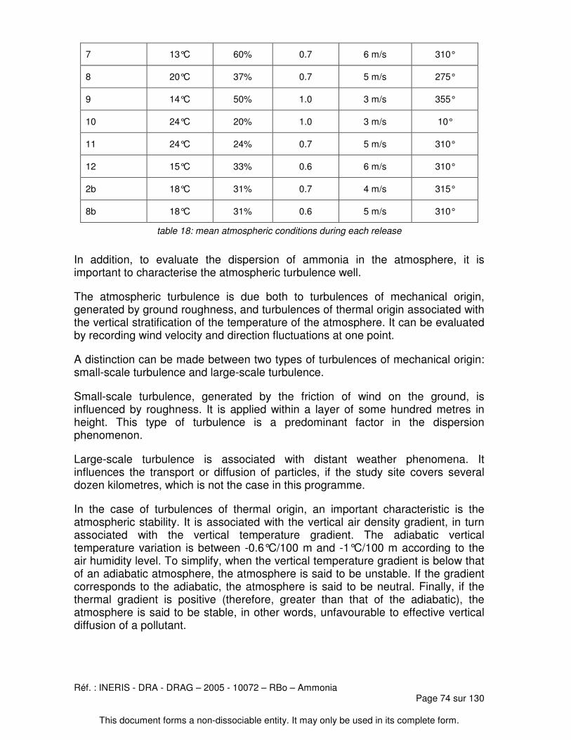
Réf. : INERIS - DRA - DRAG – 2005 - 10072 – RBo – AmmoniaPage 74 sur 130
This document forms a non-dissociable entity. It may only be used in its complete form.
7 13°C 60% 0.7 6 m/s 310°
8 20°C 37% 0.7 5 m/s 275°
9 14°C 50% 1.0 3 m/s 355°
10 24°C 20% 1.0 3 m/s 10°
11 24°C 24% 0.7 5 m/s 310°
12 15°C 33% 0.6 6 m/s 310°
2b 18°C 31% 0.7 4 m/s 315°
8b 18°C 31% 0.6 5 m/s 310°
table 18: mean atmospheric conditions during each release
In addition, to evaluate the dispersion of ammonia in the atmosphere, it isimportant to characterise the atmospheric turbulence well.
The atmospheric turbulence is due both to turbulences of mechanical origin,generated by ground roughness, and turbulences of thermal origin associated withthe vertical stratification of the temperature of the atmosphere. It can be evaluatedby recording wind velocity and direction fluctuations at one point.
A distinction can be made between two types of turbulences of mechanical origin:small-scale turbulence and large-scale turbulence.
Small-scale turbulence, generated by the friction of wind on the ground, isinfluenced by roughness. It is applied within a layer of some hundred metres inheight. This type of turbulence is a predominant factor in the dispersionphenomenon.
Large-scale turbulence is associated with distant weather phenomena. Itinfluences the transport or diffusion of particles, if the study site covers severaldozen kilometres, which is not the case in this programme.
In the case of turbulences of thermal origin, an important characteristic is theatmospheric stability. It is associated with the vertical air density gradient, in turnassociated with the vertical temperature gradient. The adiabatic verticaltemperature variation is between -0.6°C/100 m and -1°C/100 m according to theair humidity level. To simplify, when the vertical temperature gradient is below thatof an adiabatic atmosphere, the atmosphere is said to be unstable. If the gradientcorresponds to the adiabatic, the atmosphere is said to be neutral. Finally, if thethermal gradient is positive (therefore, greater than that of the adiabatic), theatmosphere is said to be stable, in other words, unfavourable to effective verticaldiffusion of a pollutant.

Réf. : INERIS - DRA - DRAG – 2005 - 10072 – RBo – AmmoniaPage 75 sur 130
This document forms a non-dissociable entity. It may only be used in its complete form.
With this respect, Pasquill proposes a classification comprising 6 stability classes,referenced A to F, covering cases of very unstable to unstable atmospheres(classes A and B) to cases of stable to very stable atmospheres (classes E and F),including neutral cases (classes C and D).
If an atmosphere is unstable (Pasquill's classes A and B), atmospheric dispersionis favoured, resulting in the formation of a very open plume (see figure 13,Pasquill, 1974).
figure 13: Dispersion in an unstable atmosphere (taken from Pasquill, 1974
On the other hand, if an atmosphere is stable, its ability to diffuse a pollutantvertically is low, resulting in the formation of a very closed plume (see figure 14,Pasquill, 1974).
figure 14: Dispersion in a stable atmosphere (taken from Pasquill, 1974
From an experimental point of view, there are different methods available todetermine the stability of the atmosphere, such as, for example, the determination:
� of the standard deviation of the wind direction (��) ;
� of the vertical temperature gradient (�T) ;
� of the Richardson number (Ri) ;
� of the Monin-Obukhov length ;

Réf. : INERIS - DRA - DRAG – 2005 - 10072 – RBo – AmmoniaPage 76 sur 130
This document forms a non-dissociable entity. It may only be used in its complete form.
� or, methods based on criteria such as the mean wind velocity at a fixedheight, the altitude of the sun, cloud coverage, etc.
On the basis of the different values measured during the test campaign, weapplied two of these methods: the determination of the standard deviation of thewind direction (��) and the method based on the determination of the Monin-Obukhov length. After a brief description of these methods, we will present theresults obtained for all the tests.
Standard deviation of the wind direction (��)
The standard deviations of the wind direction essentially represent the horizontalstability of the atmosphere (the vertical turbulence of the atmosphere beingestimated on the basis of the vertical temperature gradient).
For each test, the standard deviation of the wind direction (��) was calculated overa period comprising approximately 5 minutes before the test, the duration of thetest and approximately 15 minutes after the test, i.e. a period of approximately onehalf-hour.
Determination of Monin-Obhuckov length
For each of the tests, we also determined the Monin-Obukhov length which is acharacteristic length of atmospheric turbulence. This length, referenced L, isdefined as follows:
L = -�Cpu*k(g/T0)H
where � is the density of the fluid, Cp is its heat capacity, u* is the frictionvelocity, k in the von Karman constant, g is the gravity constant, T0 is thetemperature at ground level and H is the vertical heat flux.
The values of u* and H were determined using the values measured by theultrasonic anemometer with an acquisition frequency of 10 Hz.
Golder (1972) defined a relationship between Pasquill's stability classes, the meansite roughness z0, and the length L.

Réf. : INERIS - DRA - DRAG – 2005 - 10072 – RBo – AmmoniaPage 77 sur 130
This document forms a non-dissociable entity. It may only be used in its complete form.
figure 15: Relationship between the Monin-Obukhov L and the roughness z0for different Pasquill stability classes (Golder, 1972).

Réf. : INERIS - DRA - DRAG – 2005 - 10072 – RBo – AmmoniaPage 78 sur 130
This document forms a non-dissociable entity. It may only be used in its complete form.
On the basis of the values recorded during the tests, the values of �� and L werecalculated. Then, for each test, the Pasquill stability classes were estimated usingeach of these two methods. The results obtained are given in the table below. Inaddition, for each of the tests, an estimation of the visible plume length is given.
Estimated atmospheric stability classes
Test No. by determining thestandard deviations of the
wind direction (��)
by determining the Monin-Obukhov length (L)
estimation of visibleplume length (m)
1 D - � 5 m
2 D C/D � 500 m
3 C D � 350 m
4 prel. C - � 400 m
4 C D � 500 m
5 A B � 30 m
6 D D � 60 m
7 C C/D � 60 m
8 D C � 25 m
9 A B/C � 120 m then� 30 m
10 A A/B � 70 m
11 C C � 70 m
12 D C/D � 70 m
2b A A/B � 60 m
8b C B/C � 15 m
-: not determined
table 19: Atmospheric stability classes estimated during tests
The use of these methods, for given atmospheric conditions, may result in differentstability classes. However, during the tests, no significant differences wereobserved.

Réf. : INERIS - DRA - DRAG – 2005 - 10072 – RBo – AmmoniaPage 79 sur 130
This document forms a non-dissociable entity. It may only be used in its complete form.
In addition, in relation to the general atmospheric conditions during the tests, thefollowing points were noted:
� From test No. 4, there was no rain on the test site. In this way, relatively lowdaytime relative humidity levels were observed (up to 20% for test No. 10) ;
� The visible part of the plume varies considerably. As mentioned above, thisis essentially due to the relative humidity level of the atmosphere. In fact,the ammonia cloud is relatively cold (approximately -40°C on the releaseaxis 20 metres from the release point) due to the presence of ammoniadroplets which take up the heat, particularly in the ambient air, to vaporise.The low temperatures reached mean that the water vapour present on theplume path is condensed and forms a visible cloud until the plume is heatedby diluting with ambient air.In this way, for almost identical release conditions (tests 4 and 11), thevisible part of the plume changed from approximately 500 metres toapproximately 70 metres for a relative humidity level which changed from82 to 24% ;
� The solar flux varied considerably between the tests, with very low values atthe start of the campaign (0.04 kW/m2) and high values in April (1 kW/m2) ;
� For all the tests, the mean wind velocity oscillated between 2 and 6 m/s.The mean wind direction for each test was very variable. These mean winddirections for each test are given in figure 16 overleaf.
photo 3: Typical ammonia plume

Réf. : INERIS - DRA - DRAG – 2005 - 10072 – RBo – AmmoniaPage 80 sur 130
This document forms a non-dissociable entity. It may only be used in its complete form.
figure 16: mean wind direction for each test
Release systemControl room
Life zone
F
E
D
41
39
37
35
33
31
29
G
1
1113
9
7
5
17
3
15
25
23
21
19
27Trial 8
Trial 6
Trial 4
trials 2,7,11
trial 12
trial 2bistrial 9
trial 10
trial 5
Trial 1
trial 4ptrial 3
trial 8bis

Réf. : INERIS - DRA - DRAG – 2005 - 10072 – RBo – AmmoniaPage 81 sur 130
This document forms a non-dissociable entity. It may only be used in its complete form.
6. MEASUREMENTS RECORDED LEEWARD FROM RELEASES
The values recorded by the ammonia concentration sensors leeward from thereleases are given in the sub-section below.
These values are then analysed in sub-section 6.2.
6.1 AMMONIA CONCENTRATION SENSORS
Note that the ammonia concentration measurement equipment used in the testcampaign is described in chapter 4. These concentrations were essentiallymeasured leeward from the releases on 7 arcs.
The responses from the concentration sensors were very different according totheir positions with reference to the plume axis and with reference to the distancefrom the release point.
For example, the two figures below give two signals representing the ammoniaconcentrations (in ppm) recorded during test No. 2 leeward from the release, by apellistor located 100 metres from the release point (figure 17) and by anelectrochemical cells located at a distance of 800 metres (figure 18). Note that therelease time was 440 seconds.
figure 17: Progression over time of ammonia concentration (in ppm) 100 m from release pointobserved during test 2.

Réf. : INERIS - DRA - DRAG – 2005 - 10072 – RBo – AmmoniaPage 82 sur 130
This document forms a non-dissociable entity. It may only be used in its complete form.
figure 18: Progression over time of ammonia concentration (in ppm) 800 mfrom release point observed during test 2.
Depending on the phenomena under study, there are different options for theanalysis of the fluctuations in concentration recorded during the tests. In thisdocument, the concentration values given are mean values of the concentrationsmeasured on the plume axis.
To obtain these values, we recorded, at each time interval (4 s), the maximumconcentration value on each of the 6 arcs located 20, 50, 100, 200, 500 and 800metres from the release point. Then, on each arc, we calculated the mean of allthe maximum values recorded over time, excluding the first and last minute ofexposure of each sensor. The start of sensor exposure was determined byaccounting for a cloud advection time. This time was taken to be equal to the ratioof the distance between the arc in question and the release point over the meanwind velocity during the release.

Réf. : INERIS - DRA - DRAG – 2005 - 10072 – RBo – AmmoniaPage 83 sur 130
This document forms a non-dissociable entity. It may only be used in its complete form.
The table below gives the mean concentration values determined in this way onthe plume axis for each of the tests conducted.
mean concentrations in ppm
measured at height of 1 m on release axis
Test No. 20m 50m 100m 200m 500m 800m
1 15000 4500 1500 400 40 10
2 55000 31000 20000 9000 900 300
2b 33000 18000 6600 1600 60 20
3 33000 20000 800 2700 250 100
4 65000 27000 16000 10000 1200 500
5 28000 14000 6500 1500 140 30
6 28000 13000 7300 2500 450 150
7 25000 11000 5300 1000 160 60
8 26000 12000 - - - -
8b 20000 8500 4000 800 70 30
9 20000 5000 2000 450 30 5
10 65000 29000 18000 4000 80 20
11 65000 27000 15000 3500 300 80
12 60000 20000 7000 1500 120 -
-: concentration value on plume axis not measured
table 20: Mean ammonia concentrations on plume axis at height of 1 m
Test 4p described in chapter 4 was an intermediate test to validate the procedurefor the subsequent tests. The concentration values measured during this test didnot make it possible to determine the mean values leeward from the release.Therefore, this test is not mentioned in the above table.
The ammonia concentration values given in table 20 above were rounded off inview of the precision of the sensors. The progression of the ammoniaconcentrations on the plume axis as a function of the distance to the release pointwas plotted for each test. These progressions are given in figure 19 overleaf.

Réf. : INERIS - DRA - DRAG – 2005 - 10072 – RBo – AmmoniaPage 84 sur 130
This document forms a non-dissociable entity. It may only be used in its complete form.

Réf. : INERIS - DRA - DRAG – 2005 - 10072 – RBo – AmmoniaPage 85 sur 130
This document forms a non-dissociable entity. It may only be used in its complete form.
figure 19: Progression of ammonia concentrations on plume axis as a function of distance to release point
�
��
���
���
����
�����
� ��� ��� ��� ��� ��� ��� ��� ���
��������� "
� "
�������������� ��"
���1�������1-������

Réf. : INERIS - DRA - DRAG – 2005 - 10072 – RBo – AmmoniaPage 86 sur 130
This document forms a non-dissociable entity. It may only be used in its complete form.
As a general rule, after the tests, several remarks can be noted:
� Liquefied ammonia releases behave like heavy gas releases as illustratedin figure 20 below. In this figure, we have indicated the response of 4sensors located on the same mast 50 metres from the release point and onthe plume path axis during test 10.
�9���=��
�9���=��
�9���=��
�9���=��
�9���=��
�9���=��
�9���=��
�9���=��
�9���=��
�9���=��
�9���=��
��� ��� ��� ��� ��� ��� -�� ���� ����
���� �"
�������������������� ��"
�������91��
�������91��
�������91��
�������91��
Legend '10pe-01.b11’: The first number ‘10’ corresponds to the trial number, the two letters ‘pe' (or‘tc' or 'ec') corresponds respectively to the sensor type (pellistor, thermocouple or electrochemicalcell), the number ‘01’ corresponds to the height level, and the extension corresponds to the mast
number.
figure 20: Progression of ammonia concentration valuesfor sensors located on the same mast 50 metres from the release point.
On this mast, the sensor heights, referenced 01 to 04 in the legend associatedwith these curves, are 0.1 m, 1 m, 2 m and 3 m above ground level, respectively.
The vertical ammonia concentration gradient is high 50 metres from the releasepoint. In fact, at ground level, the concentration is greater than 40,000 ppm (4%)and is more than 10 times lower at a height of 3 m for this test.
In addition, since the weather conditions were unstable on the day of this test,considerable fluctuations in the ammonia concentration values are observed attimes.

Réf. : INERIS - DRA - DRAG – 2005 - 10072 – RBo – AmmoniaPage 87 sur 130
This document forms a non-dissociable entity. It may only be used in its complete form.
The vertical ammonia concentration gradient is still pronounced 100 metres fromthe release point, as illustrated in figure 21 below for two sensors at heights of 1and 3 metres.
�
����
�����
�����
�����
�����
�����
��� ��� ��� ��� ��� ��� -�� ���� ����
�������9"��
�������9"��
figure 21: Progression of ammonia concentration valuesfor sensors located on the same mast 100 metres from the release point
As a general rule, a vertical concentration gradient within the cloud was stillobserved 200 metres from the release point.
That being said, from 500 metres, the concentration values measured at heights of1 and 3 metres above ground level were practically identical as illustrated in figure22 below.
�9���=��
�9���=��
�9���=��
�9���=��
�9���=��
�9���=��
�9���=��
�9���=��
�9���=��
�9���=��
�9���=��
��� ��� ��� ��� ��� -�� ���� ����
���� �"
�������������� ��"
���"���9���
���"���9���
figure 22: Progression of ammonia concentration valuesfor sensors located on the same mast 500 metres from the release point

Réf. : INERIS - DRA - DRAG – 2005 - 10072 – RBo – AmmoniaPage 88 sur 130
This document forms a non-dissociable entity. It may only be used in its complete form.
� For the gaseous phase ammonia release, heavy gas type behaviour wasalso observed on the sensors located 20 metres from the release point (seefigure 23). However, 50 metres from the release point, this effect ispractically not noticeable.
0.00E+00
5.00E+03
1.00E+04
1.50E+04
2.00E+04
2.50E+04
600 650 700 750 800 850 900 950 1000 1050 1100
���� �"
�������������� ��")
1pe-01.a38
1pe-02.a38
1pe-03.a38
1pe-04.a38
figure 23: Progression of ammonia concentration values20 metres from the release point
In addition, throughout the tests, no rise in the ammonia cloud formed wasobserved.
6.2 ANALYSES
In this section, we will study the influence of some parameters on the atmosphericdispersion of ammonia. These parameters are as follows:
� the type of orifice ;
� the atmospheric stability ;
� the presence of obstacles ;
� the presence of a retention dike ;
� and the use of peacock tails.
Finally, in the final section, the experimental results measured during this testcampaign are compared to calculation results obtained using an integralatmospheric dispersion software program.

Réf. : INERIS - DRA - DRAG – 2005 - 10072 – RBo – AmmoniaPage 89 sur 130
This document forms a non-dissociable entity. It may only be used in its complete form.
6.2.1 Influence of release orifice
During the tests, 4 types of orifice were used on the release system, i.e.:
A) a 18 mm diameter orifice Test 2b
B) a 20 mm diameter orifice Test 2
C) a 2 inch flange (50.8 mm) Test 3
D) and a 50.8 mm diameter orifice Tests 1, 4, 10, 11, 12 (5 open-field releases)
Tests 5, 6, 7, 8, 8b, 9 (6 impacting releases)
These 4 types of orifice will be referenced A to D hereafter.
In order to evaluate the influence of the type of orifice on atmospheric dispersion,an ammonia plume width was estimated for the 8 open-field releases at the arclocated 20 metres from the release point. To estimate this width, for each test, wedetermined the zone in which the ammonia concentration was greater than orequal to half the maximum concentration recorded at 20 metres. The resultsobtained are given in the table below.
orifice type test plume widthwhere C > Cmax/2
associatedangular sector
A 2b (diam. 18 mm) 9 m 25°
B 2 (diam. 20 mm) 9 m 25°
C 3 (flange) 49 m 140°
1 4 m 11°
4 5 m 15°
10 6 m 18°
11 5 m 16°
D
12 7 m 20°
table 21: plume width for open-field releases
Several remarks can be made on the basis of this table:
� The release via the flange (orifice C) produces, in the near field, the widestcloud of all the open-field tests. This is essentially due to the fact that thenozzle orients the ammonia projection along directions perpendicular to therelease axis. The resulting plume is extended in width, progressing axiallywith the wind. In this way, despite a 33% greater flow rate than test 2b, theammonia concentration values measured during test 3 with the flange are ofthe same order of magnitude as for test 2b over the first 50 metres;
� The tests in which the end if free (50.8 mm diameter orifice D) result in jetsreferred to as "linear jets". Under these conditions, the width of the plume isnarrower than under other conditions;

Réf. : INERIS - DRA - DRAG – 2005 - 10072 – RBo – AmmoniaPage 90 sur 130
This document forms a non-dissociable entity. It may only be used in its complete form.
� Finally, the releases in which a diameter restriction was added at the end(orifices A and B) result in greater plume widths. This may be due to the factthat, for these tests, restricting the diameter at the orifice results in a pipepressure at the opening (> 5 bar) which is greater than the pressure at theopening for tests with no diameter restriction (between 1.5 and 3 bar). As aresult, the thermodynamic flash that takes place at the outlet into theatmosphere is more significant and, therefore, the resulting volumetricexpansion results in a larger plume size.
In sum, the orifices affect the physiognomy of the cloud (width, height) and, as aresult, the mean concentrations. This is clearly visible and measurable during thefirst 50 metres. At greater distances, this influence wears off in favour of that of theatmospheric stability, as demonstrated below in this report.
6.2.2 Influence of atmospheric stability
The influence of the release conditions in the near field may be considerable overa few dozen metres after the release point. At further distances, the atmosphericstability becomes predominant as the passive dispersion phase is then involved.
In this way, significant differences in concentrations may be observed in the farfield for releases with identical flow rates but with different atmospheric stabilityconditions. For example, tests 5 and 6 were conducted with similar releaseconditions and with different atmospheric conditions, type (A/B; 3.5 m/s) for test 5and type (D; 5 m/s) for test 6, respectively.
In addition, tests 10 and 11 were conducted on the same day, the first in the earlyafternoon and the second in the late afternoon, with identical release conditionsand different atmospheric conditions, type (A/B; 3 m/s) for test 10 and type (C; 5m/s) for test 11, respectively.
The progressions of the concentrations in tests 5 and 6, on one hand, and tests 10and 11, on the other, are described in the graph in figure 24 below
�
��
���
����
�����
������
� ��� ��� ��� ��� ��� ��� ��� ���
��������� "
�(�.4�0�)
�(>�)
�������������� ��""
�
��
���
����
�����
������
� ��� ��� ��� ��� ��� ��� ��� ���
��(�.4�)
��(;�)
�������������� ��""
��������� "
figure 24: Progression of concentrations on release axis as a function of distancefor different weather conditions.

Réf. : INERIS - DRA - DRAG – 2005 - 10072 – RBo – AmmoniaPage 91 sur 130
This document forms a non-dissociable entity. It may only be used in its complete form.
In these graphs, a difference in concentration of a factor of 4 to 5 can be observed800 metres from the release point while the concentrations are practically equal inthe first 100 metres.
In addition, tests with the same type of atmospheric conditions were conductedduring the test campaign. When these tests are compared to each other, a similarplume dilution is observed for all the tests. For example, in the figure below, wehave reproduced two graphs showing the dispersion conditions of tests 2 and 4, inwhich the release conditions were similar (similar flow rate, different cross-sections) and tests 8b and 11, in which the release conditions were different.
�
��
���
����
�����
������
� ��� ��� ��� ��� ��� ��� ��� ���
��������� "
�������������� ��"
�(;.>�)
�(;.>�)
�
��
���
����
�����
������
� ��� ��� ��� ��� ��� ��� ��� ���
��������� "
�������������� ��"
�1(4.;�)
��(;�)
figure 25: Progression of concentrations on release axis as a function of distance for similar weather conditions.
The progression of the ammonia concentrations as a function of the distance tothe release point is almost identical for the tests. It is important to note that, inreality, the atmospheric flow is difficult to reproduce, and, as such, it is unlikely thattwo tests with the same source term would give identical results in terms ofconcentrations leeward from a release.
6.2.3 Influence of obstacle placed in near field
During the test campaign, six releases impacting a surface in the near field wereused, i.e. tests 5, 6, 7, 8, 8b and 9. Note that tests 5 and 6 were horizontalreleases against a wall positioned 3 metres and 1 metre from the release point,respectively. The 4 other tests related to vertical releases falling and impacting theground. For tests 7 and 8, there was no retention dike on the ground. For tests 8band 9, a retention dike was installed. The last two tests will be studied in thesection below entitled "Influence of retention dike".
Note that, during tests 5 to 9, the atmospheric stability conditions determinedexperimentally were practically all different, ranging from class A/B to class D.
In the case of the two horizontal releases impacting a wall, the release conditionsare similar to the conditions for test 4 (open-field release). Therefore, acomparison of these three tests was conducted. The progression of the ammoniaconcentration values leeward from the release is given in the figure below forthese three tests.

Réf. : INERIS - DRA - DRAG – 2005 - 10072 – RBo – AmmoniaPage 92 sur 130
This document forms a non-dissociable entity. It may only be used in its complete form.
figure 26: Progression of concentrations as a function of distancefor tests 4, 5 and 6
It is noted that the ammonia concentration values recorded for tests 5 and 6 afterthe wall 20 and 50 metres from the release point are very similar, whether the wallis located 1 or 3 metres from the release point.
However, when the release is produced in an open field, the ammoniaconcentration values recorded by the sensors are greater by a factor of 2 up to 50metres from the release point. After that, it is more difficult to compare the values,since the influence of the weather conditions is predominant on the dispersion ofthe plume.
Two phenomena can explain the decrease in the concentration in the near field(less than 50 metres from the release site in this case) in the changeover from test4 to tests 5 and 6.
Firstly, there was an increase in the level of mechanical turbulence, because theplume is obliged to deviate the obstacle formed by the wall. In this case, the airflows via the sides and the top of the wall.
1
10
100
1000
10000
100000
0 100 200 300 400 500 600 700 800 900
distance (m)
conc
entr
atio
n (p
pm)
4 (C/D3)
5 (A/B3,5)
6 (D5)

Réf. : INERIS - DRA - DRAG – 2005 - 10072 – RBo – AmmoniaPage 93 sur 130
This document forms a non-dissociable entity. It may only be used in its complete form.
Secondly, the impact of the ammonia jet consisting of fine droplets on the front ofthe wall results in the formation of a very cold liquid ammonia film which favoursthe trickling of the droplets and the formation of a pool at the base of the wall. Withthis respect, the thermocouples installed on the release slab for tests 5 and 6 give:
� temperature values between -40°C and -60°C for the thermocouplesinstalled on the wall ;
� and temperature values of the order of -60°C throughout the release for themajority of those installed at ground level.
In this way, one of the effects of the presence of a wall in the near field of aliquefied gas release is to favour the recondensation of part of the ammoniareleased and, through the formation of a liquid ammonia film, induce the trickling ofthe liquid phase. This immediately results in a decrease in the ammoniaconcentrations downstream from the wall. It is important to note that, for these twotests, there was no retention dike. In this way, part of the liquid ammonia wasdispersed over a surface area, the size of which is difficult to estimate. This liquidammonia was then vaporised. From this point of view, no calculations were made.
In section 6.1, we saw that the ammonia cloud behaved like a heavy gas up to adistance of more 200 metres from the release point when it was released in liquidphase under our test conditions, particularly in the form of an open-field jet. Onanalysing the results, it has emerged that this heavy gas type behaviour is lesspronounced for releases impacting a wall in the near field.
Typically, when the release was carried out in an open field, two sensors installedat two different heights, on the same measurement mast located 50 m from therelease point, give concentration values at a height of 3 m that are 5 to 10 timeslower than those measured at a height of 1 m.
After an impact against a wall, the vertical concentration gradient is such that theconcentration values measured at a height of 3 m are only approximately twotimes lower than those measured at a height of 1 m.
� In the case of the two vertical releases impacting the ground with noretention dike (tests 7 and 8), their release conditions were similar to thosefor tests 4, 5 and 6. The graph below shows the progression of theammonia concentrations leeward from the releases for tests 4, 5, 6, 7and 8.

Réf. : INERIS - DRA - DRAG – 2005 - 10072 – RBo – AmmoniaPage 94 sur 130
This document forms a non-dissociable entity. It may only be used in its complete form.
figure 27: Progression of concentrations as a function of distancefor tests 4, 5, 6, 7 and 8.
In the above figure, test 8 is not shown after 50 m due to a change in the winddirection during the test such that the measurements made could not indicate themean concentration on the shifted cloud axis. However, the ammoniaconcentration level appears to be of the same order of magnitude up to 50 m fromthe release point for the four tests in which an obstacle was encountered.
The release conditions for tests 7 and 8 are such that the mass flow rate for thesetests (3.9 kg/s) is slightly lower with reference to tests 4, 5 and 6 (4.2 kg/s). As fortests 5 and 6, roughly the same difference in concentration is found between tests7 and 8 and test 4, i.e. a decrease of approximately 50% up to 50 m from therelease point. Beyond this point, we do not have sufficient information to be able tocompare with test 8.
The release conditions for tests 7 and 8 are such that the mass flow rate for thesetests (3.9 kg/s) is slightly lower with reference to tests 4, 5 and 6 (4.2 kg/s). As fortests 5 and 6, roughly the same difference in concentration is found between tests7 and 8 and test 4, i.e. a decrease of approximately 50% up to 50 m from therelease point. Beyond this point, we do not have sufficient information to be able tocompare with test 8.
In the case of tests 4, 6 and 7, the stability of the atmosphere was still consideredas neutral (Pasquill classes C or D). However, the wind velocity is different forthese three tests. The mean velocity during these three tests was calculatedbetween 3 and 6 m/s, with velocity ranges between 1 and 10 m/s. The differencein the progression of the ammonia concentrations leeward from releases 6 and 7can be explained in two ways:
1
10
100
1000
10000
100000
0 100 200 300 400 500 600 700 800 900
distance (m)
conc
entr
atio
n (p
pm)
4 (C/D3)
5 (A/B3,5)
6 (D5)
7 (C/D6)
8 (C/D5)

Réf. : INERIS - DRA - DRAG – 2005 - 10072 – RBo – AmmoniaPage 95 sur 130
This document forms a non-dissociable entity. It may only be used in its complete form.
� by improved plume dilution due to more favourable atmospheric conditions;
� by a larger quantity of liquid ammonia trapped around the release point.
In addition, temperatures of the order of -60°C were recorded on the ground foreach test. It was not possible to obtain an accurate estimation of the size of thispool and even less so of its thickness (thin in principle). During the release, thepool was evaporated. Once the release had been completed, some sensors stilldetected temperatures below -50°C 4 minutes after the end of the release, whichunderlines the size of the pool on the ground, without having the possibility toquantify it in the absence of a retention dike.
In sum, orienting a release against a wall or against the ground appears to inducea significant reduction in ammonia concentrations leeward from the release(approximately 50% in our release configurations) in both the near field and the farfield.
6.2.4 Influence of retention dike
Of the fifteen tests conducted during this campaign, a retention dike was set up onthe release slab for tests 8b and 9. The release configuration is identical for thesetwo tests, i.e. the vertical releases impacting the ground from a height of 1 m. Onlythe size of the retention dike is different in these two tests. For test 8b, the surfacearea of the retention dike was 100 m2 and the height 5 cm, i.e. a retention volumeof 5 m3. For test 9, the surface area of the retention dike was reduced to 4 m2 andthe height was 1 m, i.e. a retention volume of 4 m3.
In the previous section relating to releases impacting an obstacle (tests 5, 6, 7 and8), we saw that, as a general rule, at the end of each impacting release, theconcrete slab was extensively wetted with liquid ammonia. In particular, forreleases directly impacting the ground, the entire slab was wetted. However, thequantity of liquid ammonia on the ground was not estimated. However, tests 8band 9 can be used to estimate the quantity of liquid ammonia trapped on theground.
In test 8b, 2120 kg of ammonia was released throughout the test. At the end of thistest, a height of approximately 1.5 to 2 cm of liquid ammonia could be observed inthe retention dike, i.e. a volume of approximately 1.5 to 2 m3. The temperature ofthe liquid ammonia at the end of the release was approximately -60°C as for theprevious tests. In this way, it is possible to estimate that the quantity of liquidammonia present on the release slab was between 1050 and 1400 kg, whichrepresents between 50% and 65% of the total mass quantity released.
In test 9, 2370 kg of ammonia was released throughout the test. At the end of test9, a height of approximately 55 cm of liquid could be observed in the retentiondike, i.e. a volume of approximately 2.2 m3. The temperature of the liquid ammoniaat the end of the release was approximately -42°C. It is important to note that,during this test, minor leakages were observed at the bottom of the retention dike.In addition, part of the liquid ammonia was projected outside the retention dikeunder the effect of the velocity of the jet on the ammonia sheet. Liquid ammoniaprojections outside the retention tank were not accurately quantified.

Réf. : INERIS - DRA - DRAG – 2005 - 10072 – RBo – AmmoniaPage 96 sur 130
This document forms a non-dissociable entity. It may only be used in its complete form.
photo 4: Vertical release in a 4m3 retention dike
In this way, it is possible to estimate that, at the end of the release, the quantity ofliquid ammonia present in the retention tank was greater than 1520 kg, whichrepresents approximately 65% of the total mass quantity released.
In addition, the liquid ammonia in a retention dike is not evaporated quickly. In fact,ammonia needs a significant quantity of heat to vaporise. It obtains this energyfrom external sources (temperature of ambient air, wind velocity, solar radiation,rain, etc.), and by lowering its temperature. In this way, during test 9, thetemperature of the liquid ammonia fell from -40°C at the end of the release to -60°C one hour afterwards (temperature reached much more quickly for the othertests).
It is difficult to compare the progression of the ammonia concentrations leewardfrom releases impacting into a retention dike with impacting releases with noretention dike, because:
� The measurements made during test 8 (change of wind direction) areinsufficient to compare with test 8b;
� in test 9, a decline in the ammonia concentration values over time isobserved;
� and the weather conditions are different for the different tests.
The figure below represents the progression of the ammonia concentrationmeasured in the near field 20 m from the release point over time for test 9.
figure 28
In this figure, a mean of the ammoniacalculation values was calculated on thebasis of the measurements made every200 seconds.
0
5000
10000
15000
20000
25000
30000
35000
100 300 500 700 900 1100
temps (s)
Con
cent
ratio
n (p
pm)
������������������������������������� �������������������
������������%

Réf. : INERIS - DRA - DRAG – 2005 - 10072 – RBo – AmmoniaPage 97 sur 130
This document forms a non-dissociable entity. It may only be used in its complete form.
The decline in the ammonia concentrations over time for test 9 can be interpretedas follows. At the start of the release, the liquid ammonia impacting the retentiondike is vaporised very quickly due to the energy supplied by the concretecontained in the retention tank. Over time, the temperature falls progressively,enabling the retention of liquid ammonia and the decrease in the quantity ofammonia vaporised over time.
In this way, a retention tank may represent an effective means to reduce theconcentration level in the environment following a release, provided it is suitablypositioned and designed. In particular, it is important to note that a retention dikeinstalled under a leakage point may prove to be ineffective if the jet does notimpact it directly or indirectly following an impact on an obstacle.
In addition, the retention dike must be well-maintained. In particular, the presenceof water must be prevented as the water would provide additional energy tovaporise a larger quantity of liquid ammonia.
6.2.5 Influence of water curtain produced using peacock tail hoses
During this test campaign, two releases used peacock tail hoses installed on therelease path. For these two tests, referenced 10 and 11, two 70 mm diameterpeacock tail hoses were located 25 m and 60 m from the release point,respectively, as described in chapter 4. The purpose of these two tests was to tryto evaluate the influence of the presence of a water curtain on atmosphericdispersion.
To study this influence for each of the two tests, we produced an open-fieldrelease for approximately 10 minutes. In order to be able to compare the ammoniaconcentration value results under atmospheric dispersion conditions which wereas similar as possible before and after the start-up of the peacock tail hoses, westarted up the peacock tail hose only 5 minutes after the start of the release.
On analysing the results, it has emerged that significant fluctuations in theatmospheric conditions were recorded during the tests, particularly the winddirection, which did not remain constant. In this way, during the tests, the ammoniaplume sometimes passed by the water curtain.
In addition, under our release conditions during test 10, the ammonia jet passedthrough the water curtain located at 20 cm, rendering this type of curtain practicallyineffective. At times, the jet was pointing towards the peacock tail in which thewater was output at its highest velocity. Under these conditions, mechanicalmixing of the plume could be observed as the jet was deviated from its path.However, during this test, the cloud generally passed between the two peacocktails, meaning that the concentration at the centre of the plume was not affectedvery much.
As an illustration of the previous pages, the graph in the figure below shows theprogression of the mean ammonia concentrations leeward from release 11 beforeand after the start-up of the water curtain.
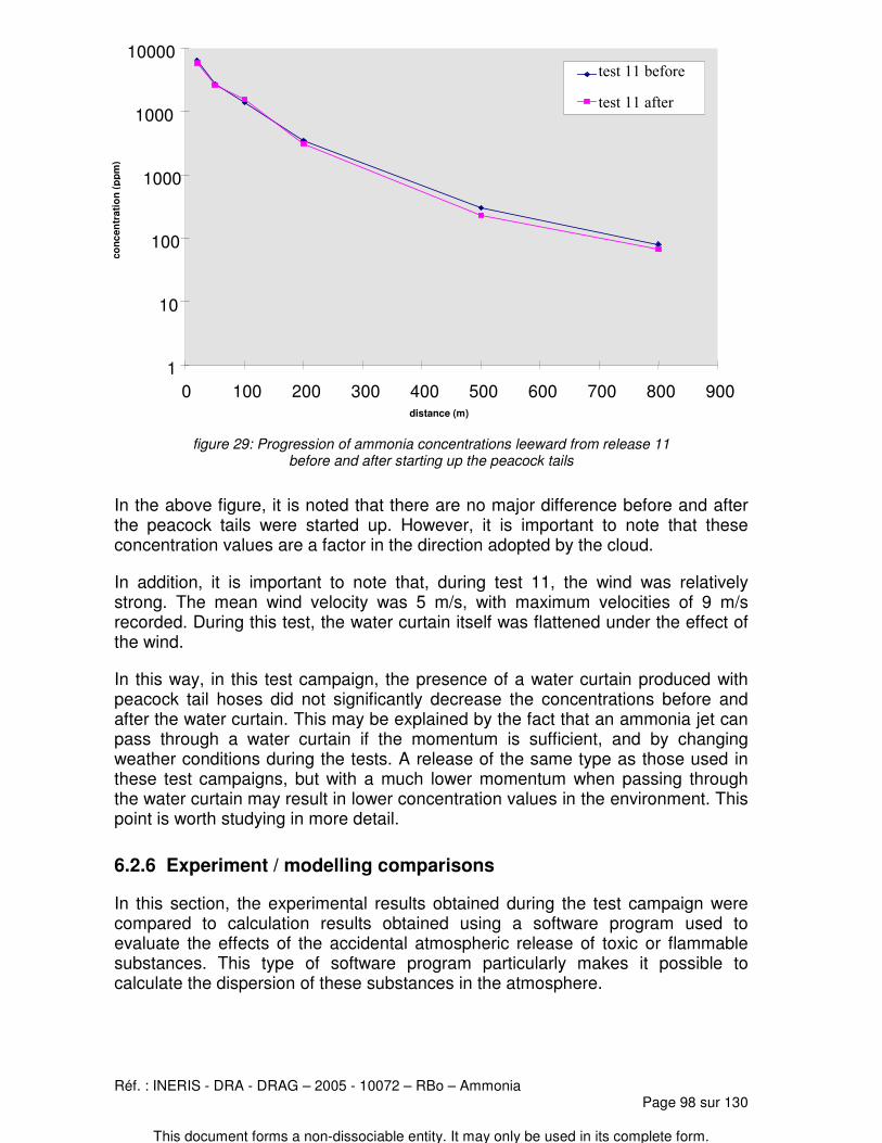
Réf. : INERIS - DRA - DRAG – 2005 - 10072 – RBo – AmmoniaPage 98 sur 130
This document forms a non-dissociable entity. It may only be used in its complete form.
figure 29: Progression of ammonia concentrations leeward from release 11before and after starting up the peacock tails
In the above figure, it is noted that there are no major difference before and afterthe peacock tails were started up. However, it is important to note that theseconcentration values are a factor in the direction adopted by the cloud.
In addition, it is important to note that, during test 11, the wind was relativelystrong. The mean wind velocity was 5 m/s, with maximum velocities of 9 m/srecorded. During this test, the water curtain itself was flattened under the effect ofthe wind.
In this way, in this test campaign, the presence of a water curtain produced withpeacock tail hoses did not significantly decrease the concentrations before andafter the water curtain. This may be explained by the fact that an ammonia jet canpass through a water curtain if the momentum is sufficient, and by changingweather conditions during the tests. A release of the same type as those used inthese test campaigns, but with a much lower momentum when passing throughthe water curtain may result in lower concentration values in the environment. Thispoint is worth studying in more detail.
6.2.6 Experiment / modelling comparisons
In this section, the experimental results obtained during the test campaign werecompared to calculation results obtained using a software program used toevaluate the effects of the accidental atmospheric release of toxic or flammablesubstances. This type of software program particularly makes it possible tocalculate the dispersion of these substances in the atmosphere.
1
10
100
1000
1000
10000
0 100 200 300 400 500 600 700 800 900distance (m)
conc
entr
atio
n (p
pm)
������1�2� �
�������2��

Réf. : INERIS - DRA - DRAG – 2005 - 10072 – RBo – AmmoniaPage 99 sur 130
This document forms a non-dissociable entity. It may only be used in its complete form.
Of the software available, PHAST software version 4.2 was used. This model is ofthe integral type, i.e. it can be used to solve conservation equations based onsimplifying hypotheses. With this respect, the limitations inherent to this softwareare particularly as follows:
� the site must be flat, of uniform roughness and not obstructed withobstacles ;
� the wind velocity must be at least equal to 1 m/s to obtain plausible results ;
� the weather conditions must be invariable throughout the emission anddispersions time ;
� the release source term must be constant over time.
To make the dispersion calculations for a substance in the atmosphere, it isnecessary to define the source term of the release and the weather conditions inwhich it is dispersed in the model beforehand.
In chapter 5, we saw that the determination of the source term of a release with amodel could give different results to that measured in reality. In order to do awaywith the source term problem (the subject of this section being the study ofdispersion in the atmosphere), the comparisons were made as follows. Firstly, theparameters measured in the tank for a given release were entered in the softwareand, secondly, the other parameters such as the regular and irregular pressuredrops were adjusted so as to calculate a mass flow rate identical to the flow ratemeasured experimentally.
Then, the meteorological data measured during the test were entered on the basisof the experimental data (ambient temperature, relative humidity, etc.). The meanwind velocity during the test was selected for the calculations. With respect to theatmospheric stability, we selected those which were calculated using the twomethods described in chapter 5. If the two methods gave different stability classes,both classes were used for the calculations.
With these conditions entered in the software, firstly, we calculated the dispersionof ammonia in the atmosphere for open-field releases, i.e. tests 1, 2, 2b, 4, 10, 11and 12.

Réf. : INERIS - DRA - DRAG – 2005 - 10072 – RBo – AmmoniaPage 100 sur 130
This document forms a non-dissociable entity. It may only be used in its complete form.
The 4 graphs given in the figure below show a comparison between theexperimental results (blue curve) and the results of dispersion calculations in theatmosphere.
figure 30: Comparisons between calculation resultsand experimental results for tests 4, 10, 2 and 2b
In these graphs, it can be seen that the software calculates ammoniaconcentration values of the same order of magnitude as the values measuredexperimentally. Only test 2b, among the open-field releases, resulted in thecalculation of two concentration values 100 m and 200 m from the release pointwhich were significantly lower than the experimental values.
However, as a general rule, the modelling of the dispersion in the atmosphere of aliquefied gas release such as ammonia gives comparable orders of magnitude tothat observed for large-scale releases, provided that:
� the source term is determined correctly in the software ;
� the weather conditions are defined correctly, given that they may varyrapidly over time (both the wind velocity and the atmospheric stability ;
� the release is carried out horizontally, in the direction of the wind, on a flatsite and with no obstacles.
Secondly, we made calculations with impacting releases. The figure below showsthe progression of the experimental concentrations (blue curve) and theconcentrations calculated with the model for releases against a wall (tests 5 and 6)and on the ground (tests 7 and 8b).
1
10
100
1000
10000
100000
0 100 200 300 400 500 600 700 800 900
distance (m)
conc
entr
atio
n (p
pm)
4 (C/D3) exp
4 (C3)
4 (D3)
1
10
100
1000
10000
100000
0 100 200 300 400 500 600 700 800 900
distance (m)
conc
entr
atio
n (p
pm)
10 (A/B3) exp
10 (A3)
10 (B3)
1
10
100
1000
10000
100000
0 100 200 300 400 500 600 700 800 900
distance (m)
conc
entr
atio
n (p
pm)
2 (C/D3) exp
2 (C3)
2 (D3)
1
10
100
1000
10000
100000
0 100 200 300 400 500 600 700 800 900
distance (m)
conc
entr
atio
n (p
pm)
2b (A/B4) exp
2b (A4)
2b (B4)

Réf. : INERIS - DRA - DRAG – 2005 - 10072 – RBo – AmmoniaPage 101 sur 130
This document forms a non-dissociable entity. It may only be used in its complete form.
figure 31: Comparisons between calculation resultsand experimental results for tests 5, 6, 7 and 8b
In this figure, it can be seen that, 20 m from the release point, the modelsystematically calculates a concentration approximately two times greater thanthat measured experimentally. Then, the progression of the concentrationsdepends on the atmospheric conditions. For test 6, in which these conditions wereprobably (D; 5 m/s) type, both curves (experimental and calculated) always showthe same difference during the progression of the cloud leeward from the release.The mixing of the cloud following the impact of the release, on one hand, and theretention of ammonia at the release point, on the other, may explain thisdifference.
At the present time, integral type models do not account for releases impactingsolid surfaces. Differences of the order of 50% may be observed between large-scale test results and calculations made with this type of model. Even greaterdifferences may be observed if the configuration of the impact is complex or if aretention dike is suitably positioned with respect to the release.
1
10
100
1000
10000
100000
0 100 200 300 400 500 600 700 800 900
distance (m)
conc
entr
atio
n (p
pm)
5 (A/B3,5) exp
5 (A3,5)
5 (B3,5)
1
10
100
1000
10000
100000
0 100 200 300 400 500 600 700 800 900
distance (m)
conc
entr
atio
n (p
pm)
6 (D5) exp
6 (D5)
1
10
100
1000
10000
100000
0 100 200 300 400 500 600 700 800 900
distance (m)
conc
entr
atio
n (p
pm)
7 (C/D6) exp
7 (C6)
7 (D6)
1
10
100
1000
10000
100000
0 100 200 300 400 500 600 700 800 900
distance (m)co
ncen
trat
ion
(ppm
)
8b (B/C5) exp
8b (B5)
8b (C5)


Réf. : INERIS - DRA - DRAG – 2005 - 10072 – RBo – AmmoniaPage 103 sur 130
This document forms a non-dissociable entity. It may only be used in its complete form.
7. CONCLUSION AND PROSPECTS
Within the scope of this research programme, INERIS essentially conducted a testcampaign in order to improve knowledge on the atmospheric dispersion ofammonia, particularly in open or obstructed environments.
Of all the results obtained from this test campaign, the following points are worthnoting:
� 15 tests with different configurations were conducted over the periodbetween December 1996 and April 1997 ;
� the quantity of ammonia released from the liquid phase was, depending onthe tests, between 1400 kg and 3500 kg per test over a time of between 7and 14 minutes, i.e. flow rates between 2 and 4.5 kg/s ;
� in the case of the thermodynamic progression of ammonia in the tanks,temperature and pressure measurements were made during the releases.These measurements and the interpretations are given in chapter 5 ;
� in the case of the thermodynamic progression of ammonia in the pipes, themeasurements made at the same point demonstrated that the value of thepressure is similar to the saturating vapour pressure corresponding to thetemperature measured at this point ;
� approximately 200 sensors, to measure the ammonia concentration and thetemperature, were set up for each test ;
� the ammonia cloud formed behaves like a heavy gas, and no rise in thecloud is observed ;
� the temperature in the ammonia jet can typically fall to -70°C ;
� solid obstacles (wall or ground) placed in a two-phase ammonia jet at adistance of a few metres from the release point have a major influence onthe concentration values measured after the obstacle. In this test campaign,approximately two times lower concentrations were measured after theobstacle with respect to an open-field release ;
� If the release is pointed towards the retention dike, the dike can retrieve alarge quantity of ammonia in liquid form. For two tests, quantities greaterthan 50% of the total mass released were collected in liquid form at atemperature of approximately -60°C ;
� The liquid ammonia sheet formed in this way is not evaporated rapidly ;
� water curtains produced with peacock tail hoses and located on the plumepath had little effect on ammonia dispersion under the test conditions ;

Réf. : INERIS - DRA - DRAG – 2005 - 10072 – RBo – AmmoniaPage 104 sur 130
This document forms a non-dissociable entity. It may only be used in its complete form.
� in addition, the results obtained demonstrate that the integral typedispersion models currently available can give correct orders of magnitudeof concentrations leeward from a free release. In the case of an impactingrelease, the results obtained are only correct if the models receiveinformation beforehand on the quantity released into the atmosphere (invapour or aerosol form) after the impact.
The results obtained during these tests led us to develop a new programmeintended to study the "near-field dispersion of a liquefied gas in the presence ofobstacles". The purpose of this programme, initiated in 1999 at INERIS, isparticularly to create a mathematical model used to account for the interaction of aliquefied gas release against an obstacle. In the long-term, this model could beincorporated in integral type software.

Réf. : INERIS - DRA - DRAG – 2005 - 10072 – RBo – AmmoniaPage 105 sur 130
This document forms a non-dissociable entity. It may only be used in its complete form.
8. BIBLIOGRAPHY
Air Liquide, Encyclopédie des gaz, 1980.
AUBURTIN, PICHARD, SCHORSCH, Toxicité aiguë de l'ammoniac, rapportINERIS, May 1999.
BARA, DUSSERRE, The use of water curtains to protect firemen in case of heavygas dispersion, Journal of Loss prevention in the process industries, vol. 10, No. 3,pp 179-180, 1997
B.I.T. (Bureau International du Travail), La Maîtrise des Risques d'AccidentMajeur, guide pratique, Geneva, 1993.
BLANKEN, Behaviour of ammonia in the event of a spillage, Ammonia safetyplant, 22, 1980, quoted by Wheatley (April 1987).
BIGOT, Modélisation de la perte de confinement d'un gaz liquefiés, Ecole desMines de Saint-Etienne, Euroforum, June 1996.
BOUET, Essais de dispersion atmosphérique, INERIS, Rapport annuel, 1996.
BOUET, Essais de dispersion atmosphérique, INERIS, Rapport annuel, 1997.
BUCKLEY and HUSA, Combustion Properties of Ammonia, ChemicalEngineering Progress vol. 58, No. 2, p. 81-84, 1962.
BRETHERIK, Handbook of Reactive Chemical Hazards, ed Butterworths, 4th ed,1990.
CCPS, Guidelines for consequence analysis of chemical releases. AIChE, CCPS,0003028, p-741, 1999.
ABIVEN, CHAINEAUX, Caractéristiques d'inflammabilité et d'explosibilité del'ammoniac, Rapport INERIS, EXP-FAB/DG F42 e/349 91.78.1120, 1991.
CHAINEAUX, EMERGE project (Extended Modelling and Experimental into GasExplosion), 2nd progress report, INERIS, January 1995.
DELHAYE, Les écoulements diphasiques gaz, liquide en conduite, Entropie, n°99, pp 3-25, 1981, quoted by May (1996).
EMFA (European Fertilizer Manufacturer's Association, Zurich), IFA (InternationalFertilizer Industry Association Limited, Paris), Hazardous properties of ammonia,1990, quoted by SNIE (1991).
FAUSKE, Two phase and one component critical flow. Symp. on two phase flow,Ed. P.M.C. Lacey, U. of Exeter, vol 1, pp101-114, 1965.
Réf. : INERIS - DRA - DRAG – 2005 - 10072 – RBo – AmmoniaPage 106 sur 130
This document forms a non-dissociable entity. It may only be used in its complete form.
FAUSKE, Flashing flows or some practical guidelines for emergency releases,Plant operation progress, vol. 4, No. 3, p. 132, 1985.
FLETCHER, Flashing flow through orifices and pipes, CEP, March 1984.
FULLERINGER, Evaluation de la sûreté des installations utilisant de l'ammoniac,rapport IPSN, DES n° 252, 1995.
GIFFORD, Diffusion in the Diabatic Surface Layer, J. Geophy. Res., vol. 67, no. 8,pp. 3207-3212, 1962.
GIFFORD, An outline of theories of diffusion in the lower layers of the atmosphere.Meteorology and Atomic Energy, US Atomic Commission, D.H. Slade Edition,1968.
GOLDER, Relations among stability parameters in the surface layer, Boundarylayer meteorology, 3, pp 47-58, 1972.
GOLDWIRE et al., Desert Tortoise series data report – 1983 pressurized ammoniaspills, UCID 20652, December 1985.
GOLDWIRE, Large-Scale Ammonia Spill Tests. A series of ammonia spill testsfound that improved simple models are needed for predicting the consequences ofaccidental releases. Chemical Engineering Progress, pp 35-41, April 1986.
As above: article containing comments, published in ammonia plant safety, Vol.26, pp 203-211, 1986.
HANNA, DAVID, CHANG, Evaluation of fourteen hazardous gas models withammonia and hydrogen fluoride field data, Journal of hazardous materials, Vol. 26,pp 127-158, 1991.
HANNA, CHANG, STRIMAITIS, Hazardous gas model evaluation with fieldobservations, Atmospheric Environment, Vol. 27A, No. 15, pp 2265-2285, 1993.
HODIN, Modélisation du debit à la brèche et du jet géneré par une fuited'ammoniac en phase liquide ; état des connaissances et modélisation des rejetsdiphasiques, EdF, Centre Lyonnais d'Ingénierie, Note d'étude, 1995.
IANELLO, ROTHE, WALLIS, Aerosol Research Program: improved source termdefinition for modeling the ambient impact of accidental release of hazardousliquids, Paper presented at the 6th International Symposium on Loss Preventionand Safety Promotion on the Process Industries, Oslo, Norway, 1989.
INRS, Réaction chimiques Dangereuses, ammoniac, note 1024-84-76, 1976.
INRS, Les Mélanges Explosifs, édition de 1989, A. CLEUET.
INRS, Fiche Toxicologique n° 16, gaz ammoniac et solutions aqueuses, éditionrévisée, 1992.

Réf. : INERIS - DRA - DRAG – 2005 - 10072 – RBo – AmmoniaPage 107 sur 130
This document forms a non-dissociable entity. It may only be used in its complete form.
KIRK-OTHMER, Encyclopedia of Chemical Technology, 3rd ed., vol. 2, p. 470-516,1978.
KOOPMAN, McRAE, GOLDWIRE, ERMAK, KANSA, Results of Recent Large-Scale NH3 and N2O4 Dispersion Experiments, S. Hartwig (ed.), Heavy Gas andRisk Assessment – III, p 137-156, 1986.
KRAMER, Minimum ignition energy of ammonia-air mixture, Gas discharges,Their Appl. Proc. Int. Conf. 8th, 1985.
LANGARD, ANSTETT, MAVROTHALASSITIS, La prise en compte desphénomènes biphasiques dans l'analyse des risques, Rapport INERIS, October1995.
LANTZY, Vapor cloud source modeling workshop, Chairman’s report,Plant/Operations Progress, Vol. 11, No. 1, pp 41-45, 1992.
LEUNG, Two-phase flow discharge in nozzles and pipes, a unified approach, J.Loss Prevention Ind., vol.3, pp 27-32, January 1990.
MAY, Ecoulements diphasiques lors de la vidange de gaz liquéfiés initialementsous saturés, validation par l’eau et le CFC11, Thèse de l’école des Mines deSaint-Etienne et de Paris, 1996.
MEDARD, Les explosifs occasionnels, vol. 1, p. 210-211-213-261, 1979.
NFPA (National Fire Protection Association), No. 325 M, 1990.
NFPA (National Fire Protection Association), Fire Protection Guide to HazardousMaterials, 11th edition, 1994.
NIOSH (National Institute for Occupational Safety and Health), pocket guide tochemical hazards, 1987.
NIELSEN and OTT, Fladis Field Experiments, Final Report, RISØ-R-898(EN),July 1996.
NYRÉN, WINTER, Two-phase discharge of liquefied gases through pipes, fieldexperiments with ammonia and theoretical model, 4th international symposium onloss prevention and safety promotion in the process industries, No. 33, vol. 1, p E1-E 11, 1983
NYRÉN et al., Discharge trials with liquefied ammonia at Simpra, Landskrona,Sweden, Swedish National Defence Research Institute, FOA report E40009, 1983,quoted by Wheatley (April 1987).
PASQUILL, The Estimation of the Dispersion of Windborne Material, Meteorol.Mag., vol. 90, pp. 33-49, 1961.
PASQUILL, Atmospheric diffusion, 2nd edition, Ellis Howood, London, 1974.

Réf. : INERIS - DRA - DRAG – 2005 - 10072 – RBo – AmmoniaPage 108 sur 130
This document forms a non-dissociable entity. It may only be used in its complete form.
REED, Containment of leaks from vessels containing liquefied gases withparticular reference to ammonia, 1st international symposium on loss preventionand safety promotion in the process industries, The Hague, pp. 191-195, Elsevier,1974, quoted by Wheatley (April 1987).
RESPLANDY, Etude des prescriptions à préconiser pour la sécurité du voisinagedes dépôts d’ammoniac liquide. Compte-rendu des expériences effectuées le 28juin 1967. Comité Consultatif des Etablissements Classés. September 1967.
RESPLANDY, Etude des mesures à préconiser pour la sécurité du voisinage desstockages d’ammoniac liquéfié. Comité Consultatif des Etablissements Classés.December 1968.
RESPLANDY, Etude expérimentale des propriétés de l’ammoniac conditionnantles mesures à prendre pour la sécurité du voisinage des stockages industriels.Chimie et Industrie - Génie chimique, Vol. 102, n°6, October 1969.
RIOU, Comment estimer la dispersion des gaz lourds?, EdF bulletin de la directiondes études et recherches, série A, Nucléaire, hydraulique, thermique, 1989.
SAX’S Dangerous properties of industrial materials, 9th edition, 1996.
S.E.I. (Service de l’Environnement Industriel, du Ministère de l’Aménagement duTerritoire et de l'PEnvironnement), fiches techniques, courbes de toxicité parinhalation, 1998.
S.N.I.E. (Syndicat National de l’Industrie des engrais), Aide-mémoire sur lesrisques présentés par l’ammoniac, 1991.
TISSOT, PICHARD, Seuils de toxicité aiguë, Ammoniac, 2003. (seewww.ineris.fr).
TURNER, Workbook of Atmospheric Dispersion Estimates, US, Department ofHealth Education and Welfare, NTIS, Cincinnati, Ohio, 1970.
U.I.C. (Union des Industries Chimiques), Emission à la brèche d’une capacité,débit en phase gaz, débit en phase liquide, formation et vaporisation des flaques,Cahiers de sécurité n°11, September 1987.
U.I.C. (Union des Industries Chimiques), Dispersion atmosphérique, Groupe detravail Prévention des risques majeurs, Cahier de Sécurité n°6, June 1995.
ULMANN, Encyclopedia of lndustrial Chemistry, 5th edition, vol. A2 p. 143-242,1985.
VAN DEN HAKKER, SNOEY, SPOELSTRA, Discharges of pressurized liquefiedgases through apertures and pipes, 4th international symposium on loss preventionand safety promotion in the process industries, No. 33, vol. 1, pp E23-E35, 1983.

Réf. : INERIS - DRA - DRAG – 2005 - 10072 – RBo – AmmoniaPage 109 sur 130
This document forms a non-dissociable entity. It may only be used in its complete form.
WEISS, Hazardous Chemicals Data Book, NDC (Noyes Data Corporation),2nd edition, 1985.
WHEATLEY, A theoretical study of NH concentrations in moist air arising fromaccidental releases of liquefied, using the computer code TRAUMA, Health andSafety Executive; SRD/HSE/R 393, February 1987.
WHEATLEY, Discharge of liquid ammonia to moist atmospheres - Survey ofexperimental data and model for estimating initial conditions for dispersioncalculations, Health and Safety Executive; SRD/HSE/R 410, April 1987.
WHO (World Health Organisation), IPCS, Environmental Health Criteria 54,Ammonia, 1986.
WOODWARD, Expansion zone modeling of two phase and gas discharges, J. ofHazardous materials, 33, pp 307-3 18, 1993.
WOODWARD, PAPADOURAKIS, Modeling of droplet entrainment andevaporation in dispersing jet, in CCPS (1971), pp 147-167.
YAN, Modélisation de l’autoévaporation en écoulements subcritiques et critiques,thesis, U. Catholique de Louvain, Belgium, 1991, quoted by May (1996).
ZAKAZNOV, KURSHEVA, FEDINA, Determination of Normal Flame Velocity andCritical Diameter of Flame Extinction in Ammonia-Air Mixture, Combustion,Explosion and Shock Waves, No. 6, vol. 14, p. 710-713, 1978.

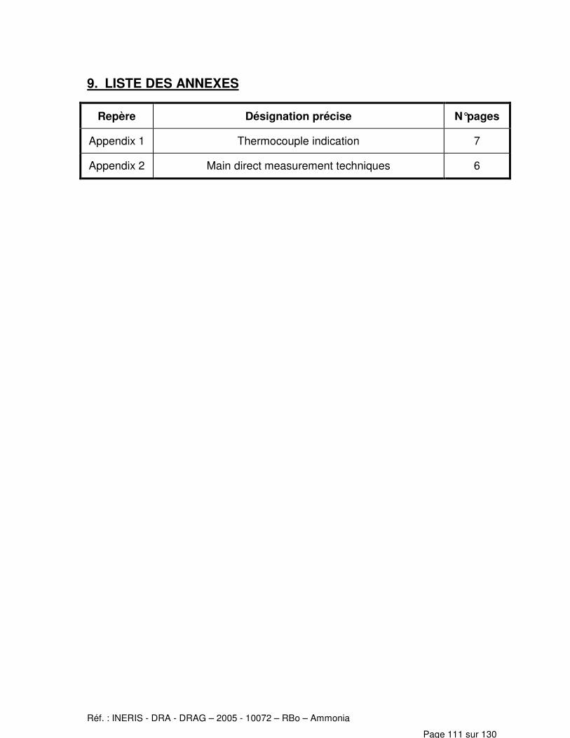
Réf. : INERIS - DRA - DRAG – 2005 - 10072 – RBo – Ammonia
Page 111 sur 130
9. LISTE DES ANNEXES
Repère Désignation précise N°pages
Appendix 1 Thermocouple indication 7
Appendix 2 Main direct measurement techniques 6


Réf. : INERIS - DRA - DRAG – 2005 - 10072 – RBo – Ammonia
Page 113 sur 130
APPENDIX 1
THERMOCOUPLE INDICATION


Réf. : INERIS - DRA - DRAG – 2005 - 10072 – RBo – Ammonia
Page 115 sur 130
The thermocouples referred to in this appendix are those which were installed:
� in the ammonia tank,
� on the release system,
� on the release slab,
� and, if applicable, on the wall or retention dike.
A description of the location of the thermocouples is given in the table below.
For all the tests, the following thermocouples were installed:
Thermocouplelocation Caption
in tank 1450 mmfrom base Tank 1450 mm
in tank 1100 mmfrom base Tank 1100 mm
in tank 750 mm frombase Tank 750 mm
in tank 400 mm frombase Tank 400 mm
in tank 50 mm frombase Tank 50 mm
at end of releasesystem OUTLET – th6
between two releasesystem valves th 7
at inlet of releasesystem th 8

Réf. : INERIS - DRA - DRAG – 2005 - 10072 – RBo – Ammonia
Page 116 sur 130
Test 4:
For this test, four additional thermocouples were installed on the ground. Two inthe direction of the release 3 and 5 metres from the orifice and two on either sideat 3 metres.
Thermocouplepositions Caption
on ground, in direction ofrelease (27), 3 metres
from orificeground dir 27 at 3m
on ground, in direction ofrelease (27), 5 metres
from orificeground dir 27 at 5m
on ground, in direction ofrelease (23), 3 metres
from orificeground dir 23 at 3m
on ground, in direction ofrelease (31), 3 metres
from orificeground dir 31 at 3m
Tests 5 and 6:
With respect to these tests, a 3 metres wide, 3 metres high and 1 metre thick wallwas constructed at a distance from the orifice of 3 metres and 1 metre,respectively. For both configurations, 19 thermocouples were installed, 4 on thewall and 15 on the ground.
On the wall, the 4 thermocouples referenced 11 to 14 were installed as describedin figure 32 below.
�� ����
��
figure 32
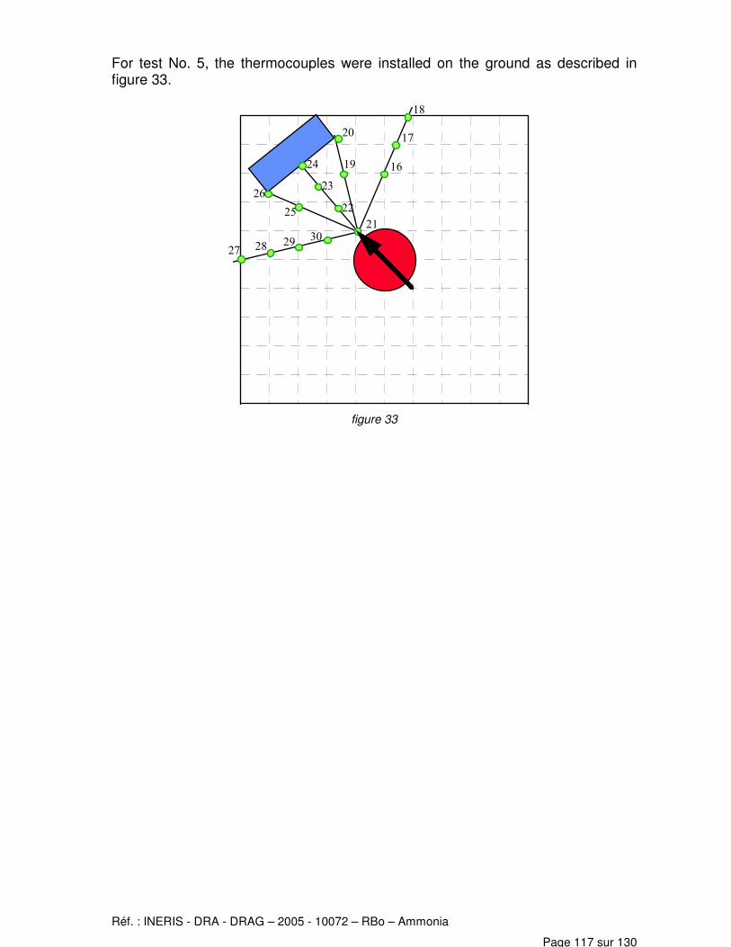
Réf. : INERIS - DRA - DRAG – 2005 - 10072 – RBo – Ammonia
Page 117 sur 130
For test No. 5, the thermocouples were installed on the ground as described infigure 33.
����
�-
���- ��
��
��
��
��
��
��
��
��
��
figure 33

Réf. : INERIS - DRA - DRAG – 2005 - 10072 – RBo – Ammonia
Page 118 sur 130
The caption used for each of these thermocouples is given in the table below.
Caption
th11 – wall 1 mcentre
th21 – groundcentre
th12 – wall 1 mright
th22 – groundcentre
th13 – wall 1 m left th23 – groundcentre
th 14 – wall 2 mcentre th24 – ground centre
th16 – ground 60°right
th25 – ground 30°left
th17 – ground 60°right
th26 – ground 30°left
th18 – ground 60°right
th27 – ground 60°left
th19 – ground 30°right
th28 – ground 60°left
th20 – ground 30°right
th29 – ground 60°left
th30 – ground 60°left

Réf. : INERIS - DRA - DRAG – 2005 - 10072 – RBo – Ammonia
Page 119 sur 130
For test 6, the wall was located one metre from the release system orifice.Therefore, the thermocouples were installed on the ground as shown in figure 34below.
��
��
�-
��
�-
��
��
��
��
����
����
��
��
figure 34
Tests 7 and 8: These tests were instrumented as follows (see figure 35):
�� ���-
��
�-
��
��
��
��
��
��
��
��
��
��
��
��
��
��
figure 35

Réf. : INERIS - DRA - DRAG – 2005 - 10072 – RBo – Ammonia
Page 120 sur 130
Test 9:
For this test, the end of the release system impacted into a 2m x 2m x 1mretention dike. The thermocouples were installed along the direction 20, asdescribed in the figure below.
�� ����
��
���-������ ���� �� ��
�����-
��
��
��
�$����$��
���� ���� ����
height /ground (mm) thermocouples
0 th11 th27 th28 th29
30 th12
60 th13
100 th14
150 th15
200 th16
300 th17
400 th18
500 th19 th26
600 th20
800 th21
1000 th22 th23 th24 th25

Réf. : INERIS - DRA - DRAG – 2005 - 10072 – RBo – Ammonia
Page 121 sur 130
Tests 10, 11 and 12:
For these three tests, 6 thermocouples were installed on the ground along the axisof the release system. From the vertical line from the release point, there was oneevery metre. We indicated them as follows:
��
����
�� �� ��
��
��
� �#����
� �#����
� �#����
� �#����
� �#����
� �#����
figure 36
Tests 2b and 8b:
For these two tests, in addition to the 6 thermocouples described above, weinstalled 12 on two masts, and 1 to 50 cm above the release orifice. The latter isindicated in the caption: "point 0 – h=1.5m". The other thermocouples areindicated as follows on masts 1 and 2, located 2 and 4 metres from point 0 in thedirection 7, respectively.
������! �0��
������! �0��
������! ��
������! �0��
������! ��
������! ��
������! �0��
������! �0��
������! ��
������! �0��
������! ��
������! ��
figure 37


Réf. : INERIS - DRA - DRAG – 2005 - 10072 – RBo – Ammonia
Page 123 sur 130
APPENDIX 2
MAIN DIRECT MEASUREMENT TECHNIQUES


Réf. : INERIS - DRA - DRAG – 2005 - 10072 – RBo – Ammonia
Page 125 sur 130
The purpose of appendix 2 is to give a brief presentation of the main ammoniaconcentration measurement techniques. This chapter is particularly based on thework by A. Accorsi's team [1,3] and the documentation supplied by themanufacturers, particularly [2,4].
1 ELECTROCHEMICAL CELL DEVICES
This section is essentially based on document [1].
Device to measure gas concentrations in the air using electrochemical cellsemerged approximately twenty years ago.
Measurement principle
Each electrochemical cell is relatively specific for the detection of a single gas. Thegas to be measured passes through a semi-permeable membrane, i.e. permeablefor gases but impermeable for liquids. The gas comes into contact with a sensitiveelectrode coated in a catalyst in the presence of which, it is oxidised, while acounter-electrode reduces the oxygen in the air. These oxidation-reductionphenomena are accompanied by an ion flow through the electrolyte and anelectron flow to the outside. (See Figure 2.1)
The reaction to the sensitive electrode is (according to MARTEC documentation):
2 NH3 --------> N2 + 6 e- + 6 H+
The reaction to the counter-electrode is (according to the CECA report):
2 e- + 0.5 O2 + 2 H+ -------> H2O
Overall:
2 NH3 + 3/2 O2 -------> N2 + 3 H2O

Réf. : INERIS - DRA - DRAG – 2005 - 10072 – RBo – Ammonia
Page 126 sur 130
To avoid capacitive limit layer phenomena at the electrode/electrolyte interface, areference electrode maintains the potential of the sensitive electrode at a fixedvalue, which makes it possible to keep a signal stable over time.
Figure 2.1: Functional description of an electrochemical cell(diagram p 44 fig. 5 in CECA report [1])
Limitations
Selectivity is obtained, firstly, with the value of the reference potential and,secondly, with the oxidation catalyst. In practice, absolute selectivity does notexist. For example, the table below, given by Dräger, shows some compoundsinducing interference on PAC II NH3:
Gas Symbol Test gasconcentration (V/V)
Deviation in ppmNH3 from
measurement value
Chlorine Cl2 10 ppm < 1
Cyanhydric acid HCN 25 ppm < 3
Carbon dioxide CO2 1% -5 < and < 0 (defaultsignal)
Carbon monoxide CO 115 ppm < 3
Methane CH4 30% < 3
Methanol CH3OH 170 ppm < 35
Sulphur anhydride SO2 20 ppm <1
Hydrogen sulphide H2S 20 ppm < 75
Nitrogen dioxide NO2 20 ppm < 3
Hydrogen H2 1.53% < 115
Table 2.1: Compounds inducing interference on PAC II NH3, based on Dräger's technicaldocumentation for PAC II NH3
In this way, it is difficult to know exactly what is being measured and, in particular,how accurate the measurement is, in the case of an environment in which severalgases are present (for example, in industrial atmospheres).

Réf. : INERIS - DRA - DRAG – 2005 - 10072 – RBo – Ammonia
Page 127 sur 130
The measurement range of the majority of electrochemical type devices, formeasuring ammonia concentrations, is from a few ppm to 300, 500 or 1000 ppm.Cells capable of measuring around one thousand ppm are very rare. The limit ofdetection is of the order of 20 to 30 ppm. The response time is in excess of 20 sand may be up to one minute, and depends on the type of membrane used toprotect the sensitive electrode. The service life of this type of device isapproximately one to two years. The average price of an electrochemical cellalone is approximately 1000 FF and varies from 500 to 7000 FF.
2 CATALYTIC OXIDATION DEVICES (PELLISTOR)
This section proposes a summary of the EEV [2] and INRS [3] technicaldocuments.
Principle
The principle consists of inducing the catalytic oxidation of the flammable gas, inthis case, ammonia, and measuring the heat produced.
In fact, the catalytic detector is equipped with two components: an active catalyticdetector and a non-active compensator component. Each component consists of aplatinum filament in a bead of heat-resistant material. For the detector component,a catalytic mixture is applied to this bead, while for the compensator component,the bead is treated such that catalytic oxidation cannot occur.
The two components are connects in a Wheatstone bridge as shown in figure 2.2taken from the document [3].
Figure 2.2: Principle diagram of catalytic oxidation measurement device(INRS diagram)

Réf. : INERIS - DRA - DRAG – 2005 - 10072 – RBo – Ammonia
Page 128 sur 130
The direct current flowing through the beads brings the detector to a suitabletemperature for the gas to be detected. The detector filament works like athermometer: when the combustible gas is oxidised on the detector bead, theresulting temperature rise increases filament resistance. This unbalances thebridge, giving a signal that can be read, either as a gas percentage, or as apercentage of the Lower Explosibility Limit (LEL), or that triggers an audio or visualalarm.
The rate at which the gas will burn on the detector component depends on the gasdiffusion rate in the detector. The diffusion rate is controlled by enclosing thecomponents in a unit of precise dimensions.
In addition, EEV explains that there are two assembly arrangements. In the first,the gases circulate at a given flow rate of 0.5 litre/minute. The secondarrangement is designed for simple gas diffusion in a unit. In both cases, a frit isincluded and a paper filter is placed in the diffusion head to prevent dust frompenetrating into the cavity. Another possibility consists of replacing the frit with adisk of tiny bronze or stainless steel beads (recommended for ammonia).
Limitations
The service life of the detector is limited. It is associated with the operatingtemperature, and also with a loss of efficiency over time, which depends onprolonged operation, exposure to excessively high concentrations. Finally, thedetector may be damaged ("poisoned") by some gases or vapours. To protect thedetector from the effects of some organic or silicone-based vapours, aninterchangeable activated charcoal or carbon filter may be used.
The bridge output signal is of the type represented in figure 2.3. It rises above theLEL (Lower Explosibility Limit), up to the stoichiometric value which isapproximately 10% in air for methane (example represented below) and 21% forammonia. For higher concentrations, the signal declines in a linear fashion due tothe lack of oxidant.
It can be noted that, when the combustible gas concentration exceeds thestoichiometric value, it is possible to use another type of detector based on thethermal conductivity principle to measure high concentrations and thus eliminateany doubt with respect to ambivalence. As such, the compensator components ofsome catalytic oxidation detectors may be used. However, according to theinformation supplied by EEV, the thermal conductivity of ammonia is very similar tothat of air, so much so that it may be impossible, or very difficult, to make anaccurate, detailed measurement.

Réf. : INERIS - DRA - DRAG – 2005 - 10072 – RBo – Ammonia
Page 129 sur 130
Figure 2.3: Pellistor type sensor output signal for exposure to methane (diagram from EEV brochure)
Concentrations greater than the stoichiometric value may be measured by dilutingwith air according to a known dilution ratio, e.g. 10. In this way, 100% v/v ammoniawould be lowered to 10% and the detection sensitivity would be of the order of1% v/v.
3 SEMICONDUCTORS
The documents [3,4] were used to prepare this section.
Principle
A semiconductor is a material in which the electricity conducting properties areintermediary between those of a conductor and those of an insulator. Thepresence of a gas induces a variation in the electrical resistance of thesemiconductor components of the detector by means of physical adsorption(reversible phenomenon) and catalytic combustion phenomena on thesemiconductor surface; the adsorbed gas is oxidised in the presence of surfaceoxygen and the combustion product is desorbed. Modifying the oxygen content onthe surface induces a modification in the electron-hole equilibrium (the hole beingthe adsorption site) in the semiconductor. This variation is directly linked with thegas concentration and modifies the electrical equilibrium of the circuit in which thedetector is placed.
In the case of the Figaro detector, the semiconductor material used is tin dioxide(SnO2-X) which is heated to a high temperature (e.g. 400°C).
Limitations
Semiconductor detectors are very temperature-sensitive: the conductibilityincreases with the temperature. In addition, semiconductor operation is disturbedby interfering parameters such as humidity, dust, grease of other preferentiallyadsorbed gases.

Réf. : INERIS - DRA - DRAG – 2005 - 10072 – RBo – Ammonia
Page 130 sur 130
Bibliographic References
[1] Accorsi. Rapport final CECA – Faisabilité de campagnes de mesuresd'atmosphères de travail par des appareils multigaz transportables. 1992
[2] EEV. Combustible Gas Detectors – Product Data
[3] A. Accorsi, J. C. Laforest, P. Huré. Détection de mélanges air-ammoniac.INRS. Cahiers de notes documentaires n°127, p 217-222, 2e trimestre 1987.
[4] FIGARO – Products Catalog.
