Amphibian stress, survival, and habitat quality in restored agricultural wetlands

in central Iowa

by

Rebecca Ann Reeves

A thesis submitted to the graduate faculty

in partial fulfillment of the requirements for the degree of

MASTER OF SCIENCE

Major: Wildlife Ecology

Program of Study Committee:

Clay L. Pierce, Major Professor

Erin Muths

Robert Klaver

Jarad Niemi

Iowa State University

Ames, Iowa

2014

Copyright © Rebecca Ann Reeves, 2014. All rights reserved.

ii

TABLE OF CONTENTS

Page

ACKNOWLEDGEMENTS ..................................................................................................... iv

ABSTRACT .............................................................................................................................. v

CHAPTER 1. INTRODUCTION ............................................................................................. 1

Background ........................................................................................................................... 1

Goals and Objectives ............................................................................................................ 2

Thesis Organization .............................................................................................................. 2

Literature Cited ..................................................................................................................... 3

CHAPTER 2. AMPHIBIAN STRESS, SURVIVAL, AND HABITAT QUALITY IN

RESTORED AGRICULTURAL WETLANDS IN CENTRAL IOWA .................................. 5

Abstract ................................................................................................................................. 5

Introduction ........................................................................................................................... 6

Methods................................................................................................................................. 9

Study Wetlands .................................................................................................................. 9

Environmental Characteristics......................................................................................... 10

Amphibian Characteristics .............................................................................................. 11

Results ................................................................................................................................. 15

Environmental Characteristics ........................................................................................ 15

Amphibian Characteristics .............................................................................................. 16

Discussion ........................................................................................................................... 19

Environmental Characteristics ........................................................................................ 19

Amphibian Characteristics .............................................................................................. 22

Acknowledgements ............................................................................................................. 24

Literature Cited ................................................................................................................... 25

Tables .................................................................................................................................. 31

Figures................................................................................................................................. 36

CHAPTER 3. AMPHIBIANS, PESTICIDES, AND THE AMPHIBIAN CHYTRID

FUNGUS IN RESTORED AGRICULTURAL WETLANDS............................................... 41

Introduction ......................................................................................................................... 41

Methods............................................................................................................................... 43

Study Wetlands ................................................................................................................ 43

Environmental Sampling ................................................................................................. 43

Amphibian Sampling ....................................................................................................... 44

Statistical Analysis .......................................................................................................... 45

Results ................................................................................................................................. 46

Discussion ........................................................................................................................... 48

iii

Acknowledgements ............................................................................................................. 50

Literature Cited ................................................................................................................... 50

Tables .................................................................................................................................. 54

Figures................................................................................................................................. 60

CHAPTER 4. CONCLUSIONS ............................................................................................. 62

Summary ............................................................................................................................. 62

Literature Cited ................................................................................................................... 64

APPENDIX A. SUPPLEMENTARY TABLES..................................................................... 66

APPENDIX B. EXPANDED METHODS ............................................................................. 68

Environmental Sampling .................................................................................................... 68

Amphibian Sampling .......................................................................................................... 69

Literature Cited ................................................................................................................... 70

APPENDIX C. CORRELATION MATRICES ...................................................................... 72

APPENDIX D. SUPPLEMENTARY FIGURES ................................................................... 73

APPENDIX E. COMPLETE MODEL SELECTION RESULTS .......................................... 75

APPENDIX F. PESTICIDE DETECTION MATRIX ........................................................... 78

APPENDIX G. DETECTION LIMITS .................................................................................. 80

APPENDIX H. PARASITE ANALYSIS RESULTS ............................................................. 83

iv

ACKNOWLEDGEMENTS

First, I would like to thank all of my friends and family for their support and

encouragement. You all have been such a blessing and I especially appreciate your help with

everything, including editing. Also, I could probably do dishes and housework from now until

eternity and it would only start to make up for Chad’s support while I was writing. Thank you! I

have been privileged to have some of the best office mates around and they have provided

invaluable advice and much needed dance parties. I will miss you guys! I would also like to

thank all of my technicians and the army of volunteers that helped me to catch frogs and collect

data- I couldn’t have done it without you!

I would like to thank my committee chair, Clay Pierce, and my committee members, Erin

Muths, Bob Klaver, and Jarad Niemi, for their guidance and support throughout the course of

this research. I would also like to thank Kelly Smalling, Mark Vandever, and Bill Battaglin for

their help and encouragement. It has been a real pleasure working with all of you and I have

learned so much!

v

ABSTRACT

Amphibians are declining throughout the United States and worldwide due to habitat

loss, emergent diseases, and chemical contaminants in the environment. Iowa is a heavily

modified landscape where 90% of the historic wetland area has been converted to row crop

agriculture. In Iowa, the Conservation Reserve Enhancement Program (CREP) strategically

restores wetlands to reduce nitrogen loads in tile drainage effluent. This project examined the

quality of amphibian habitat provided by these restored wetlands by comparing amphibian

species richness, estimated monthly survival probabilities of adult leopard frogs (Lithobates

pipiens), and developmental stress levels in leopard frogs to a suite of environmental stressors

including nutrient concentrations, water chemistry, and the presence of parasites and aquatic

predators in wetlands. We also measured the concentrations of pesticides, herbicides, and

fungicides in water and amphibian tissue samples and compared them to the prevalence of the

amphibian chytrid fungus (Batrachochytrium dendrobatidis, Bd) within the chorus frog

(Pseudacris maculata) population, as well as the abundance of zoospores in water samples and

on frog skin.

CREP and reference wetlands offer different qualities of amphibian habitat. CREP

wetlands were characterized by higher nitrogen concentrations, more alkaline pH, slightly longer

hydroperiods, and greater depths. Differences in structural characteristics may contribute to the

increased prevalence of non-native bullfrogs and fish, while high nitrogen concentrations may

increase the risk of trematode parasitism for resident amphibians. Unfortunately, these physical

characteristics are central to the primary nitrogen removal functions of CREP wetlands, so

cannot be easily avoided. Mechanical drawdowns, which are already recommended on an as-

needed basis for emergent vegetation management in CREP wetlands, could have an added

vi

benefit of reducing the impact of predators such as bullfrogs and fish on native amphibian

species. Reference wetlands had higher concentrations of Bd zoospores and a higher incidence of

developmental stress, but overall there were few differences in the composition of the amphibian

assemblage, or in the population sizes and survival probabilities of leopard frogs between

wetland types.

There were no differences in the concentrations of pesticides in water or chorus frog

tissue samples or in the abundance of zoospores of the amphibian chytrid fungus between CREP

and reference wetlands. While the concentration of zoospores in water samples was not related to

the concentration of pesticides in water samples, fungicides and non-fungicides had opposing

relationships to the prevalence of Bd in the chorus frog population. Fungicides and non-

fungicides also had opposing relationships to zoospore abundance in water and on frog skin. In

general, the abundance and prevalence of the amphibian chytrid fungus was positively correlated

with total non-fungicide concentrations and either negatively or not correlated with total

fungicide concentrations.

CREP and reference wetlands provide important habitat for amphibians in central Iowa.

Maintaining some relatively predator-free wetlands within the larger complex of wetlands with a

variety of hydroperiods appears to be important for the long term persistence of amphibians in

this landscape, especially in light of increasing variability in rainfall due to climate change.

Further study on the interactions between combinations of chemicals at ecologically relevant

concentrations and other environmental stressors, including emergent diseases, will contribute

greatly to our understanding of the effects of land use on amphibians and will aid in the

conservation of amphibians.

1

CHAPTER 1. INTRODUCTION

Background

Wetlands provide numerous services to humans and the environment, from soil erosion

control and nutrient cycling to the production of wildlife for recreational and spiritual

appreciation (Dodds et al., 2008). Amphibians are an integral part of wetland ecosystems and are

declining globally (Wake & Vredenburg, 2008). In the United States, and especially in the

Midwest, the decline of amphibians coincides with a loss of wetland area and surrounding

upland habitat as natural areas are converted to agricultural and urban uses.

In the past two hundred years, the landscape in Iowa has changed immensely (Bogue,

1963). The Des Moines Lobe landform extends from Alberta, Canada, through central Iowa and

covers approximately 700,000 km2 (Miller et al., 2009). Historically, it was characterized by a

high density of small, depressional wetlands with variable water regimes (Miller et al., 2009).

The advent of tile drainage technology allowed settlers to drain the prairie pothole wetlands of

the Des Moines Lobe, and to utilize the rich prairie soils for crop production. Since tile drainage

was first brought to Iowa in the early 1900s, 90-99% of the state’s historical wetland area has

been drained and converted to row-crop agriculture (Whitney, 1994; Miller et al., 2009). The

increased presence of row crop agriculture on the landscape has brought with it an increase in

surface water contamination from nutrients, chemicals, and sediment transported off of

agricultural fields.

In Iowa, the Conservation Reserve Enhancement Program (CREP), which is administered

by the Iowa Department of Agriculture and Land Stewardship (IDALS), strategically restores

wetlands to capture water draining from agricultural areas and improve downstream water

quality. CREP wetlands reduce nitrate concentrations and allow suspended sediment to settle out

2

(Iovanna et al., 2008). As an added ecosystem service, CREP wetlands provide habitat for

waterfowl and other wildlife (Knutson et al., 2004; O'Neal et al., 2008). This increase in wetland

habitat is also putatively beneficial to amphibians, which have been observed at many of the

restored wetlands. However, the benefits of increased habitat area may be negated if the quality

is insufficient to support sustainable amphibian populations and instead these wetlands function

as population sinks (Pulliam 1988; Dias 1996).

Goals and Objectives

This project compared the quality of amphibian habitat provided by CREP and other, reference,

wetlands with five primary objectives:

1. Record amphibian species richness at CREP and reference sites

2. Estimate lethal impacts to amphibians by estimating monthly survival probabilities of

northern leopard frogs (Lithobates pipiens) in CREP and reference wetlands

3. Monitor sub-lethal responses of leopard frogs to environmental stressors using metrics

measuring developmental stress (e.g., body condition and fluctuating asymmetry)

4. Categorize the concentrations of pesticides and pesticide degradates in boreal chorus frog

(Pseudacris maculata) tissue

5. Document environmental stressors (e.g., pesticides, predators, and disease) of amphibians

in restored and reference wetlands and compare them to amphibian responses (i.e.,

monthly survival probabilities, developmental stress levels, and disease prevalence)

Thesis Organization

After a general introduction in Chapter 1, this thesis is organized as a series of

manuscripts for submission to academic journals. Chapter 2 is formatted for submission to the

journal Wetlands and compares amphibian species richness, estimated monthly survival

3

probabilities of adult northern leopard frogs, and developmental stress levels of leopard frogs to

a suite of environmental variables including nutrient concentrations, water chemistry, and the

presence of aquatic predators and zoospores of the amphibian chytrid fungus (Batrachochytrium

dendrobatidis, Bd). Chapter 3 will be submitted to Herpetological Review and compares the

prevalence of Bd in boreal chorus frog populations as well as the concentrations of Bd zoospores

in water samples and on frog skin to the total concentrations of fungicides, non-fungicides, and

all pesticides in water and frog tissue samples. Chapter 4 outlines the general conclusions of this

study and identifies areas for future research. The appendices provide supplementary information

on the statistical modeling used to estimate the leopard frog demographic parameters, the

detection limits of pesticides in environmental and frog tissue samples, and a matrix of the

chemicals detected in water, sediment, and frog tissue samples. The appendices also hold a

number of supplementary tables and figures and a summary of the results of the

histopathological analysis of chorus and leopard frogs.

Literature Cited

Bogue, A. G. 1963. From Prairie to Corn Belt: Farming on the Illinois and Iowa Prairies in the

Nineteenth Century. Iowa State University Press, Ames, IA, USA.

Dias, P. C. 1996. Sources and sinks in population biology. Trends in Ecology and Evolution,

11:326-330.

Dodds, W. K., K. C. Wilson, R. L. Rehmeier, G. L. Knight, S. Wiggam, J. A. Falke, H. J.

Dalgleish and K. N. Bertrand. 2008. Comparing ecosystem goods and services provided by

restored and native lands. BioScience, 58:837-845.

Iovanna, R., S. Hyberg and W. Crumpton. 2008. Treatment wetlands: Cost-effective practice for

intercepting nitrate before it reaches and adversely impacts surface waters. Journal of Soil

and Water Conservation, 63:14A-15A.

Knutson, M. G., W. B. Richardson, D. M. Reineke, B. R. Gray, J. R. Parmelee and S. E. Weick.

2004. Agricultural ponds support amphibian populations. Ecological Applications, 14:669-

684.

4

Miller, B. A., W. G. Crumpton and A. G. van der Valk. 2009. Spatial distribution of historical

wetland classes on the Des Moines Lobe, Iowa. Wetlands, 29:1146-1152.

O'Neal, B. J., E. J. Heske and J. D. Stafford. 2008. Waterbird response to wetlands restored

through the Conservation Reserve Enhancement Program. The Journal of Wildlife

Management, 72:654-664.

Pulliam, H. R. 1988. Sources, sinks and population regulation. The American Naturalist,

132:652-661.

Wake, D. B. and V. T. Vredenburg. 2008. Are we in the midst of the sixth mass extinction? A

view from the world of amphibians. Proceedings of the National Academy of Sciences of the

United States of America, 105:11466-11473.

Whitney, G. C. 1994. From coastal wilderness to fruited plain: A history of environmental

change in temperate North America, 1500 to the present. Cambridge University Press,

Cambridge, UK.

5

CHAPTER 2. AMPHIBIAN STRESS, SURVIVAL, AND HABITAT QUALITY IN

RESTORED AGRICULTURAL WETLANDS IN CENTRAL IOWA

A manuscript for submission to the journal Wetlands

Rebecca A. Reeves1,2

, Clay L. Pierce2,3

, Erin Muths4, Kelly L. Smalling

5, Robert W.

Klaver2,3

, Mark W. Vandever4, and William A. Battaglin

6

Co-authors contributed to the data collection and preparation of this manuscript

Abstract

Amphibians are declining throughout the United States and worldwide due, in part, to

habitat loss and degradation. The Iowa Conservation Reserve Enhancement Program (CREP)

strategically restores wetlands to denitrify tile drainage effluent and restore ecosystem services.

Understanding how eutrophication, hydroperiod, predation, and disease affect amphibian

populations in restored wetlands is central to the ability to maintain healthy amphibian

populations in the region. We examined the quality of amphibian habitat provided by restored

CREP wetlands relative to reference wetlands by comparing species richness, developmental

stress, and adult leopard frog survival probabilities to a suite of environmental metrics.

1 Department of Natural Resource Ecology and Management, Iowa State University, Ames, IA

50011 USA

2 Iowa Cooperative Fish and Wildlife Research Center, Iowa State University, Ames, IA, 50011

USA

3 U.S. Geological Survey, Ames, IA, 50011 USA

4 U.S. Geological Survey, Fort Collins Science Center, Fort Collins, CO, 80526 USA

5 U.S. Geological Survey, New Jersey Water Science Center, Lawrenceville, NJ, 08648 USA

6 U.S. Geological Survey, Colorado Water Science Center, Lakewood, CO, 80225 USA

6

Although habitat quality differs between CREP and reference wetlands, differences

appear to have sub-lethal rather than lethal impacts on resident populations. There were few

differences in amphibian species richness and no difference in estimated survival probabilities

between wetland types. CREP wetlands had more nitrogen, more alkaline pH, longer

hydroperiods, and were deeper, whereas reference wetlands had more zoospores of the

amphibian chytrid fungus and resident amphibians exhibited more developmental stress. CREP

and reference wetlands are both important components of the landscape in central Iowa, and

maintaining a complex of fish-free wetlands with a variety of hydroperiods is likely to contribute

to the persistence of amphibians in this landscape.

Introduction

Amphibians are declining worldwide due to a variety of anthropogenic influences

(Collins & Storfer, 2003; Wake & Vredenburg, 2008). Increased agriculture and urbanization

result in habitat loss and fragmentation, accumulation of contaminants, and increased prevalence

of disease (Collins & Storfer, 2003; Johnson et al., 2007). As wetlands are converted to

agricultural, residential, and industrial use, remaining habitats become more isolated, increasing

the vulnerability of populations to localized extinction (Cushman, 2006). Contaminants (e.g.,

pesticides and fertilizers) can have lethal and sub-lethal (e.g., reduced reproductive potential,

increased risk of parasitism or disease) effects on amphibians (Hecnar, 1995; Boone & James,

2003; Johnson et al., 2007; Groner & Relyea, 2011).

The landscape in Iowa has changed immensely over the past two hundred years (Bogue,

1963). The prairie pothole region covers approximately 700,000 km2, from Alberta, Canada,

through central Iowa, and was historically characterized by a high density of small, depressional

wetlands with variable water regimes (Miller et al., 2009). Since tile drainage was implemented

7

in Iowa in the early 1900s to facilitate the use of the rich prairie soils for agriculture, 90-99% of

the state’s historical wetland areas have been replaced with row-crop agriculture (Whitney, 1994;

Miller et al., 2009). As nutrients and agricultural chemicals are transported off fields, surface

water is negatively impacted, thereby altering ecosystem dynamics (e.g., competition and

predation; Boone & James, 2003; Groner & Relyea, 2011). Excess nutrients cause

eutrophication, which alters community dynamics (e.g., food web structure and competitive

interactions) and initiates trophic cascades that can increase parasite infection pressure (i.e., risk

of exposure to pathogens) for amphibians (Johnson et al., 2007; Blanar et al., 2009). Extended

hydroperiods provide more time for denitrification, but also increase the habitat suitability for

fish and non-native bullfrogs, which consume smaller amphibians and carry disease. This, in

turn, impacts population size, reproductive success, and individual survival. The habitat

fragmentation and contamination resulting from anthropogenic activities has imperiled 45% of

the reptile and amphibian species found in Iowa (Lannoo, 1998; IDNR, 2006).

Wetland restoration and the re-establishment of functional ecosystems is a major concern

in the prairie pothole region. For example, the Iowa Conservation Reserve Enhancement

Program (CREP) was implemented to reduce nutrient loads (nitrate) in surface waters throughout

the state and reduce hypoxia in the Gulf of Mexico by strategically restoring wetlands to

intercept runoff from tile drainage (IDALS, 2009; 2013). As an added ecosystem service, CREP

wetlands provide habitat for waterfowl and other wildlife (Knutson et al., 2004; O'Neal et al.,

2008). This increase in wetland habitat is also putatively beneficial to amphibians, which have

been observed at many of the restored wetlands. However, the benefits of increased habitat area

may be negated if the quality is insufficient to support sustainable amphibian populations and

instead these wetlands function as population sinks (Pulliam 1988; Dias 1996).

8

Amphibians are an important part of wetland ecosystems and their biphasic life history

and porous skin may render them more vulnerable to habitat degradation than other species

(Smith et al., 2007). Impacts on amphibians can vary from sub-lethal (i.e., increased

developmental stress) to lethal. Fluctuating asymmetry (any deviation from bilateral symmetry

between paired body parts) may indicate exposure to emergent diseases or other environmental

stressors (e.g., poor water quality, parasites, predation etc.) and has been found to be a good

indicator of overall developmental stress in amphibians (Gallant & Teather, 2001; Parris &

Cornelius, 2004; St-Amour et al., 2010), while body condition (a comparison of an individual’s

mass and length) has been used as an indicator of environmental stress, habitat quality, and

individual survival (Băncilă et al., 2010). Understanding how the combined effects of multiple

stressors like eutrophication, hydroperiod, predation, and disease affect amphibian populations in

restored wetlands is central to our ability to maintain healthy amphibian populations in the face

of intensified agriculture and urban development. An assessment of the benefits and potential

pitfalls of restored wetland habitats can inform management decisions and restoration efforts.

We assessed characteristics of resident amphibian populations and local environmental

attributes to compare habitat quality between CREP (N = 3) and reference (N = 3) wetlands in

Iowa. We measured nitrogen and phosphorus concentrations as well as conductivity and pH in

water samples. In addition, we recorded drying events and measured depth to estimate

hydroperiods, and characterized the presence of the amphibian chytrid fungus (Batrachochytrium

dendrobatidis, Bd), fish, and non-native bullfrogs (Lithobates catesbieana) in wetlands. We

evaluated amphibian species richness and estimated monthly survival probabilities and

population sizes of adult northern leopard frogs (Lithobates pipiens). We also evaluated stress in

9

northern leopard frogs (using fluctuating asymmetry and body condition), and screened a subset

of individuals for parasites.

We hypothesized that CREP wetlands would have higher nitrogen concentrations and

would be deeper, with longer hydroperiods. We predicted that increased depth and extended

hydroperiod might facilitate fish and bullfrogs at CREP wetlands, which may reduce native

species richness, leopard frog survival probabilities, and population sizes. We also predicted that

there would be more fungal zoospores in water samples and more trematode parasites detected in

individuals, along with higher levels of developmental stress in amphibians in wetlands with

reduced water quality (i.e., increased pH, nitrogen, and conductivity).

Methods

Study Wetlands

We studied six restored wetlands in the Des Moines Lobe landform of central Iowa

(Figure 1). Three were enrolled in the CREP, and three were “reference” wetlands. We selected

CREP wetlands restored prior to 2009 to ensure successful establishment of buffer vegetation

(Appendix A, Table A1; IDALS, 2013; Iovanna et al. 2008). CREP wetlands receive mostly

subsurface tile drainage, while reference wetlands primarily receive surface runoff with a smaller

amount of subsurface flow. Reference wetlands are similar to CREP wetlands in that they have

been restored from agriculture (grazing), but this restoration was generally passive, where

vegetation was permitted to regenerate naturally. Reference wetlands differ from CREP wetlands

because they are remnants of the much larger wetland area that characterized the landscape a

century ago and are not intentionally positioned in the landscape to accept substantial amounts of

tile drainage. All reference wetlands are categorized as ‘palustrine emergent’ or ‘palustrine

10

unconsolidated bottom’ on the National Wetlands Inventory (USFWS, 2002). All wetlands

(CREP and reference) were < three ha and within 100 km of Ames, IA.

Environmental Characteristics

We assessed water for phosphorous and nitrogen concentrations, pH, and conductivity,

three times throughout the growing season (April or May, June, and July) in 2012 and 2013.

Samples were collected in pre-sterilized bottles from the outflow of the wetland and shipped to

the U.S. Geological Survey (USGS) National Water Quality Laboratory (NWQL), in Denver,

CO (Appendix B). Total nitrogen and total phosphorous were analyzed in filtered and unfiltered

water samples (Patton & Kryskalla, 2003). Method detection limits (MDLs) for total nitrogen

and total phosphorous were 0.05 and 0.003 mg/L, respectively. Conductivity (specific

conductance, µS/cm@25°C) and pH were measured using a calibrated YSI probe (model 556,

YSI, Yellow Springs, Ohio, USA) at three points around the outflow of the wetland.

To estimate hydroperiod we recorded the month of final drying in summer 2012.We

estimated the mean and maximum depths for each wetland by systematically measuring depth at

ten points along each of five equally spaced transects during a 10 day period in July 2013.

Transects ran along the shorter axis of the wetland, or perpendicular to any flow and we used a

meter stick to measure depth to the nearest cm.

Water samples (N = 3 per wetland, per year) were filtered through Sterivex 0.2 µm

capsule filters in June 2012 and 2013 to determine Bd presence (Kirschtein 2007). Filters were

immediately iced and shipped to USGS Reston Microbiology Lab for analysis. DNA was

extracted from filters and amplified and analyzed by quantitative polymerase chain reaction

(Kirshtein 2007; Appendix B). To minimize the transmission of pathogens between wetlands, we

disinfected all equipment in household bleach or allowed equipment to dry completely between

11

wetlands (Johnson et al., 2003). We also wore disposable gloves and changed them between

filters and frogs (St-Amour et al., 2010).

We included Nitrogen, Phosphorus, pH, and conductivity in a multivariate analysis of

variance (MANOVA) and used wetland type and sample year as explanatory variables. We

further compared type and year for individual variables (Nitrogen, Phosphorus, pH, conductivity,

and the number of Bd zoospores per filter) using two-way univariate analyses of variance

(ANOVAs) in the stats package in program R (R Core Team 2013, Vienna, Austria). Reference

wetlands dried before late season sampling in 2012, so late season 2012 reference wetland

samples were not included in the analysis. Spearman correlations were calculated using the mean

values of the amphibian and environmental characteristics for each wetland. Since depth was

only measured in 2013, mean depth was compared using a one-way ANOVA with type as an

explanatory variable.

We placed two fyke nets in each wetland for 24 h in 2012 and 2013 to assess the presence

of fish (Hubert et al. 2012). Each net had two 71 cm x 122 cm frames, 19 mm mesh, a 13 m lead,

and was equipped with two-liter floats to prevent air-breathing species from drowning. Nets were

set in 1-2 m water, with the full extent of the lead stretched perpendicular to shore. Captured fish

were identified to species and released alive.

Amphibian Characteristics

Automated recording units (ARU; Song Meter model SM1 and 2: Wildlife Acoustics

Inc., Concord, Massachusetts, USA) were placed in each wetland to assess the amphibian species

present (Waddle et al., 2009). ARUs recorded nightly, three min/h, from 1800 h until 0400 h

from 1 April-15 July. We identified recorded calls to species using the spectrogram viewer of

12

Song Scope™ Bioacoustics Monitoring Software (Ver. 2.1A; Wildlife Acoustics Inc., Concord,

Massachusetts, USA; Waddle et al., 2009).

We sampled leopard frogs at four wetlands (two CREP and two reference) in 2012 and

2013. During each capture occasion, we searched the wetland basin and surrounding vegetation

(20m from water’s edge) for six person-hours. Frogs were captured by hand and by net using

single-use gloves and placed in plastic containers filled with 1-2 cm of water. New captures were

anesthetized using a dilute buffered solution of Tricaine methanesulfonate (MS222, 0.5g/1 L

water; Green, 2001) and were marked individually with disinfected (80% ethyl alcohol) 12 mm

passive integrated transponder (PIT) tags (Avid Identification Systems, Norco, CA). PIT tags

were placed in the dorsal lymph sac, along the spine, and wounds were sealed with VetBond

Adhesive (Beaupre et al., 2004; Ferner, 2007). We also recorded the sex and age class of each

frog. Individuals with tails or signs of recently reabsorbed tails were classified as metamorphs

and not included in survival and population estimation, while adults and sub-adults were termed

‘adults’ for the purposes of this study. Mass was determined for each individual to the nearest 1.0

g using a spring scale (Pesola Ag, Baar, Switzerland), and the snout-to-urostyle length (SUL)

was measured using digital calipers (Fowler Sylvac 150mm, Model 54-100-444-0; Figure 2).

Each year, frogs were captured during two primary periods. Each primary period

consisted of three capture occasions within a ten day period (Figure 3). The first primary period

began in May and the second primary period was one month after the first. We estimated

demographic parameters for adults (e.g., apparent survival probability and population size) using

the Robust Design with Huggin’s estimator model (Pollock, 1982; Kendall & Nichols, 1995).

We utilized package RMark (Laake, 2013) in R (R Core Team 2013, Vienna, Austria) to build

models for program MARK (White & Burnham, 1999). Analyses were performed using wetland

13

as a group variable, and individual covariates were included in the estimation of the probabilities

of survival, capture, and recapture. This model calculates population size as a derived parameter

after estimating values for apparent survival, temporary emigration, and the probabilities of

capture and recapture. We ran each possible combination of model types and used the corrected

Akaike’s information criterion (AICc) for small sample sizes to determine which models best

described the data (Doherty et al. 2012). Because there was some uncertainty in the model

selection, we used model averaging to determine parameter estimates (Doherty et al. 2012).

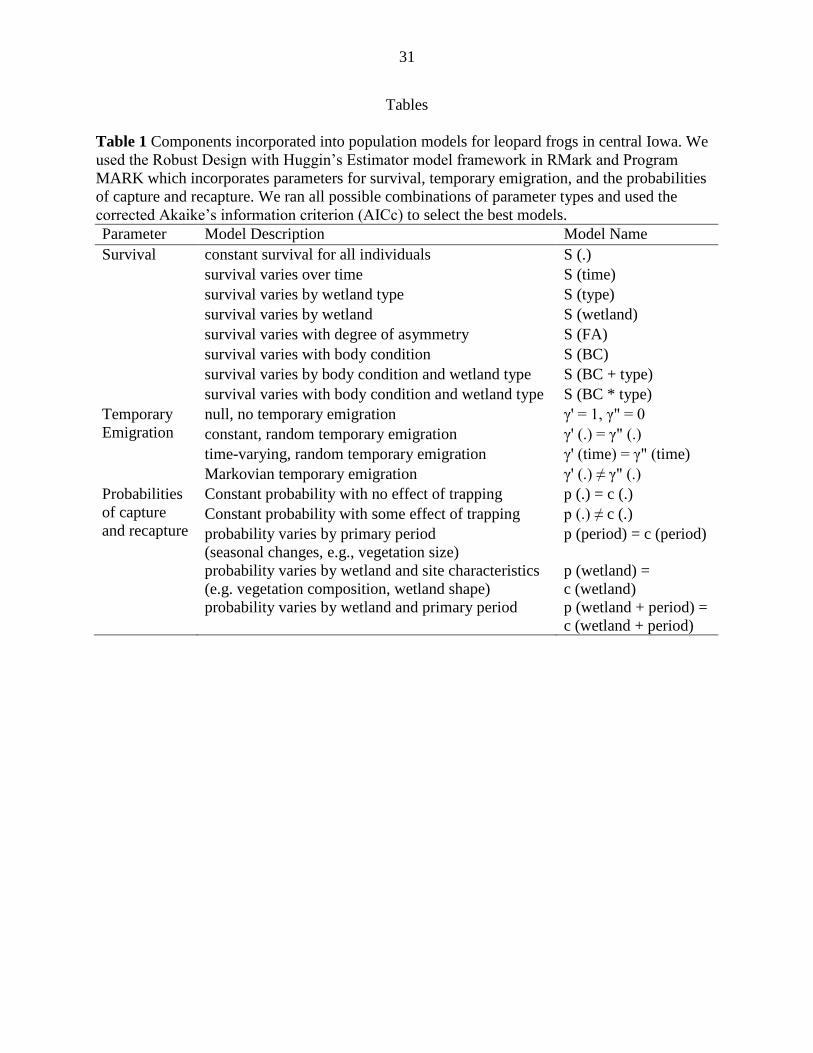
We included eight models for apparent survival (S; Table 1): constant survival (S (.));

time-varying survival (S (time)); survival varying by wetland type (i.e., CREP or reference, S

(type)); survival varying by wetland (S (wetland)); survival varying with degree of fluctuating

asymmetry (S(FA)); and survival varying with body condition (S(BC)). Because body condition

was different in CREP and reference wetlands, we also included combinations of body condition

and wetland type (S (BC * type) and S (BC + type)).

The robust design with Huggin’s estimator model incorporates two parameters relating to

temporary emigration from the study area (γ’ and γ”; Pollock, 1982; Kendall, 2014). We

included four types of temporary emigration models in our estimation (Table 1): no temporary

emigration (γ’ = 1 and γ” = 0); constant, random temporary emigration (γ'(.) = γ"(.)); time-

varying, random temporary emigration (γ'(time) = γ"(time)); and Markovian temporary

emigration (γ'(.) ≠ γ"(.); Kendall, 2014).

We included five models for the estimation of capture (p) and recapture (c) probabilities

(Table 1): probability of capture and recapture are equal and constant (no effect of trapping; p(.)

= c(.)); not equal and constant (some effect of trapping; p (.) ≠ c (.)); equal and change with each

primary period (p (period) = c (period)); equal and wetland dependent (p (wetland) = c

14

(wetland)); and equal and wetland and time dependent (p (wetland + period) = c (wetland +

period)). Allowing p and c to vary by primary period compensates for variation in vegetation

height and water level that naturally occurred throughout the season.

We calculated fluctuating asymmetry as the absolute value of the difference between

right and left limbs (Gallant & Teather, 2001; Appendix B). We measured the length of the

radioulna, thumb, femur, tibiofibula, and foot on each side of the body to the nearest 0.001mm;

each measurement was taken three times by one investigator (RAR) to minimize bias (St-Amour

et al., 2010). After measurements, frogs were released at their point of capture and observed until

moving normally (Green, 2001).

The tibiofibula best met the necessary criteria for exploring fluctuating asymmetry (as

outlined in Gallant & Teather 2001), and was the only limb included in further comparisons of

developmental stress between wetland types (Appendix B). We compared fluctuating asymmetry

in CREP and reference wetlands using an ANOVA with wetland type, sample year, age class,

and sex as explanatory variables and the absolute value of the differences between right and left

limbs as the response.

In 2012, 20 leopard frogs (N =5 from four wetlands) were sent to the USGS National

Wildlife Health Center in Madison, WI, USA to be necropsied and screened for gross

malformations and Bd and parasite infections. Amphibians were examined under a dissecting

microscope to identify lesions, malformations, or other abnormalities, and any parasites found

were keyed to genus.

We used the residuals from the regression of log(mass) on log(snout-to-urostyle-length)

for body condition of each frog (Băncilă et al., 2010). Positive residuals reflect heavier than

average individuals for their body length and can suggest increased food resources or less

15

environmental stress (Băncilă et al., 2010). We included adults as well as newly metamorphosed

individuals (fully absorbed tail) in the regression when comparing body condition among

wetlands, but included adults only when producing the covariates for modeling demographic

parameters. We compared the mean body condition of individuals at each wetland using a two-

way ANOVA with body condition as the response variable and wetland type, sample year, age

class, and sex as the explanatory variables.

Results

Environmental Characteristics

Environmental characteristics varied considerably among wetland types (MANOVA,

F=10.56, p <0.001; Appendix C, Table C1). The largest sources of variation in water chemistry

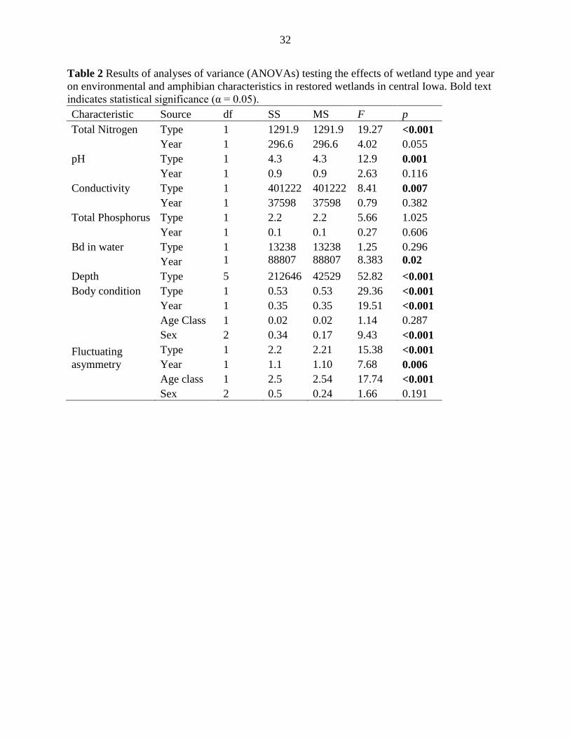
between CREP and reference wetlands were conductivity, pH, and total nitrogen (Table 2).

CREP wetlands were deeper and had higher nitrogen concentrations (Table 3; Figure 4). Overall,

Story CREP had the highest mean nitrogen concentration, while the three reference wetlands had

the lowest concentrations (Table 3). Differences in nitrogen concentrations between CREP and

reference wetlands were more distinct in 2013 than 2012 (2012: CREP: 9.3 mg/L, reference: 2.6

mg/L; 2013: CREP: 20.5 mg/L, reference: 2.8 mg/L). CREP wetlands were more alkaline than

reference wetlands (Figure 4).

In reference wetlands, pH ranged from 7.4-8.6, while the pH in CREP wetlands was

generally higher (7.4 – 10.2). Conversely, conductivity was higher in reference wetlands than in

CREP wetlands (Figure 4). Boone and Bob Pyle reference wetlands had the highest mean and

most variation in conductivity (Table 3). There were no differences in phosphorus concentrations

between CREP and reference wetlands.

16

The concentration of Bd zoospores in water samples varied between years. The mean

concentration of Bd zoospores in water samples was three times higher in reference wetlands

(309 ± 73.8) than CREP wetlands (110 ± 60.2) in 2012, but differences were less distinct in 2013

(Figure 4). Water samples from Boone reference wetland held the greatest concentration of

zoospores in both 2012 and 2013 (Table 3).

On average, CREP wetlands were twice as deep as reference wetlands (Table 3;

Appendix D, Figure D1). The mean depth in CREP wetlands ranged between 56 and 70 cm with

maximum depths between 158 and 240 cm, while the mean depths of reference wetlands were

shallower than 22 cm with maximum depths between 28 and 56 cm (Table 3). In 2012, the

Midwest experienced a drought, and all three reference wetlands dried up by mid-July, while the

CREP wetlands retained water (Table 3).

Fish were found in all three CREP wetlands, but only one reference wetland (Table 3).

Bullfrog choruses were observed in all three CREP wetlands. Although not detected in call

recordings, bullfrogs were encountered occasionally at reference wetlands.

Amphibian Characteristics

With the exception of bullfrogs, the amphibian assemblages were similar in the two

wetland types (Appendix A, Table A2). Every wetland had gray tree frogs (Hyla spp.), American

toads (Anaxyrus americanus) and chorus frogs (Pseudacris maculata) both years, while most had

leopard frogs and cricket frogs both years (Appendix A, Table A2). Leopard frog calls were

recorded at Marshall CREP in 2012 but leopard frogs were not detected visually in either 2012 or

2013.

We captured 25 frogs at CREP wetlands and 159 at reference wetlands in 2012. In 2013,

we captured 16 frogs at CREP sites and 21 frogs at reference sites (Appendix A, Table A3).

17

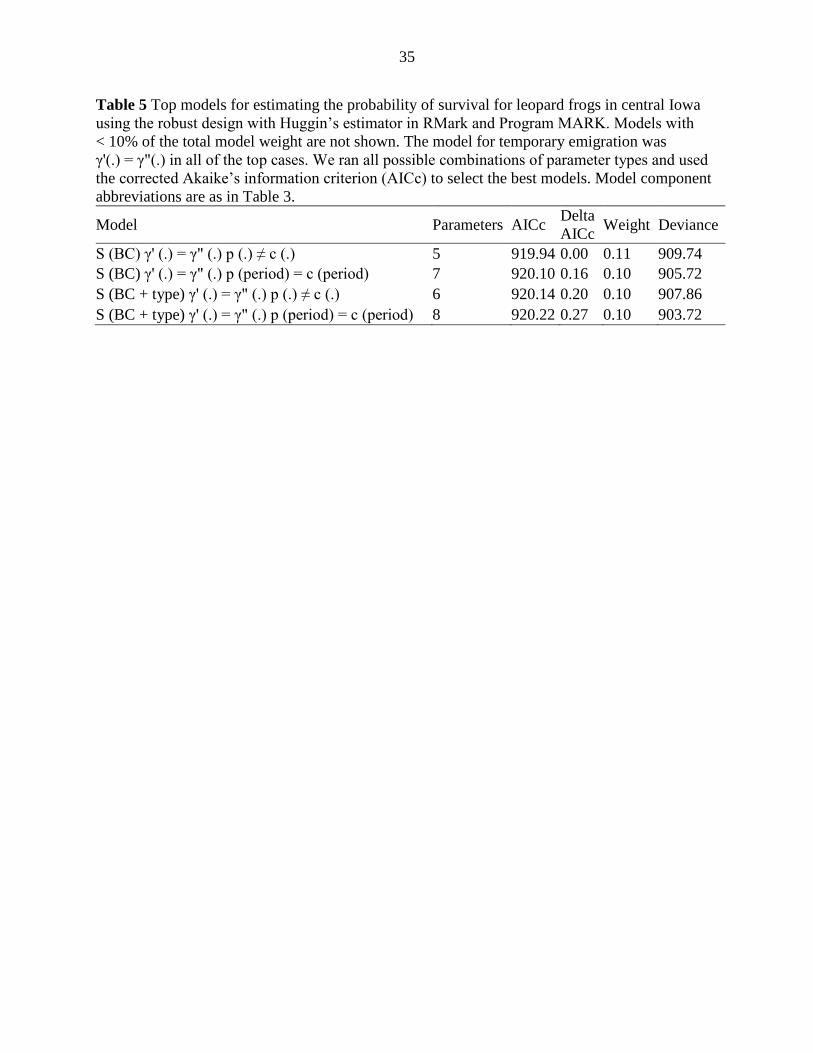
Model selection for the analysis of leopard frog demographics supported the inclusion of body

condition in estimating survival and to a lesser extent, wetland type (Table 5; full AIC table in

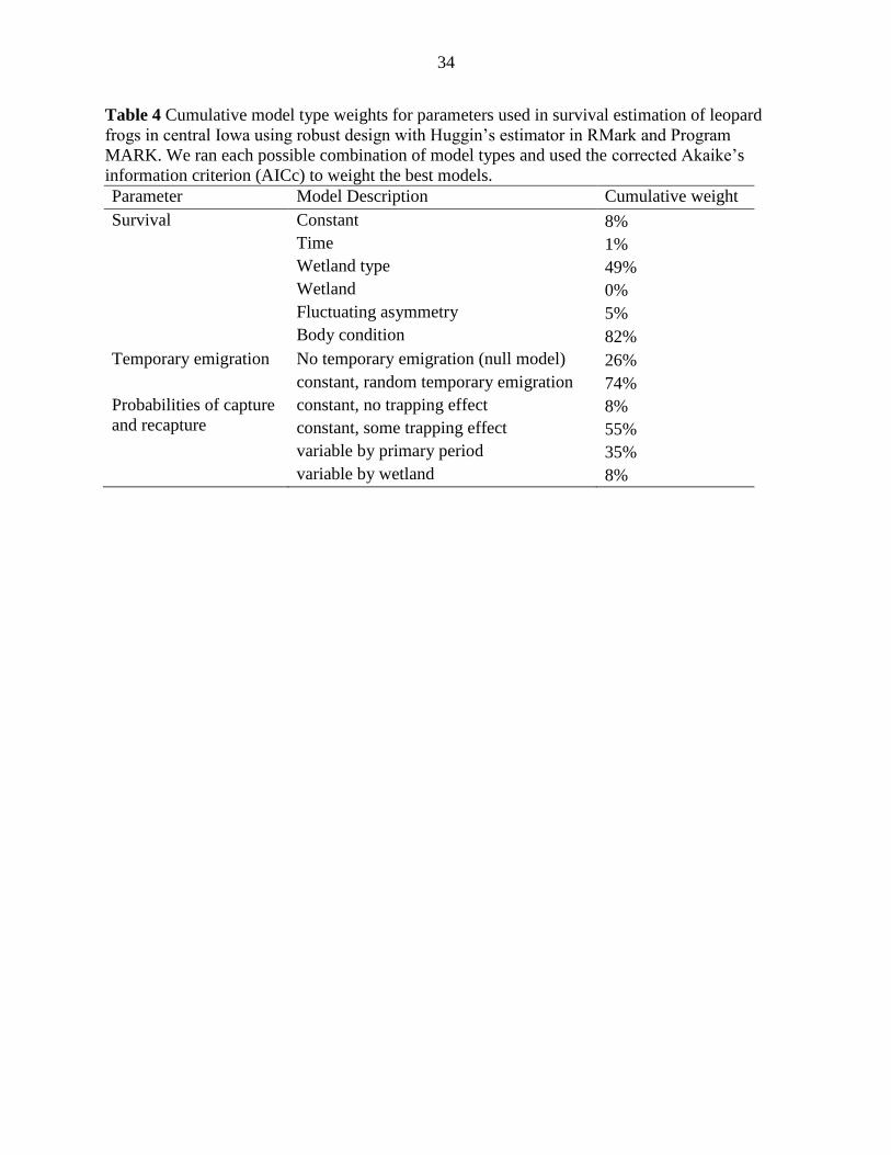
Appendix E). There was no support for fluctuating asymmetry, time, or wetland affecting

survival (cumulative model weights ≤ 5%; Table 4). Although models incorporating body

condition were highly ranked, it is unclear whether body condition is a significant covariate for

survival since the 95% confidence intervals surrounding the beta estimates for body condition

cross zero in nine of the top ten models (Table 6). There were no differences in model averaged

survival probabilities for CREP and reference wetlands: CREP: 80% (CI: 0.45-0.95); Reference:

66% (CI: 0.33-0.89; Appendix D, Figure D2).

The return rate of temporary emigrants (given by 1-γ’ and 1-γ”) were relatively low, so

there was a high probability of individuals leaving wetlands and not returning (γ’= 0.87 ± 0.12,

γ”= 0.61 ± 0.37). Models that incorporated constant, random temporary emigration accounted for

74% of the model weight compared to the null (no temporary emigration) models. Several

models, including all time-varying, random temporary emigration, all markovian temporary

emigration, and four time-varying survival models did not converge so were removed from the

model set.

Probabilities of capture and recapture that were constant but not equal to one another

received the most cumulative model weight (55%), followed by those that varied by primary

period (47%; Table 4). Probabilities of capture ranged from 12-22% (± 3-5%), while

probabilities of recapture ranged from 23- 33% (± 4-10%) and were not significantly different

among wetlands.

18

The size of adult leopard frog population varied among wetlands but did not vary

consistently within wetland types (Figure 5). In most wetlands, the estimated adult population

size decreased between May and June both years, although the population at Greene CREP

remained fairly consistent throughout the study. Additionally, populations were generally smaller

in 2013 than they were during the same month in 2012. Story CREP maintained the smallest

leopard frog population of all wetlands included in capture-recapture efforts.

Leopard frog metamorphs were observed in one reference and two CREP wetlands in

2012 and in all wetlands except Marshall CREP in 2013 (Table 3). In 2012, reference wetlands

had dried or were drying during peak metamorph emergence (Table 3).

All five leopard frogs collected from Story CREP had heavy trematode infections in the

main body cavity, but heavy infections were not detected in individuals collected elsewhere. One

intersex individual (with both a Bidder’s-like organ and testes) was collected from Bjorkboda

reference in 2012 (Appendix H).

Assessment of fluctuating asymmetry (average right - left side tibiofibula lengths)

suggested differences in developmental stress in frogs at CREP versus reference wetlands and

between years. Limb asymmetries were larger in adults than metamorphs (Metamorphs: CREP:

0.22 mm, REF: 0.28 mm), but there were no differences between sexes. Adult frogs in reference

wetlands had asymmetries nearly twice as large as those in CREP wetlands (Adults: CREP: 0.34

mm, REF: 0.51 mm, Figure 6). The mean difference in limb length was highest in Boone County

reference for both adults and metamorphs and was correlated positively with the concentration of

Bd zoospores in water in both years (Appendix C, Table C2).

Body condition analysis also revealed higher levels of developmental stress in reference

wetlands. Frogs in CREP wetlands were generally heavier than frogs of the same length in

19

reference wetlands (Figure 6). Body condition was highest at Greene CREP and lowest at Boone

reference and was correlated negatively with the number of Bd zoospores detected in water

samples (Appendix C, Table C2).

Discussion

Amphibian habitat quality differed in CREP and reference wetlands, but effects on

amphibians appear to be sub-lethal. There were differences in the total nitrogen concentrations,

pH, conductivity, and the abundance of Bd zoospores in water samples as well as substantial

differences in hydroperiod and mean depth among wetlands. Despite these differences in habitat

quality, there were few differences in amphibian assemblages between wetland types and no

discernible differences in leopard frog survival probabilities. Leopard frogs in reference wetlands

exhibited more developmental stress (i.e., decreased body condition and larger asymmetries)

than those in CREP wetlands, but neither fluctuating asymmetry nor body condition were clearly

related to survival.

Environmental Characteristics

CREP wetlands are designed to sequester 40-90% of the nitrogen that flows into them,

providing an ecosystem service (Iovanna et al., 2008), and as expected, nitrogen concentrations

were higher in CREP than in reference wetlands. Increased nitrogen concentrations can alter

food web structure and can change parasite-host relationships. For example, increases in

secondary host (snail) populations can increase the number of parasites (trematodes) in a

wetland, thus increasing the risk of parasitism for amphibians (Johnson et al., 2007). In line with

this scenario, we found that the wetland with the highest total nitrogen concentration in both

years also had the highest occurrence of trematode parasites and the smallest adult leopard frog

population in 2013.

20

CREP wetlands also had more alkaline pH than reference wetlands. High pH and high

water temperatures facilitate high concentrations of ammonia (Emerson et al., 1975; Thurston et

al., 1981). Low, ecologically relevant concentrations of ammonia can cause reduced survival,

higher rates of deformity, and decreased growth and development in tadpoles (Jofre & Karasov,

1999). Water was more conductive in reference wetlands, although species richness, which can

decline with increased conductivity (Hecnar & McCloskey 1996), was not different between

wetland types.

While CREP wetlands had generally poorer water quality, reference wetlands had higher

concentrations of Bd zoospores, especially in 2012. Seasonal drying of wetlands may reduce the

potential for Bd infection (Johnson et al., 2003) and after reference wetlands dried completely

(summer / fall 2012) we found that the number of zoospores in water samples was reduced by

more than 90%. Bd can have lethal and sub-lethal impacts by killing animals (Briggs et al.,

2010), reducing survival (Pilliod et al., 2010), altering interspecific competition, or increasing

hind limb asymmetry (Parris & Cornelius, 2004). Our data indicate that survival was not

compromised by Bd presence but the presence of Bd was correlated positively with

developmental stress.

CREP wetlands were deeper and retained water longer than reference wetlands in the

drought in 2012. CREP wetlands are designed to intercept more sub-surface flow than reference

wetlands and likely have a more consistent water supply, contributing to their longer

hydroperiods. Longer hydroperiods allow for more denitrification, but also facilitate predatory

species such as bullfrogs and fish that can reduce amphibian species richness, abundance, and

breeding success (Boone et al., 2004; Boone et al., 2007). Bullfrogs, which are not native to

21

central Iowa, are voracious predators that eat fish, birds, and other frogs and are also vectors for

Bd (Lannoo, 1996, Casper & Hendricks, 2005).

Bullfrogs and fish tended to be present in CREP wetlands and absent from reference

wetlands, although there was variation among years. The fish species detected eat a variety of

prey, potentially including all life stages of frogs (Carlander, 1969; 1977). While body size and

mouth gape limitations probably prevent bluegills from preying on adult frogs and likely prevent

fathead minnows from preying on tadpoles and adults, predation on eggs is possible from all

species (Carlander, 1969; 1977). Bullfrog tadpoles generally take two seasons to metamorphose

and must overwinter in wetlands, so, like fish; they require deeper wetlands that will remain at

least partially unfrozen throughout the winter (Casper & Hendricks, 2005). CREP wetlands are

restored as shallow-water emergent wetlands designed to have 75% of the wetland pool < 1 m

deep, however all of the CREP wetlands in this study were > 1.5 m deep at their deepest point

(IDALS, 2009; 2013). At this depth, there is potential for long hydroperiods and portions of the

wetland to remain unfrozen. Such characteristics facilitate the presence of fish and bullfrogs and

reduce the quality of the habitat for amphibians (Porej & Hetherington, 2005; Walston & Mullin,

2007; Shulse et al., 2010). Conversely, having deeper, unfrozen pools available during the winter

may also facilitate the presence of some amphibian species. For example, leopard frogs bury

themselves in the sediments in deep, oxygen rich pools over the winter (Rorabaugh, 2005). We

observed very few leopard frogs and no successful leopard frog reproduction at Marshall CREP,

which had bullfrogs and the greatest diversity of fish. This suggests that at this wetland, the

benefit of increased leopard frog habitat availability was outweighed by increased predation.

Deeper areas in CREP wetlands may provide important resources for some species that

might otherwise be unavailable or limited in agricultural landscapes. The availability of wetlands

22

with a variety of hydroperiods is likely to be beneficial to the persistence of amphibian

populations in such an altered landscape, with deep wetlands providing overwintering sites and

refuge during drought, and shallower wetlands providing refuge from predators (McCaffery

2014). Our study underscores the importance of variety in wetland hydroperiods. Between July

2012 and February 2013, there were 30 weeks when >25% of the Midwest experienced “severe

drought,” whereas the next year, there were only five weeks when 10% or more of the Midwest

experienced “severe drought” (NDMC et al., 2014). All of our reference wetlands dried between

June and July in 2012, when leopard frog metamorphs were emerging from wetlands.

There are advantages for amphibians in the design of CREP wetlands. These wetlands

have built-in flow control structures to allow for mechanical water level draw-downs (IDALS,

2013). Drawdowns could reduce or eliminate bullfrogs and fish, and complete drawdowns

(drying) could reduce the effect of Bd (Johnson et al., 2003; Rowe & Garcia 2014). Drawdowns,

while temporarily reducing the processing of nitrate by the wetland, consolidate sediments,

increase water clarity and facilitate colonization and establishment of emergent vegetation which

benefits denitrification (Van der Valk & Davis, 1978; IDALS, 2013).

Amphibian Characteristics

Despite their differences in environmental characteristics, there were no significant

differences in the probability of survival for adult leopard frogs between wetland types. The

average monthly survival probability for adults across both wetland types was 74.5%, which if

extrapolated would yield an annual survival rate of 3%. While a survival rate estimated in the

summer and extrapolated over the entire year is only a crude approximation of true annual

survival, we are unaware of any published estimates of adult leopard frog annual survival

probabilities in free-living populations for comparison. Female adult leopard frogs typically

23

mature in their third activity season (age 2; Dodd, 2013). In Quebec, Canada, wild individuals

collected for osteoanalysis showed large growth rates between their first and second years, and

individuals more than 3 years old were relatively scarce (Leclair Jr & Castanet, 1987). Leopard

frogs generally have a short lifespan and a life history strategy that favors explosive

reproduction. Because central Iowa is a heavily modified landscape in which much of the

historical habitat has been lost and remaining habitat is subject to nutrient and pesticide

contamination, the 3% annual survival probability extrapolated from our monthly estimate may

not be surprising, especially considering the drought experienced across the Midwest in 2012. A

full understanding of potential population persistence is not yet possible as we did not assess

recruitment, but future capture-recapture studies in similar landscapes could contribute greatly to

our knowledge.

Survival models that incorporated body condition had the highest cumulative weight;

however the betas used to estimate the top ten models were not significant at the 95% confidence

level (Appendix A, Table A4). Additionally, since there was such variation in the number and

body condition of frogs captured at each wetland (Appendix D, Figure D3), we feel that we

cannot make any reasonable inference about the importance of body condition for survival.

As expected, populations of adult frogs tended to decrease from May to June, as individuals

finished breeding and returned to the uplands. Since populations were smaller in 2013 than 2012,

it is possible that individuals perished or permanently emigrated due to the drought. Further

study could elucidate whether individuals eventually returned to the wetlands where they were

first marked. Since the drought persisted into the beginning of the breeding season in 2013,

perhaps frogs elected to breed elsewhere, where water was more available.

24

Overall, CREP and reference wetlands offer different qualities of amphibian habitat.

CREP wetlands were characterized by higher nitrogen concentrations, more alkaline pH, slightly

longer hydroperiods, and greater depths. Differences in structural characteristics may contribute

to the increased prevalence of non-native bullfrogs and fish, while high nitrogen concentrations

may increase the risk of trematode parasitism for resident amphibians. Unfortunately, these

physical characteristics are central to the primary nitrogen removal functions of CREP wetlands,

so cannot be easily avoided. Mechanical drawdowns, which are already recommended on an as-

needed basis for emergent vegetation management in CREP wetlands, could have an added

benefit of reducing the impact of predators such as bullfrogs and fish on other amphibian species.

Reference wetlands had higher concentrations of Bd zoospores and a higher incidence of

developmental stress, but overall there were few differences in the composition of the amphibian

assemblage, or in the population sizes and survival probabilities of leopard frogs between

wetland types. CREP and reference wetlands provide important components of habitat to

amphibians in central Iowa. Maintaining some relatively predator-free wetlands within the larger

complex of wetlands with a variety of hydroperiods appears to be important for the long term

persistence of amphibians in this landscape, especially in light of increasing variability in rainfall

due to climate change.

Acknowledgements

This project was funded by the Fort Collins Science Center as a part of ongoing technical

assistance given to the Farm Service Agency to assess Iowa CREP wetlands and the USGS

Amphibian Research and Monitoring Initiative (ARMI). We owe thanks to a number of people

including T. Grant, D. Otis, D. Green, D. Cook, J. Niemi, S. Richmond, M. Lechtenberg, the

field technicians, and the army of volunteers and that made this study possible. We would

25

especially like to thank J. Oberheim-Vorwald, K. Edmunds, L. Truong, J. Harmon, and K. Flood

as well as all the landowners that allowed us access to their wetlands. Exact wetland locations

are proprietary, and we obtained written permission for access to wetlands from all landowners

and public land managers prior to the start of sampling. This study was performed under the

auspices of Iowa State University Institutional Animal Care and Use Committee (IACUC)

protocol # 3-12-7324-D. Use of trade, product, or firm names is descriptive and does not imply

endorsement by the U.S. Government.

Literature Cited

Băncilă, R. I., T. Hartel, R. Plăiaşu, J. Smets and D. Cogălniceanu. 2010. Comparing three body

condition indices in amphibians: a case study of yellow-bellied toad Bombina variegata.

Amphibia-Reptilia, 31:558-562.

Beaupre, S., E. Jacobson, H. Lillywhite and K. Zamudio. 2004. Guidelines for use of live

amphibians and reptiles in field and laboratory research. A publication of the American

Society of Ichthyologists and Herpetologists, approved by board of Governors.

Blanar, C. A., K. R. Munkittrick, J. Houlahan, D. L. MacLatchy and D. J. Marcogliese. 2009.

Pollution and parasitism in aquatic animals: A meta-analysis of effect size. Aquatic

Toxicology, 93:18-28.

Bogue, A. G. 1963. From prairie to corn belt: Farming on the Illinois and Iowa prairies in the

nineteenth century. Iowa State University Press, Ames, IA, USA.

Boone, M. D. and S. M. James. 2003. Interactions of an insecticide, herbicide, and natural

stressors in amphibian community mesocosms. Ecological Applications, 13:829-841.

Boone, M. D., E. E. Little and R. D. Semlitsch. 2004. Overwintered bullfrog tadpoles negatively

affect salamanders and anurans in native amphibian communities. Copeia, 3:683-690.

Boone, M. D., R. D. Semlitsch, E. E. Little and M. C. Doyle. 2007. Multiple stressors in

amphibian communities: effects of chemical contamination, bullfrogs, and fish. Ecological

Applications, 17:291-301.

Briggs, C. J., R. A. Knapp and V. T. Vredenburg. 2010. Enzootic and epizootic dynamics of the

chytrid fungal pathogen of amphibians. Proceedings of the National Academy of Sciences of

the United States of America, 107:9695-9700.

26

Carlander, K. D. 1969. Handbook of Freshwater Fishery Biology. Iowa State University Press,

Ames, IA, USA.

Carlander, K. D. 1977. Handbook of Freshwater Fishery Biology. Iowa State University Press,

Ames, IA, USA.

Casper, G. S. and R. Hendricks. 2005. Rana catesbeiana. In M. Lannoo (ed.), Amphibian

Declines. University of California Press, Berkeley, CA, USA.

Collins, J. P. and A. Storfer. 2003. Global amphibian declines: sorting the hypotheses. Diversity

and Distributions, 9:89-98.

Cushman, S. A. 2006. Effects of habitat loss and fragmentation on amphibians: A review and

prospectus. Biological Conservation, 128:231-240.

Dias, P. C. 1996. Sources and sinks in population biology. Trends in Ecology and Evolution

11:326-330.

Dodd, C. K. 2013. Frogs of the United States and Canada, 2-vol. set. Johns Hopkins University

Press.

Doherty, P. F., G. C. White and K. P. Burnham. 2012. Comparison of model building and

selection strategies. Journal of Ornithology, 152:317-323.

Emerson, K., R. C. Russo, R. E. Lund and R. V. Thurston. 1975. Aqueous ammonia equilibrium

calculations: effect of pH and temperature. Journal of the Fisheries Board of Canada,

32:2379-2383.

Ferner, J. 2007. A review of marking and individual recognition techniques for amphibian and

reptiles. Herpetological Circular 35. Society for the Study of Amphibians and Reptiles.

Atlanta, USA.

Gallant, N. and K. Teather. 2001. Differences in size, pigmentation, and fluctuating asymmetry

in stressed and nonstressed northern leopard frogs (Rana pipiens). Ecoscience, 8:430-436.

Green, D. E. 2001. Anesthesia of amphibians in the field. United States Geological Survey,

Madison, WI, USA.

Groner, M. L. and R. A. Relyea. 2011. A tale of two pesticides: How common insecticides affect

aquatic communities. Freshwater Biology, 56:2391-2404.

Hecnar, S. J. 1995. Acute and chronic toxicity of ammonium-nitrate fertilizer to amphibians

from Southern Ontario. Environmental Toxicology and Chemistry, 14:2131-2137.

Hecnar, S. J. and R. T. MCloskey. 1996. Amphibian species richness and distribution in relation

to pond water chemistry in south-western Ontario, Canada. Freshwater Biology, 36:7-15.

27

Hubert, W. A., K. L. Pope and J. M. Dettmers. 2012. Passive capture techniques. p. 223-265. In

A. V. Zale, D. L. Parrish and T. M. Sutton (eds.), Fisheries Techniques. American Fisheries

Society, Bethesda, MD, USA.

IDALS. 2009. Landowner guide to CREP. Iowa Department of Agriculture and Land

Stewardship.

IDALS. 2013. Iowa Conservation Reserve Enhancement Program (CREP) landowner guide to

operation and maintenance. Iowa Department of Agriculture and Land Stewardship.

IDNR. 2006. Iowa Wildlife Action Plan. Iowa Department of Natural Resources.

Iovanna, R., S. Hyberg and W. Crumpton. 2008. Treatment wetlands: Cost-effective practice for

intercepting nitrate before it reaches and adversely impacts surface waters. Journal of Soil

and Water Conservation, 63:14A-15A.

Jofre, M. B. and W. H. Karasov. 1999. Direct effect of ammonia on three species of North

American anuran amphibians. Environmental Toxicology and Chemistry, 18:1806-1812.

Johnson, M. L., L. Berger, L. Philips and R. Speare. 2003. Fungicidal effects of chemical

disinfectants, UV light, desiccation and heat on the amphibian chytrid Batrachochytrium

dendrobatidis. Diseases of Aquatic Organisms, 57:255-260.

Johnson, P. T. J., J. M. Chase, K. L. Dosch, R. B. Hartson, J. A. Gross, D. J. Larson, D. R.

Sutherland and S. R. Carpenter. 2007. Aquatic eutrophication promotes pathogenic infection

in amphibians. Proceedings of the National Academy of Sciences of the United States of

America, 104:15781-15786.

Kendall, W. 2014. The ‘robust design’. p. 15-01. In E. Cooch and G. C. White (eds.), Program

MARK:‘A gentle introduction.

Kendall, W. L. and J. D. Nichols. 1995. On the use of secondary capture-recapture samples to

estimate temporary emigration and breeding proportions. Journal of Applied Statistics,

22:751-762.

Kirshtein, J. D., C. W. Anderson, J. S. Wood, J. E. Longcore and M. A. Voytek. 2007.

Quantitative PCR detection of Batrachochytrium dendrobatidis DNA from sediments and

water. Diseases of Aquatic Organisms, 77:11.

Knutson, M. G., W. B. Richardson, D. M. Reineke, B. R. Gray, J. R. Parmelee and S. E. Weick.

2004. Agricultural ponds support amphibian populations. Ecological Applications, 14:669-

684.

28

Laake, J. 2013. RMark: An R interface for analysis of capture-recapture data with MARK.

Alaska Fisheries Science Center, NOAA National Marine Fisheries Service, Seattle, WA

USA.

Lannoo, M. J. 1996. Okoboji wetlands: a lesson in natural history. University of Iowa Press.

Iowa City, IA, USA.

Lannoo, M. J. 1998. Status and conservation of midwestern amphibians. University of Iowa

Press. Iowa City, IA, USA.

Leclair Jr, R. and J. Castanet. 1987. A skeletochronological assessment of age and growth in the

frog Rana pipiens Schreber (Amphibia, Anura) from southwestern Quebec. Copeia:361-369.

McCaffery, R. M., L. A. Eby, B. A. Maxell and P. S. Corn. 2014. Breeding site heterogeneity

reduces variability in frog recruitment and population dynamics. Biological Conservation,

170:169-176.

Miller, B. A., W. G. Crumpton and A. G. van der Valk. 2009. Spatial distribution of historical

wetland classes on the Des Moines Lobe, Iowa. Wetlands, 29:1146-1152.

NDMC, USDA and NOAA. 2014. United States drought monitor archives. National Drought

Mitigation Center, U.S. Department of Agriculture, National Oceanic and Atmospheric

Administration.

O'Neal, B. J., E. J. Heske and J. D. Stafford. 2008. Waterbird response to wetlands restored

through the Conservation Reserve Enhancement Program. The Journal of Wildlife

Management, 72:654-664.

Patton, C. J. and J. R. Kryskalla. 2003. Methods of analysis by the US Geological Survey

National Water Quality Laboratory: Evaluation of alkaline persulfate digestion as an

alternative to kjeldahl digestion for determination of total and dissolved nitrogen and

phosphorus in water. US Department of the Interior, US Geological Survey.

Parris, M. J. and T. O. Cornelius. 2004. Fungal pathogen causes competitive and developmental

stress in larval amphibian communities. Ecology, 85:3385-3395.

Pilliod, D. S., E. Muths, R. D. Scherer, P. E. Bartelt, P. S. Corn, B. R. Hossack, B. A. Lambert,

R. Mccaffery and C. Gaughan. 2010. Effects of amphibian chytrid fungus on individual

survival probability in wild boreal toads. Conservation Biology, 24:1259-1267.

Pollock, K. H. 1982. A capture-recapture design robust to unequal probability of capture. The

Journal of Wildlife Management:752-757.

Porej, D. and T. E. Hetherington. 2005. Designing wetlands for amphibians: the importance of

predatory fish and shallow littoral zones in structuring of amphibian communities. Wetlands

Ecology and Management, 13:445-455.

29

Pulliam, H. R. 1988. Sources, sinks and population regulation. The American Naturalist,

132:652-661.

Rohr, J. R., T. R. Raffel, S. K. Sessions and P. J. Hudson. 2008. Understanding the net effects of

pesticides on amphibian trematode infections. Ecological Applications, 18:1743-1753.

Rorabaugh, J. C. 2005. Rana pipiens. In M. Lannoo (ed.), Amphibian Declines. University of

California Press, Berkeley, CA, USA.

Rowe, J. C. and T. S. Garcia. 2014. Impacts of wetland restoration efforts on an amphibian

assemblage in a multi-invader community. Wetlands, 34:141-153.

Shulse, C. D., R. D. Semlitsch, K. M. Trauth and A. D. Williams. 2010. Influences of design and

landscape placement parameters on amphibian abundance in constructed wetlands. Wetlands,

30:915-928.

Smith, P. N., G. P. Cobb, C. Godard-Codding, D. Hoff, S. T. McMurry, T. R. Rainwater and K.

D. Reynolds. 2007. Contaminant exposure in terrestrial vertebrates. Environmental Pollution,

150:41-64.

St-Amour, V., T. W. Garner, A. I. Schulte-Hostedde and D. Lesbarreres. 2010. Effects of two

amphibian pathogens on the developmental stability of green frogs. Conservation Biology :

the journal of the Society for Conservation Biology, 24:788-794.

Thurston, R. V., R. C. Russo and G. Vinogradov. 1981. Ammonia toxicity to fishes. Effect of pH

on the toxicity of the un-ionized ammonia species. Environmental Science & Technology,

15:837-840.

USFWS. 2002. National Wetlands Inventory. U.S. Department of the Interior, U.S. Fish and

Wildlife Service, Washington, D.C.

Van der Valk, A. and C. Davis. 1978. The role of seed banks in the vegetation dynamics of

prairie glacial marshes. Ecology:322-335.

Waddle, J. H., T. F. Thigpen and B. M. Glorioso. 2009. Efiicacy of automatic vocalization

recognition software for anuran monitoring. Herpetological Conservation and Biology,

4:384-388.

Wake, D. B. and V. T. Vredenburg. 2008. Are we in the midst of the sixth mass extinction? A

view from the world of amphibians. Proceedings of the National Academy of Sciences of the

United States of America, 105:11466-11473.

Walston, L. J. and S. J. Mullin. 2007. Responses of a pond-breeding amphibian community to

the experimental removal of predatory fish. American Midland Naturalist, 157:63-73.

30

White, G. C. and K. P. Burnham. 1999. Program MARK: survival estimation from populations

of marked animals. Bird Study, 46:120-139.

Whitney, G. C. 1994. From coastal wilderness to fruited plain: a history of environmental change

in temperate North America, 1500 to the present. Cambridge University Press, Cambridge,

UK.

31

Tables

Table 1 Components incorporated into population models for leopard frogs in central Iowa. We

used the Robust Design with Huggin’s Estimator model framework in RMark and Program

MARK which incorporates parameters for survival, temporary emigration, and the probabilities

of capture and recapture. We ran all possible combinations of parameter types and used the

corrected Akaike’s information criterion (AICc) to select the best models.

Parameter Model Description Model Name

Survival constant survival for all individuals S (.)

survival varies over time S (time)

survival varies by wetland type S (type)

survival varies by wetland S (wetland)

survival varies with degree of asymmetry S (FA)

survival varies with body condition S (BC)

survival varies by body condition and wetland type S (BC + type)

survival varies with body condition and wetland type S (BC * type)

Temporary

Emigration

null, no temporary emigration γ' = 1, γ" = 0

constant, random temporary emigration γ' (.) = γ" (.)

time-varying, random temporary emigration γ' (time) = γ" (time)

Markovian temporary emigration γ' (.) ≠ γ" (.)

Probabilities

of capture

and recapture

Constant probability with no effect of trapping p (.) = c (.)

Constant probability with some effect of trapping p (.) ≠ c (.)

probability varies by primary period

(seasonal changes, e.g., vegetation size)

p (period) = c (period)

probability varies by wetland and site characteristics

(e.g. vegetation composition, wetland shape)

p (wetland) =

c (wetland)

probability varies by wetland and primary period p (wetland + period) =

c (wetland + period)

32

Table 2 Results of analyses of variance (ANOVAs) testing the effects of wetland type and year

on environmental and amphibian characteristics in restored wetlands in central Iowa. Bold text

indicates statistical significance (α = 0.05).

Characteristic Source df SS MS F p

Total Nitrogen Type 1 1291.9 1291.9 19.27 <0.001

Year 1 296.6 296.6 4.02 0.055

pH Type 1 4.3 4.3 12.9 0.001

Year 1 0.9 0.9 2.63 0.116

Conductivity Type 1 401222 401222 8.41 0.007

Year 1 37598 37598 0.79 0.382

Total Phosphorus Type 1 2.2 2.2 5.66 1.025

Year 1 0.1 0.1 0.27 0.606

Bd in water Type 1 13238 13238 1.25 0.296

Year 1 88807 88807 8.383 0.02

Depth Type 5 212646 42529 52.82 <0.001

Body condition Type 1 0.53 0.53 29.36 <0.001

Year 1 0.35 0.35 19.51 <0.001

Age Class 1 0.02 0.02 1.14 0.287

Sex 2 0.34 0.17 9.43 <0.001

Fluctuating

asymmetry

Type 1 2.2 2.21 15.38 <0.001

Year 1 1.1 1.10 7.68 0.006

Age class 1 2.5 2.54 17.74 <0.001

Sex 2 0.5 0.24 1.66 0.191

33

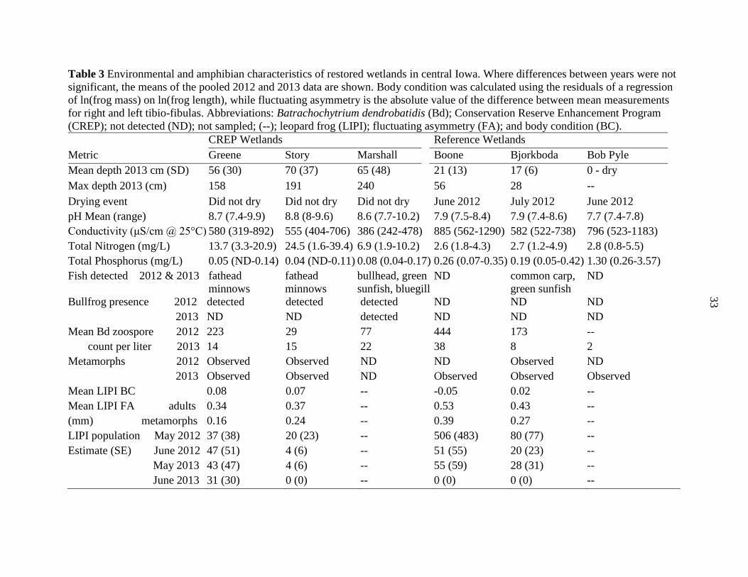
Table 3 Environmental and amphibian characteristics of restored wetlands in central Iowa. Where differences between years were not

significant, the means of the pooled 2012 and 2013 data are shown. Body condition was calculated using the residuals of a regression

of ln(frog mass) on ln(frog length), while fluctuating asymmetry is the absolute value of the difference between mean measurements

for right and left tibio-fibulas. Abbreviations: Batrachochytrium dendrobatidis (Bd); Conservation Reserve Enhancement Program

(CREP); not detected (ND); not sampled; (--); leopard frog (LIPI); fluctuating asymmetry (FA); and body condition (BC).

CREP Wetlands Reference Wetlands

Metric Greene Story Marshall Boone Bjorkboda Bob Pyle

Mean depth 2013 cm (SD) 56 (30) 70 (37) 65 (48) 21 (13) 17 (6) 0 - dry

Max depth 2013 (cm) 158 191 240 56 28 --

Drying event Did not dry Did not dry Did not dry June 2012 July 2012 June 2012

pH Mean (range) 8.7 (7.4-9.9) 8.8 (8-9.6) 8.6 (7.7-10.2) 7.9 (7.5-8.4) 7.9 (7.4-8.6) 7.7 (7.4-7.8)

Conductivity (μS/cm @ 25°C) 580 (319-892) 555 (404-706) 386 (242-478) 885 (562-1290) 582 (522-738) 796 (523-1183)

Total Nitrogen (mg/L) 13.7 (3.3-20.9) 24.5 (1.6-39.4) 6.9 (1.9-10.2) 2.6 (1.8-4.3) 2.7 (1.2-4.9) 2.8 (0.8-5.5)

Total Phosphorus (mg/L) 0.05 (ND-0.14) 0.04 (ND-0.11) 0.08 (0.04-0.17) 0.26 (0.07-0.35) 0.19 (0.05-0.42) 1.30 (0.26-3.57)

Fish detected 2012 & 2013 fathead

minnows

fathead

minnows

bullhead, green

sunfish, bluegill

ND common carp,

green sunfish

ND

Bullfrog presence 2012 detected detected detected ND ND ND

2013 ND ND detected ND ND ND

Mean Bd zoospore 2012 223 29 77 444 173 --

count per liter 2013 14 15 22 38 8 2

Metamorphs 2012 Observed Observed ND ND Observed ND

2013 Observed Observed ND Observed Observed Observed

Mean LIPI BC 0.08 0.07 -- -0.05 0.02 --

Mean LIPI FA adults 0.34 0.37 -- 0.53 0.43 --

(mm) metamorphs 0.16 0.24 -- 0.39 0.27 --

LIPI population May 2012 37 (38) 20 (23) -- 506 (483) 80 (77) --

Estimate (SE) June 2012 47 (51) 4 (6) -- 51 (55) 20 (23) --

May 2013 43 (47) 4 (6) -- 55 (59) 28 (31) --

June 2013 31 (30) 0 (0) -- 0 (0) 0 (0) --

33

34

Table 4 Cumulative model type weights for parameters used in survival estimation of leopard

frogs in central Iowa using robust design with Huggin’s estimator in RMark and Program

MARK. We ran each possible combination of model types and used the corrected Akaike’s

information criterion (AICc) to weight the best models.

Parameter Model Description Cumulative weight

Survival Constant 8%

Time 1%

Wetland type 49%

Wetland 0%

Fluctuating asymmetry 5%

Body condition 82%

Temporary emigration No temporary emigration (null model) 26%

constant, random temporary emigration 74%

Probabilities of capture

and recapture

constant, no trapping effect 8%

constant, some trapping effect 55%

variable by primary period 35%

variable by wetland 8%

35

Table 5 Top models for estimating the probability of survival for leopard frogs in central Iowa

using the robust design with Huggin’s estimator in RMark and Program MARK. Models with

< 10% of the total model weight are not shown. The model for temporary emigration was

γ'(.) = γ"(.) in all of the top cases. We ran all possible combinations of parameter types and used

the corrected Akaike’s information criterion (AICc) to select the best models. Model component

abbreviations are as in Table 3.

Model Parameters AICc Delta

AICc Weight Deviance

S (BC) γ' (.) = γ" (.) p (.) ≠ c (.) 5 919.94 0.00 0.11 909.74

S (BC) γ' (.) = γ" (.) p (period) = c (period) 7 920.10 0.16 0.10 905.72

S (BC + type) γ' (.) = γ" (.) p (.) ≠ c (.) 6 920.14 0.20 0.10 907.86

S (BC + type) γ' (.) = γ" (.) p (period) = c (period) 8 920.22 0.27 0.10 903.72

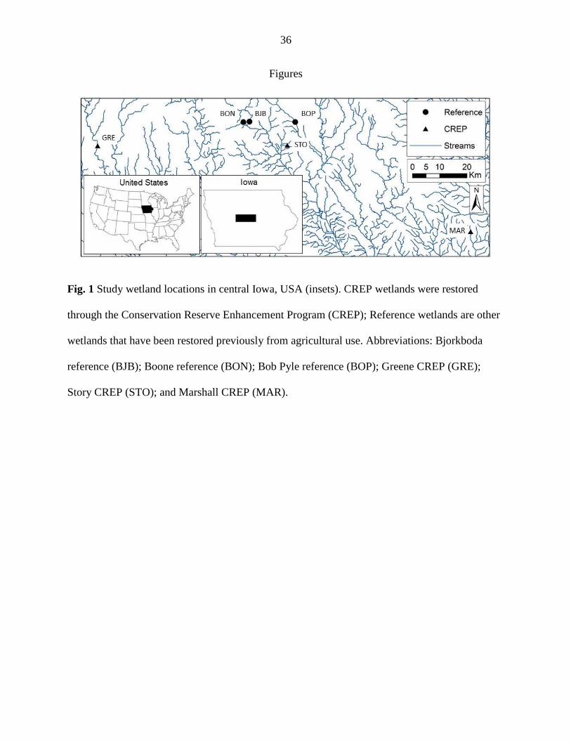
36

Figures

Fig. 1 Study wetland locations in central Iowa, USA (insets). CREP wetlands were restored

through the Conservation Reserve Enhancement Program (CREP); Reference wetlands are other

wetlands that have been restored previously from agricultural use. Abbreviations: Bjorkboda

reference (BJB); Boone reference (BON); Bob Pyle reference (BOP); Greene CREP (GRE);

Story CREP (STO); and Marshall CREP (MAR).

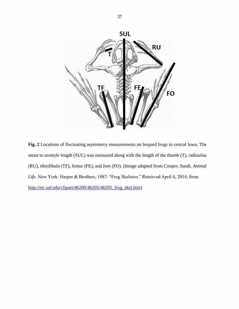
37

Fig. 2 Locations of fluctuating asymmetry measurements on leopard frogs in central Iowa. The

snout to urostyle length (SUL) was measured along with the length of the thumb (T), radioulna

(RU), tibiofibula (TF), femur (FE), and foot (FO). (Image adapted from Cooper, Sarah. Animal

Life. New York: Harper & Brothers, 1887. “Frog Skeleton.” Retrieved April 4, 2014, from

http://etc.usf.edu/clipart/46200/46205/46205_frog_skel.htm)

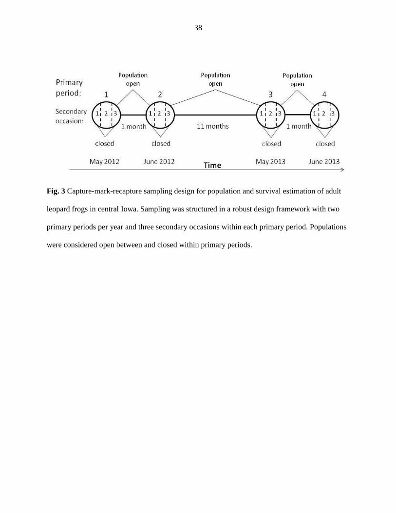
38

Fig. 3 Capture-mark-recapture sampling design for population and survival estimation of adult

leopard frogs in central Iowa. Sampling was structured in a robust design framework with two

primary periods per year and three secondary occasions within each primary period. Populations

were considered open between and closed within primary periods.

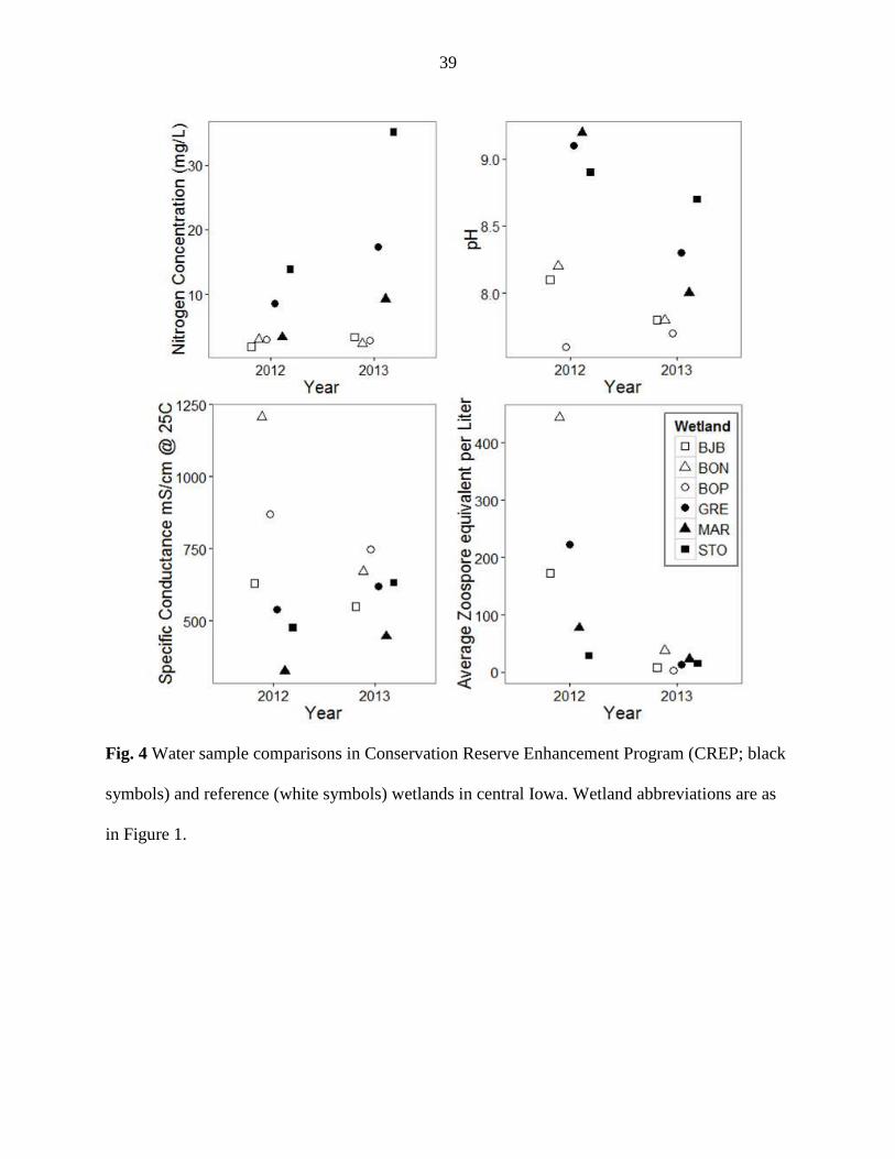
39

Fig. 4 Water sample comparisons in Conservation Reserve Enhancement Program (CREP; black

symbols) and reference (white symbols) wetlands in central Iowa. Wetland abbreviations are as

in Figure 1.

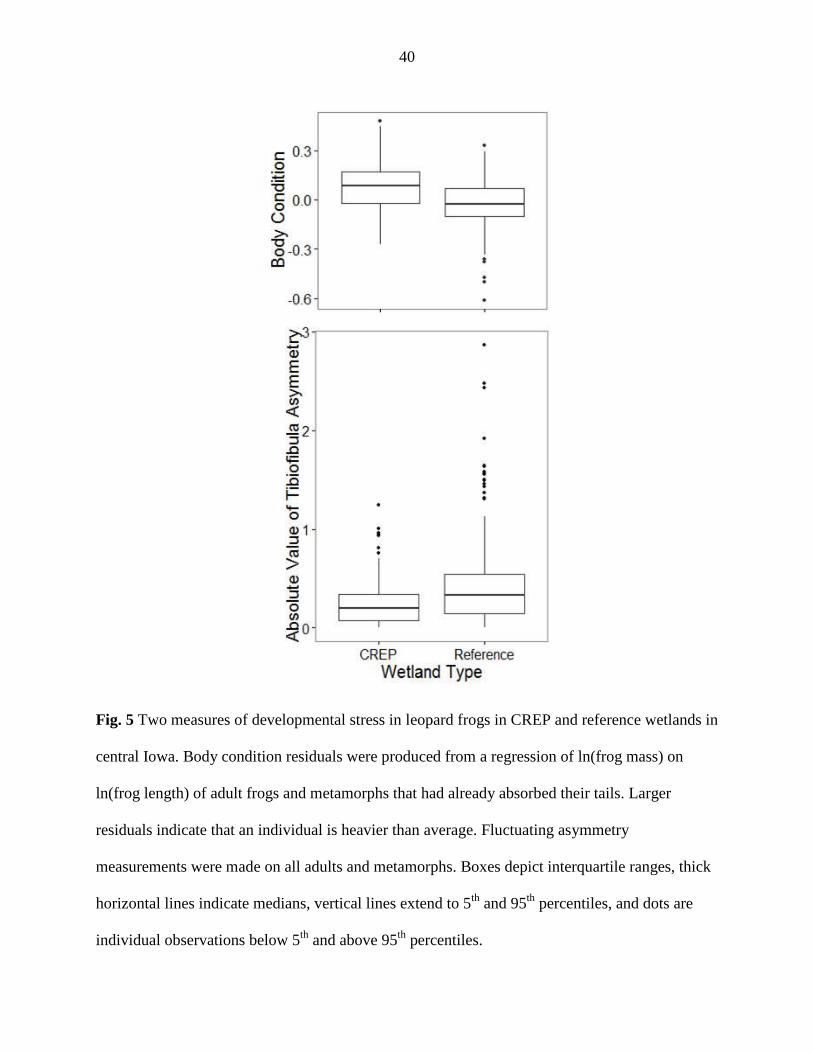
40

Fig. 5 Two measures of developmental stress in leopard frogs in CREP and reference wetlands in

central Iowa. Body condition residuals were produced from a regression of ln(frog mass) on

ln(frog length) of adult frogs and metamorphs that had already absorbed their tails. Larger

residuals indicate that an individual is heavier than average. Fluctuating asymmetry

measurements were made on all adults and metamorphs. Boxes depict interquartile ranges, thick

horizontal lines indicate medians, vertical lines extend to 5th

and 95th

percentiles, and dots are

individual observations below 5th

and above 95th

percentiles.

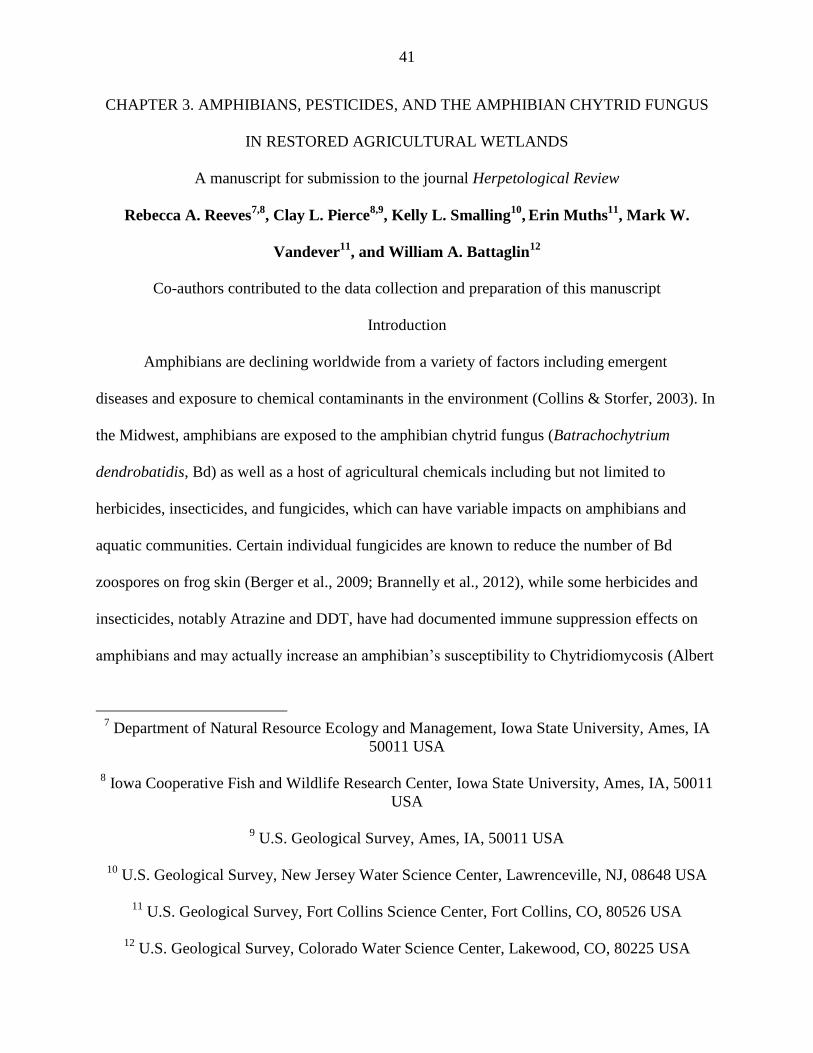
41

CHAPTER 3. AMPHIBIANS, PESTICIDES, AND THE AMPHIBIAN CHYTRID FUNGUS

IN RESTORED AGRICULTURAL WETLANDS

A manuscript for submission to the journal Herpetological Review

Rebecca A. Reeves7,8

, Clay L. Pierce8,9

, Kelly L. Smalling10

, Erin Muths

11, Mark W.

Vandever11

, and William A. Battaglin12

Co-authors contributed to the data collection and preparation of this manuscript

Introduction

Amphibians are declining worldwide from a variety of factors including emergent

diseases and exposure to chemical contaminants in the environment (Collins & Storfer, 2003). In

the Midwest, amphibians are exposed to the amphibian chytrid fungus (Batrachochytrium

dendrobatidis, Bd) as well as a host of agricultural chemicals including but not limited to

herbicides, insecticides, and fungicides, which can have variable impacts on amphibians and

aquatic communities. Certain individual fungicides are known to reduce the number of Bd

zoospores on frog skin (Berger et al., 2009; Brannelly et al., 2012), while some herbicides and

insecticides, notably Atrazine and DDT, have had documented immune suppression effects on

amphibians and may actually increase an amphibian’s susceptibility to Chytridiomycosis (Albert

7 Department of Natural Resource Ecology and Management, Iowa State University, Ames, IA

50011 USA

8 Iowa Cooperative Fish and Wildlife Research Center, Iowa State University, Ames, IA, 50011

USA

9 U.S. Geological Survey, Ames, IA, 50011 USA

10

U.S. Geological Survey, New Jersey Water Science Center, Lawrenceville, NJ, 08648 USA

11

U.S. Geological Survey, Fort Collins Science Center, Fort Collins, CO, 80526 USA

12

U.S. Geological Survey, Colorado Water Science Center, Lakewood, CO, 80225 USA

42

et al., 2007; Brodkin et al., 2007; Mann et al., 2009). While studies have examined the effects of

one or a handful of chemicals (Christin et al., 2004; Buck et al., 2012), lab experiments have yet

to compare to the full complexity of what amphibians experience in the field.

As a first step toward examining this complexity, we measured the concentrations of

current use and legacy pesticides and pesticide degradation products in water and amphibian

tissue samples from six wetlands in central Iowa. We also measured the concentrations of Bd

zoospores in water samples and on frog skin, and estimated the prevalence of Bd within a

wetland (i.e., the number of swabs that tested positive for Bd out of all the swabs tested from that

wetland).

We compared the abundance of Bd zoospores in water samples and from swabs of frog

skin to the total concentrations of fungicides and non-fungicides in water and amphibian tissue

samples. We also compared the prevalence of Bd in a wetland to total fungicide and total non-

fungicide concentrations. Since some fungicides have been effective at reducing Bd zoospore

abundance on frogs in the laboratory, we hypothesized that increased concentrations of

fungicides in water and frog tissue samples would decrease the abundance of Bd zoospores in

water samples and on frog skin, and would decrease the prevalence of Bd within a wetland.

Conversely, because certain herbicides and insecticides have had documented immune

suppression effects on amphibians, we hypothesized that increased concentrations of non-

fungicides would increase the abundance of Bd zoospores in water and on frog skin and would

increase the prevalence of Bd within the wetland.

43

Methods

Study Wetlands

We studied six wetlands in the Des Moines Lobe landform of Central Iowa (Figure 1).

Three were restored by landowners through the Conservation Reserve Enhancement Program

(CREP), while three were “reference” wetlands. CREP wetlands were restored prior to 2009 and

receive mostly subsurface tile drainage, while reference wetlands primarily receive surface

runoff with a smaller amount of subsurface flow. Reference wetlands are remnants of the much

larger wetland area that characterized the landscape a century ago, but have been passively

restored from agriculture (grazing). Reference wetlands were categorized as ‘palustrine

emergent’ or ‘palustrine unconsolidated bottom’ on the National Wetlands Inventory (USFWS,

2002). All wetlands (CREP and reference) were < three ha in surface area. While the exact

locations of restored wetlands are proprietary, all study wetlands were within Story, Boone,

Marshall, Greene, and Hamilton Counties in central Iowa.

Environmental Sampling

Surface water samples were collected from the wetlands in June in 2012 and 2013 and

analyzed for current-use pesticides and pesticide degradates. Samples were collected in pre-

cleaned bottles from the outflow point of the wetland before being packed on ice and shipped to

a U.S. Geological Survey (USGS) laboratory where they were analyzed for a suite of 98

pesticides by gas chromatography mass spectrometry using previously published methods

(Hladik et al., 2008; Reilly et al., 2012). Method detection limits (MDLs) for all compounds

ranged from 0.001 to 0.01 µg/L (Reilly et al., 2012). Six neonicotinoids, diuron, and three diuron

degradates were measured using methods outlined in Hladik and Calhoun (2012), and MDLs

ranged from 0.003 to 0.006 µg/L (Hladik & Calhoun, 2012). Filtered water samples were also

44

analyzed for glyphosate, aminomethylphosphonic acid (AMPA) and glufosinate using previously

published methods (Meyer et al., 2009). MDLs for AMPA, glyphosate, and glufosinate in

surface water were 20 ng/L (Meyer et al., 2009).

We filtered surface water samples (N = 3 per wetland) through Sterivex 0.2 µm capsule

filters in June 2012 and 2013 to determine Bd presence (Kirshtein et al., 2007). Boone reference

was not sampled in 2012 because it was too dry. Filters were immediately iced and shipped to

USGS Reston Microbiology Lab for analysis. DNA was extracted from filters, amplified and

analyzed by quantitative polymerase chain reaction (qPCR) using previously published methods

(Kirshtein et al., 2007). To minimize the transmission of pathogens between wetlands, all

equipment was disinfected using household bleach or by allowing equipment to dry completely

between wetlands (Johnson et al., 2003). We also wore disposable gloves and changed them

between filters and frogs (Mendez et al., 2008).

Amphibian Sampling

We captured boreal chorus frogs (Pseudacris maculata) by hand at night in six wetlands

in spring 2013. All frogs were swabbed non-invasively to test for the presence of the amphibian

chytrid fungus (Hyatt et al., 2007). Using a sterile fine-tipped swab, frogs were stroked twenty

times on the ventral abdomen and five times on the bottom of each foot (Hyatt et al., 2007).

Swabs were stored in pre-sterilized micro-centrifuge tubes filled with 90% ethanol. We

randomly selected 26-29 swabs from each wetland and sent them to the Washington State

University Amphibian Disease Diagnostic Laboratory where they were analyzed for the

amphibian chytrid fungus. QIAGEN kits were used to extract DNA, and Applied Biosystems

7300 Fast real-time PCR systems were used to analyze the results.

45

We collected five adult male chorus frogs from each wetland during a three day period in

May. Frogs were euthanized in the lab using a dilute buffered solution of Tricaine

methanesulfonate (MS222; 0.5g/1 L water, Green, 2001). Individuals were wrapped in aluminum

foil and immediately frozen for pesticide analysis. Frog tissue samples were extracted and

analyzed for 98 pesticides and pesticide degradates based on previously described methods

(Smalling et al., 2013). Method detection limits (MDLs) for all compounds ranged from 0.5 to

4.2 μg/kg wet weight (Smalling et al., 2013).

Statistical Analysis

We added the concentrations of the different classes of chemicals to come up with the

total concentrations of fungicides, non-fungicides (herbicides and insecticides), and all pesticides

in water and tissue samples. We also individually compared the concentrations of chemicals

found in more than 30% of the samples. After adding up the totals of all the chemicals detected,

we used less than half the value of the MDL as a stand in value for ‘not-detected’ for individual

analyses (0.005 for water samples and 0.05 for tissue samples).

We initially tested for differences in all variables between wetland types using two sided

Welch’s t-tests for unequal variances in the stats package in program R (R Core Team 2013,

Vienna, Austria; Table 2). There were no significant differences between wetland types, so we

pooled the data for CREP and reference wetlands prior to correlation and regression analyses.

We compared zoospore counts on swabs to total tissue concentrations of fungicides and

non-fungicides using linear models in the stats package in program R (R Core Team 2013,

Vienna, Austria). We included the number of zoospores as the response variable and wetland

type and total contaminant concentration as explanatory variables. We examined the

relationships between the prevalence of Bd on swabs, the concentrations of contaminants in

46

water samples, the average zoospore counts in water samples, and the average zoospore counts

on swabs using spearman correlations. We also used spearman correlations to investigate the

relationships between the number of zoospores on swabs and the concentrations of contaminants

in tissue.

Results

We detected six chemicals in water samples in 2012 and 15 in 2013 (Table 1). Atrazine,

AMPA, and glyphosate were found in the majority of samples both years, while clothianidin,

metolachlor, and thiamethoxam were detected in the majority of samples in 2013 only. We

detected 18 chemicals in chorus frog tissue samples, including five fungicides. Bifenthrin, DDE,

DDT, pyraclostrobin, and trifluralin were the most commonly detected chemicals in tissue

samples. Total concentrations of non-fungicides were generally greater than fungicides in water

samples (Non-fungicides: 309.4-19511.3 ng/L, median=553.4 ng/L; Fungicides: <0.01-171.42

ng/L, median=1.29 ng/L), but the reverse was true for tissue samples (Non-fungicides: 0.15-199

ng/g wet weight, median= 13.52 ng/g wet weight; Fungicides: <0.5- 948 ng/g wet weight,

median= 80.8 ng/g wet weight).

We detected Bd zoospores in water from all six wetlands, and the mean number of

zoospores ranged from 2.3 to 38.3 per liter. Bd was also found on skin swabs from all wetlands,

but there was some variation in prevalence. The mean number of zoospores per swab ranged

from 0.01 to 18.8, and prevalence was between 3.4% and 55.2% of swabs tested per wetland.

There were strong positive correlations between the prevalence of Bd in the population, the mean

zoospore count/L water and the mean zoospore count per individual in the larger population

(Table 2).

47

We found no significant differences in the mean number of zoospores in water samples,

the mean number of zoospores per individual in the population, or the prevalence of Bd in the

chorus frog population between wetland types (Table 3). We also found no significant

differences in the total concentrations of fungicides, non-fungicides, or all pesticides in water

samples between wetland types. There were no significant differences in zoospore abundance

from individuals tested for tissue contaminants, and no differences in the total tissue

concentrations of fungicides, non-fungicides, or all pesticides between wetland types.

We detected few linear relationships in the data (Table 3) but there were several

monotonic relationships (Tables 2 and 4). There was a moderate positive relationship between

the prevalence of Bd in the chorus frog population and both the total concentration of non-

fungicides and the total concentration of all pesticides in water samples (Table 2). Bd prevalence

was strongly positively correlated with the concentration of atrazine, moderately positively

correlated with the concentration of glyphosate, and weakly positively correlated with the

concentration of AMPA in water samples (Table 2).

The mean number of zoospores per individual in the population was strongly positively

correlated with the concentration of all pesticides and the concentration of non-fungicides in

water samples (Table 2). The mean number of zoospores per individual was also positively

correlated with the concentrations of AMPA, atrazine, and glyphosate in water samples (Table

2). Additionally, there was a positive relationship between the number of Bd zoospores on an

individual and the concentration of non-fungicides in their tissues (Figure 2, Table 4).

Both the prevalence of Bd in the chorus frog population and the mean number of

zoospores on an individual of the larger population were at least moderately negatively related to

the total concentration of fungicides in water samples (Table 2). We found no relationships

48

between the number of Bd zoospores in water samples and the total concentrations of fungicides,

non-fungicides, or all pesticides in water samples (Table 2). We also found no relationships

between the number of zoospores found on an individual and their total tissue concentration of

fungicides, all pesticides, DDE, or DDT (Table 4).

Discussion

Overall, fungicides and non-fungicides related to Bd differently. While neither related to

the number of zoospores in water samples, they had opposing relationships with Bd zoospores

associated with frogs (i.e., on an individual’s skin). Increased zoospore counts on frogs and an

increased prevalence of Bd within wetlands related to exposure to increased concentrations of

herbicides and insecticides. Immune suppression and endocrine disruption are known effects of

several pesticides including the herbicide atrazine (Brodkin et al., 2007; Hayes et al., 2010) and

the insecticides dieldrin and DDT (Albert et al., 2007), so it is possible that this may be a

mechanism behind this trend. Granted, increased zoospore counts on frogs and an increased

prevalence of Bd within a wetland do not necessarily relate to increases in actual

chytridiomycosis infections in frogs, as other factors, such as pathogen virulence and host

susceptibility are also important (Blaustein et al., 2012), however, an increase in the number of

zoospores may increase a frog’s exposure to the pathogen and thus its risk of infection (Blaustein

et al., 2012).

Fungicides in water and in tissue may relate to the amphibian chytrid fungus differently.

Zoospore abundance on frog skin and prevalence within the chorus frog population were

negatively related to concentrations of fungicides in water samples, while the abundance of

zoospores on an individual’s skin did not appear to have any relation to fungicides in tissues.

Fungicide exposure may be a double-edged sword for amphibians as exposure to certain

49

fungicides (e.g., fluconazole and itraconazole) have been shown to reduce Bd zoospore counts on

frogs, while exposure to others (e.g., vinclozolin) has caused immune suppression and endocrine

disruption (Van Wyk et al., 2003; Berger et al., 2009; Brannelly et al., 2012). Pyraclostrobin and

captan have known lethal effects on frogs (Belden et al., 2010; Brühl et al., 2013), but little is

known about the effects of many of the chemical we detected at sub-lethal doses or about how

these chemicals interact with other stressors, like the amphibian chytrid fungus.

While the effects of individual contaminants on amphibians and aquatic communities

have been studied, much remains to be learned about the effects of multiple contaminants acting

together. We know very little about whether these chemicals interact in an additive, synergistic,

or other manner, and how varying concentrations will impact the physiology of frogs and the

dynamics of aquatic ecosystems. Concentrations of chemicals studied in laboratory environments

may be much higher than those regularly experienced by amphibians in the field. It is unclear

whether mixtures of pesticides would have the same effect as the same concentration of a single

pesticide, and whether chronic, low doses have similar effects as short exposures to higher doses.

Furthermore, amphibians with different life history strategies may be exposed to different

concentrations of chemicals and may accrue different suites of contaminants in their tissues. We

detected higher concentrations of fungicides in amphibian tissues than we did in water samples,

which may indicate that biomagnification is occurring with some chemicals. Chorus frogs are

small frogs and likely have different food sources and life spans than larger species such as

leopard frogs, so future comparisons between species could be interesting (Lannoo, 2005).

As the world population booms, and the demand for food and biofuels increases, more

and more land will need to be effectively utilized for agriculture. With an increase in crop

production will come increased application of agricultural chemicals such as herbicides and

50

fertilizers. Fungicide application is likely to increase as well, especially in light of increasing

rainfall variability due to climate change (Wuebbles & Hayhoe, 2004). Further study on the

effects of mixtures of fungicides and other contaminants at ecologically relevant concentrations

will help to elucidate the effects that these stressors may have on amphibians and aquatic

ecosystems.

Acknowledgements

This project was funded by the Fort Collins Science Center as a part of ongoing technical

assistance given to the Farm Service Agency to assess Iowa CREP wetlands and the USGS

Amphibian Research and Monitoring Initiative. We owe thanks to quite a number of people

including R. Klaver, D. Green, D. Cook, S. Richmond, M. Lechtenberg, the field technicians,

and the army of volunteers and that made this study possible. We would especially like to thank

J. Oberheim-Vorwald, K. Edmunds, L. Truong, J. Harmon, and K. Flood as well as all the

landowners that allowed us access to their wetlands. Exact wetland locations are proprietary, and

we obtained written permission for access to wetlands from all landowners and public land

managers prior to the start of sampling. This study was performed under the auspices of Iowa

State University Institutional Animal Care and Use Committee (IACUC) protocol # 3-12-7324-

D, and animals were collected under state permit #SC699. Use of trade, product, or firm names is

descriptive and does not imply endorsement by the U.S. Government.

Literature Cited

Albert, A., K. Drouillard, G. D. Haffner and B. Dixon. 2007. Dietary exposure to low pesticide

doses causes long‐term immunosuppression in the leopard frog (Rana pipiens).

Environmental Toxicology and Chemistry, 26:1179-1185.

Belden, J., S. McMurry, L. Smith and P. Reilley. 2010. Acute toxicity of fungicide formulations

to amphibians at environmentally relevant concentrations. Environmental Toxicology and

Chemistry, 29:2477-2480.

51

Berger, L., R. Speare, G. Marantelli and L. F. Skerratt. 2009. A zoospore inhibition technique to

evaluate the activity of antifungal compounds against Batrachochytrium dendrobatidis and

unsuccessful treatment of experimentally infected green tree frogs (Litoria caerulea) by

fluconazole and benzalkonium chloride. Research in Veterinary Science, 87:106-110.

Blaustein, A. R., S. S. Gervasi, P. T. J. Johnson, J. T. Hoverman, L. K. Beldan, P. W. Bradley

and G. Y. Xie. 2012. Ecophysiology meets conservation: understanding the role of disease in

amphibian population declines. Philosophical Transactions of the Royal Society B,

367:1688-1707.

Brannelly, L. A., C. L. Richards-Zawacki and A. P. Pessier. 2012. Clinical trials with

itraconazole as a treatment for chytrid fungal infections in amphibians. Diseases of Aquatic

Organisms, 101:95.

Brodkin, M. A., H. Madhoun, M. Rameswaran and I. Vatnick. 2007. Atrazine is an immune

disruptor in adult northern leopard frogs (Rana pipiens). Environmental toxicology and

chemistry / SETAC, 26:80-84.

Brühl, C. A., T. Schmidt, S. Pieper and A. Alscher. 2013. Terrestrial pesticide exposure of

amphibians: An underestimated cause of global decline? Scientific reports, 3.

Buck, J. C., E. A. Scheessele, R. A. Relyea and A. R. Blaustein. 2012. The effects of multiple

stressors on wetland communities: pesticides, pathogens and competing amphibians.

Freshwater Biology, 57:61-73.

Christin, M. S., L. Ménard, A. D. Gendron, S. Ruby, D. Cyr, D. J. Marcogliese, L. Rollins-Smith

and M. Fournier. 2004. Effects of agricultural pesticides on the immune system of Xenopus

laevis and Rana pipiens. Aquatic Toxicology, 67:33-43.

Collins, J. P. and A. Storfer. 2003. Global amphibian declines: sorting the hypotheses. Diversity

and Distributions, 9:89-98.

Green, D. E. 2001. Anesthesia of amphibians in the field. United States Geological Survey,

Madison, WI, USA.

Hayes, T. B., V. Khoury, A. Narayan, M. Nazir, A. Park, T. Brown, L. Adame, E. Chan, D.

Buchholz, T. Stueve and S. Gallipeau. 2010. Atrazine induces complete feminization and

chemical castration in male African clawed frogs (Xenopus laevis). Proceedings of the

National Academy of Sciences of the United States of America, 107:4612-4617.

Hladik, M. L. and D. L. Calhoun. 2012. Analysis of the Herbicide Diuron, Three Diuron

Degradates, and Six Neonicotinoid Insecticides in Water—Method Details and Application

to Two Georgia Streams. U.S. Geological Survey Scientific Investigations Report 2012–

5206, 10 p.

52

Hladik, M. L., K. L. Smalling and K. M. Kuivila. 2008. A multi-residue method for the analysis

of pesticides and pesticide degradates in water using HLB solid-phase extraction and gas

chromatography-ion trap mass spectrometry. Bulletin of Environmental Contamination and

Toxicology, 80:139-144.

Hyatt, A. D., D. G. Boyle, V. Olsen, D. B. Boyle, L. Berger, D. Obendorf, A. Dalton, K. Kriger,

M. Hero, H. Hines, R. Phillott, R. Campbell, G. Marantelli, F. Gleason and A. Colling. 2007.

Diagnostic assays and sampling protocols for the detection of Batrachochytrium

dendrobatidis. Diseases of Aquatic Organisms, 73:175-192.

Johnson, M. L., L. Berger, L. Philips and R. Speare. 2003. Fungicidal effects of chemical

disinfectants, UV light, desiccation and heat on the amphibian chytrid Batrachochytrium

dendrobatidis. Diseases of Aquatic Organisms, 57:255-260.

Kirshtein, J. D., C. W. Anderson, J. S. Wood, J. E. Longcore and M. A. Voytek. 2007.

Quantitative PCR detection of Batrachochytrium dendrobatidis DNA from sediments and

water. Diseases of Aquatic Organisms, 77:11.

Lannoo, M. J. (ed.). 2005. Amphibian Declines. University of California Press, Berkeley, CA,

USA.

Mann, R. M., R. V. Hyne, C. B. Choung and S. P. Wilson. 2009. Amphibians and agricultural

chemicals: review of the risks in a complex environment. Environmental Pollution,

157:2903-2927.

Mendez, D., R. Webb, L. Berger and R. Speare. 2008. Survival of the amphibian chytrid fungus

Batrachochytrium dendrobatidis on bare hands and gloves: Hygiene implications for

amphibian handling. Diseases of Aquatic Organisms, 82:97-104.

Meyer, M. T., K. A. Loftin, E. A. Lee, H. Hinshaw, J. E. Dietze and E. A. Scribner. 2009.

Determination of glyphosate, its degradation product aminomethylphosphonic acid, and

glufosinate in water by isotope dilution and online solid-phase extraction and liquid

chromatography/tandem mass spectrometry. U.S. Geological Survey Techniques and

Methods, book 5, chap. A10, 32p.

Reilly, T. J., K. L. Smalling, J. L. Orlando and K. M. Kuivila. 2012. Occurrence of boscalid and

other selected fungicides in surface water and groundwater in three targeted use areas in the

United States. Chemosphere, 89:228-234.

Smalling, K. L., G. M. Fellers, P. M. Kleeman and K. M. Kuivila. 2013. Accumulation of

pesticides in pacific chorus frogs (Pseudacris regilla) from California's Sierra Nevada

Mountains, USA. Environmental Toxicology and Chemistry, 32:2026-2034.

USFWS. 2002. National Wetlands Inventory. U.S. Department of the Interior, U.S. Fish and

Wildlife Service, Washington, D.C.

53

Van Wyk, J., E. Pool and A. Leslie. 2003. The effects of anti-androgenic and estrogenic

disrupting contaminants on breeding gland (nuptial pad) morphology, plasma testosterone

levels, and plasma vitellogenin levels in male Xenopus laevis (African clawed frog).

Archives of Environmental Contamination and Toxicology, 44:0247-0256.

Wuebbles, D. J. and K. Hayhoe. 2004. Climate change projections for the United States

Midwest. Mitigation and Adaptation Strategies for Global Change, 9:335-363.

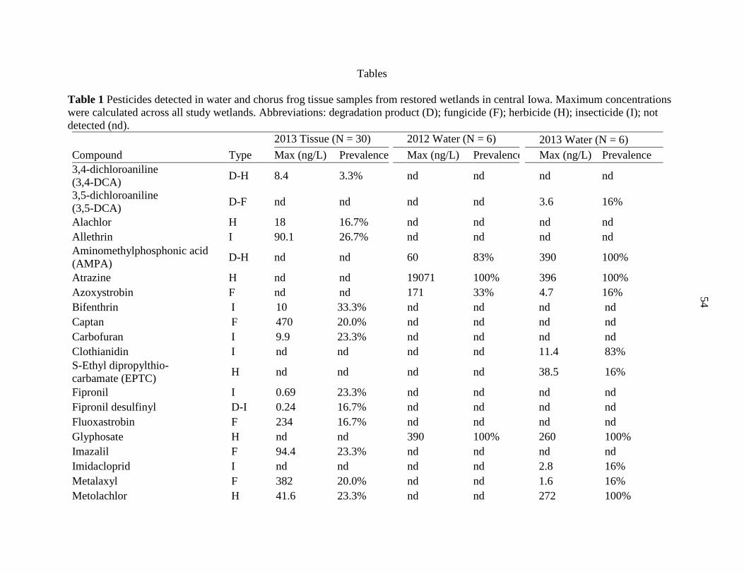
54

Tables

Table 1 Pesticides detected in water and chorus frog tissue samples from restored wetlands in central Iowa. Maximum concentrations

were calculated across all study wetlands. Abbreviations: degradation product (D); fungicide (F); herbicide (H); insecticide (I); not

detected (nd).

2013 Tissue (N = 30) 2012 Water (N = 6) 2013 Water (N = 6)

Compound Type Max (ng/L) Prevalence Max (ng/L) Prevalence Max (ng/L) Prevalence

3,4-dichloroaniline

(3,4-DCA) D-H 8.4 3.3% nd nd nd nd

3,5-dichloroaniline

(3,5-DCA) D-F nd nd nd nd 3.6 16%

Alachlor H 18 16.7% nd nd nd nd

Allethrin I 90.1 26.7% nd nd nd nd

Aminomethylphosphonic acid

(AMPA) D-H nd nd 60 83% 390 100%

Atrazine H nd nd 19071 100% 396 100%

Azoxystrobin F nd nd 171 33% 4.7 16%

Bifenthrin I 10 33.3% nd nd nd nd

Captan F 470 20.0% nd nd nd nd

Carbofuran I 9.9 23.3% nd nd nd nd

Clothianidin I nd nd nd nd 11.4 83%

S-Ethyl dipropylthio-

carbamate (EPTC) H nd nd nd nd 38.5 16%

Fipronil I 0.69 23.3% nd nd nd nd

Fipronil desulfinyl D-I 0.24 16.7% nd nd nd nd

Fluoxastrobin F 234 16.7% nd nd nd nd

Glyphosate H nd nd 390 100% 260 100%

Imazalil F 94.4 23.3% nd nd nd nd

Imidacloprid I nd nd nd nd 2.8 16%

Metalaxyl F 382 20.0% nd nd 1.6 16%

Metolachlor H 41.6 23.3% nd nd 272 100%

54

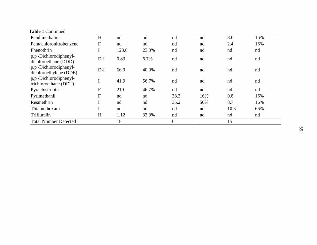
55

Table 1 Continued

Pendimethalin H nd nd nd nd 8.6 16%

Pentachloronitrobenzene F nd nd nd nd 2.4 16%

Phenothrin I 123.6 23.3% nd nd nd nd

p,p'-Dichlorodiphenyl-

dichloroethane (DDD) D-I 0.83 6.7% nd nd nd nd

p,p'-Dichlorodiphenyl-

dichloroethylene (DDE) D-I 66.9 40.0% nd nd nd nd

p,p'-Dichlorodiphenyl-

trichloroethane (DDT) I 41.9 56.7% nd nd nd nd

Pyraclostrobin F 210 46.7% nd nd nd nd

Pyrimethanil F nd nd 38.3 16% 0.8 16%

Resmethrin I nd nd 35.2 50% 8.7 16%

Thiamethoxam I nd nd nd nd 10.3 66%

Trifluralin H 1.12 33.3% nd nd nd nd

Total Number Detected 18 6 15

55

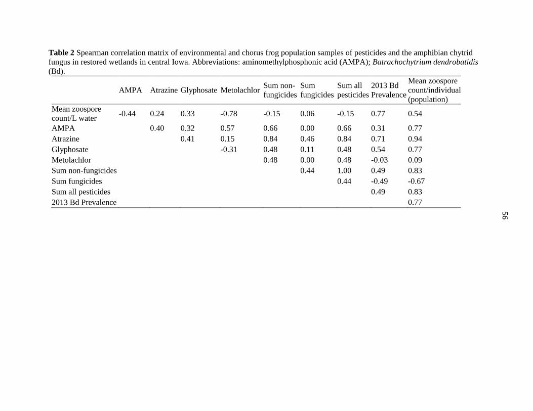
56

Table 2 Spearman correlation matrix of environmental and chorus frog population samples of pesticides and the amphibian chytrid

fungus in restored wetlands in central Iowa. Abbreviations: aminomethylphosphonic acid (AMPA); Batrachochytrium dendrobatidis

(Bd).

AMPA Atrazine Glyphosate Metolachlor

Sum non-

fungicides

Sum

fungicides

Sum all

pesticides

2013 Bd

Prevalence

Mean zoospore

count/individual

(population)

Mean zoospore

count/L water -0.44 0.24 0.33 -0.78 -0.15 0.06 -0.15 0.77 0.54

AMPA

0.40 0.32 0.57 0.66 0.00 0.66 0.31 0.77

Atrazine

0.41 0.15 0.84 0.46 0.84 0.71 0.94

Glyphosate

-0.31 0.48 0.11 0.48 0.54 0.77

Metolachlor

0.48 0.00 0.48 -0.03 0.09

Sum non-fungicides

0.44 1.00 0.49 0.83

Sum fungicides

0.44 -0.49 -0.67

Sum all pesticides

0.49 0.83

2013 Bd Prevalence

0.77

56

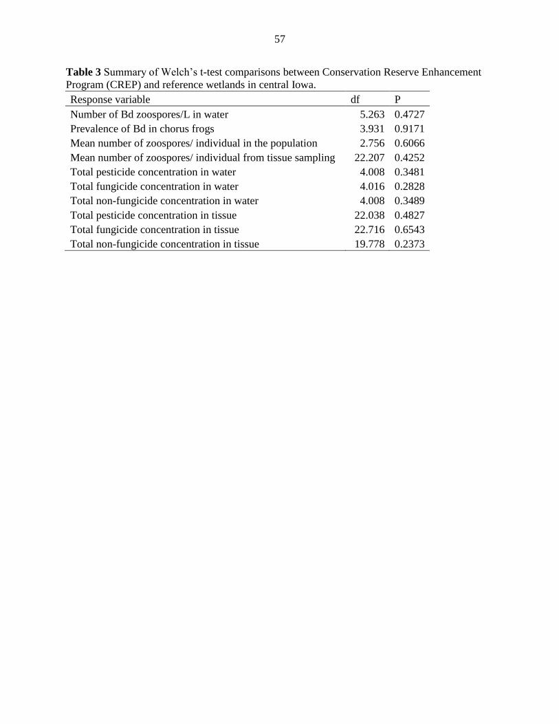
57

Table 3 Summary of Welch’s t-test comparisons between Conservation Reserve Enhancement

Program (CREP) and reference wetlands in central Iowa.

Response variable df P

Number of Bd zoospores/L in water 5.263 0.4727

Prevalence of Bd in chorus frogs 3.931 0.9171

Mean number of zoospores/ individual in the population 2.756 0.6066

Mean number of zoospores/ individual from tissue sampling 22.207 0.4252

Total pesticide concentration in water 4.008 0.3481

Total fungicide concentration in water 4.016 0.2828

Total non-fungicide concentration in water 4.008 0.3489

Total pesticide concentration in tissue 22.038 0.4827

Total fungicide concentration in tissue 22.716 0.6543

Total non-fungicide concentration in tissue 19.778 0.2373

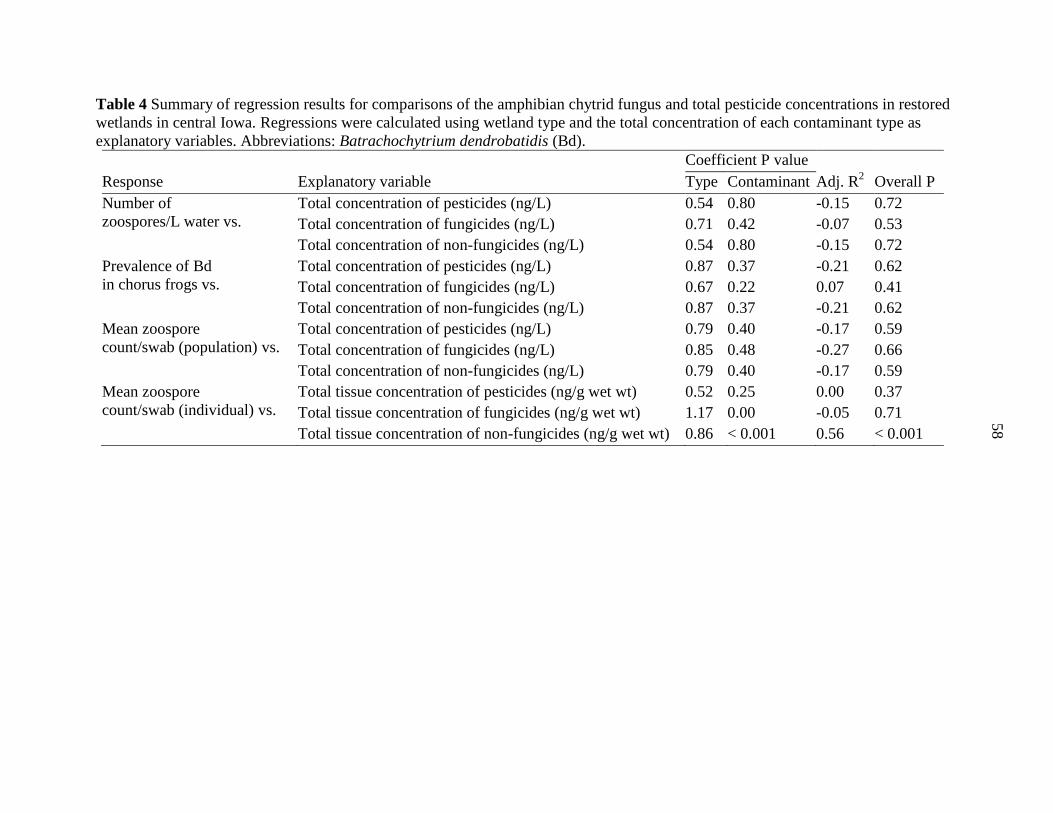
58

Table 4 Summary of regression results for comparisons of the amphibian chytrid fungus and total pesticide concentrations in restored

wetlands in central Iowa. Regressions were calculated using wetland type and the total concentration of each contaminant type as

explanatory variables. Abbreviations: Batrachochytrium dendrobatidis (Bd).

Coefficient P value

Response Explanatory variable Type Contaminant Adj. R2 Overall P

Number of

zoospores/L water vs.

Total concentration of pesticides (ng/L) 0.54 0.80 -0.15 0.72

Total concentration of fungicides (ng/L) 0.71 0.42 -0.07 0.53

Total concentration of non-fungicides (ng/L) 0.54 0.80 -0.15 0.72

Prevalence of Bd

in chorus frogs vs.

Total concentration of pesticides (ng/L) 0.87 0.37 -0.21 0.62

Total concentration of fungicides (ng/L) 0.67 0.22 0.07 0.41

Total concentration of non-fungicides (ng/L) 0.87 0.37 -0.21 0.62

Mean zoospore

count/swab (population) vs.

Total concentration of pesticides (ng/L) 0.79 0.40 -0.17 0.59

Total concentration of fungicides (ng/L) 0.85 0.48 -0.27 0.66

Total concentration of non-fungicides (ng/L) 0.79 0.40 -0.17 0.59

Mean zoospore

count/swab (individual) vs.

Total tissue concentration of pesticides (ng/g wet wt) 0.52 0.25 0.00 0.37

Total tissue concentration of fungicides (ng/g wet wt) 1.17 0.00 -0.05 0.71

Total tissue concentration of non-fungicides (ng/g wet wt) 0.86 < 0.001 0.56 < 0.001

58

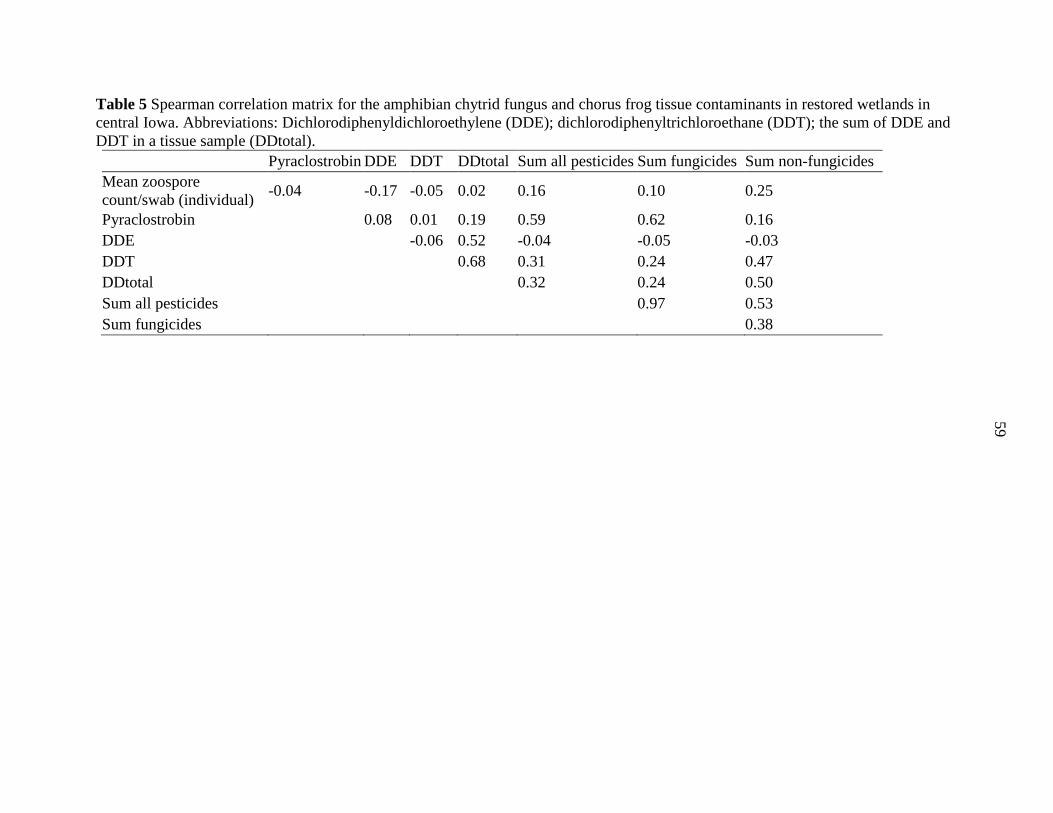
59

Table 5 Spearman correlation matrix for the amphibian chytrid fungus and chorus frog tissue contaminants in restored wetlands in

central Iowa. Abbreviations: Dichlorodiphenyldichloroethylene (DDE); dichlorodiphenyltrichloroethane (DDT); the sum of DDE and

DDT in a tissue sample (DDtotal).

Pyraclostrobin DDE DDT DDtotal Sum all pesticides Sum fungicides Sum non-fungicides

Mean zoospore

count/swab (individual) -0.04 -0.17 -0.05 0.02 0.16 0.10 0.25

Pyraclostrobin

0.08 0.01 0.19 0.59 0.62 0.16

DDE

-0.06 0.52 -0.04 -0.05 -0.03

DDT

0.68 0.31 0.24 0.47

DDtotal

0.32 0.24 0.50

Sum all pesticides

0.97 0.53

Sum fungicides

0.38

59

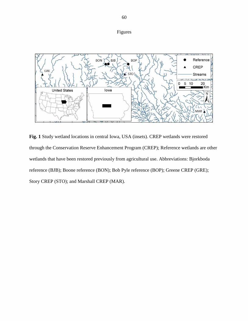
60

Figures

Fig. 1 Study wetland locations in central Iowa, USA (insets). CREP wetlands were restored

through the Conservation Reserve Enhancement Program (CREP); Reference wetlands are other

wetlands that have been restored previously from agricultural use. Abbreviations: Bjorkboda

reference (BJB); Boone reference (BON); Bob Pyle reference (BOP); Greene CREP (GRE);

Story CREP (STO); and Marshall CREP (MAR).

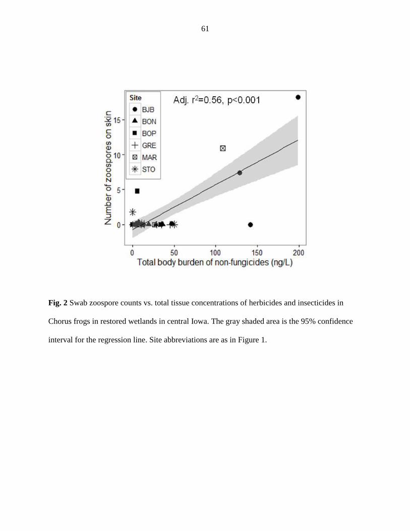
61

Fig. 2 Swab zoospore counts vs. total tissue concentrations of herbicides and insecticides in

Chorus frogs in restored wetlands in central Iowa. The gray shaded area is the 95% confidence

interval for the regression line. Site abbreviations are as in Figure 1.

62

CHAPTER 4. CONCLUSIONS

Summary

In this study, CREP and reference wetlands offered different qualities of

amphibian habitat and variations in environmental stressors at different wetlands related

differently to lethal and sub-lethal amphibian responses. While there were few differences in

amphibian species richness and no difference in estimated monthly survival probabilities

between wetland types, there were differences in developmental stress levels in frogs from

different wetlands. There was also variation in the way that environmental stressors interacted

with one another.

CREP wetlands were characterized by higher nitrogen concentrations, more alkaline pH,

slightly longer hydroperiods, and greater depths. Differences in structural characteristics may

have contributed to the increased prevalence of non-native bullfrogs and fish, while high

nitrogen concentrations may increase the risk of trematode parasitism for resident amphibians.

High pH and high nitrogen availability can lead to higher concentrations of ammonia which can

cause reduced survival, higher rates of deformity, and decreased growth and development in

tadpoles (Jofre & Karasov, 1999). While we did not detect differences in adult leopard frog

survival probabilities between the two wetland types, the lack of leopard frogs at Marshall CREP

is likely related to the presence of several species of predatory fish (Porej & Hetherington, 2005;

Walston & Mullin, 2007).

Unfortunately, these physical characteristics are central to the primary nitrogen removal

functions of CREP wetlands, so cannot be easily avoided. Mechanical draw downs, which are

already recommended on an as-needed basis for emergent vegetation management in CREP

wetlands, could have an added benefit of reducing the impact of predators such as bullfrogs and

63

fish on native amphibian species (Rowe & Garcia, 2014). The availability of wetlands with a

variety of hydroperiods is likely to be beneficial to the persistence of amphibian populations in

such an altered landscape, with deep wetlands providing overwintering sites for leopard frogs

and refuge during drought, and shallower wetlands providing refuge from predators (McCaffery

et al., 2014). Wetland variability may become increasingly important given the increasing

variability in rainfall forecasted for the Midwest due to climate change (Wuebbles & Hayhoe,

2004).

This study also highlighted the importance of other conservation practices in the

Midwest. The return rate of temporarily emigrated leopard frogs was relatively low in this study

(13%) which indicates that individuals are leaving the wetland after the breeding period and are

not likely to return within the next month. Individuals leaving wetlands likely travel into

surrounding upland areas, so having perennial upland buffers surrounding wetlands is likely very

important. Conservation practices such as grassed waterways and strips of perennial vegetation

within fields may contribute to an amphibian’s ability to move from wetland to wetland and may

be integral for influencing the colonization of new wetlands. Further study on where leopard

frogs go when they leave wetlands after breeding could be very useful in planning for the long

term persistence of the species.

There were a wide variety of potential environmental stressors experienced by frogs in

this study. While studies have begun to examine the ways in which these stressors interact, much

still remains to be learned. In this study, the concentrations of fungicides and non-fungicides

interacted differently with the abundance and prevalence of the amphibian chytrid fungus. While

the concentration of Bd zoospores in water samples did not appear to be related to the total

concentrations of fungicides and non-fungicides in water samples, the abundance of zoospores

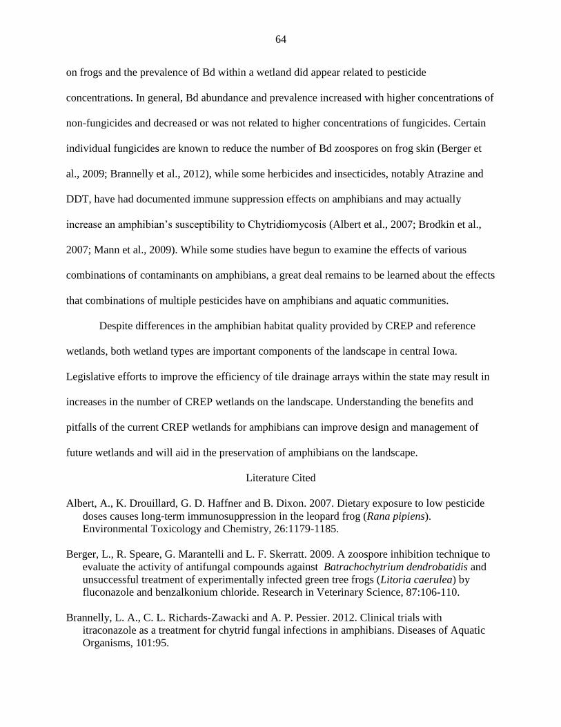
64

on frogs and the prevalence of Bd within a wetland did appear related to pesticide

concentrations. In general, Bd abundance and prevalence increased with higher concentrations of

non-fungicides and decreased or was not related to higher concentrations of fungicides. Certain

individual fungicides are known to reduce the number of Bd zoospores on frog skin (Berger et

al., 2009; Brannelly et al., 2012), while some herbicides and insecticides, notably Atrazine and

DDT, have had documented immune suppression effects on amphibians and may actually

increase an amphibian’s susceptibility to Chytridiomycosis (Albert et al., 2007; Brodkin et al.,

2007; Mann et al., 2009). While some studies have begun to examine the effects of various

combinations of contaminants on amphibians, a great deal remains to be learned about the effects

that combinations of multiple pesticides have on amphibians and aquatic communities.

Despite differences in the amphibian habitat quality provided by CREP and reference

wetlands, both wetland types are important components of the landscape in central Iowa.

Legislative efforts to improve the efficiency of tile drainage arrays within the state may result in

increases in the number of CREP wetlands on the landscape. Understanding the benefits and

pitfalls of the current CREP wetlands for amphibians can improve design and management of

future wetlands and will aid in the preservation of amphibians on the landscape.

Literature Cited

Albert, A., K. Drouillard, G. D. Haffner and B. Dixon. 2007. Dietary exposure to low pesticide

doses causes long‐term immunosuppression in the leopard frog (Rana pipiens).

Environmental Toxicology and Chemistry, 26:1179-1185.

Berger, L., R. Speare, G. Marantelli and L. F. Skerratt. 2009. A zoospore inhibition technique to

evaluate the activity of antifungal compounds against Batrachochytrium dendrobatidis and

unsuccessful treatment of experimentally infected green tree frogs (Litoria caerulea) by

fluconazole and benzalkonium chloride. Research in Veterinary Science, 87:106-110.

Brannelly, L. A., C. L. Richards-Zawacki and A. P. Pessier. 2012. Clinical trials with

itraconazole as a treatment for chytrid fungal infections in amphibians. Diseases of Aquatic

Organisms, 101:95.

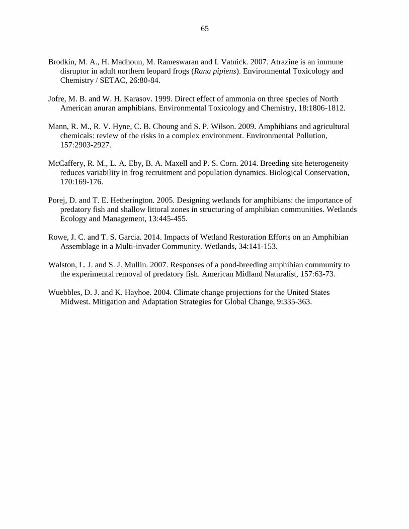
65

Brodkin, M. A., H. Madhoun, M. Rameswaran and I. Vatnick. 2007. Atrazine is an immune

disruptor in adult northern leopard frogs (Rana pipiens). Environmental Toxicology and

Chemistry / SETAC, 26:80-84.

Jofre, M. B. and W. H. Karasov. 1999. Direct effect of ammonia on three species of North

American anuran amphibians. Environmental Toxicology and Chemistry, 18:1806-1812.

Mann, R. M., R. V. Hyne, C. B. Choung and S. P. Wilson. 2009. Amphibians and agricultural

chemicals: review of the risks in a complex environment. Environmental Pollution,

157:2903-2927.

McCaffery, R. M., L. A. Eby, B. A. Maxell and P. S. Corn. 2014. Breeding site heterogeneity

reduces variability in frog recruitment and population dynamics. Biological Conservation,

170:169-176.

Porej, D. and T. E. Hetherington. 2005. Designing wetlands for amphibians: the importance of

predatory fish and shallow littoral zones in structuring of amphibian communities. Wetlands

Ecology and Management, 13:445-455.

Rowe, J. C. and T. S. Garcia. 2014. Impacts of Wetland Restoration Efforts on an Amphibian

Assemblage in a Multi-invader Community. Wetlands, 34:141-153.

Walston, L. J. and S. J. Mullin. 2007. Responses of a pond-breeding amphibian community to

the experimental removal of predatory fish. American Midland Naturalist, 157:63-73.

Wuebbles, D. J. and K. Hayhoe. 2004. Climate change projections for the United States

Midwest. Mitigation and Adaptation Strategies for Global Change, 9:335-363.

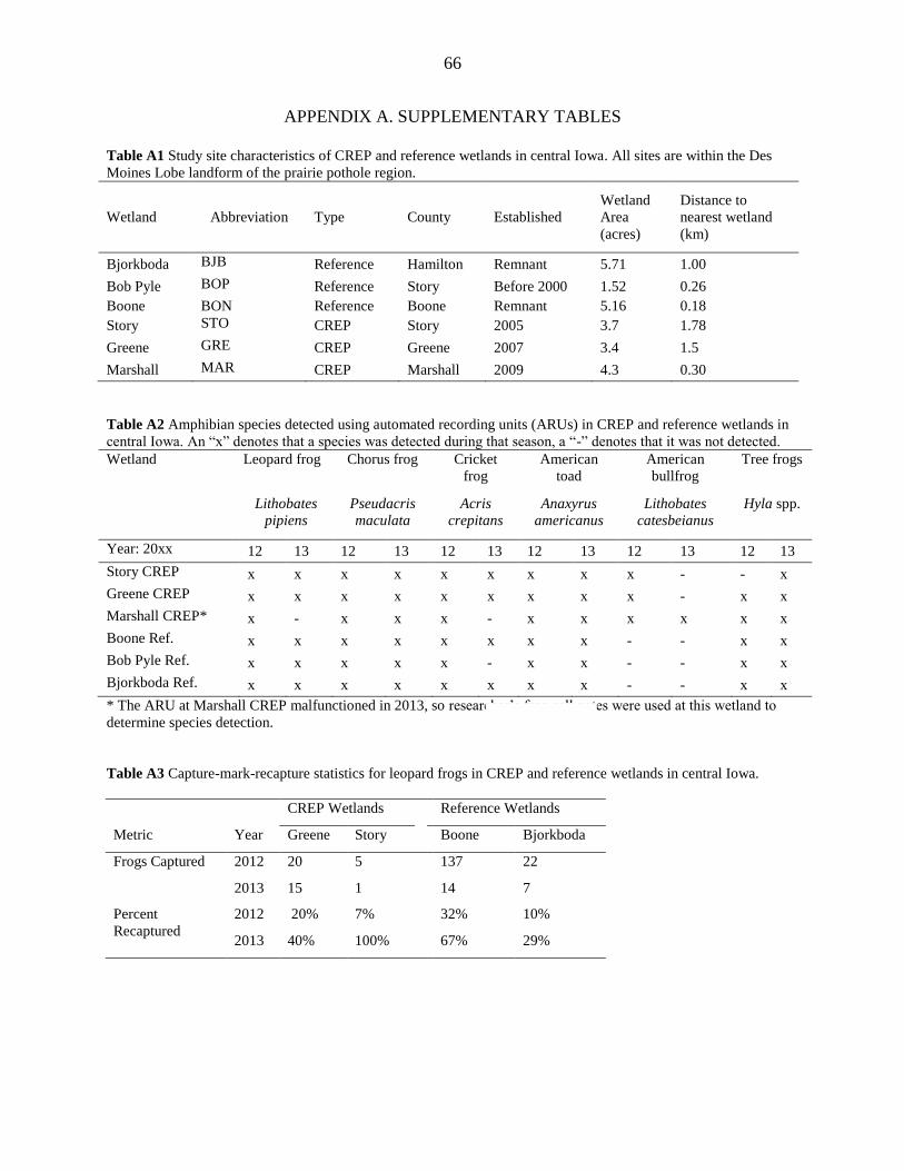
66

APPENDIX A. SUPPLEMENTARY TABLES

Table A1 Study site characteristics of CREP and reference wetlands in central Iowa. All sites are within the Des

Moines Lobe landform of the prairie pothole region.

Wetland Abbreviation Type County Established

Wetland

Area

(acres)

Distance to

nearest wetland

(km)

Bjorkboda BJB Reference Hamilton Remnant 5.71 1.00

Bob Pyle BOP Reference Story Before 2000 1.52 0.26

Boone BON Reference Boone Remnant 5.16 0.18

Story STO CREP Story 2005 3.7 1.78

Greene GRE CREP Greene 2007 3.4 1.5

Marshall MAR CREP Marshall 2009 4.3 0.30

Table A2 Amphibian species detected using automated recording units (ARUs) in CREP and reference wetlands in

central Iowa. An “x” denotes that a species was detected during that season, a “-” denotes that it was not detected.

Wetland Leopard frog Chorus frog Cricket

frog

American

toad

American

bullfrog

Tree frogs

Lithobates

pipiens

Pseudacris

maculata

Acris

crepitans

Anaxyrus

americanus

Lithobates

catesbeianus

Hyla spp.

Year: 20xx 12 13 12 13 12 13 12 13 12 13 12 13

Story CREP x x x x x x x x x - - x

Greene CREP x x x x x x x x x - x x

Marshall CREP* x - x x x - x x x x x x

Boone Ref. x x x x x x x x - - x x

Bob Pyle Ref. x x x x x - x x - - x x

Bjorkboda Ref. x x x x x x x x - - x x

* The ARU at Marshall CREP malfunctioned in 2013, so researcher’s frog call notes were used at this wetland to

determine species detection.

Table A3 Capture-mark-recapture statistics for leopard frogs in CREP and reference wetlands in central Iowa.

CREP Wetlands Reference Wetlands

Metric Year Greene Story Boone Bjorkboda

Frogs Captured 2012 20 5 137 22

2013 15 1 14 7

Percent

Recaptured

2012 20% 7% 32% 10%

2013 40% 100% 67% 29%

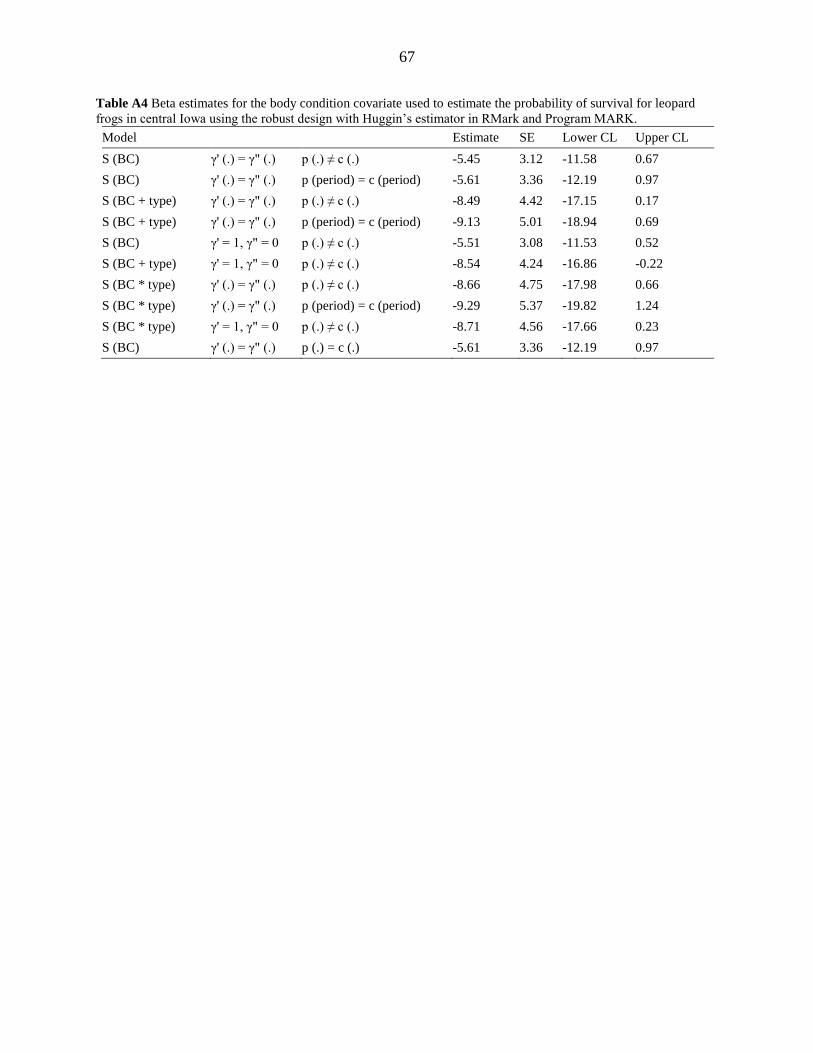
67

Table A4 Beta estimates for the body condition covariate used to estimate the probability of survival for leopard

frogs in central Iowa using the robust design with Huggin’s estimator in RMark and Program MARK.

Model

Estimate SE Lower CL Upper CL

S (BC) γ' (.) = γ" (.) p (.) ≠ c (.) -5.45 3.12 -11.58 0.67

S (BC) γ' (.) = γ" (.) p (period) = c (period) -5.61 3.36 -12.19 0.97

S (BC + type) γ' (.) = γ" (.) p (.) ≠ c (.) -8.49 4.42 -17.15 0.17

S (BC + type) γ' (.) = γ" (.) p (period) = c (period) -9.13 5.01 -18.94 0.69

S (BC) γ' = 1, γ" = 0 p (.) ≠ c (.) -5.51 3.08 -11.53 0.52

S (BC + type) γ' = 1, γ" = 0 p (.) ≠ c (.) -8.54 4.24 -16.86 -0.22

S (BC * type) γ' (.) = γ" (.) p (.) ≠ c (.) -8.66 4.75 -17.98 0.66

S (BC * type) γ' (.) = γ" (.) p (period) = c (period) -9.29 5.37 -19.82 1.24

S (BC * type) γ' = 1, γ" = 0 p (.) ≠ c (.) -8.71 4.56 -17.66 0.23

S (BC) γ' (.) = γ" (.) p (.) = c (.) -5.61 3.36 -12.19 0.97

68

APPENDIX B. EXPANDED METHODS

Environmental Characteristics We assessed water samples for phosphorous and nitrogen concentrations, pH, conductivity, and turbidity

three times throughout the growing season (April or May, June, and July) in 2012 and 2013. Samples were collected

in pre-sterilized bottles from the outflow point of the wetland and shipped to the United States Geological Survey

(USGS) National Water Quality Laboratory (NWQL), in Denver, CO, the same day. We collected two samples (125

ml each) for nutrient analysis and one for turbidity analysis (500 ml). One unfiltered nutrient sample was field

acidified using 1 ml of 4.5 M sulfuric acid, while the other was filtered using a 60 ml syringe and disk filter (USGS

Q460FLD). Total nitrogen and total phosphorous were analyzed in filtered and unfiltered water samples using

approved methods outlined in Patton and Kryskalla (2003). MDLs for total nitrogen, total phosphorous were 0.05

and 0.003 mg/L, respectively. Conductivity (specific conductance, µS/cm@25°C) and pH were measured using a

calibrated YSI probe (model 556, YSI, Yellow Springs, Ohio, USA) at three points around the outflow of the

wetland. Turbidity was measured in unfiltered water using EPA Method 180.1 (USEPA, 1993). Readings were made

in a nephelometer and compared to reference suspensions, and a primary standard suspension was used to calibrate

the instrument. A secondary standard suspension was used as a daily calibration check and was monitored

periodically for deterioration using one of the primary standards (USEPA, 1993). The detection limit for turbidity

was 2 Nephelometric turbidity units (NTUs).

We estimated the mean and maximum observed depths for each wetland by systematically measuring depth

at ten points along each of five equally spaced transects. Transects ran along the shorter axis of the wetland, or

perpendicular to any flow. Any wetland drying that occurred during population estimation or water quality sampling

in 2012 was recorded, and the month of final drying was estimated.

Water samples (N = 3 per wetland, per year) were filtered in June 2012 and 2013 to assess the presence Bd.

We filtered water collected near the outflow of each wetland through three Sterivex 0.2 µM capsule filters (Fisher

Scientific # SVGP L10 RC), then injected each filter with 50 ml phosphate buffered saline (Sigma-Aldrich #P5368)

followed by air. We plugged the downstream ends of the filters using capillary sealant (Fisher Scientific #23-550-

112) and filled them with 0.9 mL cell lysis solution (Fisher Scientific #FP2301320) before sealing them with sterile

filter caps (Cole-Parmer # EW-45503-56). We immediately placed the filters on ice and shipped them to the USGS

NWQL for analysis. DNA was extracted from capsule filters by using a Puregene kit for tissue (Gentra Systems,

Valencia, Calif.) and amplified and analyzed by quantitative polymerase chain reaction (qPCR) technique following

methods established by Kirshtein and others (2007). Capsule filters were incubated at 55°C for 60 min under

continual rotation to extract DNA. The lysis mixture was removed from the capsule filter and stored at –20°C prior

to analysis. Purified DNA was analyzed by using qPCR on a MX4000 QPCR system (Statagene®, La Jolla, Calif.)

that used a Taq polymerase assay with a TaqMan MGB probe and cycling parameters as follows: one 9-minute step

at 95°C, then 50 cycles at 94°C for 30 seconds, and finally 60°C for 1 minute. A standard curve was constructed

from a dilution series of Bd zoospore extracts of a known concentration and data were expressed as zoospore

equivalents per liter.

Differences in water samples (Nitrogen, Phosphorus, pH, conductivity, and turbidity) were compared using

a multivariate analysis of variance (MANOVA) and subsequent individual two-way univariate analyses of variance

(ANOVAs) in the stats package in program R (R Core Team 2013, Vienna, Austria). Wetland type and sample year

were used as explanatory variables, while Nitrogen, Phosphorus, pH, conductivity, and turbidity were included as

response variables in the MANOVA. Reference wetlands dried before late season sampling in 2012, so late season

2012 reference wetland samples were not included in the analysis. A late season 2012 turbidity sample for Story

CREP was not available, so a value was imputed at the mean of the other two turbidity measurements (2 NTUs) for

that wetland, to allow use of the other data. Spearman correlations were calculated using the mean values of the

amphibian and environmental characteristics for each wetland. The number of Bd zoospores in water were also

compared using two-way a ANOVA with year and type as explanatory variables. Since depth was only measured in

2013, mean depth was compared using a one-way ANOVA with type as an explanatory variable.

Two fyke nets were placed in each wetland for one 24-hour period in 2012 and another in 2013 to

determine the presence of fish (Hubert et al. 2012). Each net had two 71 cm x 122 cm frames, 19 mm mesh, a 13 m

lead, and was equipped with two two-liter floats to prevent air-breathing species from drowning. Nets were set in 1-

2 m deep water, with the full extent of the lead stretched perpendicular to the shoreline. Captured fish were

identified to species and released alive.

69

Amphibian Characteristics An automated recording unit (ARU; Song Meter model SM1 and 2: Wildlife Acoustics Inc., Concord,

Massachusetts, USA) was placed in each wetland to assess the species present at the wetland determined by calling

during the breeding season (Waddle et al., 2009). ARUs were set to record for three minutes at the start of every

hour, from 1800 h until 0400 h each night, and from 1 April until 15 July. We identified species recorded using the

spectrogram viewer of Song Scope™ Bioacoustics Monitoring Software (Ver. 2.1A; Wildlife Acoustics Inc.,

Concord, Massachusetts, USA, Waddle et al., 2009). The spectrogram viewer rendered visual representations of the

audio files, and each potential frog call was sorted and verified audibly by a technician. The ARU in Marshall CREP

malfunctioned during 2013, so researcher’s notes on species heard while working in the wetland were substituted. In

addition to monitoring presence of native frog species we were also interested in the determining presence of

bullfrogs at each wetland, since bullfrogs are known to carry diseases, eat other frogs, and reduce the presence and

health of other amphibian species (Boone et al., 2004; Casper & Hendricks, 2005).

We sampled leopard frogs at four wetlands (two CREP and two reference) in 2012 and 2013 for population

size and survival analysis using a robust design framework (Pollock, 1982; Kendall & Nichols, 1995). During each

year, frogs were captured in two rounds of sampling (primary periods) which consisted of three capture occasions

within a ten day period. The first primary period began in May, and when all four wetlands had been sampled, the

next primary period was initiated approximately one month after the first. During each capture occasion, we

searched the wetland and the surrounding vegetation for leopard frogs for six person-hours. Frogs were captured by

hand and by net using single-use gloves and placed in plastic containers filled with 1-2 cm of water until they were

identified and measured. New captures were anesthetized using a dilute buffered solution of Tricaine

methanesulfonate (MS222, 0.5g/1 L water, Green, 2001) and were marked individually with disinfected (80% ethyl

alcohol) 12 mm passive integrated transponder (PIT) tags (Avid Identification Systems, Norco, CA). PIT tags were

placed in the dorsal lymph sac, along the spine, and wounds were sealed with VetBond Adhesive (Beaupre et al.,

2004; Ferner, 2007). We also recorded frog sex and age. Individuals with tails or signs of recently reabsorbed tails

were classified as metamorphs and not included in survival and population estimation.

Mass was determined for each individual to the nearest 1.0 g using a spring scale (Pesola Ag; Baar,

Switzerland), and the snout-to-urostyle length (SUL) was measured using digital calipers (Fowler Sylvac 150mm;

Model 54-100-444-0). We also measured the length of the radioulna, thumb, femur, tibiofibula, and foot on each

side of the body to the nearest 0.001mm (St-Amour et al., 2010). Each measurement was taken three times by one

investigator (RAR) with temporal separation to minimize bias (St-Amour et al., 2010). We released frogs back to

their wetlands when they were able to hop and swim normally (Green, 2001).

We used the residuals from a regression of log(mass) on log(snout-to-urostyle-length) to indicate body

condition for each frog (Băncilă et al., 2010). Positive residuals indicated that individuals were heavier than average

for their body length, which may indicate an increased abundance of food resources or less environmental stress

(Băncilă et al., 2010). We included adults as well as newly metamorphosed individuals that had already fully

absorbed their tail in the regression when we compared among wetlands, but only included adults when body

condition was incorporated into the population modeling.

We calculated fluctuating asymmetry as the absolute value of the difference between right and left limbs

(Gallant & Teather, 2001). For a limb to be acceptable for fluctuating asymmetry analysis, it ought to exhibit no

handedness or directional asymmetry (which indicates a genetic component to asymmetry, rather than

environmental stress), show no size dependence, and should be possible to measure accurately enough to detect

asymmetry (Gallant & Teather, 2001). We evaluated directional asymmetry using a two-sided t-test (µ=0). We

estimated measurement error among the three replicated measurements using a linear mixed-effect model fit by

restricted maximum likelihood from package lme4 (Bates et al., 2013) in program R (R Core Team 2013, Vienna,

Austria) since we had repeated measures. We included the individual as a random effect and limb length (e.g., right

foot, or left femur) as a response. We compared the standard deviation of the within-limb measurements to the mean

difference between right and left limbs to ensure that we measured limbs accurately enough to detect asymmetry.

We used another linear model to test for size dependant asymmetry. We included wetland, frog age, frog sex, and

mean SUL as independent variables and the log of the absolute value (+ 0.1) of the difference between median right

and left limbs as a response. Tibiofibula asymmetry was the limb that best met the necessary criteria for exploring

fluctuating asymmetry, so was the only limb included in further analyses. We compared tibiofibula fluctuating

asymmetry in CREP and reference wetlands using an ANOVA with wetland type, frog age, frog sex, and sample

year as explanatory variables and the absolute value of the differences between right and left limbs as the response.

In 2012, 20 leopard frogs (N = 5 from four wetlands) were sent to the USGS National Wildlife Health

Center in Madison, WI, USA to be necropsied and screened for Chytridiomycosis, parasite infection, and gross

malformations. Amphibians were examined under a dissecting microscope to look for any unusual lesions,

70

malformations, or other abnormalities. Any parasites detected were keyed out to genus, and species whenever

possible.

To prevent the possible transmission of pathogens between wetlands, we scrubbed off any soil and

disinfected equipment (e.g., waders and boots) in household bleach or allowed it to completely dry between

wetlands (Johnson et al., 2003). We also wore disposable gloves and changed them between handling individuals

(St-Amour et al., 2010).

We estimated demographic parameters for adults (e.g., population size and individual survival) using the

Robust Design with Huggin’s estimator models in package RMark (Laake, 2013) in R (R Core Team 2013, Vienna,

Austria) to build models for program MARK (White & Burnham, 1999). Analyses were performed using wetland as

a group variable, and individual covariates were included in the estimation of survival rate and the probabilities of

capture and recapture.

We included five models in the estimation of capture (p) and recapture (c) probabilities. We modeled a

constant probability of capture and recapture with no effect of trapping (no trap-happiness or trap-shyness) by

holding p and c constant and equal to one another (p(.) = c(.)). We modeled a constant probability of capture and

recapture with some effect of trapping by holding p and c constant but allowing them to vary independently (p (.) ≠

c (.)). Because our primary periods occurred in two different phases of the growing season, we allowed for changes

in vegetation height and water level by setting p and c equal to one another and allowing them to vary by primary

period (p (period) = c (period)). Because our wetlands were surrounded by vegetative buffers of varying

composition (e.g., old pasture, restored prairie, or reed canary grass) we allowed the probabilities of capture and

recapture to vary by wetland (p (wetland) = c (wetland)). We also allowed the probabilities of capture and recapture

to vary by wetland and period (p (wetland + period) = c (wetland + period)).

We included eight different models for survival (S) in the set. We allowed survival to remain constant (S

(.)), to vary over time (S (time)), to vary by wetland type (i.e., CREP or reference; S (type)), and to vary by wetland

(S (wetland)). We allowed survival to vary depending on an individual’s tibiofibula asymmetry (S(FA)) or body

condition (S(BC)). Because body condition was different in CREP and reference wetlands, we also included

combinations of body condition and wetland type as covariates to tease out sources of variation (S (BC * Type) and

S (BC + Type)).

The robust design with Huggin’s estimator model incorporates two parameters to estimate temporary

emigration, which helps decouple emigration from survival to give better estimates of the population dynamics

(Pollock, 1982; Kendall, 2014). The probability that an animal temporarily emigrates (or was previously within the

population under study but was outside the study area and will remain outside the study area through the next

interval) is given by γ’ (pronounced gamma prime, Kendall, 2014). The probability that an animal was present and

observable previously, but temporarily left at some point prior to the current interval, is given by γ” (pronounced

gamma double-prime, Kendall, 2014). The probability that an individual will return once it leaves is given by the

inverse of these parameters and is the return rate of temporary emigrants. Thus, the probability that an individual

that was previously outside the study area but has now returned is 1- γ’. We incorporated four possible movement

scenarios into our model. The first is the null, or no-temporary emigration, model. For the null model we fixed γ’ =

1 and γ” = 0. For the constant, random temporary emigration model, in which an individual’s current observability

does not depend on whether it was observable or unobservable previously, we made γ’ and γ” constant through time

and equal to one another (γ'(.) = γ"(.)). For the time-varying, random temporary emigration model, γ’ and γ” were

still equal to one another, but were allowed to vary through time (γ'(t) = γ"(t)). For the Markovian temporary

emigration model, γ’ and γ” were constant through time but not equal to one another (γ'(.) ≠ γ"(.)). We ran all

possible models and utilized the cumulative Akaike’s information criterion weights to determine the best models

(Doherty et al., 2012). We model averaged the estimates for all real and derived parameters (Doherty et al., 2012).

Literature Cited

Băncilă, R. I., R. Plăiaşu, M. Tudor, C. Samoilă and D. Cogălniceanu. 2012. Fluctuating Asymmetry in the Eurasian

Spur-Thighed Tortoise,Testudo graeca iberaLinneaus, 1758 (Testudines: Testudinidae). Chelonian

Conservation and Biology, 11:234-239.

Beaupre, S., E. Jacobson, H. Lillywhite and K. Zamudio. 2004. Guidelines for use of live amphibians and reptiles in

field and laboratory research. A publication of the American Society of Ichthyologists and Herpetologists,

approved by board of Governors.

Bates, D., M. Maechler and B. Bolker. 2013. lme4: Linear mixed-effects models using S4 classes, 2012. R package

version 0.999999-0.

71

Boone, M. D., E. E. Little and R. D. Semlitsch. 2004. Overwintered bullfrog tadpoles negatively affect salamanders

and anurans in native amphibian communities. Copeia, 2004:683-690.

Casper, G. S. and R. Hendricks. 2005. Rana catesbeiana. In M. Lannoo (ed.), Amphibian Declines. University of

California Press, Berkeley, CA USA.

Doherty, P. F., G. C. White and K. P. Burnham. 2012. Comparison of model building and selection strategies.

Journal of Ornithology, 152:317-323.

Ferner, J. 2007. A review of marking and individual recognition techniques for amphibian and reptiles.

Herpetological Circular 35. Society for the Study of Amphibians and Reptiles. Atlanta, GA, USA.

Gallant, N. and K. Teather. 2001. Differences in size, pigmentation, and fluctuating asymmetry in stressed and

nonstressed northern leopard frogs (Rana pipiens). Ecoscience, 8:430-436.

Green, D. E. 2001. Anesthesia of amphibians in the field. United States Geological Survey, Madison, WI, USA.

Hubert, W. A., K. L. Pope and J. M. Dettmers. 2012. Passive capture techniques. p. 223-265. In A. V. Zale, D. L.

Parrish and T. M. Sutton (eds.), Fisheries Techniques. American Fisheries Society, Bethesda, MD, USA.

Johnson, M. L., L. Berger, L. Philips and R. Speare. 2003. Fungicidal effects of chemical disinfectants, UV light,

desiccation and heat on the amphibian chytrid Batrachochytrium dendrobatidis. Diseases of Aquatic

Organisms, 57:255-260.

Kendall, W. 2014. The ‘robust design’. p. 15-01. In E. Cooch and G. C. White (eds.), Program MARK:‘A Gentle

Introduction.

Kendall, W. L. and J. D. Nichols. 1995. On the use of secondary capture-recapture samples to estimate temporary

emigration and breeding proportions. Journal of Applied Statistics, 22:751-762.

Kirshtein, J. D., C. W. Anderson, J. S. Wood, J. E. Longcore and M. A. Voytek. 2007. Quantitative PCR detection

of Batrachochytrium dendrobatidis DNA from sediments and water. Diseases of Aquatic Organisms, 77:11.

Laake, J. L. 2013. RMark: An R Interface for Analysis of Capture-Recapture Data with MARK. Alaska Fish

Science Center, National Oceanic and Atmosoheric Administration National Marine Fish Service, Seattle, WA,

USA.

Patton, C. J. and J. R. Kryskalla. 2003. Methods of analysis by the US Geological Survey National Water Quality

Laboratory: Evaluation of alkaline persulfate digestion as an alternative to kjeldahl digestion for determination

of total and dissolved nitrogen and phosphorus in water. US Department of the Interior, US Geological Survey.

Pollock, K. H. 1982. A capture-recapture design robust to unequal probability of capture. The Journal of Wildlife

Management:752-757.

St-Amour, V., T. W. J. Garner, A. I. Schulte-Hostedde and D. Lesbarreres. 2010. Effects of two amphibian

pathogens on the developmental stability of green frogs. Conservation Biology, 24:788-794.

USEPA. 1993. Method 180.1; Determination of turbidity by nephelometry. United States Environmental Protection

Agency.

Waddle, J. H., T. F. Thigpen and B. M. Glorioso. 2009. Efiicacy of automatic vocalization recognition software for

anuran monitoring. herpetological Conservation and Biology, 4:384-388.

White, G. C. and K. P. Burnham. 1999. Program MARK: survival estimation from populations of marked animals.

Bird Study, 46:120-139.

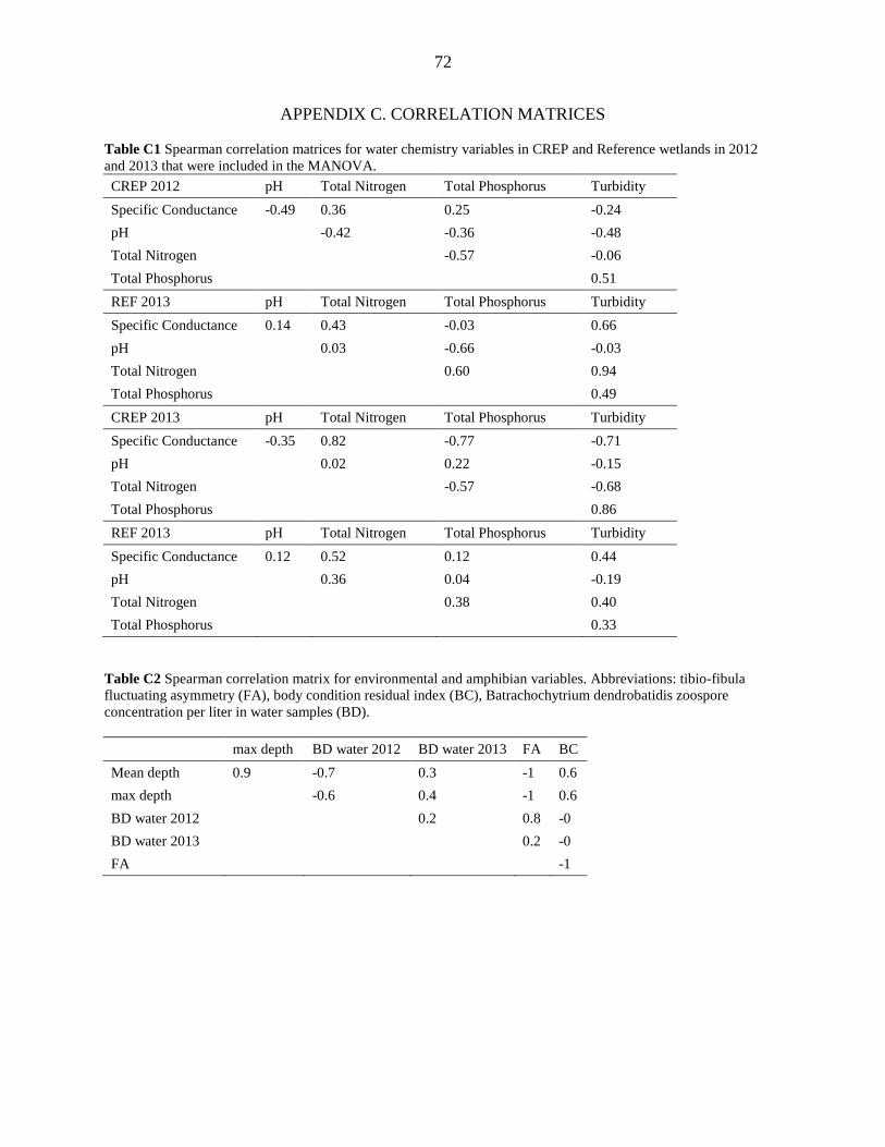
72

APPENDIX C. CORRELATION MATRICES

Table C1 Spearman correlation matrices for water chemistry variables in CREP and Reference wetlands in 2012

and 2013 that were included in the MANOVA.

CREP 2012 pH Total Nitrogen Total Phosphorus Turbidity

Specific Conductance -0.49 0.36 0.25 -0.24

pH

-0.42 -0.36 -0.48

Total Nitrogen

-0.57 -0.06

Total Phosphorus

0.51

REF 2013 pH Total Nitrogen Total Phosphorus Turbidity

Specific Conductance 0.14 0.43 -0.03 0.66

pH

0.03 -0.66 -0.03

Total Nitrogen

0.60 0.94

Total Phosphorus

0.49

CREP 2013 pH Total Nitrogen Total Phosphorus Turbidity

Specific Conductance -0.35 0.82 -0.77 -0.71

pH

0.02 0.22 -0.15

Total Nitrogen

-0.57 -0.68

Total Phosphorus

0.86

REF 2013 pH Total Nitrogen Total Phosphorus Turbidity

Specific Conductance 0.12 0.52 0.12 0.44

pH

0.36 0.04 -0.19

Total Nitrogen

0.38 0.40

Total Phosphorus

0.33

Table C2 Spearman correlation matrix for environmental and amphibian variables. Abbreviations: tibio-fibula

fluctuating asymmetry (FA), body condition residual index (BC), Batrachochytrium dendrobatidis zoospore

concentration per liter in water samples (BD).

max depth BD water 2012 BD water 2013 FA BC

Mean depth 0.9 -0.7 0.3 -1 0.6

max depth

-0.6 0.4 -1 0.6

BD water 2012

0.2 0.8 -0

BD water 2013

0.2 -0

FA

-1

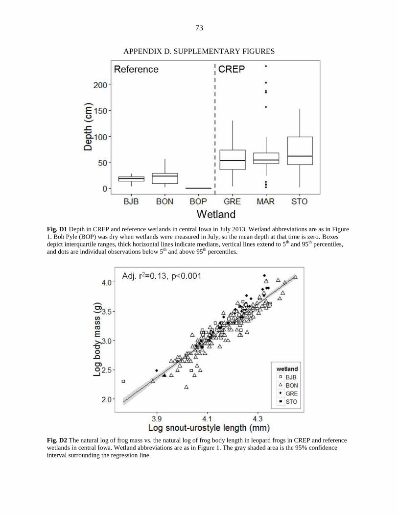
73

APPENDIX D. SUPPLEMENTARY FIGURES

Fig. D1 Depth in CREP and reference wetlands in central Iowa in July 2013. Wetland abbreviations are as in Figure

1. Bob Pyle (BOP) was dry when wetlands were measured in July, so the mean depth at that time is zero. Boxes

depict interquartile ranges, thick horizontal lines indicate medians, vertical lines extend to 5th

and 95th

percentiles,

and dots are individual observations below 5th

and above 95th percentiles.

Fig. D2 The natural log of frog mass vs. the natural log of frog body length in leopard frogs in CREP and reference

wetlands in central Iowa. Wetland abbreviations are as in Figure 1. The gray shaded area is the 95% confidence

interval surrounding the regression line.

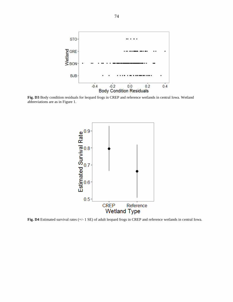
74

Fig. D3 Body condition residuals for leopard frogs in CREP and reference wetlands in central Iowa. Wetland

abbreviations are as in Figure 1.

Fig. D4 Estimated survival rates (+/- 1 SE) of adult leopard frogs in CREP and reference wetlands in central Iowa.

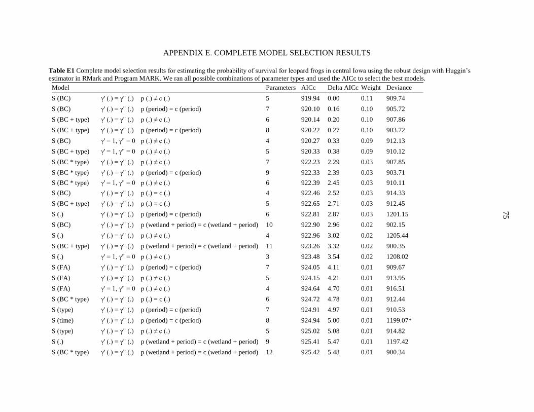
75

APPENDIX E. COMPLETE MODEL SELECTION RESULTS

Table E1 Complete model selection results for estimating the probability of survival for leopard frogs in central Iowa using the robust design with Huggin’s

estimator in RMark and Program MARK. We ran all possible combinations of parameter types and used the AICc to select the best models.

Model

Parameters AICc Delta AICc Weight Deviance

S (BC) γ' (.) = γ" (.) p (.) ≠ c (.) 5 919.94 0.00 0.11 909.74

S (BC) γ' (.) = γ" (.) p (period) = c (period) 7 920.10 0.16 0.10 905.72

S (BC + type) γ' (.) = γ" (.) p (.) ≠ c (.) 6 920.14 0.20 0.10 907.86

S (BC + type) γ' (.) = γ" (.) p (period) = c (period) 8 920.22 0.27 0.10 903.72

S (BC) γ' = 1, γ" = 0 p (.) ≠ c (.) 4 920.27 0.33 0.09 912.13

S (BC + type) γ' = 1, γ" = 0 p (.) ≠ c (.) 5 920.33 0.38 0.09 910.12

S (BC * type) γ' (.) = γ" (.) p (.) ≠ c (.) 7 922.23 2.29 0.03 907.85

S (BC * type) γ' (.) = γ" (.) p (period) = c (period) 9 922.33 2.39 0.03 903.71

S (BC * type) γ' = 1, γ" = 0 p (.) ≠ c (.) 6 922.39 2.45 0.03 910.11

S (BC) γ' (.) = γ" (.) p (.) = c (.) 4 922.46 2.52 0.03 914.33

S (BC + type) γ' (.) = γ" (.) p (.) = c (.) 5 922.65 2.71 0.03 912.45

S (.) γ' (.) = γ" (.) p (period) = c (period) 6 922.81 2.87 0.03 1201.15

S (BC) γ' (.) = γ" (.) p (wetland + period) = c (wetland + period) 10 922.90 2.96 0.02 902.15

S (.) γ' (.) = γ" (.) p (.) ≠ c (.) 4 922.96 3.02 0.02 1205.44

S (BC + type) γ' (.) = γ" (.) p (wetland + period) = c (wetland + period) 11 923.26 3.32 0.02 900.35

S (.) γ' = 1, γ" = 0 p (.) ≠ c (.) 3 923.48 3.54 0.02 1208.02

S (FA) γ' (.) = γ" (.) p (period) = c (period) 7 924.05 4.11 0.01 909.67

S (FA) γ' (.) = γ" (.) p (.) ≠ c (.) 5 924.15 4.21 0.01 913.95

S (FA) γ' = 1, γ" = 0 p (.) ≠ c (.) 4 924.64 4.70 0.01 916.51

S (BC * type) γ' (.) = γ" (.) p (.) = c (.) 6 924.72 4.78 0.01 912.44

S (type) γ' (.) = γ" (.) p (period) = c (period) 7 924.91 4.97 0.01 910.53

S (time) γ' (.) = γ" (.) p (period) = c (period) 8 924.94 5.00 0.01 1199.07*

S (type) γ' (.) = γ" (.) p (.) ≠ c (.) 5 925.02 5.08 0.01 914.82

S (.) γ' (.) = γ" (.) p (wetland + period) = c (wetland + period) 9 925.41 5.47 0.01 1197.42

S (BC * type) γ' (.) = γ" (.) p (wetland + period) = c (wetland + period) 12 925.42 5.48 0.01 900.34

75

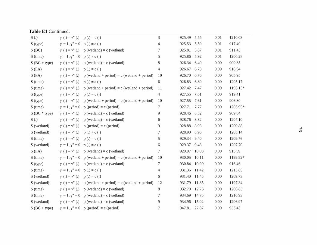
76

Table E1 Continued.

S (.) γ' (.) = γ" (.) p (.) = c (.) 3 925.49 5.55 0.01 1210.03

S (type) γ' = 1, γ" = 0 p (.) ≠ c (.) 4 925.53 5.59 0.01 917.40

S (BC) γ' (.) = γ" (.) p (wetland) = c (wetland) 7 925.81 5.87 0.01 911.43

S (time) γ' = 1, γ" = 0 p (.) ≠ c (.) 5 925.86 5.92 0.01 1206.28

S (BC + type) γ' (.) = γ" (.) p (wetland) = c (wetland) 8 926.34 6.40 0.00 909.85

S (FA) γ' (.) = γ" (.) p (.) = c (.) 4 926.67 6.73 0.00 918.54

S (FA) γ' (.) = γ" (.) p (wetland + period) = c (wetland + period) 10 926.70 6.76 0.00 905.95

S (time) γ' (.) = γ" (.) p (.) ≠ c (.) 6 926.83 6.89 0.00 1205.17

S (time) γ' (.) = γ" (.) p (wetland + period) = c (wetland + period) 11 927.42 7.47 0.00 1195.13*

S (type) γ' (.) = γ" (.) p (.) = c (.) 4 927.55 7.61 0.00 919.41

S (type) γ' (.) = γ" (.) p (wetland + period) = c (wetland + period) 10 927.55 7.61 0.00 906.80

S (time) γ' = 1, γ" = 0 p (period) = c (period) 7 927.71 7.77 0.00 1203.95*

S (BC * type) γ' (.) = γ" (.) p (wetland) = c (wetland) 9 928.46 8.52 0.00 909.84

S (.) γ' (.) = γ" (.) p (wetland) = c (wetland) 6 928.76 8.82 0.00 1207.10

S (wetland) γ' (.) = γ" (.) p (period) = c (period) 9 928.88 8.93 0.00 1200.88

S (wetland) γ' (.) = γ" (.) p (.) ≠ c (.) 7 928.90 8.96 0.00 1205.14

S (time) γ' (.) = γ" (.) p (.) = c (.) 5 929.34 9.40 0.00 1209.76

S (wetland) γ' = 1, γ" = 0 p (.) ≠ c (.) 6 929.37 9.43 0.00 1207.70

S (FA) γ' (.) = γ" (.) p (wetland) = c (wetland) 7 929.97 10.03 0.00 915.59

S (time) γ' = 1, γ" = 0 p (wetland + period) = c (wetland + period) 10 930.05 10.11 0.00 1199.92*

S (type) γ' (.) = γ" (.) p (wetland) = c (wetland) 7 930.84 10.90 0.00 916.46

S (time) γ' = 1, γ" = 0 p (.) = c (.) 4 931.36 11.42 0.00 1213.85

S (wetland) γ' (.) = γ" (.) p (.) = c (.) 6 931.40 11.45 0.00 1209.73

S (wetland) γ' (.) = γ" (.) p (wetland + period) = c (wetland + period) 12 931.79 11.85 0.00 1197.34

S (time) γ' (.) = γ" (.) p (wetland) = c (wetland) 8 932.70 12.76 0.00 1206.83

S (time) γ' = 1, γ" = 0 p (wetland) = c (wetland) 7 934.69 14.75 0.00 1210.93

S (wetland) γ' (.) = γ" (.) p (wetland) = c (wetland) 9 934.96 15.02 0.00 1206.97

S (BC + type) γ' = 1, γ" = 0 p (period) = c (period) 7 947.81 27.87 0.00 933.43

76

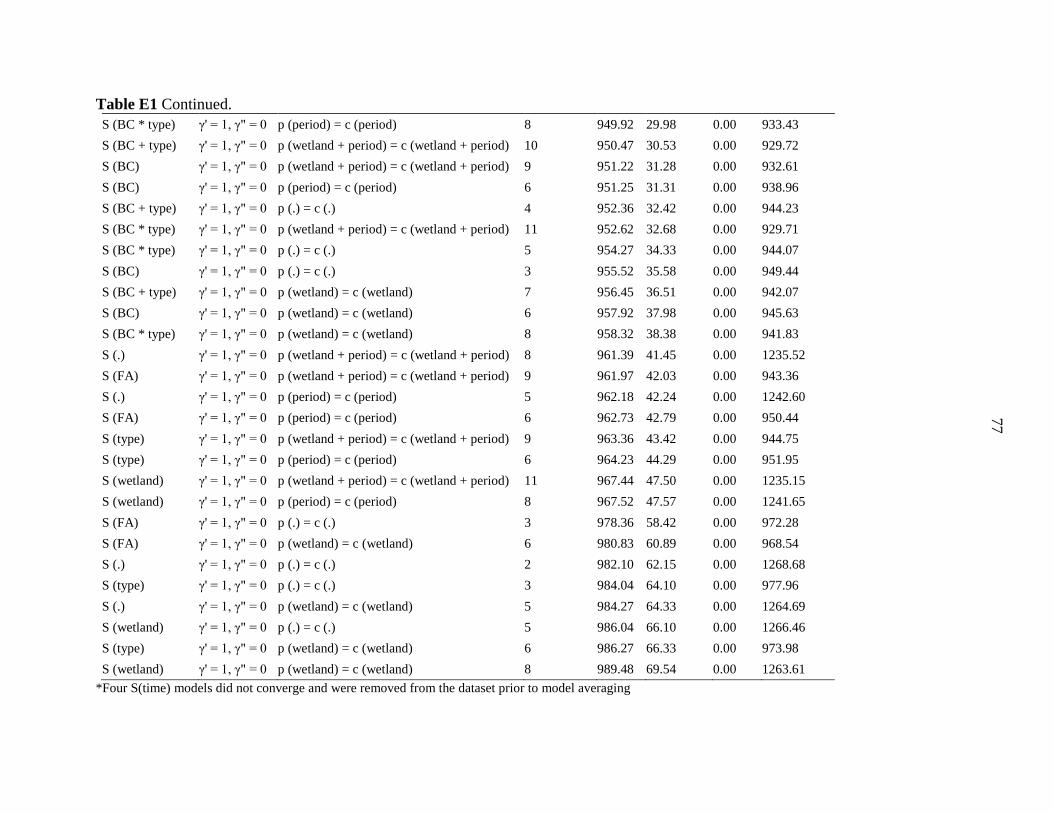
77

Table E1 Continued.

S (BC * type) γ' = 1, γ" = 0 p (period) = c (period) 8 949.92 29.98 0.00 933.43

S (BC + type) γ' = 1, γ" = 0 p (wetland + period) = c (wetland + period) 10 950.47 30.53 0.00 929.72

S (BC) γ' = 1, γ" = 0 p (wetland + period) = c (wetland + period) 9 951.22 31.28 0.00 932.61

S (BC) γ' = 1, γ" = 0 p (period) = c (period) 6 951.25 31.31 0.00 938.96

S (BC + type) γ' = 1, γ" = 0 p (.) = c (.) 4 952.36 32.42 0.00 944.23

S (BC * type) γ' = 1, γ" = 0 p (wetland + period) = c (wetland + period) 11 952.62 32.68 0.00 929.71

S (BC * type) γ' = 1, γ" = 0 p (.) = c (.) 5 954.27 34.33 0.00 944.07

S (BC) γ' = 1, γ" = 0 p (.) = c (.) 3 955.52 35.58 0.00 949.44

S (BC + type) γ' = 1, γ" = 0 p (wetland) = c (wetland) 7 956.45 36.51 0.00 942.07

S (BC) γ' = 1, γ" = 0 p (wetland) = c (wetland) 6 957.92 37.98 0.00 945.63

S (BC * type) γ' = 1, γ" = 0 p (wetland) = c (wetland) 8 958.32 38.38 0.00 941.83

S (.) γ' = 1, γ" = 0 p (wetland + period) = c (wetland + period) 8 961.39 41.45 0.00 1235.52

S (FA) γ' = 1, γ" = 0 p (wetland + period) = c (wetland + period) 9 961.97 42.03 0.00 943.36

S (.) γ' = 1, γ" = 0 p (period) = c (period) 5 962.18 42.24 0.00 1242.60

S (FA) γ' = 1, γ" = 0 p (period) = c (period) 6 962.73 42.79 0.00 950.44

S (type) γ' = 1, γ" = 0 p (wetland + period) = c (wetland + period) 9 963.36 43.42 0.00 944.75

S (type) γ' = 1, γ" = 0 p (period) = c (period) 6 964.23 44.29 0.00 951.95

S (wetland) γ' = 1, γ" = 0 p (wetland + period) = c (wetland + period) 11 967.44 47.50 0.00 1235.15

S (wetland) γ' = 1, γ" = 0 p (period) = c (period) 8 967.52 47.57 0.00 1241.65

S (FA) γ' = 1, γ" = 0 p (.) = c (.) 3 978.36 58.42 0.00 972.28

S (FA) γ' = 1, γ" = 0 p (wetland) = c (wetland) 6 980.83 60.89 0.00 968.54

S (.) γ' = 1, γ" = 0 p (.) = c (.) 2 982.10 62.15 0.00 1268.68

S (type) γ' = 1, γ" = 0 p (.) = c (.) 3 984.04 64.10 0.00 977.96

S (.) γ' = 1, γ" = 0 p (wetland) = c (wetland) 5 984.27 64.33 0.00 1264.69

S (wetland) γ' = 1, γ" = 0 p (.) = c (.) 5 986.04 66.10 0.00 1266.46

S (type) γ' = 1, γ" = 0 p (wetland) = c (wetland) 6 986.27 66.33 0.00 973.98

S (wetland) γ' = 1, γ" = 0 p (wetland) = c (wetland) 8 989.48 69.54 0.00 1263.61

*Four S(time) models did not converge and were removed from the dataset prior to model averaging

77

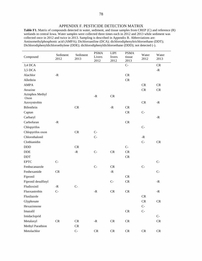
78

APPENDIX F. PESTICIDE DETECTION MATRIX

Table F1. Matrix of compounds detected in water, sediment, and tissue samples from CREP (C) and reference (R)

wetlands in central Iowa. Water samples were collected three times each in 2012 and 2013 while sediment was

collected once in 2012 and twice in 2013. Sampling is described in Appendix B. Abbreviations are:

Aminomethylphosphonic acid (AMPA); Dichloroaniline (DCA); dichlorodiphenyltrichloroethane (DDT);

Dichlorodiphenyldichloroethylene (DDE); dichlorodiphenyldichloroethane (DDD); not detected (-).

Compound Sediment

2012

Sediment

2013

PSMA

Livers

2012

LIPI

livers

2012

PSMA

tissue

2013

Water

2012

Water

2013

3,4 DCA

C-

CR

3,5 DCA

-R

Alachlor -R

CR

Allethrin

CR

AMPA

CR CR

Atrazine

CR CR

Azinphos Methyl

Oxon -R CR

Azoxystrobin

CR -R

Bifenthrin

CR

-R CR

Captan

CR C-

Carbaryl

-R

Carbofuran -R

CR

Chlopyrifos

C-

Chlopyrifos oxon

CR C-

Chlorothalonil

C-

-R

Clothianidin

C- CR

DDD

CR

C-

DDE

-R C- CR CR

DDT

CR

EPTC C-

C-

Fenbucanazole

C- CR

C-

Fenhexamide CR

-R

C-

Fipronil

CR

Fipronil desulfinyl

C- CR

-R

Fludioxinil -R C-

Fluoxastrobin C-

-R CR CR

-R

Flusilazole

CR

Glyphosate

CR CR

Hexazinnone

C-

Imazalil

CR C-

Imidacloprid

C-

Metalaxyl CR CR -R CR CR

CR

Methyl Parathion

CR

Metolachlor

C- CR CR CR CR CR

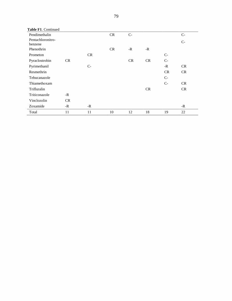
79

Table F1. Continued

Pendimethalin

CR C-

C-

Pentachloronitro-

benzene C-

Phenothrin

CR -R -R

Prometon

CR

C-

Pyraclostrobin CR

CR CR C-

Pyrimethanil

C-

-R CR

Resmethrin

CR CR

Tebucanazole

C-

Thiamethoxam

C- CR

Trifluralin

CR

CR

Triticonazole -R

Vinclozolin CR

Zoxamide -R -R

-R

Total 11 11 10 12 18 19 22

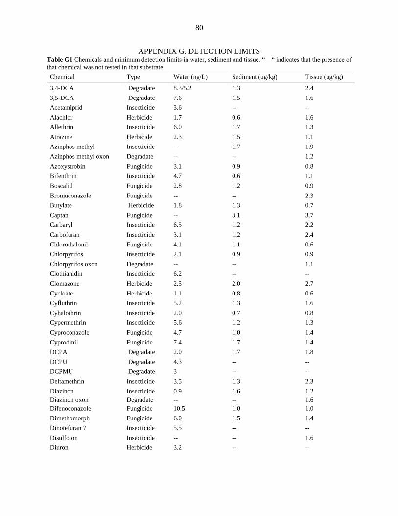
80

APPENDIX G. DETECTION LIMITS Table G1 Chemicals and minimum detection limits in water, sediment and tissue. “—“ indicates that the presence of

that chemical was not tested in that substrate.

Chemical Type Water (ng/L) Sediment (ug/kg) Tissue (ug/kg)

3,4-DCA Degradate 8.3/5.2 1.3 2.4

3,5-DCA Degradate 7.6 1.5 1.6

Acetamiprid Insecticide 3.6 -- --

Alachlor Herbicide 1.7 0.6 1.6

Allethrin Insecticide 6.0 1.7 1.3

Atrazine Herbicide 2.3 1.5 1.1

Azinphos methyl Insecticide -- 1.7 1.9

Azinphos methyl oxon Degradate -- -- 1.2

Azoxystrobin Fungicide 3.1 0.9 0.8

Bifenthrin Insecticide 4.7 0.6 1.1

Boscalid Fungicide 2.8 1.2 0.9

Bromuconazole Fungicide -- -- 2.3

Butylate Herbicide 1.8 1.3 0.7

Captan Fungicide -- 3.1 3.7

Carbaryl Insecticide 6.5 1.2 2.2

Carbofuran Insecticide 3.1 1.2 2.4

Chlorothalonil Fungicide 4.1 1.1 0.6

Chlorpyrifos Insecticide 2.1 0.9 0.9

Chlorpyrifos oxon Degradate -- -- 1.1

Clothianidin Insecticide 6.2 -- --

Clomazone Herbicide 2.5 2.0 2.7

Cycloate Herbicide 1.1 0.8 0.6

Cyfluthrin Insecticide 5.2 1.3 1.6

Cyhalothrin Insecticide 2.0 0.7 0.8

Cypermethrin Insecticide 5.6 1.2 1.3

Cyproconazole Fungicide 4.7 1.0 1.4

Cyprodinil Fungicide 7.4 1.7 1.4

DCPA Degradate 2.0 1.7 1.8

DCPU Degradate 4.3 -- --

DCPMU Degradate 3 -- --

Deltamethrin Insecticide 3.5 1.3 2.3

Diazinon Insecticide 0.9 1.6 1.2

Diazinon oxon Degradate -- -- 1.6

Difenoconazole Fungicide 10.5 1.0 1.0

Dimethomorph Fungicide 6.0 1.5 1.4

Dinotefuran ? Insecticide 5.5 -- --

Disulfoton Insecticide -- -- 1.6

Diuron Herbicide 3.2 -- --

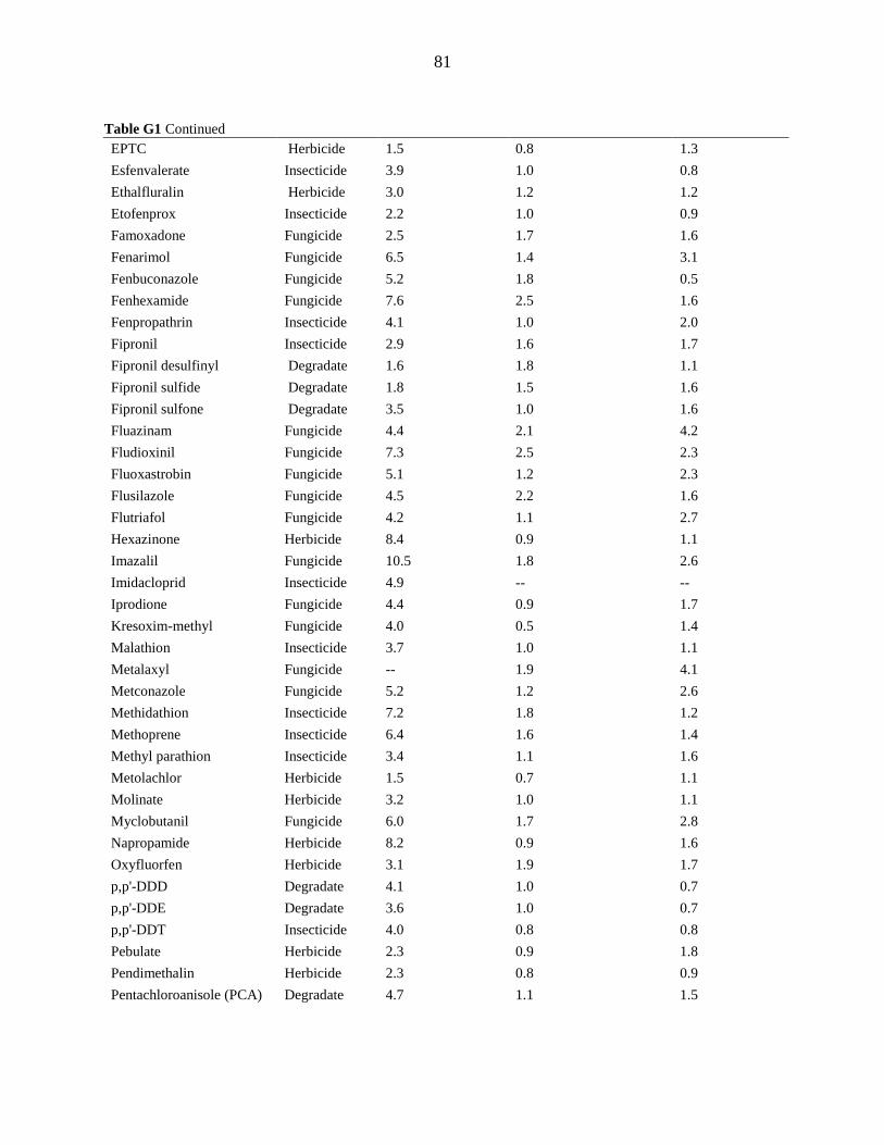
81

Table G1 Continued

EPTC Herbicide 1.5 0.8 1.3

Esfenvalerate Insecticide 3.9 1.0 0.8

Ethalfluralin Herbicide 3.0 1.2 1.2

Etofenprox Insecticide 2.2 1.0 0.9

Famoxadone Fungicide 2.5 1.7 1.6

Fenarimol Fungicide 6.5 1.4 3.1

Fenbuconazole Fungicide 5.2 1.8 0.5

Fenhexamide Fungicide 7.6 2.5 1.6

Fenpropathrin Insecticide 4.1 1.0 2.0

Fipronil Insecticide 2.9 1.6 1.7

Fipronil desulfinyl Degradate 1.6 1.8 1.1

Fipronil sulfide Degradate 1.8 1.5 1.6

Fipronil sulfone Degradate 3.5 1.0 1.6

Fluazinam Fungicide 4.4 2.1 4.2

Fludioxinil Fungicide 7.3 2.5 2.3

Fluoxastrobin Fungicide 5.1 1.2 2.3

Flusilazole Fungicide 4.5 2.2 1.6

Flutriafol Fungicide 4.2 1.1 2.7

Hexazinone Herbicide 8.4 0.9 1.1

Imazalil Fungicide 10.5 1.8 2.6

Imidacloprid Insecticide 4.9 -- --

Iprodione Fungicide 4.4 0.9 1.7

Kresoxim-methyl Fungicide 4.0 0.5 1.4

Malathion Insecticide 3.7 1.0 1.1

Metalaxyl Fungicide -- 1.9 4.1

Metconazole Fungicide 5.2 1.2 2.6

Methidathion Insecticide 7.2 1.8 1.2

Methoprene Insecticide 6.4 1.6 1.4

Methyl parathion Insecticide 3.4 1.1 1.6

Metolachlor Herbicide 1.5 0.7 1.1

Molinate Herbicide 3.2 1.0 1.1

Myclobutanil Fungicide 6.0 1.7 2.8

Napropamide Herbicide 8.2 0.9 1.6

Oxyfluorfen Herbicide 3.1 1.9 1.7

p,p'-DDD Degradate 4.1 1.0 0.7

p,p'-DDE Degradate 3.6 1.0 0.7

p,p'-DDT Insecticide 4.0 0.8 0.8

Pebulate Herbicide 2.3 0.9 1.8

Pendimethalin Herbicide 2.3 0.8 0.9

Pentachloroanisole (PCA) Degradate 4.7 1.1 1.5

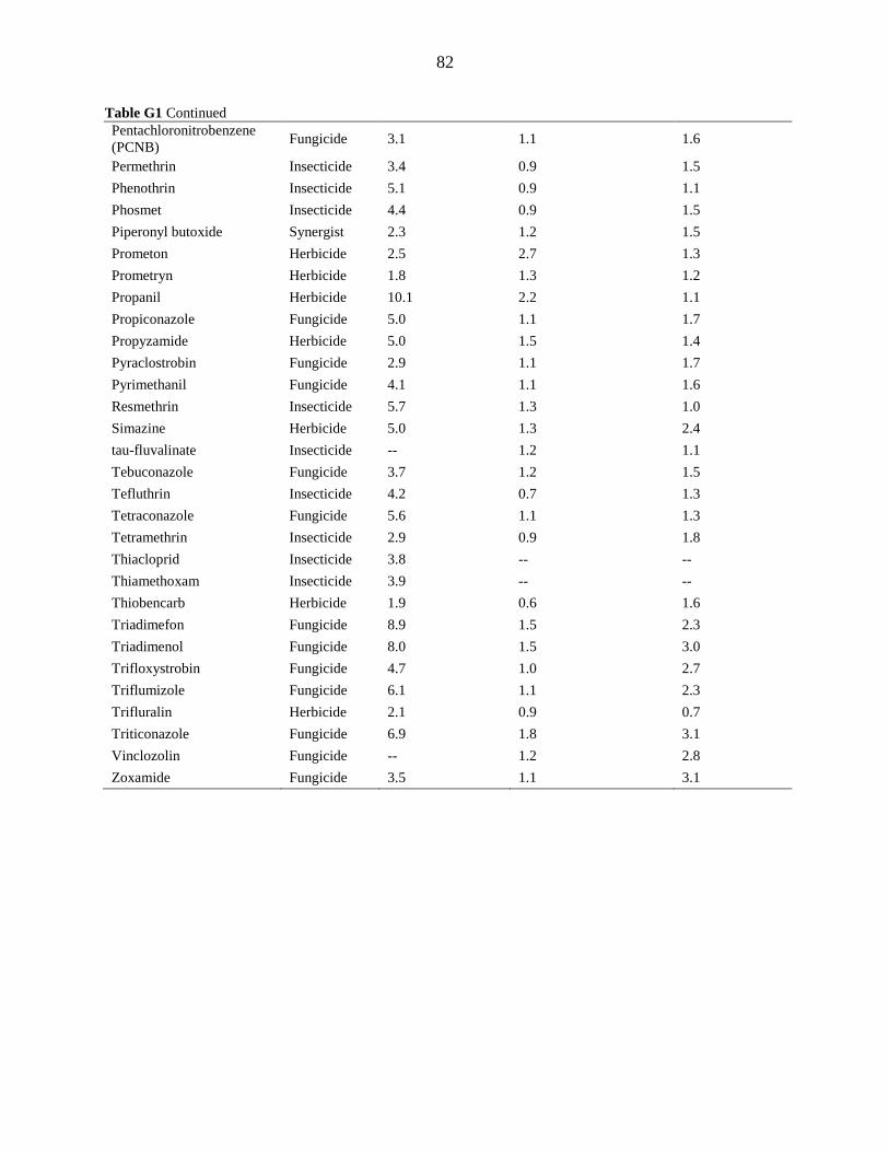
82

Table G1 Continued

Pentachloronitrobenzene

(PCNB) Fungicide 3.1 1.1 1.6

Permethrin Insecticide 3.4 0.9 1.5

Phenothrin Insecticide 5.1 0.9 1.1

Phosmet Insecticide 4.4 0.9 1.5

Piperonyl butoxide Synergist 2.3 1.2 1.5

Prometon Herbicide 2.5 2.7 1.3

Prometryn Herbicide 1.8 1.3 1.2

Propanil Herbicide 10.1 2.2 1.1

Propiconazole Fungicide 5.0 1.1 1.7

Propyzamide Herbicide 5.0 1.5 1.4

Pyraclostrobin Fungicide 2.9 1.1 1.7

Pyrimethanil Fungicide 4.1 1.1 1.6

Resmethrin Insecticide 5.7 1.3 1.0

Simazine Herbicide 5.0 1.3 2.4

tau-fluvalinate Insecticide -- 1.2 1.1

Tebuconazole Fungicide 3.7 1.2 1.5

Tefluthrin Insecticide 4.2 0.7 1.3

Tetraconazole Fungicide 5.6 1.1 1.3

Tetramethrin Insecticide 2.9 0.9 1.8

Thiacloprid Insecticide 3.8 -- --

Thiamethoxam Insecticide 3.9 -- --

Thiobencarb Herbicide 1.9 0.6 1.6

Triadimefon Fungicide 8.9 1.5 2.3

Triadimenol Fungicide 8.0 1.5 3.0

Trifloxystrobin Fungicide 4.7 1.0 2.7

Triflumizole Fungicide 6.1 1.1 2.3

Trifluralin Herbicide 2.1 0.9 0.7

Triticonazole Fungicide 6.9 1.8 3.1

Vinclozolin Fungicide -- 1.2 2.8

Zoxamide Fungicide 3.5 1.1 3.1

83

APPENDIX H. PARASITE ANALYSIS RESULTS In 2011 and 2012, leopard frogs, chorus frogs, and bullfrogs were sent to the US Geological Survey

National Wildlife Health Center in Madison, WI, USA to be necropsied and screened for Chytridiomycosis, parasite

infection, and gross malformations. Amphibians were examined under a dissecting microscope to look for any

unusual lesions, malformations, or other abnormalities. Any parasites detected were keyed out to genus, and species

whenever possible.

In 2011, a total of 34 individuals were sent from two wetlands. 10 chorus frogs, one bullfrog, and six

leopard frogs were sent from Bob Pyle reference, while nine chorus frogs and eight leopard frogs were sent from

Story CREP. The bullfrog and all of the leopard frogs had Chytridiomycosis (mild/moderate). Of the chorus frogs,

one individual from Story CREP and two individuals from Bob Pyle had Chytridiomycosis. A number of individuals

had parasite infections, including two individuals from Story CREP with nematodes in their gut, and two individuals

from Bob Pyle reference that had either nematode or cestode infections.

In 2012 there were several notable individuals. Ten chorus frogs (from two wetlands), 20 leopard frogs

(from four wetlands), and five bullfrogs (from one wetlands) were tested. Leopard frogs were not encountered at

Bob Pyle reference or at Marshall CREP, so were not sent. One intersex individual (with both a Bidder’s-like organ

and testes) was collected from Bjorkboda reference. This is notable since that wetland had the highest concentration

of atrazine detected in all wetlands, and atrazine causes hermaphrodism in some species of frogs (Hayes et. Al.,

2011). Between Greene CREP and Boone reference there were five chorus frogs with detectable Chytridiomycosis

infections, but all were mild to moderate. All five leopard frogs collected from Story CREP had severe or heavy

trematode infections in the main body cavity. Story CREP had the highest concentrations of nitrogen of all study

wetlands in both 2012 and 2013. Eutrophication initiates trophic cascades that ultimately result in higher snail

densities and larger loads of trematode parasites per snail, thus increasing the infection pressure for secondary hosts

like amphibians (Johnson et al., 2007).

Hayes, T. B., L. L. Anderson, V. R. Beasley, S. R. de Solla, T. Iguchi, H. Ingraham, P. Kestemont, J. Kniewald, Z.

Kniewald and V. S. Langlois. 2011. Demasculinization and feminization of male gonads by atrazine: Consistent

effects across vertebrate classes. The Journal of Steroid Biochemistry and Molecular Biology, 127:64-73.

Johnson, P. T. J., J. M. Chase, K. L. Dosch, R. B. Hartson, J. A. Gross, D. J. Larson, D. R. Sutherland and S. R.

Carpenter. 2007. Aquatic eutrophication promotes pathogenic infection in amphibians. Proceedings of the

National Academy of Sciences of the United States of America, 104:15781-15786.