an adaptive approach for extraction of drainage network

International Journal of InnovativeComputing, Information and Control ICIC International c⃝2011 ISSN 1349-4198Volume 7, Number 12, December 2011 pp. 6965–6978

AN ADAPTIVE APPROACH FOR EXTRACTION OF DRAINAGENETWORK FROM SHUTTLE RADAR TOPOGRAPHY MISSION

AND SATELLITE IMAGERY DATA

Wei Yang1,2,3, Tieli Sun1,∗, Kun Hou1,4, Fanhua Yu2 and Zhiming Liu3

1School of Computer Science and Information Technology3School of Urban and Environmental Sciences

Northeast Normal UniversityNo. 5268, Renmin Street, Changchun 130024, P. R. China

∗Corresponding author: [email protected]

2College of Computer Science and TechnologyChangchun Normal University

No. 677, Changji Highway(North), Changchun 130032, P. R. China

4College of Computer Science and TechnologyJilin University

No. 2699, Qianjin Ave., Changchun 130012, P. R. China

Received September 2010; revised February 2011

Abstract. Many digital elevation models (DEMs) have difficulty replicating hydrologi-cal patterns in depressions and flat areas. Thus, methods of DEM hydrological correctionmust be used. The main objective of this paper is to extract drainage network through thecombination of DEM and satellite imagery data. In this paper, an adaptive approach isproposed to use main drainage line which is extracted from satellite imagery as the knownhydrology network and process depressions and flat areas in one procedure using heuristicinformation. It can be seen from the comparison and analysis of the drainage networksgenerated by the proposed approach and Agree, that the proposed approach, named adap-tive approach for determinationing flow direction with heuristic information (AHI), canget a closer match result with the ground truth network than Agree.Keywords: Digital elevation model (DEM), Geographic information system (GIS),Drainage network, Heuristic information, Satellite imagery

1. Introduction. Information about topography reflects terrain composition and has animportant role in many research fields of GIS (such as hydrologic analysis, environmentalanalysis, mineral deposition, land erosion and pollution diffusion analysis) [1-3]. GridDEMs [4] consist of digital files storing terrain elevation values at the nodes of a regularsquare grid. They can be viewed as mono-channel two-dimensional images where thevalue of a node represents an elevation rather than a reflectance measurement. The useof DEMs for the purposes of automated watershed and drainage network delineation hasincreased dramatically in recent years.

Generating flow direction is the most important procedure for automated watershedand drainage network extraction. Almost all the computation of flow direction is basedon the flow routing model. In such a model, the main task is to derive three matrices fromthe raw DEM, the depressionless elevation matrix, the flow direction matrix and the flowaccumulation matrix. Therefore, most flow direction algorithms use DEM to determinethe flow direction of a node according to the elevations in a 3×3 window around it [5].

The most convenient and widely used method is D8 algorithm [6,7]. The directionof each node is determined by one of its eight surrounding nodes with steepest descent.

6965

6966 W. YANG, T. SUN, K. HOU, F. YU AND Z. LIU

D8 algorithm is simple but the water and materials in a node can flow to only one ofits neighbours, which may result in drainage artifacts. Nevertheless, other importantparameters can be derived easily and unambiguously when unique flow direction pathsare delineated, including flow accumulation matrix, distance along the network, drainagenetwork at a desired scale, and drainage basins. Utilities to calculate these parametersfrom flow direction matrix have been incorporated in most GIS software, such as ArcGIS[8] and GRASS [9,10].DEMs digitize three continuous and complex dimensional surfaces at discrete points

on regular grid based on sampling data. However, sampling data is limited and DEMsare approximate simulation of real surfaces. Elevation sampling error, discrete samplingerror, horizontal resolution and vertical resolution may cause errors of the topography.DEMs often contain depressions (referred to as sinks or pits) and flat areas that resultin areas described as having no drainage. Depressions and flat areas are areas wherethe node’s flow direction cannot be determined with reference to its eight neighbours. Apit is defined as a node, none of whose eight neighbours has lower elevations, and flatareas are areas of level terrain (slope = 0). Depressions and flat areas can be found in allDEMs [11]. Depressions and flat areas can be naturally occurring but are generally viewedas spurious features which arise from elevation data capture errors [12,13], interpolationerrors during DEM generation [14,15], truncation of interpolated values [16] and thelimited spatial resolution of the grid DEMs [17]. These depressions and flat areas disruptthe drainage surface and preclude routing of the flow over the surface. Therefore, theymust be dealt with as a precondition of drainage delineation. So far, a number of methodshave been developed for handling the depressions and flat areas of DEMs. Band [15] simplyincreased the elevation of these nodes until a downslope flow path to an adjacent nodebecomes available. O’Callaghan and Mark [14] attempted to treat them by smoothingthe data. Jenson and Domingue [18], Martz and De Jong [19] presented a method forfilling depressions by increasing the elevation of nodes within each depression to the levelof the lowest node on the depression boundary.However, the current widespread DEM-based approaches have limitations. Data mod-

elled using DEM are representative of the actual drainage structure of a watershed, buta perfect fit between these data and the actual terrain features is never obtained [20,21].The accuracy with which a DEM can replicate the hydrological reality of a catchment isdetermined by the scale of capture (i.e., node size), the precision (i.e., vertical accuracyand relative accuracy between adjacent, upstream and downstream nodes) and strengthof the landscape gradient (i.e., flatness) [22]. Nevertheless, DEMs of sufficient resolutionand accuracy do not exist in large areas of the world, and especially in developing coun-tries and in low-relief areas, are specially challenging even when high-resolution DEMsare available.Thus, methods of DEM hydrological correction to compensate for the weaknesses of

DEMs must be adopted. Stream burning, Agree and ANUDEM are three methods whichhave been widely used [21,23-25] for this purpose.Stream burning was developed to improve the replication of stream positions by using

a raster representation of a vector stream network to trench known hydrological patternsinto a DEM at a user specified depth [26-28]. Stream burning has been used success-fully in many other projects [23] but with some limitations, such as distorted watershedboundaries [23] and the creation of parallel streams [29]. Stream burning also creates adiscrepancy between the original DEM and the trenched “stream” nodes [22], leading toa dramatic jump in elevation, which is likely to affect derived properties such as slopeparticularly when a deep trench is required to correct hydrology.

AN ADAPTIVE APPROACH FOR EXTRACTION OF DRAINAGE NETWORK 6967

Hellweger [28] created an alternative DEM surface reconditioning system called Agree.Agree noted the DEM stream node locations that correspond to a chosen vector hydrog-raphy layer and smoothed the elevations within a user-specified buffer distance of thevector layer. The extent of the elevation smoothing within the buffer was also determinedby a user-specified forcing factor. After buffer smoothing was performed, the buffer zonewas lowered by a fixed amount into the landscape. Agree also provided for watershedboundary elevation reconditioning of a DEM through integration of a vector ridgelinelayer. The Agree surface reconditioning system was applied for determination of digitalstream networks and drainage areas in the Corpus Christi Bay system by Quenzer andMaidment [30].

Hutchinson [31] described an adaptive interpolation process for smoothing discretizationerrors between adjacent DEM grid nodes through an iterative resampling of the DEM[23]. Elevation across the entire DEM could be altered when creating a new surfacethat enforced drainage and eliminated abrupt jumps between the stream and non streamnodes. This approach has been integrated into the Australia National University DEM(ANUDEM) software package [32], which also uses contour line data and stream line datato interpolate a smooth raster landscape surface from a data set of irregularly spacedelevation data points.

However, methods of DEM hydrological correction can, by themselves, create someartifacts [25]. For instance, coregistration problems can lead to double streams, anddiscrepancies in scale or generalization level between the DEM and external streamlinesmay lead to the removal or creation of features such as meanders. DEM hydrologicalcorrection should, therefore, be restricted to situations where it is actually necessary. Inthis paper, we propose an adaptive approach with heuristic information (AHI) relatedto but more exhaustive than the above methods. AHI only extracts main drainage linefrom satellite imagery [33] where it is actually necessary as the known hydrology network.We introduce heuristic information [34] which is often employed by most of the existingdecision-support tools. AHI is intended for use in regions where existing digital channelnetwork maps are inadequate, but the DEMs and satellite imagery are available. Themain objective of this paper is to extract drainage network through the combination ofDEM and satellite imagery data.

2. Study Area. We select the globally wide available DEM produced by the ShuttleRadar Topographic Mission (SRTM) and satellite imagery for our study. The SRTMDEM with spatial resolution of 3 arc second (90 meter) is high quality available DEM inthis region. The SRTM DEM [35] produced by NASA originally, is a major breakthroughin digital mapping of the world, and provides a major advance in the accessibility of highquality elevation data for large portions of the tropics and other areas of the develop-ing world. The SRTM DEM has been processed to fill data voids and to facilitate itsease of use by a wide group of potential users. Landsat satellites have taken specializeddigital photographs of Earth’s continents and surrounding coastal regions for over threedecades, enabling people to study many aspects of our planet and to evaluate the dy-namic changes caused by both natural processes and human practices. Landsat ETM+(Enhanced Thematic Mapper Plus) data is multispectral data. The ETM+ instrumentcurrently flying on Landsat-7 is similar to the earlier TM, but adds an extra 15 meterresolution panchromatic band, and improved resolution for the thermal-infrared band (60meter).

The study area (Figure 1), between east longitude 67◦ to 68◦ and north latitude 34◦

to 35◦, locates in the middle of Afghanistan. The general elevation of the study areavaries from 2054m to 5048m and 1200 rows by 1200 columns in the raw DEM matrix.


There are 1440000 nodes and 10937 pit and flat area nodes in the study area. LandsatETM+ data (path 154, row 36) dated 29 June 2001 (Figure 2) were acquired from theU.S. Geological Survey (USGS) server. USGS provides free access earth science data(http://earthexplorer.usgs.gov/). The spatial resolution is 30 meters. The river net-work used as reference was extracted from the United States Defence Mapping Agency1:100,000 scale topographic maps for Afghanistan [36]. The referenced river networkis an independent dataset at higher resolution (10−6 Decimal Degrees) than the SRTM(8.3333333×10−4 Decimal Degrees) DEM dataset. The referenced river network consti-tutes the “ground truth”and assesses the accuracy of AHI.

Figure 1. Elevation distribution of study area

Figure 2. Landsat-7, ETM+ band 5 of study area

3. Methods. In this paper, we propose AHI to use main drainage line extracted fromsatellite imagery as the known hydrology network and process depressions and flat areasusing heuristic information in one procedure. While searching for the outlet (a nodewhose elevation is lower than the pit), AHI not only checks the eight adjacent nodes ofdepressions or flat areas, but also takes the general trend of the DEM into considerations.


3.1. Heuristic information. The uninformed search strategies can find solutions toproblems by systematically generating new states and testing them against the goal. Theterm means that they have no additional information about states beyond that providedin the problem definition. All they can do is to generate successors and distinguish a goalstate from a non goal state. Unfortunately, these strategies are incredibly inefficient inmost cases.

Heuristic search (or informed search) strategies which use problem-specific knowledgebeyond the definition of the problem itself can find solutions more efficiently than theuninformed search strategies. Information about the state space can prevent algorithmsfrom blundering about in the dark [37].

In heuristic search, a node is selected for expansion based on a heuristic function,f(n). Heuristic functions are the most common form in which additional knowledge ofthe problem is imparted to the informed search algorithm. Traditionally, the node withthe most suitable evaluation is selected for expansion, because of the evaluation measurescost to the goal.

Heuristic function evaluates the importance of the node. It evaluates nodes by combin-ing g(n), the cost to reach the current node and h(n), the cost to get from the currentnode to the goal node. Since g(n) gives the path cost from the start node to current state,and h(n) is the estimated cost of the cheapest path from current node to the goal node,we have,

f(n) = estimated cost of the cheapest solution through the current node.

Thus, if we try to find the cheapest solution, a reasonable thing to try is the node withthe most suitable value of g(n) + h(n). It turns out that this strategy is more than justreasonable. Provided that the heuristic function h(n) satisfies certain conditions, thesearch is both complete and optimal.

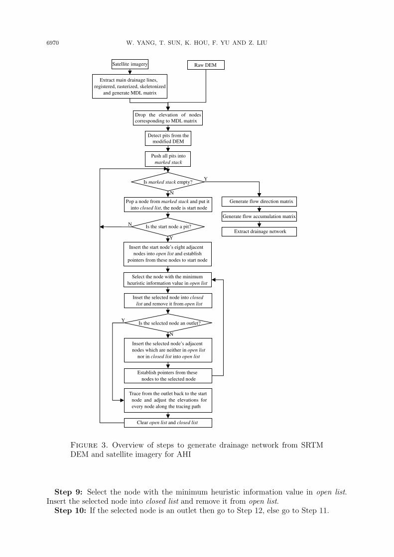
3.2. Proposed approach (AHI). Figure 3 shows a workflow of AHI. The main purposeof AHI is to process depressions and flat areas with heuristic information in one procedure,so both the depressions and flat areas are called pits. AHI requires three extra datastructures, a “closed list”, an “open list” and a “marked stack”. They are initially empty.The closed list stores the checked nodes, the open list keeps the unchecked nodes, and themarked stack stores the pits. The basic workflow includes the following steps and will bediscussed in detail in next section.

Step 1: Extract main drainage line from satellite imagery (the red line in Figure 2).Step 2: The main drainage line is registered, rasterized at the resolution of the DEM

and skeletonized [10,25] so as to make sure that it is one node thick. Then, generatingmain drainage line (MDL) matrix (the corresponding nodes of MDL matrix are set oneand the others are set zero).

Step 3: Drop the elevation of the corresponding nodes, whose values in MDL matrixare one, to some suitable values in order to increase flow accumulation value of thesenodes. In this study, the elevation of these nodes are decreased by 20%.

Step 4: Detect pits from the modified DEM and push them into marked stack.Step 5: If the marked stack is empty then go to Step 14, else go to Step 6.Step 6: Pop a node from marked stack and put it into closed list, the node is start

node.Step 7: If the start node is a pit then go to Step 8, else go to Step 5.Step 8: Inset the start node’s eight adjacent nodes into open list and establish pointers

from these nodes to the start node.


Is marked stack empty?

Satellite imagery Raw DEM

Push all pits into

marked stack

Drop the elevation of nodes

corresponding to MDL matrix

Detect pits from the

modified DEM

Pop a node from marked stack and put it

into closed list, the node is start node

N

Y

Is the start node a pit?

Y

Insert the start node’s eight adjacent

nodes into open list and establish

pointers from these nodes to start node

Select the node with the minimum

heuristic information value in open list

Inset the selected node into closed

list and remove it from open list

Is the selected node an outlet?

Insert the selected node’s adjacent

nodes which are neither in open list

nor in closed list into open list

N

Trace from the outlet back to the start

node and adjust the elevations for

every node along the tracing path

Clear open list and closed list

Generate flow direction matrix

Generate flow accumulation matrix

Extract drainage network

Y

N

Establish pointers from these

nodes to the selected node

Extract main drainage lines,

registered, rasterized, skeletonized

and generate MDL matrix

Figure 3. Overview of steps to generate drainage network from SRTMDEM and satellite imagery for AHI

Step 9: Select the node with the minimum heuristic information value in open list.Insert the selected node into closed list and remove it from open list.Step 10: If the selected node is an outlet then go to Step 12, else go to Step 11.


Step 11: Insert the selected node’s adjacent nodes which are neither in open list norin closed list into open list. Establish pointers from these nodes to the selected node thengo to Step 9.

Step 12: Trace from the outlet back to the start node and adjust the elevations forevery node along the tracing path.

Step 13: Clear open list and closed list, go to Step 5.Step 14: Generate flow direction matrix. The flow direction for a node is computed

based on the natural law that surface water flow will be directed to the steepest downslopedrop.

Step 15: Generate flow accumulation matrix. Each node in flow accumulation matrixrepresents the sum of the weights of all nodes in the matrix which drain to that node. Ifthe weights of all nodes are set one, then the resulting values of the flow accumulationmatrix will give the total contributing drainage area, in number of nodes. Other weightmatrices can be used for specific drainage related applications. In this study, the weightsof all nodes are set one.

Step 16: Extract drainage network. Flow accumulation matrix can be used to producedrainage network when nodes with values greater than an assigned constant thresholdvalue are selected. In this study, the constant threshold is 500.

3.2.1. Detecting pits. A 3×3 moving window is used over the raw DEM matrix to detectthe pits. The elevation difference (∆E) from the center node (E0) to one of its eightneighbours (Ei) is calculated as,

∆E =E0 − Ei

ϕ(i)(1)

where ϕ(i) = 1 for E, S, W and N neighbours and ϕ(i) =√2 for NE, SE, SW and NW

neighbours. Equation (1) can also be used to assign flow direction of nodes. If ∆E is lessthan zero, a zero flow direction is assigned to indicate that the flow direction is undefined.If ∆E is greater than zero and occurs at one neighbour, the flow direction is assignedto that neighbour. If ∆E is greater than zero and occurs at more than one neighbour,the flow direction is assigned to the maximum of ∆E (the lowest neighbour node). If theflow direction is still undefined, a zero flow direction is assigned to indicate that the flowdirection is undefined. The nodes with an undefined flow direction are pits and will beprocessed using the heuristic information.

3.2.2. Generating MDL matrix. Extract main drainage line from satellite imagery (thered line in Figure 2). Due to the topographical characteristics, the main drainage lineis delineated from satellite imagery using visual interpretation. The drainage paths arecharacterized by higher soil moisture content. This gives clear dark tone all along thedrainage line in the study area. This is also verified from the field observation. MDL isregistered, rasterized at the resolution of the DEM and skeletonized [10,25] so as to makesure that it is one node thick. The result is stored in MDL matrix.

3.2.3. Finding the optimal outlet of pits. While searching for outlet of a pit, the methodsdescribed above check the eight adjacent nodes and rarely considered the general trendof the DEM. In other words, they have no additional information about states beyondthat provides in the problem definition. All they can do is to generate successors anddistinguish a goal state from a nongoal state. These methods can find the outlets, butthey are probably incredible and inefficient in most cases. Unrealistic parallel drainagelines, unreal drainage lines and spurious terrain features are most likely to be generated.


Heuristic information about the state space can prevent algorithms from blunderingabout in the dark [36]. AHI uses the heuristic information to find the optimal outlet.AHI executes a single searching procedure on every pit. The searching procedure tries

to find the outlet of a pit. It can be regarded as a path searching problem. Start is a pitand goal is an outlet of the pit. AHI uses heuristic information value to evaluate node ion searching path, according to,

HI(i) =

α× ELEVi + β × ∥L(s, i)∥+ γ ×

∑k∈SETi

ELEVk

| SETi |+ θ ×MINi,

i /∈ MDL

α× ELEVi × (1−▽) + β × ∥L(s, i)∥+ γ ×

∑k∈SETi

ELEVk

| SETi |+ θ ×MINi,

i ∈ MDL

(2)

In addition to Equation (2), we also have,

MINi = min{ELEVm | m ∈ SETi,m /∈ open list,m /∈ closed list} (3)

Equations (2) and (3) together describe heuristic information function of AHI. WhereHI(i) is heuristic information value of node i. α×ELEVi+β×∥L(s, i)∥ is actual cost ofnode i when the value of node i in MDL matrix is zero (i /∈ MDL), and α×ELEVi× (1−▽)+β×∥L(s, i)∥ is actual cost of node i when the value of node i in MDL matrix is one(i ∈MDL). ELEVi is the elevation value of node i. ∥L(s, i)∥ is the path length from s toi (the path length of two adjacent nodes is 1 for E, S, W and N neighbours or

√2 for NE,

SE, SW and NW neighbours), and s is start node (a pit). γ×

∑k∈SETi

ELEVk

| SETi |+ θ×MINi

is estimated cost of node i.

∑k∈SETi

ELEVk

| SETi |is the arithmetic average elevation of the nodes

in n×n (n = 3, 5, 7, · · · ) window centered node i (in this study, n = 5), SETi is a setwhich contains all nodes in n×n window centered the node i, k is a element of SETi, and| SETi | is the number of nodes in SETi. MINi is the minimum elevation value of nodem in SETi and m is neither in open list nor in closed list. α, β, γ and θ are weightingfactors, based on the priority (p) of the four factors. The weighting value can be expressedusing 2p, where the higher the priority, the larger the weighting value. In this study, thecorresponding weighting factors for α, β, γ and θ are 23, 20, 21 and 23. ▽ is to decreaseheuristic information value of the node i when the value of node i in MDL matrix (i ∈MDL) is one. In this study, ▽ is 0.2.AHI is initialized by pop a node from marked stack and put it into closed list, which

thereby becomes the start node for one searching procedure of AHI. In turn, the node withthe minimum heuristic information value is removed from open list and added into closedlist, and its adjacent nodes which are neither in open list nor in closed list are added intoopen list. The iteration continues until a selected node in open list satisfies the terminatingcriteria, which is an outlet node for the drainage. The terminating criteria require thenode with the minimum heuristic information value and it has a lower elevation than thestart node. Finally, Trace from the outlet back to the start node and adjust the elevations


for every node along the tracing path to create a gradient according to Equation (4),

ELEVi(new) = ELEVs − (ELEVs − ELEVo)×∥L(s, i)∥∥L(s, o)∥

(4)

where ELEVs is elevation value of start node s, ELEVo is elevation value of outlet node o,ELEVi is elevation value of node i, ELEVi(new) is new elevation value of the node i afteradjusted. When all pits are processed, we can get the flow direction matrix. Using theflow direction matrix as input, the flow accumulation matrix is determined. The drainagenetwork can be extracted from the flow accumulation matrix by specifying a constantthreshold.

4. Experimental Results and Analysis. To examine the suitability and performanceof AHI, we implement it in C and make experiments on the study area. For presentationpurpose all raster maps are converted into vector format.

There is no standard method to assess the quality of delineated network. Networks aredifficult objects to compare quantitatively [38]. Although, we compare AHI to one of theexisting methods, Agree. Agree is implemented with the Arc Hydro tools. The Arc Hydrotools are a set of public domain utilities developed jointly by the Center for Research inWater Resources (http://www.crwr.utexas.edu) of the University of Texas at Austin, andthe Environmental Systems Research Institute, Inc. These tools provide functionalitiesfor terrain processing, watershed delineation and attribute management. They operateon top of the Arc Hydro data model in the ArcGIS 8.3, 9.0, 9.1, 9.2 and 9.3 environments.

Figure 4. Extraction result of Agree (threshold = 500)

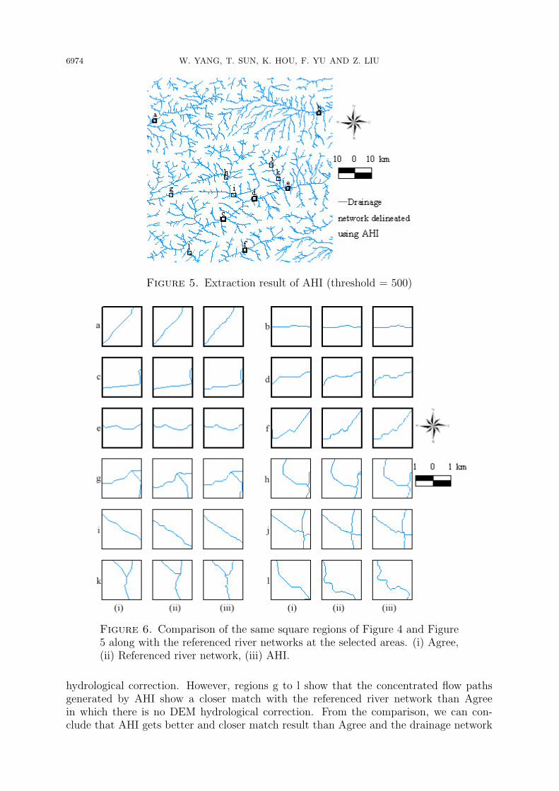
Figure 4 and Figure 5 show the drainage networks generated by Agree and AHI. It isobvious that the major drainage could be delineated satisfactorily by the two methods.Extraction results produced by Agree and AHI look alike. We select 12 square regions(a to l in Figure 4 and Figure 5) where the differences are more visible. Some nodes’elevation values in regions a to f (wide line square regions) are corrected by MDL matrix,while all nodes’ elevation values in regions g to l (narrow line square regions) are notcorrected.

Figure 6 shows the detail from the same square regions of Figure 4 and Figure 5 alongwith the referenced river network at selected areas. It can be seen from regions a to f thatAgree and AHI have produced very similar results to each other in which there is DEM


Figure 5. Extraction result of AHI (threshold = 500)

Figure 6. Comparison of the same square regions of Figure 4 and Figure5 along with the referenced river networks at the selected areas. (i) Agree,(ii) Referenced river network, (iii) AHI.

hydrological correction. However, regions g to l show that the concentrated flow pathsgenerated by AHI show a closer match with the referenced river network than Agreein which there is no DEM hydrological correction. From the comparison, we can con-clude that AHI gets better and closer match result than Agree and the drainage network


produced by AHI is more reasonable whether there is DEM hydrological correction ornot.

The comparison and analysis mentioned above is local, visual and qualitative betweenthe two methods and the global, objective, quantitative comparison and analysis will bementioned below.

Table 1. Summary of elevation modified by Agree and AHI (The mostsuccessful method is identified in bold).

MethodNumber of nodes Percentage of nodes Sum of elevation

modified modified modified (abs m)Agree 71353 4.96% 4330092AHI 17425 1.21% 3684214

The number of nodes corrected by the two methods is presented in Table 1. AHIcorrected fewer nodes than Agree. These results are reflected also in the sum of theelevation differences between the raw DEM and the corrected DEM after processing allpits and flat areas. The less values of the raw DEM are corrected, the more terrainfeatures are retained.

In order to measure the distance between the referenced river network and each drainagenetwork, we create buffers around the referenced river network at distance multiple of5×10−4 decimal degrees (see Figure 7). The middle line in Figure 7 is the referenced rivernetwork. 5×10−4 decimal degrees distance around the referenced river network is denotedby “buffer 5”(or “a”) and 10×10−4 is denote by “buffer 10”(or “b”) and so forth.

In order to measure the distance between MDL and each drainage network, we alsocreate the same buffers around the MDL.

Table 2. Percent of nodes in the different buffer areas around the MDLfor Agree and AHI. The size of buffers is in 10−4 decimal degrees for eachside of the MDL (The most successful method is identified in bold).

XXXXXXXXXXXMethodBuffer size

5 10 15 20 25 30 35 40 45 50

Agree12.91 13.98 14.30 14.61 14.92 15.22 15.53 15.84 16.16 16.52% % % % % % % % % %

AHI13.62 13.97 14.35 14.79 15.17 15.53 15.94 16.33 16.73 17.10% % % % % % % % % %

Table 3. Percent of nodes in the different buffer areas around the refer-enced river network for Agree and AHI. The size of buffers is in 10−4 decimaldegrees for each side of the referenced river network (The most successfulmethod is identified in bold).

XXXXXXXXXXXMethodBuffer size

5 10 15 20 25 30 35 40 45 50

Agree25.29 36.13 44.37 50.50 54.55 57.13 58.87 60.13 61.16 62.12% % % % % % % % % %

AHI27.34 39.69 48.02 53.36 56.44 58.31 59.64 60.71 61.69 62.62% % % % % % % % % %


a b c ed f h i k 2

Figure 7. Zoom on buffered referenced river network

The spatial positioning of the extracted drainage network is accessed by calculating thenumber of nodes of the two networks falling in the different buffer areas normalized by thetotal number of nodes for each drainage network. Results around the MDL are presentedin Table 2 and results around the referenced river network are presented in Table 3. FromTable 2, it can be seen that the two methods fall in the different buffer areas with similarpercent of nodes around the MDL. However, Table 3 shows that Less than 28% of thenodes of the extracted drainage networks are contained in the smallest buffer size. Thevalues are then regularly growing up to a maximum of 63%. It is obvious that the morenodes are in the same smaller buffer area, the closer the method is to the referenced rivernetwork. It can be concluded from Table 3 that the spatial positioning of the drainagenetwork extracted by AHI is closer to the ground truth network in each buffer area thanAHI.

5. Conclusions and FutureWork. DEMs are an important tool for spatially modellinghydrology and DEM hydrological correction is often required to improve their represen-tation of true hydrology when DEM of sufficient resolution and accuracy does not existor high-resolution DEM is available in low-relief areas. In this paper, we use the girdSRTM DEM and satellite imagery data for extracting drainage network to compensatefor the weaknesses of DEMs. The limitation of node numbers is mainly determined bythe capacity of computer’s memory. The largest dataset that we have made an experi-ment with is size of 6000×4800. The experiments were carried on a computer with 1GBRAM, which included about 400MB occupied by the OS. The entire drainage network


delineated procedure is carried out by a single program coded in C. We have tested ourtechnique on SRTM DEM and satellite imagery, sub-scene of an area located in the mid-dle of Afghanistan. The experimental evidence suggests that AHI can extract drainagenetwork better and fully than Agree. From the comparison and analysis of the drainagenetworks generated by AHI and Agree, it can be concluded that the extracted drainagenetwork by AHI cannot be entirely matched with the referenced river network but AHIshows a closer match and get better result than Agree whether there is DEM hydrologicalcorrection or not. Our future research is adding affecting factor of rainfall, soil, vegetationand others to the heuristic information function. We believe that a much closer matchresult may be obtained.

Acknowledgment. This research is sponsored by Jilin Provincial Science and Technol-ogy Department of P. R. China, under the Grant Number 20090503, the Special Fund forFast Sharing of Science Paper in Net Era by CSTD of the Ministry of Education of P. R.China, under the Grant Number 20090043110010, Jilin Provincial Education Departmentof P. R. China, under the Grant Number 2009587 and the Fundamental Research Fundsfor the Central Universities, under the Grant Number 09QNJJ007, respectively. We wouldlike to thank these organizations for their great support to our research. The authors alsogratefully acknowledge the helpful comments and suggestions of the reviewers, which haveimproved the presentation.

REFERENCES

[1] I. D. Moore, R. B. Grayson and A. R. Ladson, Digital terrain modeling: A review of hydrological,geomorphological and biological applications, Hydrological Processes, vol.5, pp.1-42, 1991.

[2] G. E. Moglen and R. L. Bras, The importance of spatially heterogeneous erosivity and the cumulativearea distribution within a basin evolution model, Geomorphology, vol.12, pp.173-185, 1995.

[3] M. L. Lin and C. W. Chen, Using GIS-based spatial geocomputation from remotely sensed data fordrought risk-sensitive assessment, International Journal of Innovative Computing, Information andControl, vol.7, no.2, pp.657-668, 2011.

[4] L. H. Lee, M. J. Huang, S. W. S. H. Yue and C. Y. Lin, An adaptive filtering and terrain recoveryapproach for airborne lidar data, International Journal of Innovative Computing, Information andControl, vol.4, no.6, pp.1783-1796, 2008.

[5] C. Qin, A. X. Zhu, T. Pei, B. Li, C. Zhou and L. Yang, An adaptive approach to selecting a flow-partition exponent for a multiple-flow-direction algorithm, International Journal of GeographicalInformation Science, vol.21, no.4, pp.443-458, 2007.

[6] J. Hogg, J. E. McCormack, S. A. Roberts, M. N. Gahegan and B. S. Hoyle, Automated derivationof stream-channel networks and selected catchment characteristics from digital elevation models, inGeographical Information Handling: Research and Applications, Chichester, Wiley, 1997.

[7] D. R. Maidment, GIS and hydrologic modeling, in Environmental Modeling With GIS, New York,Oxford University Press, 1993.

[8] Editors of ESRI Press, ArcGIS Desktop Developers Guide: ArcGIS 9, ESRI Press, 2004.[9] M. Neteler and H. Nitasova, Open Source GIS: A GRASS GIS Approach, 2nd Edition, Kluwer,

Dordrecht, the Netherlands, 2004.[10] M. Emilio, G. L. Miles, V. R. B. Maria and E. R. Jeffrey, Estimating cell-to-cell land surface drainage

paths from digital channel networks, with an application to the Amazon basin, Journal of Hydrology,vol.315, pp.167-182, 2005.

[11] F. Kenny, B. Matthews and K. Todd, Routing overland flow through sinks and flats in interpolatedraster terrain surfaces, Computer and Geosciences, vol.34, pp.1417-1430, 2008.

[12] M. J. Oimoen, An effective filter for removal of production artifacts in us geological survey 7.5-minute digital elevation models, Proc. of the 14th International Conference on Applied GeologicRemote Sensing, pp.311-319, 2000.

[13] J. Lindsay and I. F. Creed, Sensitivity of digital landscapes to artifact depressions in remotely-sensedDEMs, Photogrammetric Engineering and Remote Sensing, vol.71, pp.1029-1036, 2005.


[14] J. F. O’Callaghan and D. M. Mark, The extraction of drainage networks from digital elevation data,Computer Vision, Graphics, and Image Processing, vol.28, pp.323-344, 1984.

[15] L. E. Band, Topographic partition of watersheds with digital elevation models, Water ResourcesResearch, pp.15-24, 1986.

[16] Z. Qing, X. T. Yi and Z. Jie, A efficient depression processing algorithm for hydrologic analysis,Computers and Geosciences, vol.32, pp.615-623, 2006.

[17] L. W. Martz and J. Garbrecht, Automated extraction of drainage network and watershed data fromdigital elevation models, Water Resources Bulletin, vol.29, pp.901-908, 1993.

[18] S. K. Jenson and J. O. Domingue, Extracting topographic structures from digital elevation datafrom geographic information system analysis, Photogrammetric Engineering and Remote Sensing,vol.54, pp.1593-1600, 1988.

[19] L. W. Martz and D. E. Jong, CATCH: A FORTRAN program for measuring catchment area fromdigital elevation models, Computers and Geosciences, vol.14, no.5, pp.627-640, 1988.

[20] A. Tribe, Automated recognition of valley lines and drainage networks from grid digital elevationmodels: A review and a new method, Journal of Hydrology, vol.139, no.1-4, pp.263-293, 1992.

[21] R. Turcotte, J. P. Fortin, A. N. Rousseau, S. Massicotte and J. P. Villeneuve, Determination ofthe drainage structure of a watershed using a digital elevation model and a digital river and lakenetwork, Journal of Hydrology, vol.240, pp.225-242, 2001.

[22] N. C. John, P. V. N. Kimberly and S. B. Guy, How does modifying a DEM to reflect known hydrologyaffect subsequent terrain analysis, Journal of Hydrology, vol.332, pp.30-39, 2007.

[23] W. Saunders, Preparation of DEMs for use in environmental modeling analysis, 1999 ESRI UserConference, ESRI Online, San Diego, CA, 1999.

[24] P. Doll and B. Lehner, Validation of a new global 30-min drainage direction map, Journal of Hy-drology, vol.258, no.1-4, pp.214-231, 2002.

[25] P. Soille, J. Vogt and R. Colombo, Carving and adaptive drainage enforcement of grid digital eleva-tion models, Water Resour. Res., vol.39, no.12, pp.1366-1379, 2003.

[26] D. R. Maidment, GIS and hydrological modelling: An assessment of progress, The 3rd InternationalConference on GIS and Environmental Modelling, Santa Fe, NM, pp.20-25, 1996.

[27] P. J. Mizgallewicz and D. Maidment, Modelling agricultural transport in midwest rivers using geo-graphic information systems, Center for Research Water Resources Online Report 96-6, Universityof Texas, Austin, TX, 1996.

[28] R. Hellweger, Agree.aml, Center for Research in Water Resources, The University of Texas at Austin,Austin, TX, 1996.

[29] F. L. Hellweger, AGREE – DEM Surface Reconditioning System, http://www.ce.utexas.edu/prof/maidment/ gishydro/ferdi/research/agree/agree.html, 1997.

[30] A. M. Quenzer and D. R. Maidment, A GIS assessment of the total loads and water quality in thecorpus Christi Bay system, Center for Research in Water Resources Online Report 98-1, Universityof Texas, Austin, TX, 1998.

[31] M. F. Hutchinson, A locally adaptive approach to the interpolation of digital elevation models, The3rd International Conference/Workshop on Integrating GIS and Environmental Modeling, NationalCenter for Geographic Information and Analysis, University of California, Santa Barbara, 1996.

[32] M. F. Hutchinson, ANUDEM Version 4.6.2, http://cres.anu.edu.au/software/anudem.html, 1998.[33] L. L. Yun and K. C. Uchimura, Using self-organizing map for road network extraction from IKONOS

imagery, International Journal of Innovative Computing, Information and Control, vol.3, no.3,pp.641-656, 2007.

[34] I. K. Ku, Z. S. Li and C. H. Xu, Solving large multilevel lot-sizing problems with a simple heuristicalgorithm based on segmentation, International Journal of Innovative Computing, Information andControl, vol.6, no.3(A), pp.817-827, 2010.

[35] A. Jarvis, H. I. Reuter, A. Nelson and E. Guevara, Hole-filled Seamless SRTM Data V4,http://srtm.csi.cgiar.org, 2008 (accessed 13 October 2009).

[36] USAID (United States Agency for International Development), AIMS (Afghanistan InformationManagement Service), http://www.aims.org.af, 1990 (accessed 13 October 2009).

[37] S. J. Russel and P. Norvig, Artificial Intelligence – A Modern Approach Pearson Education, NewJersey, 2003.

[38] I. Molly and T. F. Stepinski, Automatic mapping of valley networks on Mars, Computers and Geo-sciences, vol.33, no.6, pp.728-738, 2007.

an adaptive approach for extraction of drainage network

Documents