an adaptive coupled level-set/volume-of-ﬂuid interface...

Journal of Computational Physics 217 (2006) 364–394

www.elsevier.com/locate/jcp

An adaptive coupled level-set/volume-of-fluidinterface capturing method for unstructured triangular grids

Xiaofeng Yang a, Ashley J. James a,*, John Lowengrub b,Xiaoming Zheng b, Vittorio Cristini c

a Department of Aerospace Engineering and Mechanics, University of Minnesota, 107 Akerman Hall, 110 Union St SE,

Minneapolis, MN 55455, USAb School of Mathematics, University of California, Irvine, USAc Biomedical Engineering, University of California, Irvine, USA

Received 10 January 2005; received in revised form 4 January 2006; accepted 5 January 2006Available online 2 March 2006

Abstract

We present an adaptive coupled level-set/volume-of-fluid (ACLSVOF) method for interfacial flow simulations onunstructured triangular grids. At each time step, we evolve both the level set function and the volume fraction. The levelset function is evolved by solving the level set advection equation using a discontinuous Galerkin finite element method.The volume fraction advection is performed using a Lagrangian–Eulerian method. The interface is reconstructed based onboth the level set and the volume fraction information. In particular, the interface normal vector is calculated from thelevel set function while the line constant is determined by enforcing mass conservation based on the volume fraction. Dif-ferent from previous works, we have developed an analytic method for finding the line constant on triangular grids, whichmakes interface reconstruction efficient and conserves volume of fluid exactly. The level set function is finally reinitializedto the signed distance to the reconstructed interface. Since the level set function is continuous, the normal vector calcula-tion is easy and accurate compared to a classic volume-of-fluid method, while tracking the volume fraction is essential forenforcing mass conservation. The method is also coupled to a finite element based Stokes flow solver. The code validationshows that our method is second order and mass is conserved very accurately. In addition, owing to the adaptive grid algo-rithm we can resolve complex interface changes and interfaces of high curvature efficiently and accurately.� 2006 Elsevier Inc. All rights reserved.

Keywords: VOF; Level set; Interface; Unstructured grid

1. Introduction

Flows involving two or more different fluids are very common in many natural and industrial processes, forexample, rain drops in the air, free surface flows in the ocean, the dispersion of two immiscible fluids into each

0021-9991/$ - see front matter � 2006 Elsevier Inc. All rights reserved.

doi:10.1016/j.jcp.2006.01.007

* Corresponding author. Tel.: +1 612 625 6027; fax: +1 612 626 1558.E-mail address: [email protected] (A.J. James).

mailto:[email protected]

X. Yang et al. / Journal of Computational Physics 217 (2006) 364–394 365

other to create emulsions, polymer blending, and so on. Numerical simulations of such flows are difficultbecause the interface separating different fluid phases must be accurately tracked or captured simultaneouslywith the flow field evolution. Many methods have been developed for this purpose in the last two decades.Typical methods are the marker particle (MP) method [1], the level set (LS) method [2–4], the volume-of-fluid(VOF) method [5–7], the front tracking method [8,9], and the phase field method [10–14]. Each of these meth-ods has its own advantages and disadvantages, and has been developed into various versions with steadyimprovements. A detailed introduction and a comparison study of several variants of the MP method, theLS method, and the VOF method were given by Rider and Kothe [15].

In an LS method, the interface is captured by a level set function /, which is zero on an interface, is positivein one fluid and is negative in the other fluid. The interface is thus represented by the zero level sets. The levelset function is advected by the velocity u of the flow field as

/t þ u � r/ ¼ 0. ð1Þ

Usually, / is initialized as a signed distance from each grid point to the interface, and it is desirable to maintain/ as a signed distance function as the interface evolves since, otherwise, high gradients or even a jump in / candevelop, for example, when interfaces merge. The high gradients in / could result in excessive errors when, forexample, derivatives of / are taken to find the interface normal vectors. In addition, maintaining / as a dis-tance function is important for providing the interface a width fixed in time [16,17] because in numerical imple-mentations the discontinuous surface delta function in the surface tension force term needs to be smoothedover a finite, but small width to avoid numerical instability, and the measure of the width is based on the levelset function, which is assumed to be a signed distance function. However, when / is advected according to Eq.(1), it does not remain a distance function in general. Therefore, a redistancing or reinitialization procedure isneeded to modify the advected level set function such that the modified level set function is a signed distancefunction while the zero level sets remain the same before and after the redistancing, that is, the interface re-mains unchanged during the redistancing. Notable previous works on redistancing have been done by Suss-man and his coworkers [17,18]. Their previous paper [16] also provides a profound understanding of theirworks. A review of the LS method with an emphasis on applications in fluid interfaces was given by Sethianand Smereka [3]. See also Osher and Fedkiw [4]. The advantage of an LS method is that it handles mergingand breaking of the interface automatically, the interface never has to be explicitly reconstructed, and since /is a smooth function, the unit normal n and curvature j of the interface can be easily calculated from / as

n ¼ r/jr/j and j ¼ r � n. ð2Þ

A well-known drawback of the LS method is mass loss/gain, i.e., the mass (or volume for incompressible flow)of the fluid is not conserved. For example, in a drop collision simulation the average mass error with themethod described in [18] is 0.5% and the error with the method described in [16] is 1.3%. Even though the zerolevel sets of / can remain unchanged with some order of accuracy during the redistancing, the volumeenclosed by the zero level sets is not conserved as / evolves according to Eq. (1). An open problem is to findmore conservative schemes to solve (1) [18].

In the VOF method, a volume fraction function f is defined. The value of the volume fraction in each gridcell is equal to the ratio of the volume of one of the fluids in this cell, called fluid 1, to the total volume of thegrid cell. Thus, f is unity in a cell that lies completely in fluid 1, and is zero if the cell lies completely in the otherfluid, called fluid 2. For cells that include an interface (called the interfacial cells), and thus contain both fluid 1and fluid 2, f is between zero and unity. Inversely, given the volume fraction in each grid cell, one can recon-struct an approximate interface, which is called ‘‘interface reconstruction’’. The f field is advected by the flowfield, that is

ft þ u � rf ¼ 0. ð3Þ

However, meaningful solution of Eq. (3) is not easy. Because f is a discontinuous function, using standardnumerical schemes such as an upwind finite difference method to solve Eq. (3) can easily diffuse the interface,which should, however, remain sharp. One way to overcome this problem is to advect f based on a recon-structed interface determined by the f field. Interface reconstruction is thus a key part of any VOF method,

366 X. Yang et al. / Journal of Computational Physics 217 (2006) 364–394

and has been improved from the original simple line (piecewise constant) interface reconstruction (SLIC) topiecewise linear interface reconstruction (PLIC). A detailed review of some SLIC and PLIC interface recon-struction methods from a historical perspective was given by Rider and Kothe [6]. Piecewise circle [19], piece-wise parabolic [20,21], and piecewise spline [22] interface reconstructions have also been developed. Two newinterface reconstruction methods based on a least squares fit were presented by Scardovelli and Zaleski [23].Based on the reconstructed interface, several schemes have been developed to advect f. Most of these worksare based on Eulerian advection of f on structured grids, either with a split scheme or an unsplit scheme. Thesekind of schemes are described by Rider and Kothe [6]. However, the implementation of these schemes on tri-angular unstructured grids is difficult. In particular, it is very complicated to compute the fluid volume fluxesfor triangular cells. A promising method is the Lagrangian–Eulerian advection method, which consists ofthree typical stages: a Lagrangian projection, an interface reconstruction, and a remapping. This method isindependent of the grid type. It is suitable for both rectangular structured grids and triangular unstructuredgrids. Typical works on this method are Shahbazi et al. [24] and Ashgriz et al. [25]. A new mixed split Eulerianimplicit—Lagrangian explicit advection scheme was presented by Scardovelli and Zaleski [23].

Compared to the LS method, a notable merit of the VOF method is that it can conserve mass very accu-rately. A drawback of the VOF method is that it is hard to compute accurate interface normals and curvaturesbecause of the discontinuity in f. Several algorithms have been developed for normal vector calculations. How-ever, most of them are less than second order accurate. A detailed comparison of several normal calculationmethods was given by Rider and Kothe [6]. Calculations of curvature are even more difficult because theyinvolve taking second order derivatives of f. Usually, the f field is smoothed by some kernel function whenused for curvature calculations. However, the optimum type and extent of the kernel operation may very welldepend on the interfacial flow being modeled [26]. A detailed comparison of several kernels and some princi-ples on how to choose a kernel function were given by Williams et al. [27].

Recently, methods that couple two different schemes have been developed. Examples are the coupled levelset and volume-of-fluid method (CLSVOF) [28,29], the hybrid particle level set method [30], and the mixedmarkers and volume-of-fluid method [31]. A coupled method takes advantage of the strengths of each ofthe two methods, and is therefore superior to either method alone. In a CLSVOF method, both / and f

are evolved according to Eqs. (1) and (3), respectively. / is used to calculate the unit normal and curvatureof the interface. f, together with the unit normal calculated from /, is used to reconstruct a new interface.Thus, / can finally be reset to a signed distance function based on the reconstructed interface. Volume canbe conserved very accurately by tracking f. Since / is continuous, the calculation of the interface normaland curvature is natural, easy and accurate, in contrast to the normal and curvature calculation in a pureVOF method, which requires unphysical smoothing of f. However, most of the previous works, includingthe CLSVOF method by Sussman and Puckett [28], are for structured grids. A few works have been doneon unstructured grids [24,25,32,19]. Very recently, Sussman et al. [33,34] have developed a CLSVOF methodfor an adaptive Cartesian grid.

The goal of the present paper is to present an adaptive coupled level set and volume-of-fluid (ACLSVOF)volume tracking method for unstructured triangular grids. Using adaptive unstructured grids, we can clusterthe grid near the interface, enabling us to efficiently and accurately resolve complex changes in interface topol-ogy, regions of high interface curvature, and the near contact regions between two impacting interfaces, whichis in general hard to achieve on structured grids. In our work, we use the adaptive mesh algorithm developedin [35,36], which is based on the earlier work of Cristini et al. [37]. For the advection of the level set function,we solve Eq. (1) using a discontinuous Galerkin finite element method. For the evolution of the volume frac-tion, we use a Lagrangian–Eulerian advection scheme. Different from the works by Shahbazi et al. [24] andAshgriz et al. [25], our algorithm for volume fraction advection is built in the framework of our ACLSVOFmethod, where the normal and the curvature of the interface will be calculated from the continuous level setfunction. For interface reconstruction, different from the previous works, we have developed an analytic piece-wise linear interface reconstruction for triangular grids [38]. The method is also coupled to a finite elementbased Stokes solver. We use the Stokes solver for illustration. The method can be generalized to Navier–Stokes and viscoelastic flows. Solid body translation, rotation, Zalesak disk rotation and a single vortex flowproblem are simulated to test our ACLSVOF volume tracking method. Drop deformation in an extensionalflow is simulated with the volume tracking method coupled to the Stokes solver.


The rest of the paper is organized as follows. In Section 2 we describe the numerical methods for the levelset function evolution, the volume fraction evolution, grid adaption, and the Stokes flow solver. Code valida-tion and results are presented in Section 3. A conclusion is given in Section 4.

2. Computational methods

2.1. The Eulerian evolution of the level set function

The evolution of the level set function is governed by Eq. (1). In practice, we reformulate Eq. (1) as

/t þr � ðu/Þ ¼ /r � u. ð4Þ
Theoretically, we have $ Æ u = 0 for incompressible flow. Numerically, however, this is not true in general. So,the right hand side is retained in Eq. (4) such that the level set function is only convected by the velocity fieldeven when the numerical velocity field is not exactly divergence free.
Eq. (4) is solved using a Runge–Kutta discontinuous Galerkin finite element method (RKDG) [39,40]on a fixed Eulerian grid (in contrast to the projected Lagrangian grid used in the next section). See also[36]. Let P1(T) be the set of all polynomials of degree at most 1 on the triangular element T, and Th atriangulation of the computational domain X with a characteristic grid size h. The finite element space isdefined as

W h ¼ fv 2 L2ðXÞ : vjT 2 P 1ðT Þ; 8T 2Thg. ð5Þ
Then, our numerical method is to find an approximate solution /h 2Wh, such that in each element T 2Th Z
T

o/h

otv�

ZT

/huh � rvþXe2oT

Ze

uh � n/hv� ¼Z

Tr � u/hv; 8v 2 P 1ðT Þ; ð6Þ

where uh is the discrete velocity, v� denotes the value of a test function taken from within element T, /h is asingle-valued flux through an element boundary e, and n is the outward unit normal of T. Note that uh is con-tinuous across any element boundary (we employ a continuous velocity space; see Section 2.4.), but /h and thetest function v are discontinuous across an element boundary. Specifically, /h is defined as,

/h ¼/�h if uh � n P 0;

/þh if uh � n < 0;

�ð7Þ

where /�h is the value of /h on boundary e taken from within element T, and /þh is the value of /h on boundarye taken from outside element T.

The time integration is performed using a second order Runge–Kutta scheme. For efficiency, the narrowband/local level set strategy is utilized so that Eq. (6) is solved only in the neighborhood of the interface(see also [36]).

Since the numerical level set function /h obtained from the above discontinuous Galerkin method is dis-continuous, we project (in the L2 sense) the discontinuous /h onto a continuous piecewise linear space beforewe use it to calculate the interface normal vector. Specifically, we define the continuous piecewise linear spaceas

W �h ¼ fv 2 C0ðXÞ \ L2ðXÞ : vjT 2 P 1ðT Þ; 8T 2Thg. ð8Þ

Let /�h denote the continuous level set function obtained by the projection. Then, the L2 projection of /h 2Wh

to /�h 2 W �h is simply the solution of the following weak formulation:
Z
X/�hv ¼

ZX

/hv; 8v 2 W �h. ð9Þ

In the framework of our ACLSVOF method, this continuous level set function will be used for interface nor-mal calculations during interface reconstruction, and for convenience the superscript * will be omitted fromnow on. At the end of each time step, the level set function will be reinitialized to a signed distance functionbased on the reconstructed interface.


2.2. The Lagrangian–Eulerian volume fraction evolution

For the volume fraction advection, we employ a Lagrangian–Eulerian advection scheme, which consists ofthree stages: a Lagrangian projection stage, a reconstruction stage, and a remapping stage. Similar works canbe found in [24,25]. Fig. 1 shows a schematic of the method. During the Lagrangian projection stage, we treateach grid cell as a material element. All fluid elements (or equivalently the grid cells) are advected/projectedusing a Lagrangian approach. For example, in Fig. 1, by projecting fluid element ABC we get the correspond-ing projected Lagrangian element A 0B 0C 0. Because the volume fraction is solely transported with the flow, thevolume fraction remains the same during the projection. Notice that for a linear velocity field triangles remaintriangles, no matter how they deform. All projected elements form a new grid, which we call the Lagrangiangrid. In contrast, the original grid is called the Eulerian grid.

As the shape of each element deforms, the interface position in each interfacial cell also changes. During thereconstruction stage, we reconstruct the interface on the Lagrangian grid. The interface is approximated usingpiecewise linear segments based on both the level set field and the volume fraction field. The reconstructedinterface concretely defines the configuration of each fluid phase on the Lagrangian mesh, as illustrated inFig. 1, where the two fluids in cell A 0B 0C 0 are separated by a reconstructed interface segment E 0F 0. A 0B 0E 0F 0

is full of fluid 1, and C 0E 0F 0 is full of fluid 2. Based on this information, we map each fluid element on theLagrangian mesh back to the original Eulerian mesh (or an adapted mesh when the grid is remeshed) duringthe remapping stage, which gives us the advected volume fraction on the Eulerian grid and completes the vol-ume fraction advection. Details of the method are as follows.

2.2.1. Lagrangian volume fraction projection

The projection of the volume fraction is equivalent to solving the volume fraction advection equation (3)using a Lagrangian approach. Let us consider each grid cell a material element, and let f n

T be the volume frac-tion in element T at time tn, then we have from Eq. (3) discretely that

~f nþ1T ¼ f n

T ; 8T 2Th; ð10Þ
where ~f nþ1
T denotes the volume fraction in element T after a Lagrangian advection. Eq. (10) is equivalent tosaying that the volume fraction in each element is solely transported with the flow, which is consistent with thedifferential Eq. (3).

In the meantime, each material element transports with the flow. So, we have that

dx

dt¼ u; ð11Þ

A

B C

A’

B’

C’

E’

F’

∫udt

Fig. 1. Schematic of the Lagrangian–Eulerian volume fraction evolution.


where x is the location of a material point on the boundary of an element. Numerically, if we assume that thevelocity is piecewise linear over every finite element, then finding the Lagrangian position of each elementT 2Th is equivalent to finding the Lagrangian position of each vertex of T. This can be achieved by solvingEq. (11) at each vertex of the grid. These projected elements form a new projected grid that we call theLagrangian grid. Using a second order Runge–Kutta (RK) scheme, we can obtain the coordinates of each gridnode of the Lagrangian grid as the following

~xnþ1

2i ¼ xn

i þDt2

uðxni ; t

nÞ; for i ¼ 1; . . . ;MT ; ð12Þ

~xnþ1i ¼ xn

i þ Dtuð~xnþ1=2i ; tnþ1

2Þ; for i ¼ 1; . . . ;MT ; ð13Þ
where MT is the total number of grid nodes, and uð~xnþ1=2
i ; tnþ12Þ on the Lagrangian mesh has been interpolated

from the Eulerian mesh.In the first step of the RK integration a triangular Eulerian grid cell is projected using the linear velocity

field in that cell, so it remains a triangle, although it may deform. To perform the second step of the RK inte-gration, the velocity is updated on the Eulerian mesh, then interpolation is used to determine the velocity atthe vertices of the Lagrangian grid cells. It is assumed that these velocities define a linear velocity field in eachLagrangian cell, so that in this second RK step we are again projecting a triangle with a linear velocity field, soit remains a triangle. If the velocity field on the Eulerian mesh were used directly then cell edges would be pro-jected with a velocity field that is only piecewise linear, so the projected cell edges would be piecewise linear.

Theoretically, the above Lagrangian projection conserves the volume of fluid in each element, because thevolume of each element does not change due to the incompressibility of the fluid. Numerically, however, thevolume of fluid can not be exactly conserved, because: (i) the numerical velocity field delivered from a flowsolver is in general not exactly divergence free; (ii) the numerical velocity field is approximated by piecewiselinear basis functions, and a triangular element remains a triangle during a projection only for linear velocities;(iii) in the second RK step the velocity on the Lagrangian mesh is interpolated from the Eulerian mesh; and(iv) the numerical integration of Eq. (11) is, of course, not exact. In other words, because of these four reasons,the volume of a material element (or grid cell) is not exactly constant during the above numerical Lagrangianprojection, and thus, the volume of each single fluid phase may not be conserved exactly during the projection.

However, as we will show in Section 3, the volume loss/gain due to the last three reasons is extremely small.The magnitude of the volume loss/gain due to velocity divergence depends on the quality of the flow solver. Inaddition, we emphasize that the volume loss/gain can be significantly decreased by refining the grid. This willbe seen by comparing the mass error on grids of different resolutions (see results in Section 3).

2.2.2. Interface reconstruction

After the Lagrangian projection, we know the advected volume fractions in the Lagrangian cells. To mapthe volume fraction from the Lagrangian mesh back to the Eulerian mesh, we need to know explicitly on theLagrangian grid where fluid 1 is and where fluid 2 is, or equivalently, where the interface is. In most previousworks, the interface in a cell is reconstructed as a line segment of the form n Æ x = a, where n is the unit normalvector of the interface in this cell, x is the location of a point on the interface, and a is the line constant. In aclassic VOF method, n is calculated as the gradient of the volume fraction. Since volume fraction is discon-tinuous across interfaces, most of these methods are less than second order accurate. Normal vector calcula-tions based on least squares minimization are second order [6]. However, this method can be ‘‘prohibitivelyexpensive, especially in 3D’’ [6]. The parameter a is obtained by enforcing volume conservation, and is usuallycalculated iteratively using a numerical method such as Brent’s method [6]. During each iterative step, the vol-ume truncated by the line with the most recent estimate of a is calculated and compared to the given volume offluid in the cell. A final a is declared when the discrepancy between these two volumes is within some pre-scribed tolerance.

In the present work, we use a different form to represent the linear interface, in which each linear interfacesegment is denoted by its two end points. Thus, the interface reconstruction algorithm must find the coordi-nates of the two end points for each interface segment. To do this, we first compute the normal vector n of theinterface in each interfacial cell. Then, the coordinates of the two end points of each interface segment arefinally determined by requiring that the normal vector of the interface is n and that the interface truncates


the cell with the given volume fraction. Different from many previous works, we have developed an analyticmethod, instead of an iterative method, for the second part (see also [38]). The method is analytic, efficient,and conserves volume of fluid exactly. For brevity, the details of this method are given in Appendix A. Inthe following, we describe in detail how we calculate the interface normal vector.

In the framework of our ACLSVOF method, interface normal vectors are calculated from the gradient ofthe continuous level set function via Eq. (2). The level set function associated with the Lagrangian mesh isobtained by interpolating the level set function associated with the Eulerian mesh onto the Lagrangian mesh.To calculate the normal vector in a cell, we fit a quadratic function for / using a least squares method over astencil that consists of the vertices of the cell and of all the cells that share at least a vertex with the cell, asshown in Fig. 2. To simplify the calculation, a local Cartesian coordinate system x 0 � y 0 is defined for eachnormal calculation (see Fig. 2). The origin of the local coordinate system is located at the center of the cellunder consideration, at which the normal is located. The local coordinate axes x 0 and y 0 are parallel to theglobal coordinate axes x and y, respectively. Let (xc,yc) be the global coordinates of the center of the cell.Then, the local and global coordinates of a point are related to each other via x 0 = x � xc and y 0 = y � yc.

In each local coordinate system, the quadratic function for / has the generic form

Fig. 2.system

/ ¼ ax02 þ bx0y 0 þ cy 02 þ dx0 þ ey 0 þ g; ð14Þ
where a, b, c, d, e, and g are coefficients to be determined using the least squares method, that is, a, b, c, d, e,and g are the least squares solution of the over-constrained linear system
Qs ¼ r; ð15Þ
where
Q ¼

x02

1 x01y01 y02

1 x01 y 01 1

x02

2 x02y02 y02

2 x02 y 02 1

..

. ... ..

. ... ..

. ...

x02

N x0N y0N y02

N x0N y0N 1

0BBBBB@

1CCCCCA; s ¼

a

b

c

d

e

g

0BBBBBBBB@

1CCCCCCCCA; r ¼

/1

/2

..

.

/N

0BBBB@

1CCCCA;

ðx0i; y 0iÞ, i = 1, . . . ,N, are the local coordinates of the ith node in the stencil, N is the total number of nodes in thestencil, and /i, i = 1, . . . ,N, is the level set value at the ith node. The least squares solution of this linear systemis s = (QtQ)�1Qtr, where the superscript t denotes matrix transpose and �1 denotes matrix inversion. Since

A’

C’B’

n

x

y

x’

y’

(xc,yc)

The stencil for calculating the interface normal vector in element A 0B0C 0. The normal vector and the origin of the local coordinatex 0 � y 0 are located at the center of element A 0B 0C 0.


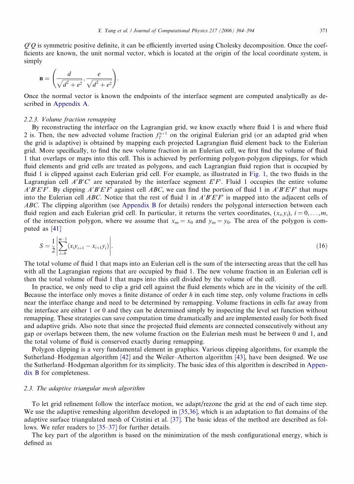
QtQ is symmetric positive definite, it can be efficiently inverted using Cholesky decomposition. Once the coef-ficients are known, the unit normal vector, which is located at the origin of the local coordinate system, issimply

n ¼ dffiffiffiffiffiffiffiffiffiffiffiffiffiffiffid2 þ e2

p ;effiffiffiffiffiffiffiffiffiffiffiffiffiffiffi

d2 þ e2p

!.

Once the normal vector is known the endpoints of the interface segment are computed analytically as de-scribed in Appendix A.

2.2.3. Volume fraction remapping

By reconstructing the interface on the Lagrangian grid, we know exactly where fluid 1 is and where fluid2 is. Then, the new advected volume fraction f nþ1

T on the original Eulerian grid (or an adapted grid whenthe grid is adaptive) is obtained by mapping each projected Lagrangian fluid element back to the Euleriangrid. More specifically, to find the new volume fraction in an Eulerian cell, we first find the volume of fluid1 that overlaps or maps into this cell. This is achieved by performing polygon-polygon clippings, for whichfluid elements and grid cells are treated as polygons, and each Lagrangian fluid region that is occupied byfluid 1 is clipped against each Eulerian grid cell. For example, as illustrated in Fig. 1, the two fluids in theLagrangian cell A 0B 0C 0 are separated by the interface segment E 0F 0. Fluid 1 occupies the entire volumeA 0B 0E 0F 0. By clipping A 0B 0E 0F 0 against cell ABC, we can find the portion of fluid 1 in A 0B 0E 0F 0 that mapsinto the Eulerian cell ABC. Notice that the rest of fluid 1 in A 0B 0E 0F 0 is mapped into the adjacent cells ofABC. The clipping algorithm (see Appendix B for details) renders the polygonal intersection between eachfluid region and each Eulerian grid cell. In particular, it returns the vertex coordinates, (xi,yi), i = 0, . . . ,m,of the intersection polygon, where we assume that xm = x0 and ym = y0. The area of the polygon is com-puted as [41]

S ¼ 1

2

Xm�1

i¼0

ðxiyiþ1 � xiþ1yiÞ��

��. ð16Þ

The total volume of fluid 1 that maps into an Eulerian cell is the sum of the intersecting areas that the cell haswith all the Lagrangian regions that are occupied by fluid 1. The new volume fraction in an Eulerian cell isthen the total volume of fluid 1 that maps into this cell divided by the volume of the cell.

In practice, we only need to clip a grid cell against the fluid elements which are in the vicinity of the cell.Because the interface only moves a finite distance of order h in each time step, only volume fractions in cellsnear the interface change and need to be determined by remapping. Volume fractions in cells far away fromthe interface are either 1 or 0 and they can be determined simply by inspecting the level set function withoutremapping. These strategies can save computation time dramatically and are implemented easily for both fixedand adaptive grids. Also note that since the projected fluid elements are connected consecutively without anygap or overlaps between them, the new volume fraction on the Eulerian mesh must be between 0 and 1, andthe total volume of fluid is conserved exactly during remapping.

Polygon clipping is a very fundamental element in graphics. Various clipping algorithms, for example theSutherland–Hodgeman algorithm [42] and the Weiler–Atherton algorithm [43], have been designed. We usethe Sutherland–Hodgeman algorithm for its simplicity. The basic idea of this algorithm is described in Appen-dix B for completeness.

2.3. The adaptive triangular mesh algorithm

To let grid refinement follow the interface motion, we adapt/rezone the grid at the end of each time step.We use the adaptive remeshing algorithm developed in [35,36], which is an adaptation to flat domains of theadaptive surface triangulated mesh of Cristini et al. [37]. The basic ideas of the method are described as fol-lows. We refer readers to [35–37] for further details.

The key part of the algorithm is based on the minimization of the mesh configurational energy, which isdefined as


E ¼ 1

2

Xedges

c2; ð17Þ

where the edge tensions are c = l � l0, l is the local edge length, and l0 is an optimal edge length. The optimaledge length is determined from the relevant local length scale of a specific problem, for example, the distanceof a local point to the nearest interface, the radius of curvature, and the distance between two interfaces. Themesh energy is an integral measure of how local edge lengths deviate from an optimal value. Minimization ofthe mesh energy (17) implies that l � l0, i.e., the optimal mesh is achieved by the minimization of mesh energy.

By defining the mesh energy (17), the mesh is analogous to a system of springs. For a fixed mesh topology,the minimization of the mesh energy (17) is thus equivalent to the relaxation of a dynamical system of masslesssprings with tensions c and damping coefficients of unity. Accordingly, the position x of a node evolves with avelocity _x proportional to the vector sum of spring forces acting on the node. Therefore,

_x ¼XNc

j¼1

ejcj; ð18Þ

where Nc is the coordination number of the node, and ej is the unit vector parallel to edge j.Node displacements reduce the mesh energy and lead to equilibrium of tensions at all nodes. However, due

to topological constraints the tensions themselves are in general nonzero. To further reduce the mesh energy, itis necessary to perform topological mesh restructuring operations, which include node addition, subtraction,and reconnection. Node addition/subtraction is needed when grids need to be refined/coarsened in some localregion. Node reconnection is used to reconnect some of the nodes such that the elements formed by thesenodes become more regular, or not extremely stretched. For specific details, see [35–37]. Topological restruc-turing operations provide access to mesh configurations with lower energy than accessible by mesh relaxation.The relaxation and topological restructuring are performed iteratively until j _xj is less than a prescribed valueand the criteria for node addition, subtraction and reconnection are no longer satisfied.

The resulting mesh maintains the resolution of the relevant local length scale everywhere with prescribedaccuracy. The minimization depends only on the instantaneous configuration of the interface, and is insensi-tive to the deformation history.

2.4. The Stokes flow solver

To simulate a real problem, for example drop deformation in an extensional flow, we coupled our interfacecapturing method with a finite element based Stokes flow solver. The governing equations for the flow solverare

�r � ðlðruþ ðruÞtÞÞ þ rp ¼ r � F s; ð19Þr � u ¼ 0; ð20Þ

with Dirichlet (for prescribed boundary flows, e.g., shear and no-slip flows) and/or Neumann-type (free-slip)boundary conditions (see [36]), where l is the dynamic viscosity of the local fluid, p is the pressure,Fs = rdR(I � n � n) is the capillary pressure tensor, r is the surface tension coefficient, dR = d(/)j$/j is thesurface delta function, and I is the identity matrix. The local dynamic viscosity l is equal to l1 in fluid 1,l2 in fluid 2. Notice that since we use the continuum surface stress formulation, the curvature of the interfacedoes not explicitly appear in Eq. (19).

The Stokes equations are solved using the Mini finite element method [44]. The finite element spaces are

V h ¼ fv 2 ðH 1ðXÞÞ2 : vjT 2 ðP 1ðT ÞÞ2; 8T 2Th; vjoXD¼ 0; v � �njoXN

¼ 0g� fv : vjT 2 ðP 3ðT ÞÞ2 \ ðH 1

0ðT ÞÞ2; 8T 2Thg; ð21Þ

Qh ¼ q 2 C0ðXÞ \ L2ðXÞ : qjT 2 P 1ðT Þ; 8T 2Th;

ZX

q ¼ 0

� �ð22Þ

for velocity and pressure, respectively, where oXD denotes Dirichlet boundary, oXN denotes Neumann-typeboundary, and �n is the normal to oXN.


Multiplying Eq. (19) by vh 2 Vh and Eq. (20) by qh 2 Qh, we get the weak formulation for the unknowns(uh,ph) 2 Vh · Qh:
Z
Xlðruh þ ðruhÞtÞ : rvh �

ZX

phr � vh ¼ �Z

XF s : rvh; ð23ÞZ

Xqhr � uh ¼ 0 ð24Þ

for all test functions (vh,qh) 2 Vh · Qh. See [36] for a derivation.To evaluate the surface stress in the above weak formulation, the normal vector n at a cell vertex is calcu-

lated from the continuous level set function using a least squares fit similar to that described in Section 2.2.2.The only differences are that the origin of the local coordinate system is located at the cell vertex, and thefitting is over a stencil that consists of the vertex under consideration and all its nearest neighbors. In addition,as is in [36], in practice the Dirac delta function d(/) is replaced by a smoothed version d�(/), where d�(/) =dH�/d/ and H� is a smoothed Heaviside function, defined as

H �ð/Þ ¼0 if / < ��;12

1þ /�þ 1

p sin p/�

� �� if j/j 6 �;

1 if / > �;

8><>: ð25Þ

where the parameter � is taken to be 2–4 times the smallest mesh size. The local dynamic viscosity l is alsosmoothed using the smoothed Heaviside function. Thus,

l ¼ l1 þ ðl2 � l1ÞH �ð/Þ. ð26Þ
The resulting linear system from the discretization is solved using an inexact Uzawa method [45]. Matrix inver-sions are performed using SSOR preconditioned conjugate gradient method. See also [36].
2.5. Summary

The whole procedure is summarized as follows:

(1) At the beginning of a computation, the initial values of /, and f are specified according to the initialinterface position. Then, the flow field, i.e. the velocity and pressure, are initialized by solving the Stokesequations. Notice that since the Stokes equations are time independent, they can be solved as a quasi-steady problem at any time instance.

(2) Knowing the initial values of /, f and u, or the values of /, f and u at time level n, we perform (i) the firststep of the two-stage RKDG Eulerian level set evolution to obtain the intermediate Eulerian level setfunction, /n+1/2, on the Eulerian grid; and (ii) the first step of the two-stage Runge–Kutta projectionof the grid, in which grid nodes are projected according to Eq. (12). The projection results in an inter-mediate Lagrangian mesh. The position of a node in the intermediate Lagrangian mesh is given by~x

nþ1=2i .

(3) The intermediate Eulerian velocity uðxni ; t

nþ12Þ is obtained by solving the Stokes equations on the Eulerian

mesh, for which the interface normal vector in the surface stress term is calculated from the intermediatelevel set function /n+1/2. The intermediate Lagrangian velocity uð~xnþ1=2

i ; tnþ12Þ is obtained from the inter-

mediate Eulerian velocity uðxni ; t

nþ12Þ through interpolation.

(4) Then, the second step of the RKDG level set evolution is performed to solve for /n+1, the Eulerian levelset function at time level n + 1, and the second step of the Runge–Kutta grid projection is performed toobtain the final Lagrangian mesh corresponding to time level n + 1, in which grid nodes are projectedaccording to Eq. (13).

(5) The volume fractions remain the same during the projection according to Eq. (10). The level set functionon the final Lagrangian grid is obtained from /n+1 through interpolation. Based on both the level setfunction and volume fraction, we reconstruct an interface on the final Lagrangian grid, as describedin Section 2.2.2.


(6) To let grid refinement follow the interface motion, grid is adapted/rezoned based on the current interfaceposition, which results in a new Eulerian grid.

(7) The values of f on the new Eulerian grid are obtained through remapping, as described in Section 2.2.3.The level set function on the new Eulerian grid is directly obtained as the signed distance function to thepreviously reconstructed interface on the Lagrangian grid. The distance function is calculated as the min-imum distance of a point to the linear segments that constitute the interface. The flow velocity on thenew Eulerian grid is obtained by solving the Stokes equations.

(8) Steps 2–7 are repeated until a specified end time is reached.

3. Results

In this section, we examine the integrity and accuracy of our ACLSVOF interface reconstruction and vol-ume tracking method, and present numerical simulations of drop deformation in an extensional flow using ouradaptive ACLSVOF method, for which the flow velocity is solved using the Stokes flow solver described inSection 2.4.

3.1. Interface reconstruction test

3.1.1. Reconstruction of a linear interfaceFor a linear interface defined by n Æ x = a, the analytic level set function is given by / = n Æ x � a, which is a

linear function of the coordinates of a point. Because the least squares quadratic fitting approximates a linearfunction exactly, our normal calculation method, described in Section 2.2.2, computes the normal vector of alinear interface exactly. In addition, because the linear interface segments are finally reconstructed analyticallyusing the analytic reconstruction method, described in Appendix A, our interface reconstruction methodreconstructs a linear interface exactly. This implies that our interface reconstruction method is second orderaccurate [46].

3.1.2. Reconstruction of a circular interface

A circle of radius 0.368 centered at (0.525,0.464) in a (0,1) · (0, 1) computational domain is reconstructedusing the CLSVOF interface reconstruction method described in Section 2.2.2. The discrete volume fractiondata are initialized exactly as the volume ratio of each cell occupied by the interior fluid. The level set at eachnode point is initialized exactly as the signed minimum distance of the node to the circle.

Fig. 3 shows the reconstructed interface on a 2 · 102 uniform triangular grid, which is obtained from a 102

uniform rectangular grid by dividing each rectangular cell into two triangular cells along one of its diagonals.The difference between the reconstructed interface and the analytic interface is nearly invisible.

To quantify the reconstruction error, an L1 error norm is defined. Since a reconstructed interface segmentdoes not exactly coincide with the analytic interface, there is a volume mismatch between the analytic interfaceand the reconstructed interface, as illustrated in Fig. 4. The L1 error norm is defined as the summation of thevolume mismatches in all interfacial cells, and is computed analytically. Table 1 shows the reconstructionerrors and convergence rates on five uniform triangular grids. The results verify that our interface reconstruc-tion method is second order accurate.

3.2. Volume tracking tests

Uniform translation and solid body rotation tests have been used widely for assessing the integrity and capa-bility of an interface tracking method [6]. As stated in [6], ‘‘an acceptable volume tracking method must trans-late and rotate fluid bodies without significant distortion or degradation of fluid interfaces. Mass should also beconverged rigorously in these cases’’. However, simple translation and rotation tests provide only a minimalassessment of the capability of a volume tracking method since the interface does not deform. Interfacial flows,for example the Rayleigh–Taylor, Richtmeyer–Meshkov, and Kelvin–Helmholtz instabilities, often involvestrong vortical flows near the interface, and thus complex changes of the interface. ‘‘A complete assessment

Fig. 4. Volume mismatch (shaded area) between the analytic circle and the reconstructed linear interface in a triangular cell.

Table 1L1 error norms, and convergence rates for circle reconstruction

Triangles L1 error Order

2 · 102 1.47E�3 –2 · 202 3.17E�4 2.212 · 402 8.67E�5 1.872 · 802 1.94E�5 2.162 · 1602 5.26E�6 1.88

0 0.2 0.4 0.6 0.8 10

0.2

0.4

0.6

0.8

1

x

y

Fig. 3. Reconstructed interface on a 2 · 102 uniform triangular grid. The difference between the reconstructed interface and the analyticinterface, which is plotted using a dotted line, is nearly invisible.


of interface tracking methods should therefore impose strong vorticity at the interface’’ [15]. We refer readers tothe articles by Rider and Kothe [6,15] for an elegant discussion of choosing appropriate test problems.

In this section, we present results for four selected test problems: simple translation, and rotation of a cir-cular fluid body, solid body rotation of Zalesak’s slotted disk [47], and the single vortex problem introducedby Rider and Kothe [15], where the single vortex problem provides a rigorous test of a volume trackingmethod in cases where significant interface stretching occurs. These test problems have been widely usedrecently [6,23,24,30,48].

For the solid body rotation of Zalesak’s slotted disk, the geometry and grid were chosen to allow comparisonto data in the literature and are described below in Section 3.2.3. For all other tests, we perform convergencestudies, for which an L1 error norm is defined as


EL1 ¼Z

Xjf computedðx; tÞ � f exactðx; tÞjdx. ð27Þ

Convergence studies are performed on both fixed uniform grids and adaptive clustered grids. The fixed uni-form grids are obtained from the corresponding uniform structured rectangular grids, with edge lengths of0.032, 0.016, and 0.008, respectively, by dividing each rectangular cell into two triangular cells. For all adap-tive grids, grids are clustered near the interface to render high resolution near the interface. The edge lengths ofthe smallest grid cells, denoted by hmin, are roughly 0.032, 0.016, and 0.008, respectively for the three sets ofadaptive grids. We expect the errors on the adaptive grids to be about the same size as on the correspondinguniform grids, because only the grid in the vicinity of the interface should affect the accuracy of the evolutionof the interface position, but many fewer grid cells are used on the adaptive grids than on corresponding uni-form grids. The CFL number for these tests is 0.7. The computational domain is a (0, 1) · (0, 1) square.

To quantify the accuracy of mass conservation of the method, we define a time averaged mass error as

EM ¼Z T f

t¼0

jMðtÞ �Mð0ÞjT f

dt; ð28Þ

where

MðtÞ ¼Z

Xf ðx; tÞdx ð29Þ

and Tf is the total integration time. As the velocity fields are given analytically for these tests, volume changesin these tests are primarily due to reasons (ii), (iii) and (iv), as elaborated in Section 2.2.1.

3.2.1. Simple translation of a circular fluid body

An initially circular fluid body of radius 0.25 centered in the computational domain is translated by a uni-form velocity field along the 45� domain diagonal. The velocity remains constant with unit components, butchanges sign at times 0.25 and 0.75, respectively. Therefore, the fluid body should return to its initial positionafter 1 time unit without any interface deformation.

Fig. 5 shows the final reconstructed interfaces and the corresponding L1 error contours on the three sets ofadaptive grids. The reconstructed interface and error contours are isotropic with respect to flow, exhibiting nobias towards the flow direction. The total number of triangles is subject to change as the grid adapts to theevolving interface. At t = 0, the total numbers of triangles in the computational domain are 764, 1722, and3590, respectively, which are much less than the number of triangles of the corresponding uniform grids, espe-cially as the minimum grid sizes become smaller (see Table 2).

Table 2 shows that our volume tracking method translates a fluid body with second order accuracy on bothuniform grids and adaptive clustered grids. In addition, as we have expected, the L1 errors on the adaptivegrids are very close to those on the corresponding uniform grids because they have similar minimum grid sizes,while using significantly fewer grid cells. It is also shown that the mass errors are zero on each of the grids,verifying that our method conserves mass exactly for simple translation problems because the second orderRunge–Kutta method integrates a constant function exactly.

3.2.2. Solid body rotation of a circular fluid body

An initially circular fluid body of radius 0.15 centered at the point (0.5,0.75) is revolved around the centerof the unit domain with a constant unit angular velocity for one complete revolution. Therefore, the fluid bodyshould return to its initial position after 2p time units without any change in the interface shape.

Fig. 6 shows the final reconstructed interface and the corresponding L1 error contours on the three sets ofadaptive grids. Table 3 shows second order convergence in the L1 error norms for both uniform grids andadaptive grids. Again, the L1 errors on the adaptive grids are very close to those on the corresponding uniformgrids having similar minimum grid sizes, while the number of triangles are greatly reduced by using adaptivegrids. The time averaged mass errors are not zero because the projection of a fluid element subject to rotationcan not be integrated exactly. However, the mass errors are very small compared to the total mass of the drop,

0 0.1 0.2 0.3 0.4 0.5 0.6 0.7 0.8 0.9 10

0.1

0.2

0.3

0.4

0.5

0.6

0.7

0.8

0.9

1

x

y

x

y

0 0.1 0.2 0.3 0.4 0.5 0.6 0.7 0.8 0.9 10

0.1

0.2

0.3

0.4

0.5

0.6

0.7

0.8

0.9

1

0 0.1 0.2 0.3 0.4 0.5 0.6 0.7 0.8 0.9 10

0.1

0.2

0.3

0.4

0.5

0.6

0.7

0.8

0.9

1

x

y

x

y

0 0.1 0.2 0.3 0.4 0.5 0.6 0.7 0.8 0.9 10

0.1

0.2

0.3

0.4

0.5

0.6

0.7

0.8

0.9

1

0 0.1 0.2 0.3 0.4 0.5 0.6 0.7 0.8 0.9 10

0.1

0.2

0.3

0.4

0.5

0.6

0.7

0.8

0.9

1

x

y

x

y

0 0.1 0.2 0.3 0.4 0.5 0.6 0.7 0.8 0.9 10

0.1

0.2

0.3

0.4

0.5

0.6

0.7

0.8

0.9

1

a b

c d

e f

Fig. 5. Reconstructed interfaces (left) and the corresponding L1 error contours (right) of an initially circular fluid body after a completediagonal translation. hmin � 0.032, 0.016, and 0.008, respectively from top to the bottom. The contours are of 20 levels from �3.1 · 10�6 to2.7 · 10�6 for (b), from �4.0 · 10�7 to 2.9 · 10�7 for (d), and from �9.2 · 10�8 to 7.2 · 10�8 for (f).


Table 2L1 error norms, convergence rates and time averaged mass errors for the simple translation test

hmin Triangles L1 error Order Mass error

Fixed uniform grids

0.032 2048 7.10E�5 – 0.00.016 8192 1.67E�5 2.09 0.00.008 32768 3.61E�6 2.21 0.0

Adaptive grids

0.032 764 9.14E�5 – 0.00.016 1722 1.80E�5 2.34 0.00.008 3590 5.07E�6 1.83 0.0


and because they are much lower than the L1 error norms, the mass errors do not nullify our convergencestudy. In addition, it is seen that the mass errors are significantly reduced by refining the grid.

3.2.3. Zalesak slotted disk rotation

Zalesak slotted disk [47] (refer to Fig. 7) is revolved about the center of the computational domain with aconstant angular velocity. To compare our results with other’s, we consider Rudman’s version [49] of thisproblem, in which the specifications of the geometry are slightly modified from [47]. In particular, the com-putational domain is a (0, 4) · (0,4) square. The circle is centered at (2,2.75), with a diameter of 1. The widthof the slot is 0.12. The maximum width of the upper bridge, that connects the left and right portions of thecircle, is 0.4. The constant angular velocity is 0.5. Thus, the disk should return to its initial position after4p time units without any interface change.

In most previous works, uniform rectangular grids, with 200 cells along each coordinate direction, wereused. To compare our results to these previous works, we present test results on both a fixed uniform trian-gular grid and adaptive triangular grids. The uniform triangular grid is obtained from the uniform rectangulargrid, with 200 cells along each coordinate direction, by dividing each rectangular cell into two triangles alongone of its diagonals. For adaptive grids, we refine the grid near the interface such that the edge length of thesmallest cells is roughly 0.02. In addition, as in [49] the time step is chosen such that a complete revolution iscompleted in 2524 time steps, corresponding to a Courant number of about 0.25, and the errors for this testare computed as

EZ ¼P

T jfcomputedT � f exact

T jPT f exact

T

. ð30Þ

Fig. 7(a) shows the reconstructed slotted disk after one complete revolution on an adaptive grid. The differencebetween the reconstructed disk and the exact solution is only visible in the small regions near the sharp cor-ners, where the sharp corners are smoothed due to the linear reconstruction of the interface. This is consistentwith those results presented by other researchers, for example in [49,48,23]. However, our result looks moresymmetric than most other similar results, and is comparable with the results obtained using quadratic inter-face reconstruction methods in [23] (refer to Fig. 8 in [23] for a comparison). This is more evident when look-ing at the results after 10 complete revolutions, shown in Fig. 7(b) (refer to Fig. 9 in [23] for a comparison). Itis seen that even after 10 complete revolutions most of the reconstructed interface still coincides with the exactsolution. There is only mild overshooting at the corners. The adaptive grid for this computation is shown inFig. 7(c), which only uses about 5500 grid cells, compared to 2 · 200 · 200 grid cells on the uniform grid.Fig. 7(d) shows the reconstructed slotted disk after 10 complete revolutions on a refined adaptive grid, theminimum grid size of which is

ffiffiffi2p

times smaller than that of the previous grid. We see that refining the griddoes improve the accuracy.

The EZ errors after one complete revolution are tabulated in Table 4, and are compared with the errorspresented by other researchers. It is seen that the error on the fixed uniform triangular grid is smaller thanmost of the other errors, and is only bigger than the errors of Scardovelli and Zaleski obtained using aquadratic fit. The error on adaptive grid is slightly larger than the error on the uniform triangular grid. Thisdifference is mainly because the control of the smallest grid size of the adaptive grid is only approximate, i.e.,

0 0.1 0.2 0.3 0.4 0.5 0.6 0.7 0.8 0.9 10

0.1

0.2

0.3

0.4

0.5

0.6

0.7

0.8

0.9

1

x

y

x

y

0 0.1 0.2 0.3 0.4 0.5 0.6 0.7 0.8 0.9 10

0.1

0.2

0.3

0.4

0.5

0.6

0.7

0.8

0.9

1

0 0.1 0.2 0.3 0.4 0.5 0.6 0.7 0.8 0.9 10

0.1

0.2

0.3

0.4

0.5

0.6

0.7

0.8

0.9

1

x

y

x

y

0 0.1 0.2 0.3 0.4 0.5 0.6 0.7 0.8 0.9 10

0.1

0.2

0.3

0.4

0.5

0.6

0.7

0.8

0.9

1

0 0.1 0.2 0.3 0.4 0.5 0.6 0.7 0.8 0.9 10

0.1

0.2

0.3

0.4

0.5

0.6

0.7

0.8

0.9

1

x

y

x

y

0 0.1 0.2 0.3 0.4 0.5 0.6 0.7 0.8 0.9 10

0.1

0.2

0.3

0.4

0.5

0.6

0.7

0.8

0.9

1

a b

c d

e f

Fig. 6. Reconstructed interfaces (left) and the corresponding L1 error contours (right) of an initially circular fluid body after a completerevolution. hmin � 0.032, 0.016, and 0.008, respectively from top to the bottom. The contours are of 20 levels from �1.9 · 10�5 to1.9 · 10�5 for (b), from �2.6 · 10�6 to 2.1 · 10�6 for (d), and from �3.0 · 10�7 to 4.0 · 10�7 for (f).


Table 3L1 error norms, convergence rates and time averaged mass errors for the solid body rotation test

hmin Triangles L1 error Order Mass error

Fixed uniform grids

0.032 2048 5.61E�4 – 2.59E�70.016 8192 1.28E�4 2.13 3.75E�80.008 32768 3.48E�5 1.88 4.57E�9

Adaptive grids

0.032 523 4.09E�4 – 1.20E�60.016 1107 1.01E�4 2.02 2.45E�70.008 2246 2.54E�5 1.99 2.16E�8

1.4 1.6 1.8 2 2.2 2.4 2.6

2.2

2.4

2.6

2.8

3

3.2

x

y

1.4 1.6 1.8 2 2.2 2.4 2.6

2.2

2.4

2.6

2.8

3

3.2

x

y

1.4 1.6 1.8 2 2.2 2.4 2.6

2.2

2.4

2.6

2.8

3

3.2

x

y

1.4 1.6 1.8 2 2.2 2.4 2.6

2.2

2.4

2.6

2.8

3

3.2

x

y

a b

c d

Fig. 7. Zalesak slotted disk test. (a) The reconstructed disk (solid line) and the exact solution (dotted line) after one complete revolution.hmin � 0.02. (b) The reconstructed disk (solid line) and the exact solution (dotted line) after 10 complete revolutions. hmin � 0.02. (c) Thereconstructed disk and the computational grid after 10 complete revolutions. hmin � 0.02. (d) The reconstructed disk (solid line) and theexact solution (dotted line) after 10 complete revolutions. hmin � 0.014.


Table 4EZ errors for Zalesak slotted disk test after one complete revolution

Advection/reconstruction methods EZ error

SLIC 8.38E�2Hirt–Nichols 9.62E�2FCT–VOF 3.29E�2Youngs 1.09E�2Harvie and Fletcher (Stream/Youngs) 1.07E�2Harvie and Fletcher (Stream/Puckett) 1.00E�2Lopez et al. (EMFPA-SIR) 8.74E�3present ACLSVOF (uniform triangular grid) 7.19E�3present ACLSVOF (adaptive triangular grid) 1.25E�2Scardovelli and Zaleski (linear least-square fit) 9.42E�3Scardovelli and Zaleski (quadratic fit) 5.47E�3Scardovelli and Zaleski (quadratic fit + continuity) 4.16E�3

All previous results are taken from Table 3 in [48].


the smallest grid cells vary slightly in size spatially and temporally. The time averaged mass errors for this testare on the order of 10�9, which is extremely small.

3.2.4. Single vortex flow

An initially circular fluid body of radius 0.15 centered at the point (0.5,0.75) is evolved by a single vortexflow field. The flow field is given by the stream function

W ¼ 1

psin2ðpxÞ sin2ðpyÞ; ð31Þ

where the velocity vector is defined by (�oW/oy,oW/ox). This flow field was first introduced by Bell et al. in[50], and first used as the flow field in the ‘‘single vortex’’ problem for assessing the integrity and capability ofan interface tracking method by Rider and Kothe in [15]. The flow field contains a single vortex centered in thedomain. The vortex spins fluid elements, stretching them into a thin filament that spirals toward the vortexcenter. Thus each fluid element can undergo very large deformation.

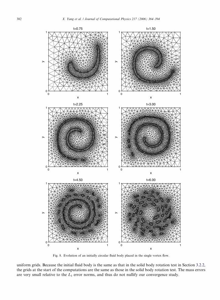
Fig. 8 shows the evolution of the circular fluid body in the single vortex flow field. The solution is computedusing an adaptive mesh of moderate resolution, for which the smallest grid cell has an edge length of 0.016. Itis seen that the fluid body is spun into a thinning filament, which compares very well with those resultsobtained using other state-of-the-art methods, for example [6,24]. Theoretically, the filament spirals towardthe vortex center, and becomes thinner and thinner continuously. However, Fig. 8 shows that the thin filamentbreaks into small pieces beginning at its tail after long time evolution. This is because the grid resolution hasbecome low relative to the thinning filament when the thickness of the filament is equal to or less than the gridsize. Because the interface is represented by a single line segment in each interfacial grid cell, any two interfacesmerge automatically whenever they come into the same cell, resulting in an unphysical ‘pinch-off’. Once thepinch-off occurs, the linear segment approximation of an interface immediately flattens the high curvatureregion, effectively applying numerical surface tension. Because the filament asymptotes to infinitesimal thick-ness, any grid will eventually provide inadequate resolution. However, this unphysical pinch-off can be delayedby refining the grid near the interface. Because we have implemented adaptive unstructured grids in our algo-rithm, we can refine the grid near the interface efficiently.

For convergence studies, the Leveque cosine term [51] is applied to the velocity field, i.e., the flow fielddefined by (31) is multiplied by cos(pt/Tf). By doing this, the flow field reverses in time such that any fluid bodyreturns to its initial position at time Tf, allowing the error to be quantified with Eq. (27). Convergence studiesare performed for three different values of Tf on both fixed uniform grids and adaptive grids. Fig. 9 shows thereconstructed interfaces and the corresponding L1 error contours on the adaptive grid of hmin � 0.016 for thethree values of Tf. Quantitative error measurements and convergence rates are shown in Table 5. The conver-gence rates show that our ACLSVOF method is second order accurate, even when Tf is large, for which largecomplex topological change has occurred (see Fig. 10), indicating that our method is remarkably resilient forinterface capturing. Once again, we see that the errors on the adaptive grids are similar to those on fixed

0 10

1t=0.75

x

y

0 10

1t=1.50

x

y

0 10

1t=2.25

x

y

0 10

1t=3.00

x

y

0 10

1t=4.50

x

y

0 10

1t=6.00

x

y

Fig. 8. Evolution of an initially circular fluid body placed in the single vortex flow.


uniform grids. Because the initial fluid body is the same as that in the solid body rotation test in Section 3.2.2,the grids at the start of the computations are the same as those in the solid body rotation test. The mass errorsare very small relative to the L1 error norms, and thus do not nullify our convergence study.

0 0.1 0.2 0.3 0.4 0.5 0.6 0.7 0.8 0.9 10

0.1

0.2

0.3

0.4

0.5

0.6

0.7

0.8

0.9

1

x

yy

x

y

0 0.1 0.2 0.3 0.4 0.5 0.6 0.7 0.8 0.9 10

0.1

0.2

0.3

0.4

0.5

0.6

0.7

0.8

0.9

1

0 0.1 0.2 0.3 0.4 0.5 0.6 0.7 0.8 0.9 10

0.1

0.2

0.3

0.4

0.5

0.6

0.7

0.8

0.9

1

x x

y

0 0.1 0.2 0.3 0.4 0.5 0.6 0.7 0.8 0.9 10

0.1

0.2

0.3

0.4

0.5

0.6

0.7

0.8

0.9

1

0 0.1 0.2 0.3 0.4 0.5 0.6 0.7 0.8 0.9 10

0.1

0.2

0.3

0.4

0.5

0.6

0.7

0.8

0.9

1

x

y

x

y

0 0.1 0.2 0.3 0.4 0.5 0.6 0.7 0.8 0.9 10

0.1

0.2

0.3

0.4

0.5

0.6

0.7

0.8

0.9

1

a b

c d

e f

Fig. 9. Reconstructed interfaces (left) and the corresponding L1 error contours (right) for an initially circular fluid body placed in a time-reversed, single vortex flow on an adaptive grid of hmin � 0.016 at t = Tf, where Tf = 0.5, 2.0 and 8.0, respectively from top to the bottom.The contours are of 20 levels from �5.9 · 10�7 to 6.9 · 10�7 for (b), from �2.0 · 10�5 to 1.3 · 10�5 for (d), and from �9.2 · 10�5 to8.8 · 10�5 for (f).


Table 5L1 error norms, convergence rates and time averaged mass errors for the time-reversed, single vortex test

Tf hmin Fixed uniform grids Adaptive grids

L1 error order Mass error L1 error order Mass error

0.5 0.032 1.26E�4 – 7.64E�6 1.97E�4 – 1.86E�50.016 2.41E�5 2.39 3.17E�6 2.58E�5 2.93 3.01E�60.008 4.30E�6 2.49 3.09E�7 5.24E�6 2.30 2.76E�7

2.0 0.032 1.41E�3 – 2.53E�5 1.62E�3 – 3.40E�50.016 3.38E�4 2.06 5.25E�6 3.36E�4 2.27 6.45E�60.008 6.84E�5 2.30 4.86E�7 7.95E�5 2.08 3.79E�7

8.0 0.032 3.70E�2 – 7.01E�5 3.54E�2 – 7.57E�50.016 3.75E�3 3.30 7.66E�6 3.56E�3 3.31 1.41E�50.008 5.61E�4 2.74 1.45E�6 5.09E�4 2.81 1.30E�6

0 0.1 0.2 0.3 0.4 0.5 0.6 0.7 0.8 0.9 10

0.1

0.2

0.3

0.4

0.5

0.6

0.7

0.8

0.9

1

x

y

Fig. 10. Reconstructed interface of an initially circular fluid body placed in a time-reversed, single vortex flow on an adaptive grid ofhmin � 0.016 at t = Tf/2, for Tf = 8.0.


In Tables 6 and 7, we compare our results with those presented by other researchers. We point out that allthe results presented by other researchers were obtained using uniform structured rectangular grids. Ourresults were obtained on both fixed uniform triangular grids and adaptive triangular grids. For comparison,the minimum grid sizes of our grids were controlled to be similar to the grid sizes of the corresponding rect-angular grids. Table 6 shows the L1 error norms, and convergence rates obtained using different methods forTf = 2.0. It is seen that all of the methods are about second order accurate, and the error levels of the methodsare fairly close to each other. Table 7 shows the L1 error norms obtained using different methods for Tf = 8.0.All previous results were obtained on a 128 · 128 rectangular grid. Results of the present paper were obtainedon a fixed uniform grid and an adaptive grid (both with hmin � 0.008), respectively. It is seen that the errors ofour method are among the lowest ones, except that of Aulisa et al. [52] obtained using a marker and local areaconservation method, which is much lower than all of the other errors.

3.3. Simulation of drop deformation in an extensional flow

In this section, we simulate a physical problem by coupling our adaptive CLSVOF interface capturingmethod with a Stokes flow solver, that is, the interface will be captured using our adaptive CLSVOF methods

Table 6L1 error norms, and convergence rates obtained using different methods for the time-reversed, single vortex test with Tf = 2.0

Computational methods Grid size L1 error Order

Garrioch and Baliga (Pilliod–Puckett advection circle fit) 32 · 32 2.23E�3 –64 · 64 4.93E�4 2.18128 · 128 1.12E�4 2.14

Scardovelli and Zaleski (linear fit) 32 · 32 1.75E�3 –64 · 64 4.66E�4 1.91128 · 128 1.02E�4 2.19

Scardovelli and Zaleski (quadratic fit) 32 · 32 1.88E�3 –64 · 64 4.42E�4 2.08128 · 128 9.36E�5 2.24

Scardovelli and Zaleski (quadratic fit + continuity) 32 · 32 1.09E�3 –64 · 64 2.80E�4 1.96128 · 128 5.72E�5 2.29

Aulisa et al. (markers/VOF) 32 · 32 1.00E�3 –64 · 64 2.69E�4 1.89128 · 128 5.47E�5 2.30

Lopez et al. (EMFPA-SIR) 32 · 32 8.62E�4 –64 · 64 2.37E�4 1.86128 · 128 5.62E�5 2.08

Present (fixed uniform grids) hmin = 0.032 1.41E�3 –hmin = 0.016 3.38E�4 2.06hmin = 0.008 6.84E�5 2.30

Present (adaptive grids) hmin � 0.032 1.62E�3 –hmin � 0.016 3.36E�4 2.27hmin � 0.008 7.95E�5 2.08

All previous results are taken from Table 5 in [48].

Table 7L1 error norms obtained using different methods for the time-reversed, single vortex test with Tf = 8.0

Advection/reconstruction methods L1 error

Rider and Kothe/Puckett 1.44E�3Harvie and Fletcher/Youngs 2.16E�3Harvie and Fletcher/Puckett 1.18E�3EMFPA/Youngs 2.13E�3EMFPA/Puckett 1.17E�3EMFPA-SIR 7.57E�4Aulisa et al., markers/VOF 4.78E�4Aulisa et al., markers/local area conservation 4.06E�5Present (fixed uniform grids) 5.61E�4Present (adaptive grids) 5.09E�4

All previous results were taken from Table 7 in [48], except that the result of Aulisa et al. (markers/local area conservation) was taken fromTable 1 in [52]. All previous results were obtained on a 128 · 128 rectangular grid. Results of the present paper were obtained on a fixeduniform grid and an adaptive grid (both with hmin � 0.008), respectively.


and the velocity field will be computed by the Stokes flow solver. More specifically, we consider drop defor-mation in an extensional flow, which is modeled by experimentalists in four-roll mill devices, first introducedby G.I. Taylor [53]. A schematic of the problem is shown in Fig. 11.

The control of drop deformation and breakup is of fundamental importance in numerous industrial appli-cations such as the dispersion of immiscible fluids into each other to create emulsions, the separation of liquidphases by tip streaming, and so on. It has attained wide investigation in the past and is still under intensiveresearch [53–56]. A milestone, since the pioneering work by Taylor [53], is the experimental work by Bentley

Fig. 11. Schematic of drop deformation in an extensional flow.


and Leal [54]. They designed a computer-controlled four-roll mill apparatus, which enabled them automatic,flexible and accurate control of the experiment with the capability to investigate drop deformation andbreakup in a wide range of flow conditions, in particular, the transient flow in between pure extensional flowand pure shear flow, which had not been investigated experimentally up to then. Their work not only providedthe first experimental data for drop deformation and breakup in this transient flow, but also improved the datafor drop deformation in pure extensional flow and pure shear flow. The validity of small deformation theoryand slender drop theory was also clarified. For a review of the research prior to 1994, we refer readers to thereview paper by Stone [57].

We limit our simulation to two-dimensional low-speed Newtonian viscous flow with clean interfaces.Two dimensionless parameters determine the behavior of such a flow: the capillary number Ca and the vis-cosity ratio k, where Ca = lGa/r, l is the viscosity of the suspending fluid, G is the applied strain rate, a isthe radius of the undeformed drop, and k is the ratio of the drop to the suspending fluid viscosity. Accord-ing to Bentley and Leal [54], the flow behavior can be qualitatively classified into three categories: low-vis-cosity-ratio drops (k < 0.02), intermediate-viscosity-ratio drops (0.02 < k < 2.0), and high-viscosity-ratiodrops (k > 3.0). For a detailed description of the characteristics of each flow category, we refer readersto Bentley and Leal [54]. For the purpose of code validation in the present paper, we choose a fixed viscos-ity ratio k = 0.1, for which recent experimental data are available in Hu et al. [55]. Drop deformation underdifferent Ca are investigated and compared to the experiment. As is usual, drop deformation is defined for asteady drop as Df = (L �W)/(L + W), where L and W are the half length and half width of the drop,respectively. For the numerical computation, we take a (�10,10) · (�10,10) computational domain, the sizeof which has been chosen to be large enough to avoid the effect of imposing the exact extensional flow onthe boundary. The mesh is refined near interfaces so that the solution is grid independent. A CFL numberof 0.7 is used for all computations.

Fig. 12 shows drop deformation as a function of capillary number for k = 0.1, where the final data point ineach set corresponds to the maximum value of Ca for which a steady drop shape is possible. The experimentalresult is from Hu et al. [55]. It is shown that our numerical results agree with the experimental results very wellin a wide range of Ca, except near the critical point. As Ca is further increased, the drop symmetrically evolvesinto a thin filament with rounded ends and concave sides. Fig. 13 shows the evolution of a drop for k = 0.1and Ca = 0.23, which agrees qualitatively very well with the experimental drop shape described by Bentley andLeal for the intermediate-viscosity-ratio drops [54] and the experimental result by Hu et al. [55]. Fig. 14 showsthe adaptive grids at t = 0 and t = 8.4. Observe that the grid is highly refined near the interface and tracks theevolution of the interface throughout the domain.

We monitored the time averaged mass errors for all simulations. Table 8 shows the time averaged masserrors obtained on different grids and using various interface thicknesses for a test case with k = 0.1 andCa = 0.1, an intermediate value in our study. The CFL number for this test is 0.3. The total integration

0 0.05 0.1 0.15 0.20

0.1

0.2

0.3

0.4

0.5

Ca

Df

ExperimentalPresent

Fig. 12. Dependence of drop deformation on capillary number in pure extensional flow for k = 0.1. The experimental data are from Huet al. [55].

–8 8 –1

1

x

y

Fig. 13. Drop deformation in an extensional flow (k = 0.1 and Ca = 0.23). The interfaces correspond to t = 1.0, 5.0, 7.0, and 8.4,respectively.

–10 10–10

10t=0.00

x

y

–10 10–10

10t=8.40

x

y

Fig. 14. Adaptive grids for drop deformation in an extensional flow (k = 0.1, Ca = 0.23, and hmin � 0.04).


time is one unit. We analyze how the mass error decreases as the grid is refined and as the interface thick-ness is increased. Mass errors for test cases of other Ca numbers have similar behavior. From Table 8, wesee that:

(1) For the same grid, using a relatively large � (recall that � is the half width of the smoothed interface)reduces the mass error significantly. This is because a larger interface thickness results in more smooth-ing of the discontinuity in fluid properties across the interface and of the singular surface tension force.

Table 8Time averaged mass errors for drop deformation in an extensional flow (Ca = 0.1)

hmin � 0.1 hmin � 0.05 hmin � 0.025

� = 2hmin 2.83E�3 1.43E�3 7.47E�4� = 3hmin 6.55E�4 3.18E�4 2.46E�5� = 4hmin 2.05E�4 6.03E�5 5.44E�6� = 5hmin 1.84E�4 9.52E�5 1.66E�5

The numbers in the table are the mass errors. From left to right the minimum grid sizes are reduced. From top to bottom the interfacethickness increases.


Smoothing reduces the numerical velocity divergence near the interface, which, as a consequence,reduces the mass error. Also, we see that for the same grid the mass errors corresponding to � = 5hmin

are very close to or even larger than those corresponding to � = 4hmin, indicating that � = 4hmin is largeenough to smooth the discontinuities.

(2) For a constant �/hmin refining the grid reduces the mass error. Especially, when �/hmin is larger, say� = 4hmin, refining the grid reduces the mass error more effectively. When �/hmin is small, say � = 2hmin,the discontinuous fluid properties and the singular surface tension force are not well smoothed, whichmakes the numerical velocity divergence near the interface relatively high, and thus refining the gridis not as effective as when � = 4hmin.

(3) If we let the interface thickness, instead of the ratio �/hmin, be a constant, refining the grid reduces themass error substantially. For instance, in Table 8 the case with hmin � 0.1 and � = 2hmin has the sameinterface thickness as the case with hmin � 0.05 and � = 4hmin. We see that the latter case has a muchlower mass error.

(4) The maximum mass error in Table 8 is 2.83E�3, which is only 0.09% of the mass of the drop. In practice,the effect of this small amount of mass change on the overall fluid configuration is negligible.

We conclude that the mass errors in our simulation are small, and more importantly, with a moderate inter-face thickness refining the grid can reduce the mass error substantially.

4. Conclusions and future work

We have developed an adaptive coupled level set/volume-of-fluid method for capturing an interface ontriangular unstructured grids. The method takes advantage of the strengths of both the level set and vol-ume-of-fluid methods, which makes the calculation of the interface normal vector, and thus the surfacetension easier and more accurate. Mass is also conserved very accurately. The analytic interface recon-struction algorithm we have developed has proven to be efficient, and conserve mass exactly. Numericalvalidation showed that our ACLSVOF volume tracking method is second order accurate, and is compa-rable to other state-of-the-art methods. The method is also coupled to a finite element based Stokes flowsolver. Physical simulations of drop deformation in an extensional flow showed that our method can cap-ture the surface tension force accurately, and is capable of analyzing a physical problem. In addition,owing to the adaptive algorithm, we resolve complex interface changes and interfaces of high curvatureaccurately and efficiently.

In the future, we will couple our ACLSVOF volume tracking method to a Navier–Stokes solver to incor-porate the effect of inertia. We will also extend the method to the axisymmetric and 3D cases. For the 3D case,the Stokes and the Navier–Stokes flow solvers and the discontinuous Galerkin level set evolution have alreadybeen developed [35,36]. Concerning the Lagrangian–Eulerian volume fraction advection, the 3D analyticinterface reconstruction and the 3D polyhedron clipping will present some challenges. Fortunately, a solutionfor the 3D analytic interface reconstruction has been formulated [38], and the Sutherland–Hodgeman algo-rithm was also targeted to 3D polyhedron clipping [42]. Finally, we will also incorporate the effects of surfac-tants [58,59]. Surfactants play a crucial role in drop deformation and breakup, especially in producing verytiny droplets by tipstreaming. Implementations of these ingredients are underway.


Acknowledgements

The first and second authors wish to thank the Minnesota Supercomputer Institute and the 3M Cor-poration for partial support. The remaining authors acknowledge the support of the National ScienceFoundation (Division of Mathematical Sciences). The authors wish to thank the reviewers for their usefulsuggestions.

Appendix A. Analytic interface reconstruction on triangular grids

Given the volume fraction f and the interface normal vector n in a triangular cell, we want to find theunique linear segment whose normal vector is n and which truncates the cell with the given volume fraction.Let A, B, and C be the three vertices of the cell. We draw a line with normal n through an arbitrary vertex ofthe cell. For example, without loss of generality we can draw such a line through vertex A as shown inFig. A.1. Note that in all figures the triangles have been rotated so that the line segment appears horizontal.The relationship between the line and the triangle can be divided into three categories: (i) the whole triangle ison one side of the line (see Fig. A.1(a)), (ii) the triangle is divided by the line into two parts, one on each side,(see Fig. A.1(b)), and (iii) the line coincides with one of the edges of the triangle (see Fig. A.1(c)). Mathemat-

ically, the applicable category can be determined from two inner products: pB ¼ AB�! � n and pC ¼ AC

�! � n,where the over-right arrows are used to denote a vector pointing from the first point to the second point.If pB and pC are of the same sign, then B and C are on the same side of the line, and category (i) applies.If they are of different signs, then category (ii) applies. If one of the inner products is zero, then category(iii) applies. We assume that the triangle does not degenerate to a straight line, a requirement of grid gener-ation, so pB and pC can not be zero at the same time. Notice that we have the option to transform category (ii)to category (i) simply by exchanging the indices of the three vertices.

For category (i), without loss of generality, we assume that jpBj 6 jpCj (for jpBj > jpCj, we only need toexchange the indices B and C in the results below), and define f* = VDABD/VDABC (see Fig. A.2). Note thatin all figures BD and EF are parallel to the given line segment. It is easy to show that

f � ¼ V DABD

V DABC¼ pB

pC

. ðA:1Þ

If pB and pC are positive, then vertex A must be in fluid 1 (we assume that the normal vector points away fromfluid 1 and to fluid 2). This fluid configuration is shown in Fig. A.2(a) and (b), which correspond to f < f* andf > f*, respectively. For f < f* (Fig. A.2(a)), we have that

jAE�!jjAB�!j ¼

jAF�!jjAD�!j ¼

ffiffiffiffiffiffiffiffiffiffiffiffiV DAEF

V DABD

r¼

ffiffiffiffiffiff �

sand AD

�! ¼ pB

pC

AC�! ¼ f �AC

�!.

Thus, the coordinates of the two end points, E and F, of the interface segment in the triangle DABC are

n

A

B

C

|pB|

|pC|

n

A

B

C

|pB|

|pC|

n

A

B

C

|pB|

a b c

Fig. A.1. Drawing a line segment through a vertex of a triangular cell: (a) pBpC > 0, (b) pBpC < 0 and (c) pBpC = 0.

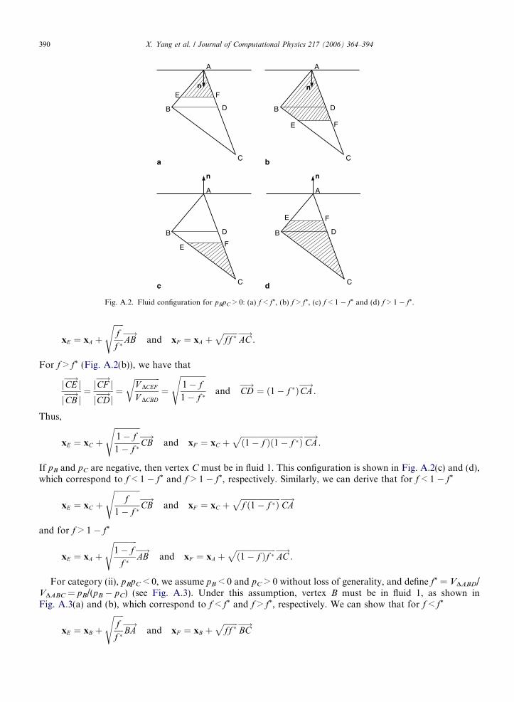
n

A

B

C

D

E F

E F

n

A

B

C

D

E F

n

A

B

C

D

E F

n

A

B

C

D

a b

c d

Fig. A.2. Fluid configuration for pBpC > 0: (a) f < f*, (b) f > f*, (c) f < 1 � f* and (d) f > 1 � f*.


xE ¼ xA þffiffiffiffiffiff �

sAB�!

and xF ¼ xA þffiffiffiffiffiffiffiff �

pAC�!

.

For f > f* (Fig. A.2(b)), we have that

jCE�!jjCB�!j ¼

jCF�!jjCD�!j ¼

ffiffiffiffiffiffiffiffiffiffiffiffiffiV DCEF

V DCBD

r¼

ffiffiffiffiffiffiffiffiffiffiffiffiffi1� f1� f �

sand CD

�! ¼ ð1� f �ÞCA�!

.

Thus,

xE ¼ xC þffiffiffiffiffiffiffiffiffiffiffiffiffi1� f1� f �

sCB�!

and xF ¼ xC þffiffiffiffiffiffiffiffiffiffiffiffiffiffiffiffiffiffiffiffiffiffiffiffiffiffiffiffiffiffiffiffið1� f Þð1� f �Þ

pCA�!

.

If pB and pC are negative, then vertex C must be in fluid 1. This configuration is shown in Fig. A.2(c) and (d),which correspond to f < 1 � f* and f > 1 � f*, respectively. Similarly, we can derive that for f < 1 � f*

xE ¼ xC þffiffiffiffiffiffiffiffiffiffiffiffiffi

f1� f �

sCB�!

and xF ¼ xC þffiffiffiffiffiffiffiffiffiffiffiffiffiffiffiffiffiffiffiffif ð1� f �Þ

pCA�!

and for f > 1 � f*

xE ¼ xA þffiffiffiffiffiffiffiffiffiffiffiffi1� f

f �

sAB�!

and xF ¼ xA þffiffiffiffiffiffiffiffiffiffiffiffiffiffiffiffiffiffiffiffið1� f Þf �

pAC�!

.

For category (ii), pBpC < 0, we assume pB < 0 and pC > 0 without loss of generality, and define f* = VDABD/VDABC = pB/(pB � pC) (see Fig. A.3). Under this assumption, vertex B must be in fluid 1, as shown inFig. A.3(a) and (b), which correspond to f < f* and f > f*, respectively. We can show that for f < f*

xE ¼ xB þffiffiffiffiffiff �

sBA�!

and xF ¼ xB þffiffiffiffiffiffiffiff �

pBC�!

n

A

B

C

D

E F

n

A

B

C

DE

a b

F

Fig. A.3. Fluid configuration for pB < 0 and pC > 0: (a) f 6 f* and (b) f > f*.


and for f > f*

xE ¼ xC þ

ffiffiffiffiffiffiffiffiffiffiffiffiffi1� f1� f �

sCA�!

and xF ¼ xC þffiffiffiffiffiffiffiffiffiffiffiffiffiffiffiffiffiffiffiffiffiffiffiffiffiffiffiffiffiffiffiffið1� f Þð1� f �Þ

pCB�!

.

For category (iii), we assume pB 6¼ 0 and pC = 0 without loss of generality. The fluid configuration is shownin Fig. A.4(a) and (b), which correspond to pB < 0 and pB > 0, respectively. We can show that for pB < 0

xE ¼ xB þffiffiffif

pBA�!

and xF ¼ xB þffiffiffif

pBC�!

and for pB > 0

xE ¼ xB þffiffiffiffiffiffiffiffiffiffiffiffi1� f

pBA�!

and xF ¼ xB þffiffiffiffiffiffiffiffiffiffiffiffi1� f

pBC�!

.

The resulting piecewise linear interface conserves the volume of fluid exactly. The method is analytical, effi-cient, and extendible to 3D. For each reconstruction, the method only requires several basic algebraic oper-ations, one square root, and several if-else operations, compared to a number of operations that is unknown apriori in iterative methods. Further details and a 3D algorithm are formulated in [38].

Appendix B. Sutherland–Hodgeman polygon clipping

In this appendix, we describe briefly the Sutherland–Hodgeman polygon clipping algorithm [42] used inSection 2.2.3. The basic idea of this algorithm is to ‘‘trim’’ the subject polygon, which is to be clipped againstthe clip polygon, by each extended edge of the clip polygon. In our case, the subject polygon is a Lagrangianfluid region that is occupied by fluid 1, and the clip polygon is a triangular Eulerian grid cell. The clip polygonmust be convex for this algorithm, which is satisfied in our case because all the grid cells are convex. As anexample, Fig. B.1 illustrates the clipping of a four-sided polygonal fluid element p1p2p3p4 against a triangulargrid cell q1q2q3, where p1p2p3p4 is trimmed by the three extended edges of q1q2q3 in order, as shown in Figs.B.1(b), (c), and (d), respectively.

n

A

B

C

E

n

A

B

C

E

a b

F F

Fig. A.4. Fluid configuration for pB 6¼ 0 and pC = 0: (a) pB < 0 and (b) pB > 0.

p1

p2

p3

p4

q2

q3

q1

r1

r2

p3

p4

q2

q3

q1

r1

r2

p3

p4

q2

q3

q1

r1

r2

p3

r4

q2

q3

q1

r3

r1

r2

p3

r4

q2

q3

q1

r3

a b

c d e

Fig. B.1. Clipping of a four-sided polygonal fluid element against a triangular grid cell. (a) The polygons before clipping. (b) Clipping ofp1p2p3p4 against edge q1q2. (c) Clipping of r1r2p3p4 against edge q2q3. (d) Clipping of r1r2p3p4 against edge q3q1. (e) The polygons afterclipping.


To illustrate the ‘‘trimming’’ process, let us consider the clipping of p1p2p3p4 against the first edge q1q2 forexample, which will result in a clipped polygon r1r2p3p4 (see Fig. B.1(b)). For convenience, we name the infi-nitely-long line, obtained by extending edge q1q2, L, and define that a vertex pj is on the ‘‘right’’ side of L if pj

is on the same side of L as the other vertex q3 is, and is on the ‘‘left’’ side otherwise. Then, the trimming pro-cess can be described as in Algorithm 1.

Algorithm 1. Trimming a polygon by a line.

for each vertex pair pj, pj+1 of the subject polygon
if both pj and pj+1 are on the right side of L then
Add pj+1 to the list of the vertices of the clipped polygon.else if pj is on the right and pj+1is on the left then

Add the intersection of the line segment pjpj+1 and L to the list of the vertices of the clipped polygon.else if pj is on the left and pj+1is on the right then

Add both the intersection and vertex pj+1 to the list of the vertices of the clipped polygon.else

Do nothing.end if

end for

The list of the vertices produced from the trimming process defines the clipped polygon, that is r1r2p3p4 for thisexample. In general, the trimming process is reentered to clip the previously clipped polygon against the sub-sequent edges of the grid cell, and the overall clipping completes as soon as the polygon has been trimmed byall the edges of the grid cell.

References

[1] F.H. Harlow, J.E. Welch, Numerical calculation of time-dependent viscous incompressible flow of fluid with free surface, Phys. Fluids8 (12) (1965) 2182–2189.


[2] S.J. Osher, J.A. Sethian, Fronts propagating with curvature dependent speed: algorithms based on Hamilton–Jacobi formulations, J.Comput. Phys. 79 (1988) 12–49.

[3] J.A. Sethian, P. Smereka, Level set methods for fluid interfaces, Annu. Rev. Fluid Mech. 35 (2003) 341–372.[4] S. Osher, R.P. Fedkiw, Level set methods: an overview and some recent results, J. Comput. Phys. 169 (2001) 463–502.[5] C.W. Hirt, B.D. Nichols, Volume of fluid (VOF) method for the dynamics of free boundaries, J. Comput. Phys. 39 (1981) 201–225.[6] W.J. Rider, D.B. Kothe, Reconstructing volume tracking, J. Comput. Phys. 141 (1998) 112–152.[7] R. Scardovelli, S. Zaleski, Direct numerical simulation of free-surface and interfacial flow, Annu. Rev. Fluid Mech. 31 (1999) 567–

603.[8] S.O. Unverdi, G. Tryggvason, A front-tracking method for viscous, incompressible, multi-fluid flows, J. Comput. Phys. 100 (1992)

25–37.[9] G. Tryggvason, B. Bunner, A. Esmaeeli, D. Juric, N. Al-Rawahi, W. Tauber, J. Han, S. Nas, Y.-J. Jan, A front-tracking method for

the computations of multiphase flow, J. Comput. Phys. 169 (2001) 708–759.[10] V.E. Badalassi, H.D. Ceniceros, S. Banerjee, Computation of multiphase systems with phase field models, J. Comput. Phys. 190

(2003) 371–397.[11] J.S. Kim, K. Kang, J. Lowengrub, Conservative multigrid methods for Cahn–Hilliard fluids, J. Comput. Phys. 193 (2004) 511–543.[12] D. Jacqmin, Calculation of two-phase Navier–Stokes flows using phase-field modeling, J. Comput. Phys. 155 (1999) 96–127.[13] D.M. Anderson, G.B. McFadden, A.A. Wheeler, Diffuse-interface methods in fluid mechanics, Annu. Rev. Fluid Mech. 30 (1998)

139–165.[14] B.J. Keestra, P.C.J.V. Puyvelde, P.D. Anderson, H.E.H. Meijer, Diffuse interface modeling of the morphology and rheology of

immiscible polymer blends, Phys. Fluids 15 (9) (2003) 2567–2575.[15] W.J. Rider, D.B. Kothe, Stretching and tearing interface tracking methods, Tech. Rep. AIAA 95-1717, AIAA, the 12th AIAA CFD

Conference, San Diego, 1995.[16] M. Sussman, P. Smereka, S. Osher, A level set approach for computing solutions to incompressible two-phase flow, J. Comput. Phys.

114 (1994) 146–159.[17] M. Sussman, E. Fatemi, P. Smereka, S. Osher, An improved level set method for incompressible two-phase flows, Comput. Fluids 27

(1998) 663–680.[18] M. Sussman, E. Fatemi, An efficient, interface-preserving level set redistancing algorithm and its application to interfacial

incompressible fluid flow, SIAM J. Sci. Comput. 20 (4) (1999) 1165–1191.[19] S.J. Mosso, B.K. Swartz, D.B. Kothe, R.C. Ferrell, A parallel, volume-tracking algorithm for unstructured meshes, in: Parallel

Computational Fluid Dynamics’96, Italy, 1996.[20] G.R. Price, G.T. Reader, R.D. Rowe, J.D. Bugg, A piecewise parabolic interface calculation for volume tracking, in: Proceedings of

the Sixth Annual Conference of the Computational Fluid Dynamics Society of Canada, vol. VIII, 1998, pp. 71–77.[21] Y. Renardy, M. Renardy, PROST: a parabolic reconstruction of surface tension for the volume-of-fluid method, J. Comput. Phys.

183 (2002) 400–421.[22] I. Ginzburg, G. Wittum, Two-phase flows on interface refined grids modeled with VOF, staggered finite volumes, and spline

interpolants, J. Comput. Phys. 166 (2001) 302–335.[23] R. Scardovelli, S. Zaleski, Interface reconstruction with least-square fit and split Eulerian–Lagrangian advection, Int. J. Numer.

Methods Fluids 41 (2003) 251–274.[24] K. Shahbazi, M. Paraschivoiu, J. Mostaghimi, Second order accurate volume tracking based on remapping for triangular meshes, J.

Comput. Phys. 188 (2003) 100–122.[25] N. Ashgriz, T. Barbat, G. Wang, A computational Lagrangian–Eulerian advection remap for free surface flows, Int. J. Numer.

Methods Fluids 44 (2004) 1–32.[26] D.B. Kothe, W.J. Rider, S.J. Mosso, J.S. Brock, Volume tracking of interfaces having surface tension in two and three dimensions,

Tech. Rep. AIAA 96-0859, AIAA, the 34th Aerospace sciences meeting and exhibit, 1996.[27] M.W. Williams, D.B. Kothe, E.G. Puckett, Convergence and accuracy of kernel-based continuum surface tension models, in:

Proceedings of the Thirteenth US National Congress of Applied Mechanics, Gainesville, FL, 1998.[28] M. Sussman, E.G. Puckett, A coupled level set and volume-of-fluid method for computing 3d and axisymmetric incompressible two-

phase flows, J. Comput. Phys. 162 (2000) 301–337.[29] M. Sussman, A second order coupled level set and volume-of-fluid method for computing growth and collapse of vapor bubbles, J.

Comput. Phys. 187 (2003) 110–136.[30] D. Enright, R. Fedkiw, J. Ferziger, I. Mitchell, A hybrid particle level set methods for improved interface capturing, J. Comput. Phys.

183 (2002) 83–116.[31] E. Aulisa, S. Manservisi, R. Scardovelli, A mixed markers and volume-of-fluid method for the reconstruction and advection of

interfaces in two-phase and free-boundary flows, J. Comput. Phys. 188 (2003) 611–639.[32] D. Greaves, A quadtree adaptive method for simulating fluid flows with moving interfaces, J. Comput. Phys. 194 (2004) 35–56.[33] M. Sussman, A parallelized, adaptive algorithm for multiphase flows in general geometries, J. Comput. Struct. 83 (2005)

435–444.[34] M. Sussman, M.Y. Hussaini, K. Smith, R.-Z. Wei, A second order adaptive sharp interface method for incompressible multiphase

flow, in: Proceedings of the Third International Conference on Computational Fluid Dynamics, Toronto, Canada, 2004.[35] A. Anderson, X. Zheng, V. Cristini, Adaptive unstructured volume remeshing-I: the method, J. Comput. Phys. 208 (2005) 616–625.[36] X. Zheng, J. Lowengrub, A. Anderson, V. Cristini, Adaptive unstructured volume remeshing-II: application to two- and three-

dimensional level-set simulations of multiphase flow, J. Comput. Phys. 208 (2005) 626–650.


[37] V. Cristini, J. Blawzdziewicz, M. Loewenberg, An adaptive mesh algorithm for evolving surfaces: simulations of drop breakup andcoalescence of interfaces in two-phase and free-boundary flows, J. Comput. Phys. 168 (2001) 445–463.

[38] X. Yang, A.J. James, Analytic relations for reconstructing piecewise linear interfaces in triangular and tetrahedral grids, J. Comput.Phys., in press, doi:10.1016/j.jcp.2005.09.002.

[39] B. Cockburn, S. Hou, C.-W. Shu, The Runge–Kutta local projection discontinuous Galerkin finite element method for conservationlaws IV: the multidimensional case, Math. Comput. 54 (1990) 545–581.

[40] B. Cockburn, C.-W. Shu, Runge–Kutta discontinuous Galerkin methods for convection-dominated problems, J. Sci. Comput. 16(2001) 173–261.

[41] A.V. Gelder, Efficient computation of polygon area and polyhedron volume, in: A.W. Paeth (Ed.), Graphics Gems V, AcademicPress, 1995, pp. 35–41.

[42] I.E. Sutherland, G.W. Hodgeman, Reentrant polygon clipping, Communications of the ACM 17 (1) (1974) 32–42.[43] K. Weiler, P. Atherton, Hidden surface removal using polygon area sorting, in: SIGGRAPH, 1977, pp. 214–222.[44] D.N. Arnold, F. Brezzi, M. Fortin, A stable finite element for the Stokes equations, Calcolo 21 (1984) 337–344.[45] H.C. Elman, G.H. Golub, Inexact and preconditioned Uzawa algorithms for saddle point problems, SIAM J. Numer. Anal. 31 (6)

(1994) 1645–1661.[46] J.E. Pilliod, E.G. Puckett, Second-order accurate volume-of-fluid algorithms for tracking material interfaces, J. Comput. Phys. 199 (2)

(2004) 465–502.[47] S.T. Zalesak, Fully multidimensional flux-corrected transport algorithms for fluids, J. Comput. Phys. 31 (1979) 335–362.[48] J. Lopez, J. Hernandez, P. Gomez, F. Faura, A volume of fluid method based on multidimensional advection and spline interface

reconstruction, J. Comput. Phys. 195 (2004) 718–742.[49] M. Rudman, Volume-tracking methods for interfacial flow calculations, Int. J. Numer. Methods Fluids 24 (1997) 671–691.[50] J.B. Bell, P. Colella, H.M. Glaz, A second order projection method of the incompressible Navier–Stokes equations, J. Comput. Phys.

85 (1989) 257–283.[51] R.J. Leveque, High-resolution conservative algorithms for advection in incompressible flow, SIAM J. Numer. Anal. 33 (1996) 627–

665.[52] E. Aulisa, S. Manservisi, R. Scardovelli, A surface marker algorithm coupled to an area-preserving marker redistribution method for

three-dimensional interface tracking, J. Comput. Phys. 197 (2004) 555–584.[53] G.I. Taylor, The formation of emulsions in definable fields of flow, Proc. R. Soc. Lond. Ser. A 146 (1934) 501–523.[54] B.J. Bentley, L.G. Leal, An experimental investigation of drop deformation and breakup in steady, two-dimensional linear flow, J.

Fluid Mech. 167 (1986) 241–283.[55] Y.T. Hu, D.J. Pine, L.G. Leal, Drop deformation, breakup, and coalescence with compatibilizer, Phys. Fluids 12 (3) (2000) 484–489.[56] M. Siegel, Cusp formation for time-evolving bubbles in two-dimensional Stokes flow, J. Fluid Mech. 412 (2000) 227–257.[57] H.A. Stone, Dynamics of drop deformation and breakup in viscous fluids, Annu. Rev. Fluid Mech. 26 (1994) 65–102.[58] A.J. James, J. Lowengrub, A surfactant-conserving volume-of-fluid method for interfacial flows with insoluble surfactant, J. Comput.

Phys. 201 (2004) 685–722.[59] X. Yang, A.J. James, An arbitrary Lagrangian–Eulerian method for interfacial flows with insoluble surfactants, in preparation.

http://dx.doi.org/10.1016/j.jcp.2005.09.002

an adaptive coupled level-set/volume-of-ﬂuid interface...

Documents