Paper No. 1569383447 1

Abstract—This paper will describe a numerical approach to

simulating biologically-plausible spiking neural networks. These are time dependent neural networks with realistic models for the neurons (Hodgkin-Huxley). In addition the learning is biologically plausible as well, being a Hebbian approach based on spike timing dependent plasticity (STDP). To make the approach very general and flexible, neurogenesis and synaptogenesis have been implemented, which allows the code to automatically add or remove neurons (or synapses) as required. Index Terms: Computational Neuroscience, Neural Plasticity, & Connectionist Approaches

I. INTRODUCTION raditional rate-based neural networks and the newer spiking neural networks have been shown to be very

effective for some tasks, but they have problems with long term learning and "catastrophic forgetting." Once a network is trained to perform some task, it is difficult to adapt it to new applications. To do this properly, one can mimic processes that occur in the human brain: neurogenesis and synaptogenesis, or the birth and death of both neurons and synapses. To be effective, however, this must be accomplished while maintaining the current memories. There have been many other examples of adaptive or evolving neural networks. Grossberg's adaptive resonance theory (ART) [1] is one of the most well-known. There are also self organizing maps (SOM) [2]. Evolving connectionist systems are discussed in [3] and evolving spiking neural networks are discussed in [4]. Many of these are summarized in Haykin's book [5] and a review paper by Widrow [6]. The adaptive part of the approach discussed here is the ability to add and remove neurons and synapses. In this paper we will describe a new computational approach that uses neurogenesis and synaptogenesis to continually learn and grow. Neurons and synapses can be added and removed from the simulation while it runs. The learning is accomplished using a variant of the spike time dependent plasticity method, which we have recently developed [7]. This Hebbian learning algorithm uses a combination of homeostasis of synapse weights, spike timing, and stochastic forgetting to achieve stable and efficient

Manuscript received Nov. 16, 2010. Lyle N. Long is with the Pennsylvania State University, University Park,

PA 16802 USA (phone: 814-865-1172; fax: 814-865-7092; e-mail: lnl@ psu.edu).

learning. The approach is not only adaptable, but it is also scalable to very large systems (billions of neurons). Also, it has the capability to remove synapses which have very low strength, thus saving memory. There are several issues when implementing neurogenesis and synaptogenesis in a spiking code. Though they may seem different, they are actually a coupled phenomenon. When several synapses die, it may lead to a neuron which has no synapses and thus require its removal. Conversely, a neurons death may require updating of

synaptic information of all neurons it was connected to. These issues and efficient ways to address them will be discussed. The neuron model that we use is the Hodgkin-Huxley model. Our previous work [7] used leaky integrate and fire neurons.

II. APPROACH The approach used here is based on the Hodgkin-Huxley

(HH) neuron model [8], which uses four coupled, nonlinear ordinary differential equations with very complex coefficients to model each neuron:

The above equations are solved using a simple forward Euler approach, which requires a time step size of roughly 0.001 mSec. While we have used leaky integrate and fire neurons in the past [7], they are rather crude approximations to biological neurons. In particular, the spikes are manually generated whenever the potential crosses some threshold. In the HH model the spikes are produced naturally. Additional comparisons of neuron models and numerical algorithms can be found in [9], where we compare the speed of various methods.

An Adaptive Spiking Neural Network with Hebbian Learning

Lyle N. Long, Senior Member, IEEE

T

Paper No. 1569383447 2

The algorithms have been implemented using an object-oriented programming (OOP) approach in C++ and are fast, efficient, and scalable. The code has "Synapse" as one of the most basic objects. These synapses each have an int that points to the neuron it receives current from (it knows the other neuron it connects to since each neuron has a list of synapses that feed into them). The Synapses also have a signed byte variable representing the weight of the synapse. So their values range form -127 to +127. Using bytes decreases the memory by a factor of four from using floats, and this is the biggest use of memory in the code (since there are usually many times more synapses than neurons). In the human brain each neuron connects to roughly 1,000-10,000 other neurons, and it has roughly 1011 neurons, so there are approximately 1014 – 1015 synapses. A mouse has roughly 10 million neurons and 81 billion synapses [10].

The code developed here also uses a "Neuron" object class with 22 float variables, 2 bool's, and 3 int's (or roughly 200 bytes/neuron for these variables). Each neuron, however, also has an array of Synapses which we can easily increase or decrease the size of during runtime. There are functions that can add or subtract neurons, and there are functions which can increase or decrease the array sizes also. The HH equations are updated by having each neuron call a method called update. Neurons can also print out their own information to the screen or save their data to a file.

The other key object or class in the code is the "Network" class. This only has two int's (numNeurons and maxNumNeurons) plus several file I/O objects for saving the state of the network and reading input. Initially maxNumNeurons is three times larger than numNeurons, but this can be adjusted at run time if more neurons are needed. The main array in the Network class is the array of Neurons, which is initially sized to maxNumNeurons. The network structured is determined at runtime by reading in a file of the form:

N neuron1 numSynapses1 SynNum11, SynNum12, ... (numSynapses1-1) neuron2 numSynapses2 SynNum21, SynNum22, ... (numSynapses2-1) neuron3 numSynapses3 SynNum31, SynNum32, ... (numSynapses3-1) . . . neuronN numSynapsesN SynNumN1, SynNumN2, ... (numSynapsesN-1)

where N=numNeurons. So any network array topology can be created quite easily. And there are utility codes that can easily create the well-known class of network architectures (e.g. all-to-all, all-to-many, etc.). The Network object is also where the learning is implemented. A Hebbian learning approach is used that has been explained elsewhere [7,11]. The approach is efficient, stable, and scalable. Homeostasis is used to keep the algorithm stable, for each neuron the sum of the weights of all the synapses is kept constant. The key to the algorithm is keeping track of the last two times that a neuron has fired (timenew and timeold). If learning is turned on, when a neuron fires then that

individual neuron calls the learn method for its synapses. It can be summarized as:

• Sum synapse weights for all neurons feeding into this neuron • For each synapse:

If timeold(PostNeuron) < timenew(PreNeuron) < timenew(PostNeuron) Weight = Weight + dWplus else Weight = Weight + dWminus

• Rescale all weights to maintain original sum of weights where:

!

dwPlus = dwMinus = 15 " edt /20

dt = timenew (PreNeuron) # timenew (PostNeuron)

This approach not only performs learning (or long term potentiation, LTP), it also implements forgetting (or long term depression, LTD). If presynaptic neurons do not contribute to the firing of the postsynaptic neuron then the synapse's weight is reduced. The learning rate factors α are used to freeze some of the synapse weights, so that previous memories are not lost. There is also a main routine in the code. The function of this routine is shown in the following flowchart:

The entire code is quite compact having only about 1500 lines of C++ code. OOP is a very effective way of implementing these neural networks. At the present time, relatively simple algorithms are used to add or remove neurons and synapses. For example, if a synapse weight is very low, it can be removed. Also, if a neuron has no synapses, it can be removed. If the output neurons have little response to the input currents, then new neurons and synapses can be added. More work is needed in this area in the future.

III. MOTIVATION The long-term goal of this work is to use these networks and algorithms to simulate human vision and object recognition, and to also try to understand brain functioning and memory. But the approaches used here are also useful for many other neural network applications (e.g. robotics sensor processing, character recognition, control systems, etc.). A simple example that helps motive this work is character recognition. For example, if we had characters represented by images of 28x28 pixels, such as in the MNIST database, we

Paper No. 1569383447 3

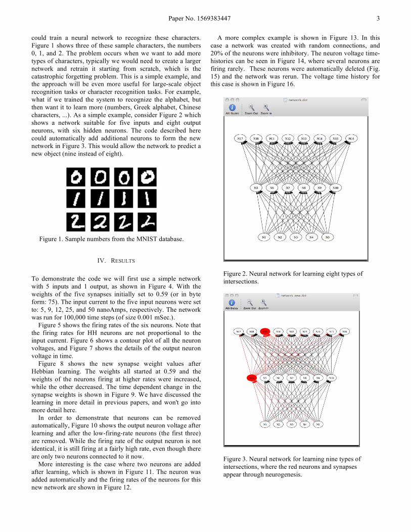
could train a neural network to recognize these characters. Figure 1 shows three of these sample characters, the numbers 0, 1, and 2. The problem occurs when we want to add more types of characters, typically we would need to create a larger network and retrain it starting from scratch, which is the catastrophic forgetting problem. This is a simple example, and the approach will be even more useful for large-scale object recognition tasks or character recognition tasks. For example, what if we trained the system to recognize the alphabet, but then want it to learn more (numbers, Greek alphabet, Chinese characters, ...). As a simple example, consider Figure 2 which shows a network suitable for five inputs and eight output neurons, with six hidden neurons. The code described here could automatically add additional neurons to form the new network in Figure 3. This would allow the network to predict a new object (nine instead of eight).

IV. RESULTS To demonstrate the code we will first use a simple network with 5 inputs and 1 output, as shown in Figure 4. With the weights of the five synapses initially set to 0.59 (or in byte form: 75). The input current to the five input neurons were set to: 5, 9, 12, 25, and 50 nanoAmps, respectively. The network was run for 100,000 time steps (of size 0.001 mSec.). Figure 5 shows the firing rates of the six neurons. Note that the firing rates for HH neurons are not proportional to the input current. Figure 6 shows a contour plot of all the neuron voltages, and Figure 7 shows the details of the output neuron voltage in time. Figure 8 shows the new synapse weight values after Hebbian learning. The weights all started at 0.59 and the weights of the neurons firing at higher rates were increased, while the other decreased. The time dependent change in the synapse weights is shown in Figure 9. We have discussed the learning in more detail in previous papers, and won't go into more detail here. In order to demonstrate that neurons can be removed automatically, Figure 10 shows the output neuron voltage after learning and after the low-firing-rate neurons (the first three) are removed. While the firing rate of the output neuron is not identical, it is still firing at a fairly high rate, even though there are only two neurons connected to it now. More interesting is the case where two neurons are added after learning, which is shown in Figure 11. The neuron was added automatically and the firing rates of the neurons for this new network are shown in Figure 12.

A more complex example is shown in Figure 13. In this case a network was created with random connections, and 20% of the neurons were inhibitory. The neuron voltage time-histories can be seen in Figure 14, where several neurons are firing rarely. These neurons were automatically deleted (Fig. 15) and the network was rerun. The voltage time history for this case is shown in Figure 16.

Figure 1. Sample numbers from the MNIST database.

Figure 2. Neural network for learning eight types of intersections.

Figure 3. Neural network for learning nine types of intersections, where the red neurons and synapses appear through neurogenesis.

Paper No. 1569383447 4

Figure 4. Simple 5-1 Network.

Figure 5. Firing rates of neurons in 5-1 network.

Figure 6. Contour plot of neuron voltages vs. time step.

Figure 7. Output neuron voltage from 5-1 network.

Figure 8. Synapse weights after Learning

Figure 9. Change of synapse weights in time due to

Hebbian learning.

Paper No. 1569383447 5

Figure 10. Output neuron voltage after removal of

neurons 1, 2, and 3.

Figure 11. 5-1 network structure after neuron N6 has

been added.

Figure 12. Firing rates of neurons in new network.

Figure 13. 20-neuron network with random connections.

Figure 14. 20-neuron network voltages.

Figure 15. New network after 4 low-firing neurons

were removed.

Figure 16. 16-neuron network voltages after learning and removing four neurons.

Paper No. 1569383447 6

V. Memory and CPU Time The code is very efficient in terms of memory and CPU time requirements. If the number of neurons is N and the total number of synapses is S, then the computer memory requirements are roughly: memory = 200 * N + 2 * S bytes which is about as low as is possible. For cases where S>>N, the CPU time is primarily the cost of summing up the current input from each synapse, which is roughly 2 floating point operations per synapse. So we have roughly: CPU Time ≈ 2 * S * timesteps / FLOPS where FLOPS is the average floating point operations per second of the machine. A 2.4 GHz MacBook laptop ran 100 million synapses (1 million neurons) for 0.1 simulated seconds (100,000 timesteps) in 5.2 hours. So if the laptop sustained 109 FLOPS (which seems reasonable) this would agree roughly with the above formula. This case required roughly 200 MBytes of memory as well. It is important to point out that many of the complex features of the code, such as learning, take very little CPU time because they are event driven effects and occur relatively rarely. That is, learning is only activated when a neuron fires, and the rates are usually below 100 Hz (or every 0.01 seconds). This is a rare event compared to what occurs each time step (roughly 0.00001 to 0.000001 seconds). Another interesting question is how does this performance compare to biological systems? In terms of memory, it compares quite well. On a laptop with 2 GBytes of memory, we can store roughly 1 billion synapses, which is probably more than a cockroach (which has about 1 million neurons) but less than a mouse (which has about 81 billion synapses). This is about a million times smaller than a human brain, in terms of storage content. In terms of the speed of the computations, a 1 gigaflop laptop (as discussed above) ran 100 million synapses in 5.2 CPU hours which was 0.1 seconds of biological time. So for this to run in real-time, the number of synapses would need to be roughly 200,000 times smaller (or about 500 synapses). However, for very small systems the run time is not simply proportional to the number of synapses. So, in fact, a network with 55 neurons and 500 synapses ran in 7 CPU seconds for a biological time of 1 second. The above, however, is for a laptop. Larger computers could obviously run faster and simulate more neurons. For example, we have a 12-processor (Power5) IBM P570 which has 100 Gbytes of RAM. This could (ideally) store roughly 50 billion synapses (on the order of a mouse), and the ratio of CPU time to biological time might be 12 times better than the laptop. This would require parallelizing the code with either OpenMP or MPI. At the other extreme, the largest supercomputer is the Cray XT (named Jaguar) at Oak Ridge National lab (www.top500.org). This machine has 362 terabytes (3.6 * 1014 bytes) of memory and a peak speed of 1375 teraflops (1.4 * 1015 ops/second) [12]. This means its peak speed and memory exceed the human brain.

V. CONCLUSION Using C++ with dynamic arrays and pointers, we can add and remove neurons or synapses from a biologically-plausible neural network. Since it will not be possible for very large scale systems to be “wired” manually, neurogenesis and synaptogenesis are crucial. This capability will potentially help us understand biological memory systems and help with sensor processing (e.g. vision). This adaptability is also important for robotic systems which need to adapt to their environments, since complex robots will not be able to be completely programmed by humans [13].

ACKNOWLEDGMENT The author thanks John C. Collins (Penn State) for very valuable discussions.

REFERENCES [1] Grossberg, S., "How Does a Brain Build a Cognitive

Code?," Psychological Review, Vol. 87, 1980. [2] Kohonen, T., "Self Organized Formation of Topologically

Correct Feature Maps," Biological Cybernetics, Vol. 43, 1982.

[3] Kasabov, N., Evolving Connectionist Systems: The Knowledge Engineering Approach, Springer, 2007.

[4] Wysoski, S. G., "Evolving Spiking Neural Networks for Adaptive Audiovisual Pattern Recognition," Ph.D. thesis Auckland University, 2008.

[5] Haykin, S., "Neural Networks," 2nd Edition, Prentice Hall, 1999.

[6] Widrow, B. and Walach, E., "Thirty Years of Adaptive Neural Networks: Perceptron, Madaline, and Backpropagation," in Adaptive Inverse Control: A Signal Processing Approach, Reissue Edition, IEEE, 2008.

[7] Gupta, A. and Long, Lyle N., "Hebbian Learning with Winner Take All for Spiking Neural Networks", IEEE International Joint Conference on Neural Networks (IJCNN), Atlanta, Georgia, June 14-19, 2009.

[8] Hodgkin, A.L. and A. F. Huxley, "A quantitative description of ion currents and its applications to conduction and excitation in nerve membranes," Journal of Physiology, vol. 117, pp. 500-544, 1952.

[9] Long, L.N. and Fang, G., "A Review of Biologically Plausible Neuron Models for Spiking Neural Networks," AIAA InfoTech@Aerospace Conference, Atlanta, GA, April 20-22, 2010.

[10] Schuz, A. and Palm, G., "Density of neurons and synapses in the cerebral cortex of the mouse," Journal of Comparative Neurology, Vol. 286, No. 4, pp. 442 – 455.

[11] Dan, Y. and M. Poo, "Spike time dependent plasticity of neural circuits," Neuron, vol. 44, pp. 23-30, 2004.

[12] Bland A.S., Kendall R.A., Kothe D.B., Rogers J.H., Shipman G.M., "Jaguar: The World’s Most Powerful Computer," Cray User's Group (CUG) Proceedings, 2009.

[13] Long, Lyle N. and Troy D. Kelley, "A Review of Consciousness and the Possibility of Conscious Robots," Journal of Aerospace Computing, Information, and Communication, Vol. 7, No. 2, Feb., 2010.

Paper No. 1569383447 7

Lyle N. Long (BME ’76, MS ’78, DSc ’83) is a Distinguished Professor of Aerospace Engineering, Bioengineering, and Mathematics at The Pennsylvania State University. He is the Founder and Director of the Graduate Minor Program in Computational Science (www.csci.psu.edu). He was also the founding Editor-in-Chief of the Journal of Aerospace Computing, Information, and Communication. In 2007-2008 he was a Moore Distinguished Scholar at the California Institute of Technology. He has also served as a visiting scientist at Thinking Machines Corporation (1990 - 1993) and NASA Langley Research Center (1999-2000). He is a Fellow of the American Physical Society (APS) and the American Institute of Aeronautics and Astronautics (AIAA). Prof. Long has written more than 240 journal and conference papers. He has advised 18 Ph.D. students and 37 Master degree students.