an advanced assessment of ski bindingsan advanced assessment of ski bindings a major qualifying...
TRANSCRIPT

An Advanced Assessment of Ski Bindings A Major Qualifying Project Report
submitted to the Faculty
of the
WORCESTER POLYTECHNIC INSTITUTE
in partial fulfillment of the requirements for the
Degree of Bachelor of Science
by
________________________________________
Kelsey Wall
________________________________________
Brendan Walsh
Date:
Approved:
_________________________________
Professor Christopher Brown, Major Advisor

i
Abstract: The leading causes of death among skiers are uncontrollable falls and collisions, which are often caused
by a phenomenon called inadvertent release. Using Nam Suh’s Axiomatic Design method, this project
focused on developing a torque-displacement system, which could determine the work required to
release a ski boot from its binding. Measuring work-to-release identifies bindings’ susceptibility to
inadvertent release through assessing its shock absorptive capabilities. However, due to the tested
displacement sensors having an unacceptably high uncertainty, ±0.68mm or greater, a work-to-release
device was not created. However, an electronic torque to release dynamometer that could be
integrated with several identified displacement methods, was designed, manufactured, and tested. The
device measured values within ±3.2 Nm of clockwise applied moments, within ±3.06 Nm of
counterclockwise applied moments, and within ±52.2 Nm of moments applied in forward lean. This
system could be improved through better definition of the calibration curves used to generate torque
values.
Authorship: All design and testing was an equal collaboration between the group members, while editing was
performed by Kelsey Wall. Primary authorship of each chapter of the report is as follows:
Brendan Walsh: Ch. 4 Tolerancing, Ch. 5 Prototype Construction, Ch.7 Design Iteration
Kelsey Wall: Ch.1 Introduction, Ch. 2 Design Process, Ch.3 Physical Integration, Ch.6 Testing of the
Design, Ch.9 Conclusion
The Abstract and Ch.8 Discussion sections of the report were created through equal collaboration of the
group members.
Acknowledgements: The team would like to acknowledge
Professor Christopher Brown, for his dedicated advising
Jeffrey Elloian, for his help in configuring and troubleshooting our circuitry
Connor Morette, for instructing us on how to machine
Niravkumar Patel, for his assistance with the NDI Polaris
Richard Howell, for his guidance and input on ski binding testing
Richard Kirby, for providing information on optical mouse use for displacement measurements

ii
Contents
An Advanced Assessment of Ski Bindings ...................................................................................................... i
Abstract: ......................................................................................................................................................... i
Authorship: .................................................................................................................................................... i
Acknowledgements:....................................................................................................................................... i
Table of Figures ............................................................................................................................................. v
Table of Tables ............................................................................................................................................ vii
1. Introduction .............................................................................................................................................. 1
1.1 Objective ............................................................................................................................................. 1
1.2 Rationale ............................................................................................................................................. 1
1.3 State of the Art .................................................................................................................................... 3
1.4 Approach ............................................................................................................................................. 7
2. Design Process .......................................................................................................................................... 9
2.1 Design Constraints ............................................................................................................................ 10
2.2 Design Decomposition ...................................................................................................................... 11
2.2.1 Zero Level Decomposition ......................................................................................................... 12
2.2.2 Functional Requirement 1 ......................................................................................................... 13
2.2.3 Functional Requirement 2 ......................................................................................................... 21
3. Physical Integration ................................................................................................................................. 27
3.1 Design Matrix .................................................................................................................................... 27
4. Tolerancing .............................................................................................................................................. 28
5. Prototype Construction ........................................................................................................................... 29
6. Testing of the Final Design and Results .................................................................................................. 31
6.1 Calibration Testing for Clockwise Twist Release Testing .................................................................. 35
6.1.1 Test setup and methods for clockwise twist release testing ..................................................... 35
6.1.2 Calibration curve, results, and analysis for clockwise twist release testing .............................. 37
6.2 Calibration Testing for Counterclockwise Twist Release Testing...................................................... 41
6.2.1 Test setup and methods for counterclockwise twist release testing ........................................ 41
6.2.2 Calibration curve, results, and analysis for counterclockwise twist release testing ................. 41
6.3 Calibration Testing for Forward Bending Release Testing ................................................................ 45
6.3.1 Test setup and methods for forward bending release testing .................................................. 46

iii
6.3.2 Calibration curve, results, and analysis for forward bending release testing............................ 48
6.4 SBB System Testing for Clockwise and Counterclockwise Release Testing ...................................... 51
6.4.1 Clockwise testing results and analysis ....................................................................................... 52
6.4.2 Counter clockwise testing results and analysis .......................................................................... 55
6.5 Additional Calibration Curve Validation Testing for Forward Bending Testing ................................ 58
6.5.1 Testing results and analysis........................................................................................................ 58
7. Design Iteration ....................................................................................................................................... 59
7.1 Optical Mouse ................................................................................................................................... 61
7.1.1 Design Decomposition ............................................................................................................... 61
7.1.2 Shortcomings of Optical Mouse ................................................................................................. 62
7.2 NDI Polaris ......................................................................................................................................... 63
2.2.1 Design Decomposition ............................................................................................................... 64
7.2.2 Shortcomings of NDI Polaris ...................................................................................................... 65
7.3 Additional Displacement Sensors ..................................................................................................... 65
7.3.1 Rotary and String Potentiometers ............................................................................................. 65
7.3.2 Rotary Encoders ......................................................................................................................... 66
7.3.3 Leap Motion ............................................................................................................................... 67
8. Discussion ................................................................................................................................................ 68
8.1 Satisfaction of the Objective ............................................................................................................. 68
8.1 Results and Satisfaction of Constraints ............................................................................................. 68
8.3 Impact of Solution ............................................................................................................................. 70
8.4 Future Recommendations ................................................................................................................ 71
9. Conclusions ............................................................................................................................................. 71
Appendix B: Axiomatic Design Concepts .................................................................................................... 76
Appendix C: Supplements to Our Approach ............................................................................................... 78
Appendix D: CAD Drawings of System ........................................................................................................ 80
Appendix E: SignalExpress Instructions (NI, 2010) ...................................................................................... 86
Appendix F: Clockwise SBB System Torque vs. Time Graph ....................................................................... 88
Appendix G: Counter Clockwise SBB System Torque vs. Time Graph......................................................... 89
Appendix H: Optical Mouse Data Analysis .................................................................................................. 90
H.1 Testing Setup and Procedure ........................................................................................................... 91
H.1.1 Labview Program for Tracking Mouse Position ......................................................................... 91

iv
H.1.2 Physical Testing Setup ............................................................................................................... 92
H.1.3 Data and Analysis ...................................................................................................................... 93
H.1.4 Findings ...................................................................................................................................... 96
Appendix I: Polaris Measurement Analysis ................................................................................................. 98
I.1 Test Setup .......................................................................................................................................... 98
I.2 Data and Analysis ............................................................................................................................... 99
Appendix J: Prototype and Consumer Costs ............................................................................................. 101
References ................................................................................................................................................ 102

v
Table of Figures Figure 1: Idealized Torque Displacement Curve for a Binding ( ) (Brown, 2006) .......................... 2
Figure 2: Testing Axes (ASTM, 2005) ............................................................................................................ 2
Figure 3: General Static Release Moment Tester Configuration (ASTM, 2005) ........................................... 3
Figure 4: Lipe Check Tester (Lipe et al., 1966) .............................................................................................. 4
Figure 5: Single Handle Torque Wrench (Vermont Ski, 2010) ...................................................................... 5
Figure 6: Double Sided Handle (Epitaux, 1989) ............................................................................................ 5
Figure 7: Heel Release Caused by Vertical Force at the Heel (Ski Gear, 2012) ............................................. 6
Figure 8: Tester Prototype (Merrill, 2013) .................................................................................................... 6
Figure 9: Torque tester in Bending Configuration (Left) and in Twist Configuration (Right) ...................... 13
Figure 10: DPs for Functional Requirement 1.1.1 and its Constituents (Full system far left, Exploded view
middle, Bottom piece second from right, Top Piece far right) ................................................................... 15
Figure 11: DP 1.1.1.2 Cylindrical Torque Applicator ................................................................................... 16
Figure 12: DP 1.1.1.3.2 Prosthetic foot interface ....................................................................................... 17
Figure 13: Complete circuit diagram including DPs 1.1.2.1 to 1.1.2.4 ........................................................ 18
Figure 14: Full Wheatstone bridge configuration DP 1.1.2.2 (Hoffman, 1986) .......................................... 18
Figure 15: Proper setup of the dual polarity power supply, DP 1.1.2.1 ..................................................... 19
Figure 16: SignalExpress window for tester ................................................................................................ 20
Figure 17: DPs for functional requirement 2.1.1 and its constituents (full system, right; exploded view,
left) .............................................................................................................................................................. 23
Figure 18: DP 2.1.1.2 Cylindrical torque applicator .................................................................................... 24
Figure 19: DP 2.1.2.2 full wheatstone bridge configuration (Hoffman, 1986) ........................................... 26
Figure 20: Complete circuit diagram including DPs 2.1.2.1 to 2.1.2.4 ........................................................ 26
Figure 21: Design Matrix ............................................................................................................................. 27
Figure 22: Completed device components ................................................................................................. 30
Figure 23: Completed part assembly .......................................................................................................... 30
Figure 24: Running and Recording Testing Information ............................................................................. 33
Figure 25: Clockwise calibration pulley applicator system ......................................................................... 36
Figure 26: Mean Outputs and Standard Deviations at Specified Torque Values ........................................ 38
Figure 27: Calibration Curve for Torque Applied in the Clockwise Direction ............................................. 39
Figure 28: Correlation between Applied Torque and Strain ....................................................................... 40
Figure 29: Counterclockwise torque applicator pulley system ................................................................... 41
Figure 30: Mean outputs and standard deviations at specified torque values applied in the
counterclockwise direction ......................................................................................................................... 43
Figure 31: Calibration Curve for Torque Applied in the Counter Clockwise Direction ............................... 43
Figure 32: Correlation between strain and torque applied in the counterclockwise direction ................. 45
Figure 33: Forward bending torque applicator pulley system .................................................................... 47
Figure 34: Mean outputs and standard deviations at specified forward bending torque values .............. 49
Figure 35: Calibration curve for torque applied in the forward bending direction .................................... 49
Figure 36: Correlation between strain and torque applied in forward bending ........................................ 51

vi
Figure 37: Ski Boot Binding Testing Setup for the Vermont Release Calibrator (left) and the designed
device (right) ............................................................................................................................................... 52
Figure 38: Torque to release over time for clockwise run 1 with our device ............................................. 53
Figure 39: Torque to release over time for counterclockwise run 1 with our device ................................ 56
Figure 40: Volume of Polaris measurement range (NDI, 2014) .................................................................. 64
Figure 41: Displacement measurement with string potentiometers ......................................................... 66
Figure 42: Working range of a LeapMotion (LeapMotion, 2014) ............................................................... 67
Figure 43: "Bow Effect" Inadvertent Release (Brown and Ettlinger, 1985) ................................................ 74
Figure 44: Failure of Ski to Release ............................................................................................................. 75
Figure 45: Bending Moment Sensed by the Binding vs. the Tibia (Brown and Ettlinger, 1985) ................. 75
Figure 46: Relationship Between FRs and DPs (Suh, 1990) ........................................................................ 76
Figure 47: Failure of Independence Axiom ................................................................................................. 76
Figure 48: Information Axiom Satisfied by Altering k ................................................................................. 77
Figure 49: Objectives Tree Representation of Objectives and Sub-Objectives .......................................... 78
Figure 50: MAX Configuration ..................................................................................................................... 86
Figure 51: A compilation of all torque vs time graphs generated during clockwise SBB system testing ... 88
Figure 52: A compilation of all torque vs time graphs produced during counterclockwise SBB system
testing ......................................................................................................................................................... 89
Figure 53: Labview program for documenting mouse position .................................................................. 92
Figure 54: Physical test setup for mouse position data acquisition ........................................................... 92
Figure 55: Changing the pointer speed, or sensitivity, of an optical mouse .............................................. 93
Figure 56: Mean and standard deviation of mouse displacement measurements from a 2000 DPI mouse
at pointer speed 7 ....................................................................................................................................... 96
Figure 57: Ski boot with attached passive marker and passive marker reference marker on testing bench
.................................................................................................................................................................... 98

vii
Table of Tables Table 1: Paired Functional Requirements and Design Parameters ............................................................ 12
Table 2: FR1 Determine Binding Response to tibial axis torsion ................................................................ 13
Table 3: FR 1.1 Measure torsion about z-axis accurately in time ............................................................... 14
Table 4: FR 1.1.1 Transmit torque through system for measurement ....................................................... 14
Table 5: FR 1.1.2 Acquire Strain Measurements ......................................................................................... 18
Table 6: Selection of a resistor value for a specified gain (Texas Instruments, 2005) ................................ 20
Table 7: FR 2 Determine binding response to forward bending loads ....................................................... 21
Table 8: FR 2.1 Measure torque applied about the positive y-axis in time ................................................ 22
Table 9: Transmit torque through system for measurement ..................................................................... 22
Table 10: FR 2.1.2 Acquire strain measurements ....................................................................................... 25
Table 11: Machining error analysis ............................................................................................................. 31
Table 12: FR 1.1.3 Create a strain to torque calibration curve for twist release ........................................ 32
Table 13: FR 2.1.3 Create a strain to torque calibration curve for forward bending release ..................... 32
Table 14: FR 1.2 and 2.2 Validate torque measurements........................................................................... 32
Table 15: FR 1.1.3.1 Create strain to torque calibration curves in clockwise release ................................ 36
Table 16: The relationship between the mass applied to each side of the pulley system and the applied
torque ......................................................................................................................................................... 37
Table 17: Relative Rang of Output Values from Clockwise Testing ............................................................ 38
Table 18: Percent Difference and Relative Rang of Torque Testing in the Clockwise Direction ................ 39
Table 19: Relative range of output values from counterclockwise testing ................................................ 42
Table 20: Percent Difference and Relative Rang of Torque Measurements in the Counter Clockwise
Direction ...................................................................................................................................................... 44
Table 21: Create strain to torque calibration curve in forward bending release ....................................... 46
Table 22: The relationship between the applied mass and the applied torque ......................................... 47
Table 23: Relative range of output values from forward bending testing ................................................. 48
Table 24: Percent Difference and Relative Range of Torque in the Forward Bending Direction ............... 50
Table 25: Characterization of torque to release measurements from a Vermont Release Calibrator and
the designed device .................................................................................................................................... 53
Table 26: Percent difference and relative range of the Vermont Release Calibrator and the designed
device .......................................................................................................................................................... 54
Table 27: Characterization of torque to release measurements from a Vermont Release Calibrator and
the designed device .................................................................................................................................... 56
Table 28: Percent difference and relative range of the Vermont Release Calibrator and the designed
device .......................................................................................................................................................... 57
Table 29: Percent difference and relative range of the forward bending calibration curve at 148.6 Nm of
applied torque............................................................................................................................................. 59
Table 30: Displacement sensor comparison ............................................................................................... 60
Table 31: Initial decomposition for torque-displacement binding tester ................................................... 61
Table 32: Decomposition for a displacement measurement system utilizing an optical mouse ............... 62

viii
Table 33: Decomposition for a displacement measuring system utilizing the NDI Polaris ........................ 64
Table 34: Satisfaction of project constraints .............................................................................................. 68
Table 35: Pairwise Comparison Chart of Objectives ................................................................................... 79
Table 36: Terminal/pin locations ................................................................................................................ 87
Table 37: Location for software tutorials .................................................................................................... 87
Table 38: Mouse position and linear displacement calculations ................................................................ 94
Table 39: Displacement measurements obtained by a standard mouse at pointer speed 1 ..................... 94
Table 40: Displacement measurements obtained by a standard mouse at pointer speed 5 ..................... 95
Table 41: Displacement measurements obtained by a standard mouse at pointer speed 10 ................... 95
Table 42: Displacement measurement from a 2000 DPI mouse at pointer speed 7 .................................. 96
Table 43: Polaris position tracking of a ski boot ......................................................................................... 99
Table 44: Average Polaris Error (cm) ........................................................................................................ 100

1
1. Introduction
1.1 Objective The objective of this Major Qualifying Project is to design an alpine ski binding testing device that
measures the torque, displacement, and work to release ski boots from bindings in response to multiple
quasi-static loading configurations in the y and z axis. The test device would be able to identify ski
binding devices’ susceptibility for inadvertent release [Appendix A].
1.2 Rationale
On average forty-one people die per year in skiing accidents, while another forty-four sustain serious
injuries such as paralysis or head trauma (Hawks, 2012). However, in 2012 there was a 32% increase in
fatalities and a 17% percent increase in severe injuries. The leading causes of death among skiers are
uncontrollable falls and collisions (Lagran, 2012), which are often caused by a phenomenon called
inadvertent release (Ettlinger et al., 2005). Inadvertent release is one of the two modes of failure for the
ski-binding-boot system (SBB) (Shealy et al., 1999). In this type of failure the binding releases the boot
from the ski at an unnecessary or inappropriate time, when the load is not large enough to cause injury
(Ettlinger et al., 2005). The other mode of failure deemed a “miss”, is when the binding fails to release
under an injurious load, often resulting in tibial fractures and other lower leg injuries (Shealy et al.,
1999). A thirty year study found that the rates of both inadvertent releases and “misses” have increased
in the last 15 years (Ettlinger et al., 2005). However, the rate of inadvertent releases was found to be 2.3
times higher than “misses” in the 17-49 age group, which composes 76.3% of the skiing population.
Creating a binding testing device that could measure work to release is important because it could help
identify if bindings are prone to inadvertent release.
Inadvertent release can be caused by retention problems, inherent flaws in the heel piece design, skier
error, as well as issues with release torque [Appendix A] (Ettlinger et al., 2009). The unavailability of
binding testers that can identify issues with more than just the release torque leads to under evaluated
bindings going on the slopes and resulting in injuries. Some skiers’ ignorance to the mechanisms of
inadvertent release also leads them to needlessly elevate their release torques to dangerously high
levels (Ettlinger, 2010). They do this to prevent inadvertent release when in fact they only put
themselves at risk for severe lower leg injuries. Developing a binding tester that could determine the
work to release would allow for ski-binding retention capabilities to be analyzed in a new way. Work to

2
release indicates a way to measure the anti-shock capabilities of SBB systems because it is a measure of
the work a binding can absorb from its
environment before release [Figure 1] (Brown,
2006). Work to release is defined as the integral
of torque in terms of displacement, or simply the
area under the torque displacement curve. The
work to release can be increased by increasing
the displacement up to the release point. In this
manner the binding could prevent inadvertent
releases caused by instantaneous large torques.
This would be especially beneficial in the case of the bow effect (Brown and Ettlinger, 1985; Young,
1989) where the heel piece senses a higher moment than the tibia due to an instantaneous force
experienced by the shovel of the ski couple with forward lean of the skier. In an ideal situation
displacement would occur above the torque limit necessary for control (Tcon ), so that steering forces
applied by the skier’s legs under normal conditions would not be dampened, but below the injury
threshold (Tinj.). By creating a device that measures work to release the ski boot binding system could be
analyzed in a way that would identify issues with retention as well as release. This could lead to
improvements in binding designs that would mitigate
the danger of inadvertent releases. Currently, there
are limited means to test for work to release; testing
options are available, but they are prohibitively
expensive and used to test bindings before they are
put onto the market (ISO, 2009). There are currently
no testing devices available for ski shop or average
consumer usage. The objective of this project is to
address this gap in technology by designing a binding test device that finds torque to release as well as
release displacement. We will find torque to release in the y and z aixs [Figure 2]. The torques
experienced around the y axis correspond to forward and backward lean of the skier and are the
mechanism for vertical boot release at the heel. The torques experienced around the z axis correspond
to tibia torsion and are responsible for the clockwise and counterclockwise release of the boot at the
toe. We will also be taking angular displacement measurements in the xy and xz planes. Angular
displacement in the xy plane corresponds to the displacement of the boot in the binding during applied
Figure 1: Idealized Torque Displacement Curve for a Binding ( ∫ ) (Brown, 2006)
Figure 2: Testing Axes (ASTM, 2005)

3
twist torques. The angular displacement of the boot in the xz plane corresponds to the displacement of
the boot in the binding during forward or backward lean and subsequent heel release. Valgus torques
along the x axis, commonly attributed to knee injuries (Dodge et al, 2010), are rarely addressed in SBB
systems and are not addressed in current commercial binding testers. Due to this we will not be
measuring torque to release, displacement, or work to release in regards to the x axis.
1.3 State of the Art
Alpine skiing is an extremely popular sport, with over 8 million participants in the United States alone in
the year 2013 (SIA, 2013). However, due to the high velocities experienced, it can be a dangerous
activity. Major causes of serious ski injuries are inadvertent release, or pre-release, of the boot from the
binding, as well as failure of the binding to release under injurious loads [Appendix A]. These forms of ski
boot binding (SBB) failure can be contributed to problems with either the release or retention
characteristics of a binding (Shealy et al., 1999). Release is defined as a SBB’s ability to release the boot
from the binding at a pre-set release torque, while retention is the ability of the binding to maintain the
boot in the binding under non-injurious loading situations. There can be an appropriate release
response combined with an inappropriate retention response when a binding releases under a large
instantaneous load that would not have resulted in a lower leg injury. However, most of the binding
testers available to consumers and ski shops only have the ability to measure release, or a binding’s
ability to release at a desired pre-set torque threshold, not retention. A work to release binding tester
would be able to measure the shock absorptive capabilities of a binding, and thus its retention
capabilities, but these tests are unavailable to the general public and are only used to initially verify a
binding. Our proposed design would make it easier to identify the retention capabilities of individual
bindings and provide a new metric for safety in ski bindings that could lead to newer, safer, and more
marketable ski binding designs.
There are many different types of test mechanisms used
to test ski binding release. ASTM F504-05 outlines the
general method of testing static release moments [Figure
3], which is what is tested with modern ski binding testers
found in ski shops (ASTM, 2005). The basic test for static
release is to apply forces to a system adapted to fit into a
ski boot firmly attached to a ski in order to apply torsional
and bending moments on the ski until it releases;
Figure 3: General Static Release Moment Tester Configuration (ASTM, 2005)

4
documenting the torques required for release. However, the standards also detail how to test for quasi-
static release moments, which more accurately identify retention. The quasi-static tests detail using a
cable and pulley system to apply pre-loads on different standardized locations on the ski. When the
preload is used it will produce a release moment that is a certain percentage of the moment in test 2.1,
which is used as a base. This serves as an indicator as to how release torques will vary based on different
loading conditions, such as forward or backward lean in a skier. Previously mentioned tests 2.3 and 2.5
are both examples of quasi-static testing in ASTM F504. Though these tests can be reliable in predicting
many different loading situations they are limited in the fact that they are only applied in specific
regions and are not subjected to dynamic testing conditions. This means that they are unable to identify
some of the possible mechanisms of release such as inadvertent release. The quasi-static tests are more
comprehensive but are not performed in ski test shops, as they are difficult to set up, require multiple
configurations for different tests, and are time intensive.
An early method of ski binding tester that pre-dated the F504 standards, and standardized release
settings, was the Lipe Check tester [Figure 4]. The Lipe Check was
invented in 1966 and pre-dates the releasable heel mechanism in
ski bindings (Lipe et al., 1966). As such the tester purely measured
toe piece release. It did this in a unique way, by measuring the
force to release the boot from the binding. When the lever arm
actuator is pulled forward, springs push a plunger against the side
of the boot. The plunger pushes against the side of the boot until
the boot releases, whereupon the force is measured through
an “O” ring’s resultant position on one of the graduation
marks that lie on the reduced diameter portion of the plunger. The number of the graduation mark that
the “O” ring lies upon on the bindings release is then compared with the preferred number given by the
designer based on weight and skier ability. This method introduced the idea of binding release testing,
but could only measure force applied. Release torque could be calculated using force times
displacement but were less accurate.
Figure 4: Lipe Check Tester (Lipe et al., 1966)

5
The Vermont Release Calibrator, originally invented in 1974, is an early
torque to release measuring device still commonly used in the United
States (Ettlinger, 1974). The Vermont Calibrator is a simple torque
wrench adapted to measure both twist release at the toe piece and
bending release at the heel piece and is currently sold at $3,975 to
$4,975 (Vermont Ski, 2010). There are three different parts to the device,
a foot, a leg, and an arm. The foot is inserted into the boot, the leg is
attached to the foot for forward/backward bending tests, and the arm is
a torque wrench that is attached to the foot for twist tests and the leg for bending tests. To perform a
twist release the foot is put in the boot and attached to the arm, the arm is held with a hand on each
end and rotated clockwise or counter clockwise until release. However, true couples are desired in twist
release tests, which is impossible when the lever arm only has one handle [Figure 5]. The idea is to get
rotation without translation, which would be better accomplished with two equally sized handles. To
perform a bending test the foot is inserted into the boot, under which a strap is placed, then the leg is
attached to the foot and the arm attached to the leg. The arm is then grabbed and pulled either forward
until release. All measurements from this device are given in Nm and can be used directly with ASTM F
939-05a standards.
A similar device to the Vermont Release Calibrator was the Epitaux binding tester, which employed a
similar lever mechanism (Epitaux, 1989). Though the Epitaux is
no longer in use it had several design improvements over the
Vermont tester. The foot mechanism that slid into the boot
was equipped with wheels that allowed for easier placement
within the boot and the handle used for the twist test used a
large two-sided handle to ensure a true couple during
testing [Figure 6]. This device also included some electrical
components that would be useful for a work displacement tester. Instead of utilizing a torque wrench
the Epitaux uses two strain gauges to gain the release torque in both the twist and bending tests. When
measuring the work to release torque to release and displacement have to be simultaneously measured
to perform a proper integration meaning that the data needs to be gained electronically so that it can be
input into a computer. The way the strain gauge works is that when torque, or rather the turning force,
is applied to the system, stress is experienced by the metal bar labeled “10” in Figure 5, this stress
Figure 5: Single Handle Torque Wrench (Vermont Ski, 2010)
Figure 6: Double Sided Handle (Epitaux, 1989)

6
causes a deformation, or strain, to the bar that is read by the gauge. The torque can be measured as it is
proportional to the strain experienced by the system.
The Speedtronic Pro tester is one of the modern binding testers
produced by Wintersteiger, that incorporates a user friendly and
predominantly hands free design (Wintersteiger, 2011). Though
these machines are uncommon in the United States they are
popular in countries such as Austria and Switzerland (Ski Gear,
2012). The testing system is completely electronic once the ski,
with the attached boot, is correctly loaded onto the
instrument, which eliminates most user error. The tester
simply enters the user weight, height, age, and skier type as well as boot sole length and binding type,
and then the machine produces the correct release settings based on the standards. The machine then
tests the binding by directly applying forces to either side of the front of the boot in the twist test, and
directly under the heel of the boot [Figure 7] in the case of the bending test. The problem with this
testing is that applying a force directly under the heel does not accurately reproduce the bending
moments generated by skier lean. This makes the heel release tests much less reliable. Another problem
with this testing device is that it is prohibitively large and expensive for most ski shops.
Despite the amount of ski binding testers and tests that have been created and are available on the
market today, none measure work to release. Recent work at Worcester
Polytechnic Institute was done on a torque-displacement binding tester
(Merrill, 2013). The tester utilized a strain gauge, fitted to a Vermont
Release Calibrator, and computer mice to input data into a Labview
program that would simultaneously measure release torque and
displacement [Figure 8]. In this project Bradley Merrill was able to prove
that computer mice have the required accuracy to measure ski-boot
displacement, and was able to identify Labview as a program that could
process torque and displacement data. Unfortunately, there was difficulty in indexing the mouse
displacement data in the software; so while data from the mouse was able to be read, it could not be
simultaneously processed with data from a strain gauge. There was also no presented data on torque to
release for the binding, though a Labview model was developed. Though there is no completed model of
Figure 7: Heel Release Caused by Vertical Force at the Heel (Ski Gear, 2012)
Figure 8: Tester Prototype (Merrill, 2013)

7
a work to release binding tester, Merrill’s work identified key requirements and possible solutions for a
successful design.
Current binding testers and standards are focused on the torque necessary for lateral toe release and
vertical release at the heel (ASTM, 2005; Vermont Ski, 2010; Wintersteiger, 2011). However, there are
retention issues, key elements in inadvertent releases, which have failed to be addressed in modern ski
binding testing technology. These issues could be addressed by a tester that not only looks at release
torques, but at the work it takes for bindings to release. If work to release could be identified, then
binding safety could be measured in a more comprehensive manner and new and more robust binding
systems could be produced. This is because an increase in work to release would mean an increase in
the amount of energy bindings could absorb before release (Brown, 2006). This would decrease or
eliminate the risk of pre-release through large instantaneous torques, such as those seen in the bow
effect (Brown and Ettlinger, 1985; Young, 1989).
1.4 Approach
Client Statement and Objectives:
Our initial client statement, Appendix C, was first refined to concentrate the focus of the project, the
final client statement is as follows.
To design an inexpensive torque and work to release binding tester that would be able to demonstrate
response to multiple quasi-static loading conditions, whose design could be downloadable off the web
and be safely usable by ski shops and ski teams.
Objectives for our project based on our client statement and ASTM and ISO standards can be viewed in
Appendix C.
Strategy:
The following strategy was used to develop our project. Using Suh’s Axiomatic design method [Appendix
B] and Acclaro software a design for a work to release binding tester that met our functional
requirements was created. Through using readily available resources and inexpensive components, or
components which have inexpensive counter-parts, we were able to create an inexpensive torque tester
that has the capability of outputting continuous torque data to a computerized system. If a further
method of measuring displacement was developed, that could be integrated into this system, the work
to release could be obtained by integrating the area under the torque/displacement curve. To the end of
displacement measurements, we have explored and described several alternatives, the Polaris Optical

8
Tracker, rotary encoders and string potentiometers, and Leap Motion optical controller. Additionally,
we created an iteration of our design that included a wireless optical mouse for displacement
measurements; however we found this design to be ineffectual for our purposes, and disproved the
optical mouse as a means of measuring displacement to release in ski-bindings.
This device was designed to interact with the prosthetic foot component of the Vermont Release
Calibrator, but have independent components that measure torque to release in twist and forward
bending. The device was also designed to be useable with any type of boot or ski type available on the
market. The torque tester for twist release was designed to withstand loads of up to 462 Nm, safety
factor of 3, and the torque tester for forward lean release was designed to withstand loads of up to
1200Nm, safety factor of 1.75. However, the methods of displacement measurement that we explored
in-depth, the optical mouse and Polaris Tracker, were not capable of measuring within 0.2 mm as per
the ISO standards for alpine ski bindings test methods (ISO, 2009). Our design prototype was
inexpensive, due to the availability of resources at Worcester Polytechnic Institute (WPI); however the
cost for customer production would be slightly higher due to outside machining costs and the need to
purchase a DAQ and Signal Express Software.
Each component of the torque tester design was modeled in SolidWorks. Manual calculations and finite
element analysis, using ANSYS Workbench, was performed to verify that the parts would not
permanently deform under the required loads, but provide enough plastic deformation for strain gauge
readings. After the torque tester parts were modeled, tool paths for the manufacturing process were
generated in Esprit. The components were machined using the HAAS CNC machine center in the
Washburn Shops at WPI. The raw data obtained through our torque testing instrument was collected by
a National Instruments (NI) DAQ and was synthesized and exported to Excel using NI Labview
SignalExpress Software. Wireless optical gaming mice were tested via Labview to determine if they
were accurate enough for displacement measurements, the feasibility of their implementation into our
design was also discussed as an option for ski boot displacement with Mr. Richard Kirby, an expert in
displacement measurements. Upon disproving the optical mice, a Polaris Tracker system was also tested
and found to be lacking in the required precision.
Specifically for toque measurements, a full Wheatstone bridge, of different configurations, was used on
both the twist and bending release testing components, and an operational amplifier was used to
enhance the differential voltage for use with our DAQ model. The amplified electrical analogue strain
signals, which were calibrated to known torque levels, were acquired through the use of a National

9
Instruments DAQ and NI Measurement and Automation Software in combination with Labview
SignalExpress software. The completed torque testers measured voltage change under an applied load
and strain. To calibrate these measurements the strain output of the testers at five known applied
torques in twist, four in bending, and at zero loading. The correct torque values were determined
through comparing anthropometric data with the ASTM standards for the selection of release torque
values (ASTM, 2005). The determined torques were applied via pulley systems designed to apply the
correct amount of torque in clockwise and counterclockwise twist release and forward lean release. The
results of this testing were plotted in Excel and a calibration curve was produced. The tester was then
used to release a ski boot from the SBB system in twist. The amount of torque needed to release the ski
from the binding was first determined through using the Vermont Release Calibrator. Then our tester
was used and output values were produced, which were analyzed with our calibration curve to predict
the applied torque. The variance between the torque to release documented by our tester compared to
the Vermont Release Calibrator was then documented and compared.
Our displacement measurements were made by applying removable fiduciaries, also known as passive
markers, onto the tested ski boot in order for the Polaris Spectra to optically track the three-dimensional
motion of the boot, while other passive markers were used to provide a reference frame for the
displacement. The position of the boot in relation to the reference marker was determined by the
Polaris’ optical measurement system and Application Program Interface (API), which allowed for
tracking of specific passive markers and output data to Excel. During Polaris testing, the position of the
tracking markers was measured and recorded via calipers, and then compared to the positions
documented by the Polaris to validate the precision of the measurements. The Polaris measurements
were not precise enough to be viable for displacement measurements in our system, and also did not
provide a time parameter, which would make it difficult to interface with our torque measurements.
2. Design Process
In this project we utilized Nam Suh’s axiomatic design theory [Appendix B], using Acclaro software for
our decompositions and matrix production. The functional requirements and their corresponding design
parameters were developed in a hierarchical fashion beginning with the main objective as Functional
Requirement 0, which acts as a parent to the subsequent requirements also known as children. This
process organizes and reduces the number of functional requirements of the system such that any set of
“children” are mutually exclusive from one another and collectively exhaustive with respects to their

10
corresponding “parent”. This creates a more robust design by helping the designer eliminate
redundancies, coupling, and complexity from within a design (Suh, 1990). Conversely, the iterative
algorithmic approach requires time consuming trial and error and relies on experience, as opposed to
rules and axioms, for evaluation.
2.1 Design Constraints Constraints:
The constraints of our project were based on industry standards for binding testers, WPI budget
restrictions, and consideration of our target audiences’ maximum budget, and were considered before
the design process was begun to ensure success in satisfying the objectives. Elements of the ASTM
F1061 performance requirements for ski binding test devices, section 6, were considered in creating the
constraints for our project and those we sought to follow are listed below (ASTM, 2008). The referenced
equations are discussed in detail in the testing section and are found in section 9 of ASTM F1062 (ASTM,
2013).
ASTM Requirements:
• Torque testing must be no greater than ±5% of the release torque determined through testing with the standard apparatus of ASTM F504, using the equation from ASTM F1062, in the Z-axis.
• Torque testing must be no greater than ±5% of the release torque determined through testing
with the standard apparatus of ASTM F504, using the equation from ASTM F1062, in the Y-axis.
However, as we were unable to test with an ASTM F504 standard testing apparatus, detailed in the state
of the art section, we were unable to measure for these values. We instead used the provided equations
and constraints to develop the constraints for our testing device.
Constraints for Calibration Testing Based on ASTM Standards:
• Torque testing must be no greater than ±5% of the known applied torque during calibration testing, using the equation from ASTM F1062, in the Z-axis.
• Torque testing must be no greater than ±5% of the known applied torque during calibration
testing, using the equation from ASTM F1062, in the Y-axis.
Constraints for Testing with a Ski Boot Binding System Based on ASTM Standards:
• Torque testing must be no greater than ±5% of the release torque determined through testing with a Vermont Release Calibrator, using the equation from ASTM F1062, in the Z-axis.
• Torque testing must be no greater than ±5% of the release torque determined through testing
with a Vermont Release Calibrator, using the equation from ASTM F1062, in the Y-axis.
We also assessed the relative range of values produced by the tester, in both calibration and SBB system
testing for all testing configurations, using a slight alteration to the equation used to calculate the

11
difference between results produced by a tester to the expected results from a calibration curve.
However, these results served as a basic assessment and have no associated constraints.
Additional Constraints:
The additional constraints of our project were based on industry standard for ski boot release, WPI
budget restrictions, and consideration of our target audiences’ maximum budget and are as follows:
• The device must be compatible with existing ski boot binding setups
• Displacement testing uncertainty must be within 0.2 mm (ASTM, 2009; ISO, 2009; ASTM E2655, 2008)
• Customer cost must be under $350 • Design prototype must be under $500
2.2 Design Decomposition
The design decomposition highlights each functional requirement developed in the design process and
explains the reasoning behind the selection of a design parameter to satisfy it. Detailed drawings of
every torque tester component can be seen in Appendix D. As a note, while most of the dimensions in
the following summary of the designed components are described in English units as well as the
drawings of the parts, as the CAM software at WPI uses the English system, the parts that interface with
the Vermont Release Calibrator prosthetic foot and the lever arm modeled after the Epitaux tester are
referred to in metric units. Information on the Vermont Release Calibrator and Epitaux tester can be
viewed in the State of the Art section. Table 1 shows the first three levels of the functional requirements
and their corresponding design parameters. Some of the FRs in our first three levels of decomposition
involved the calibration and testing of our device. These will be discussed in greater detail in Ch.6,
Testing of the Design. As the displacement measurement techniques we investigated were not suitable
they are not addressed in our final design decomposition, but decompositions of the different
displacement techniques can be found in Chapter 7, Iterations. As our tested methods for displacement
measurement did not have the required accuracy, we were unable to create a work to release tester.
Our decomposition and devise are for an inexpensive torque tester that has the capability of outputting
continuous torque data to a computerized system, which could be integrated with a future
displacement measuring device for work to release. The various testing axes referenced in the
decomposition can be seen in figure 3.
To satisfy the first axiom of axiomatic design, independence, each level of the design was collectively
exhaustive and mutually exclusive. At level one of the design we divided our design into two separate
components, the first evaluated the response of the binding in twist release, the second evaluated the

12
binding in forward bending release. This is collectively exhaustive as it evaluates both standard methods
for binding release and mutually exclusive because it evaluates two different loading configurations. The
second level of the design serves as a mean for measuring applied torque and validating these
measurements. This is collectively exhaustive as encompasses both the process of obtaining
measurement values and verifying their fulfilment of the constraints. The second level is mutually
exclusive because measuring the torque values requires a dynamometer system, while validating these
measurements requires pre-existing measurement devices and processing through Excel functions. The
third level of the design encompasses the requirements for the dynamometer and validation testing
system. All aspects of this level will be defined in detail in the following sections, but are mutually
exclusive as they are used to define separate specific requirements of the measurement or validation
process. The sum of the third level of the design fully defines the second level of the design, indicating
that the third level is collectively exhaustive.
Table 1: Paired Functional Requirements and Design Parameters
2.2.1 Zero Level Decomposition
The fundamental requirement of this design is that it should evaluate a binding’s safety by determining
if it responds appropriately to different loading situations (Shealy et al, 1999). In order to do this the
tester must identify if the binding is releasing at the desired torque value to which the binding is set, by
accurately identifying the amount of torque applied to the SBB system in twist and forward lean release.
However, torque to release alone may be insufficient to identify injurious situations from non-injurious
situations, as is the case in the “bow effect” [Appendix A] (Brown and Ettlinger, 1985; Young, 1989). This
is why the zero level DP is an electronic torque tester that would allow for continuous torque
measurements over time and later integration with a displacement tester, so that a work to release
profile could be created. A distant view of the final design in the twist configuration undergoing
calibration testing, as well as a close up view of the device in the bending configuration can be seen in
Figure 9.

13
Figure 9: Torque tester in Bending Configuration (Left) and in Twist Configuration (Right)
2.2.2 Functional Requirement 1
The first level of decomposition [Table 2] separates the different mechanisms of binding release;
satisfying the independence axiom (Suh, 1990). Bindings are subjected to torques along different axes,
which have different limits before causing injury. FR 1 is to determine the response to tibial axis torsion
applied around the z-axis (Figure 10), this functional requirement was satisfied by our twist release
tester. Functional requirement 1 was broken into two sub-FRs. The first, FR 1.1, was to measure torsion
about the z-axis accurately in time. This FR was satisfied by DP 1.1, a dynamometer system. The second
sub-FR, FR 1.2, was to validate the torque measurements, which was accomplished through DP 1.2, a
testing system that involves comparing generated torque values for our tester with those produced via a
Vermont Release Calibrator in Excel.
Testing was included in multiple levels of our design of the device. This was because testing was
necessary to establish the relationship between our collected data and known torques to be able to
determine applied torques in a SBB system and because initial validation of the system was required to
demonstrate the devices’ efficacy. In this section only FR 1.1 will be explored, as FR 1.2, validate torque
measurements, will be explained in Chapter 6, testing of the final design.
Table 2: FR1 Determine Binding Response to tibial axis torsion
FR 1.1
Functional requirement 1.1 [Table 3] was broken into four lower level functional requirements. The first
was to create a physical device that could transmit an applied load through the tester to the SBB system,

14
with a portion of this device being able to elastically deform to allow for strain gauge readings. The
second was to create a system which could collect strain information based on the elastic deformation
of the body of the tester. The third was to create a system to calibrate strain to torsion by creating a
calibration curve in both the clockwise and counterclockwise directions, which would be accomplished
through the design of a pulley system for torques applied in the clockwise and counterclockwise
directions. The fourth was to measure torque to release in the SBB system using the created calibration
curve in Excel. The third and fourth sub-functions are described in chapter 6, Testing.
Table 3: FR 1.1 Measure torsion about z-axis accurately in time
Functional Requirement 1.1.1
The decomposition of functional requirement 1.1.1 [Table 4] shows the development of the physical
components of our torque tester. The functional requirements of the physical tester were broken down
into three lower level requirements. The first, FR 1.1.1.1, describes how the tester must include a means
to apply torque to the testing applicator from which the measurements will be taken. The second, FR
1.1.1.2, indicates a need for a surface from which to measure the applied torque. This surface would
have to elastically deform in the range of applied loads to allow for torsion measurements to be
obtained, but should not plastically deform. The third, FR 1.1.1.3, describes how the tester would need
to interface with the SBB.
Table 4: FR 1.1.1 Transmit torque through system for measurement
In order to apply a load to the applicator we used DP 1.1.1.1.1, a
meter tall lever arm with a 1 meter
long handle (Figure 10). The lever arm was modeled after the Epitaux handle, which we used for testing.
This design was used because the dual handles allow for a pure couple while testing on the SBB, and the

15
1 meter length allows for mechanical advantage while applying a load to the system, facilitating testing.
The testing lever is made of two hollow stainless steel bars, each with a thickness of 2.5mm to make it
resistant to deformation, but light. The hollow cores of the bars are 15mmx25mm, which allows for the
lever arm to interface with the other components. The two bars are welded together to complete the
handle.
To interface the lever with the cylindrical torque applicator, we designed a top piece system with a
releasable pin DP 1.1.1.1.2 (Figure 10). The top piece was machined out of 2” diameter 6061 Aluminum
stock, which is a low cost alternative. The top piece included a 50mm extruded feature that was
14.97x24.97mm to form an RC1, close sliding, fit with the application lever. The cylindrical portion of the
top piece was 2” in diameter and 1” long, with a
deep and 1.52” diameter hole that allows for an RC1
fit with the cylindrical torque applicator. The top piece is attached to the torque applicator by a pin that
was purchased at McMaster Carr. The pin was 0.25” in diameter and had a 2” working length, length
between the depressible ball stopper and the chain attachment. To allow for a pin of this diameter
0.257” holes were drilled into the side of the top piece and the torque applicator 0.387” from their
respective edges.
Figure 10: DPs for Functional Requirement 1.1.1 and its Constituents (Full system far left, Exploded view middle, Bottom piece second from right, Top Piece far right)
A cylindrical torque applicator DP 1.1.1.2, is used to satisfy the functional requirement of a part that
provides a surface for strain measurements that can be calibrated to determine torque [Figure 11]. The

16
cylindrical applicator interfaces with the top piece is 4” in length, with 0.257” holes drilled at either end,
as already stated, to interface with the top and bottom pieces. The tube has an outer diameter of 1.5”
with a thickness of 0.049”. The dimensions of the cylindrical applicator were carefully chosen to be able
to elastically deform in the expected range of applied torques, while not plastically deforming, with a
safety factor of 3. To do this we first found the polar moment of inertia,J, for each possible tube
geometry, with ro and ri noting the outer and inner radii of the annular tube respectively, using the
following equation (Ozkaya et al., 2012).
We then determined the maximum elastic moment, M, each tube could withstand. To do this we first
found the shear strength, , of 6061 Aluminum, 207 MPa (ASM, 2013). We then used the polar
moment of inertia, shear strength, and the distance from the neutral axis, the total radius R, to
determine the maximum elastic moment (Ozkaya et al., 2012).
The maximum amount of torque needed to release a binding in twist is 142 Nm, as per ASTM F 939-05a
standards for the selection of release torque values, so with a safety factor of 3, our tube was to
withstand 426 Nm of torque. The tube we selected was calculated to have a maximum elastic moment
of 532 Nm.
In order to satisfy the functional requirement of transmitting the applied torque to the SBB system, a
prosthetic foot interface was created, consisting of a bottom piece releasable pin system that attaches
Figure 11: DP 1.1.1.2 Cylindrical Torque Applicator

17
the cylindrical application tube to a prosthetic foot, DP 1.1.1.3.1, and a Vermont Release Calibrator
prosthetic foot, DP 1.1.1.3.2, that interfaces the bottom piece with the SBB system.
The bottom piece releasable pin system can be seen in Figure 10. This part has the same dimensions as
the top piece releasable pin system, except that its extruded base is 15mm long and 12.649mm x
12.648mm, in order to interface with the Vermont Release Calibrator Prosthetic foot in a close running
fit.
The Vermont Release Calibrator prosthetic foot, Figure 12, has a slotted insertion point that is 12.7mm x
12.7mm and 15mm deep, which is designed to interface with the Vermont Release Calibrator bending
and twist testers, but also connects to our bottom piece. The body of the tester is able to slip into all
adult ski boots and interface with the SBB system.
Functional Requirement 1.1.2
The decomposition of functional requirement 1.1 .2, acquire strain measurements, [Table 5] shows the
development of the circuit components required for our tester. The functional requirements of the
circuit components were broken down into six functional requirements. The first, FR 1.1.2.1, describes
the requirement for a power source. The second, FR 1.1.2.2, describes how strain measurements need
to be collected from the cylindrical applicator. The third, FR 1.1.2.3, describes how these signals need to
be amplified to be read. The fourth, FR 1.1.2.4, describes how the output analogue signals need to be
converted to digital signals for processing by the computer. The fifth, FR 1.1.2.5, describes the need to
read the initial data and export it to software which can process it further. Finally, the sixth functional
Figure 12: DP 1.1.1.3.2 Prosthetic foot interface

18
requirement, FR 1.1.2.6, describes the need to synthesize the output data and export it to analysis
software, where it can be calibrated.
Table 5: FR 1.1.2 Acquire Strain Measurements
To acquire strain measurements we utilized a full Wheatstone bridge configuration, DP 1.1.2.2, to obtain
the initial analogue output signals. We connected the strain gauges to the cylindrical torque applicator
using the procedure outlined by the Vishay Precision group (Vishay, 2011). We connected the strain
gauges onto the applicator at forty-five degree angles, respective of the vertical centerline of the tubes,
in the manner shown in Figure 14. The strain gauges we purchased were 120Ω ±5%, however, we tested
each gauge and only applied those that were within 1% to mitigate bridge imbalance. The strain gauges
were then connected into the full Wheatstone bridge configuration in a circuit, the full configuration of
which can be seen in Figure 13. Gauge 1 from Figure 14 corresponds to R1 in Figure 13, and the rest of
the strain gauges can be corresponded to R2, R3, and R4 in the same manner.
Figure 14: Full Wheatstone bridge configuration DP 1.1.2.2 (Hoffman, 1986) Figure 13: Complete circuit diagram including DPs 1.1.2.1 to 1.1.2.4

19
As previously stated Figure 13 reflects the circuit diagram for our dynamometer setup. The circuit was
powered by a 9V battery dual polarity power supply, DP 1.1.2.1. The proper connection of the power
supply to a protoboard/circuit can be seen in Figure 15. This power supply was chosen as our DAQ had
an analogue voltage range of ±10V, as the instrumentation amplifier required a dual polarity power
supply, and because it doubles the battery life of the testing circuit when two 9V batteries are used.
These signals were made readable to the computer through processing, which was accomplished
through an NI USB-6008 DAQ, DP 1.1.2.4. However, as these voltage changes were too small to be read
by the DAQ, they were first amplified with an INA217AIP instrumentation amplifier, DP 1.1.2.3. In our
circuit design we used a 10Ω resistor between pin 1 and 8 of the instrumentation amplifier to produce a
gain of 1000, meaning that the voltage changes across the Wheatstone bridge would be multiplied by
1000 before being input to the DAQ. Figure 16 shows the chart through which a resistor value for the
desired gain can be determined. On the actual amplifier, pin 1 can be identified by a small circular
depression marking the pins location.
Figure 15: Proper setup of the dual polarity power supply, DP 1.1.2.1

20
Table 6: Selection of a resistor value for a specified gain (Texas Instruments, 2005)
After the analogue signal was converted into a digital signal by the DAQ, these readings were read and
exported to SignalExpress using NI Measurement and Automation (MAX) software, DP 1.1.2.5. Labview
SignalExpress was used to synthesize the data, tracking the input voltage changes over time and
converting voltage measurements to strain measurements, and to export this data into Excel where it
could be analyzed, DP 1.1.2.6. Instructions on how to configure MAX and SignalExpress and use them for
data collection can be seen in Appendix E. In order for SignalExpress to be able to convert voltage
measurements to strain measurements several parameters must be filled into the configuration
window, as seen in Figure 16. The first parameter is the signal input range, what you expect your strain
values to be, however these will automatically update with testing. The gage factor and resistance of
your strain gauges must be entered, as well as the measured initial voltage across your Wheatstone
bridge. Finally, the excitation voltage of your circuit and the Wheatstone bridge configuration must also
be entered. In this window the rate of sampling and the amount of samples can also be determined.
Figure 16: SignalExpress window for tester

21
2.2.3 Functional Requirement 2
The first level of decomposition [Table 7] separates the different mechanisms of binding release;
satisfying the independence axiom (Suh, 1990). Bindings are subjected to torques along different axes,
which have different limits before causing injury. FR 2 is to determine the response to forward bending
loads (Figure 10), this functional requirement was satisfied by our forward bending tester. Functional
requirement 2 was broken into two sub-FRs. The first, FR 2.1, was to measure torque applied about the
positive y-axis accurately in time. This FR was satisfied by DP 2.1, a dynamometer system. The second
sub-FR, FR 2.2, was to validate the torque measurements, which was accomplished through DP 2.2, a
testing system that involves comparing generated torque values for our tester with those produced via a
Vermont Release Calibrator in Excel.
In this section only FR 2.1 will be explored, as FR 2.2, validate torque measurements, will be explained in
Chapter 6, testing of the final design. Additionally, the forward bending release tester shares or
duplicates many of the same elements from the twist release tester. Elements that are shared or
duplicated from the twist release tester will be referenced, but not explained in detail in this section.
Table 7: FR 2 Determine binding response to forward bending loads
Functional requirement 2.1 [Table 8] was broken into the same four lower level functional requirements
as functional requirement 1.1. The first was to create a physical device that could transmit an applied
load through the tester to the SBB system, with a portion of this device being able to elastically deform
to allow for strain gauge readings. The second was to create a system which could collect strain
information based on the elastic deformation of the body of the tester. The third was to create a system
to calibrate strain to torsion by creating a calibration curve in both the clockwise and counterclockwise
directions, which would be accomplished through the design of a pulley system for torques applied in
the clockwise and counterclockwise directions. The fourth was to measure torque to release in the SBB
system using the created calibration curve in Excel. The third and fourth sub-functions are described in
chapter 6, Testing.

22
FR 2.1 Table 8: FR 2.1 Measure torque applied about the positive y-axis in time
The decomposition of functional requirement 2.1.1 [Table 9] shows the development of the physical
components of our torque tester. The functional requirements of the physical tester were broken down
into three lower level requirements, which were the same as those seen in the lower levels of FR 1.1.1.
The first, FR 2.1.1.1, describes how the tester must include a means to apply torque to the testing
applicator from which the measurements will be taken. The second, FR 2.1.1.2, indicates a need for a
surface from which to measure the applied torque. This surface would have to elastically deform in the
range of applied loads to allow for torsion measurements to be obtained, but should not plastically
deform. The third, FR 2.1.1.3, describes how the tester would need to interface with the SBB.
Functional Requirement 2.1.1 Table 9: Transmit torque through system for measurement
In order to apply a load to the applicator we used DP 2.1.1.1.1, a
meter tall lever arm with a 1 meter
long handle (Figure 18). This was the same handle described and shown in relation to DP 1.1.1.1.1.
To interface the lever with the cylindrical torque applicator, we designed a top piece system with a
releasable pin DP 2.1.1.1.2 [Figure 17]. The top piece system was the same series of parts used for DP
1.1.1.1.2.

23
Figure 17: DPs for functional requirement 2.1.1 and its constituents (full system, right; exploded view, left)
A cylindrical torque applicator DP 2.1.1.2, is used to satisfy the functional requirement of a part that
provides a surface for strain measurements that can be calibrated to determine torque [Figure 18]. The
cylindrical applicator interfaces with the top piece is 4” in length, with 0.257” holes drilled at either end,
the same as the cylindrical applicator used for twist testing, to interface with the top and bottom pieces.
The tube has an outer diameter of 1.5” with a thickness of 0.25”. The dimensions of the cylindrical
applicator were carefully chosen to be able to elastically deform in the expected range of applied
torques, while not plastically deforming, with a safety factor of 1.75. The safety factor was lowered from
three, so that more strain could be observed when testing at lower torque values. To do this we first
found the polar moment of inertia,I, for each possible tube geometry, with ro and ri noting the outer
and inner radii of the annular tube respectively, using the following equation (Ozkaya et al., 2012).
We then determined the maximum elastic moment, M, each tube could withstand. To do this we first
found the tensile yield stress, , of 6061 Aluminum, 276 MPa (ASM, 2013). We then used the polar
moment of inertia, tensile yield stress, and the distance from the neutral axis, the total radius y, to
determine the maximum elastic moment (Ozkaya et al., 2012).

24
The maximum amount of torque needed to release a binding in bending is 640 Nm, as per ASTM F 939-
05a standards for the selection of release torque values, so with a safety factor of 1.75, our tube was to
withstand 1120 Nm of torque. The tube we selected was calculated to have a maximum elastic moment
of 1201 Nm.
Figure 18: DP 2.1.1.2 Cylindrical torque applicator
In order to satisfy the functional requirement of transmitting the applied torque to the SBB system, a
prosthetic foot interface was created, consisting of a bottom piece releasable pin system that attaches
the cylindrical application tube to a prosthetic foot, DP 2.1.1.3.1, and a Vermont Release Calibrator
prosthetic foot, DP 2.1.1.3.2, that interfaces the bottom piece with the SBB system.
The bottom piece releasable pin system is the same as the one described for DP 1.1.1.3.1 and can be
seen in Figure 10.
The Vermont Release Calibrator prosthetic foot, Figure 12, used for our forward bending torque
applicator was the same as the one used and mentioned for DP 1.1.1.3.2.
Functional Requirement 2.1.2
The decomposition of functional requirement 2.1 .2, acquire strain measurements, [Table 10] shows the
development of the circuit components required for our tester. The functional requirements of the
circuit components were broken down into six functional requirements. The first, FR 2.1.2.1, describes
the requirement for a power source. The second, FR 2.1.2.2, describes how strain measurements need
to be collected from the cylindrical applicator. The third, FR 2.1.2.3, describes how these signals need to

25
be amplified to be read. The fourth, FR 2.1.2.4, describes how the output analogue signals need to be
converted to digital signals for processing by the computer. The fifth, FR 2.1.2.5, describes the need to
read the initial data and export it to software which can process it further. Finally, the sixth functional
requirement, FR 2.1.2.6, describes the need to synthesize the output data and export it to analysis
software, where it can be calibrated.
The circuit components that we used for our forward bending torque tester were mainly created and
applied in the same manner as the components used in our twist torque tester. In the following section
where the two designs are the same will be noted, but the design parameters will only be explain where
they vary from previously mentioned components.
Table 10: FR 2.1.2 Acquire strain measurements
To acquire strain measurements we utilized a full Wheatstone bridge configuration, DP 2.1.2.2, to obtain
the initial analogue output signals. We connected the strain gauges to the cylindrical torque applicator
using the procedure outlined by the Vishay Precision group (Vishay, 2011). We connected the strain
gauges onto the applicator directly across from each other on either side of the cylindrical tube in the
manner shown in Figure 19. The strain gauges we purchased were 120Ω ±5%, however, we tested each
gauge and only applied those that were within 1% to mitigate bridge imbalance. The strain gauges were
then connected into the full Wheatstone bridge configuration in a circuit, the full configuration of which
can be seen in Figure 20. The circuit in Figure 20 has the same configuration as the circuit used for our
twist release tester. Gauge 1 from Figure 19 corresponds to R1 in Figure 20, and the rest of the strain
gauges can be corresponded to R2, R3, and R4 in the same manner.

26
Figure 20: Complete circuit diagram including DPs 2.1.2.1 to 2.1.2.4
As previously stated Figure 21 reflects the circuit diagram for our dynamometer setup. The circuit was
powered by a 9V battery dual polarity power supply, DP 2.1.2.1. The connection of the power supply is
the same as described for DP 1.1.2.1. Additionally, the signals were made readable to the computer
using the same DAQ, were amplified using the same model of amplifier, and the gain of the amplifier
was also still set to 1000 by a 10Ω resistor between pin 1 and 8 of the instrumentation amplifier.
After the analogue signal was converted into a digital signal by the DAQ, these readings were also read
and exported to SignalExpress using NI Measurement and Automation (MAX) software, DP 2.1.2.5.
Labview SignalExpress was used to synthesize the data, tracking the input voltage changes over time and
converting voltage measurements to strain measurements, and to export this data into Excel where it
could be analyzed, DP 2.1.2.6. For our forward bending torque tester, we used the same Signal Express
program that we had created for our twist release torque tester, except that we changed the value of
the voltage drop across the bridge, which we found to be slightly different upon testing. The parameters
for the SignalExpress window were thus the same as those seen in Figure 16, except that the initial
voltage parameter was 0.7 instead of 0.67.
Figure 19: DP 2.1.2.2 full wheatstone bridge configuration (Hoffman, 1986)

27
Figure 21: Design Matrix
3. Physical Integration After specifying the functional requirements and design parameters, we then integrated them into
components. The design was constrained to a smaller area, however the two types of binding tester
contained within the design resulted in a larger amount of solutions.
3.1 Design Matrix A design matrix (Figure 21) was used to determine if the functional requirements and design parameters
were coupled. If the design was fully coupled it would not function properly, however some partially
coupled pairings are acceptable in a design, though it is preferable to limit them when possible.

28
Assessment of the design matrix reveals that there are three partial couplings between DP 1.1.1 and FR
2.1.1.1, DP 1.1.1.3 and FR 2.1.1.3, and between DP 1.1.4 and FR 2.1.4. These are due to the fact that the
torque applying lever, the top piece system, bottom piece system, and Vermont Release Calibrator
Prosthetic foot are used for both forward bending and twist release testing. This means that the design
is limited in the fact that forward bending and twisting loads would not be able to be evaluated at the
same time, however as the design was created to evaluate clockwise twist release, counter clockwise
twist release, and forward bending release independently it does not impede the design.
4. Tolerancing Prior to creating CAD models of all components, required fits and associated tolerances were
determined. Correct fits ensure that all prototype components would fit together while minimizing slop
in the system. The Machinery’s Handbook (27th Edition) was used for reference and a fit calculator was
used (AMES, 2013). The calculator uses fits as defined by The Machinery’s Handbook and determines
the appropriate clearances.
From The Machinery's Handbook (27th Edition): “Close running fits are intended chiefly for running fits
on accurate machinery with moderate surface speeds and journal pressures, where accurate location
and minimum play are desired” (Jones et al., 2004). These RC4 fits were used for the pocket features on
both top and bottom components. This fit does not need to be exceptionally precise, with the pin
mechanism limiting play. Per this close running fit, a 38mm diameter should be opened to 38.141mm.
The measured dimension of the component was 38.20mm, a design change made by the team.
The 2 – 6.35mm pin holes had to be aligned and drilled through-holes. A close running fit was chosen on
these as well to ensure that simple assembly was possible. Due to the precision of alignment, any
increase in clearance would enable slop. When fully loaded during testing, there should be no play. A
6.35mm pin requires a 6.37mm hole for a close running fit. This dimension required a bit of this size.
The next bit up is an F drill bit, or 6.528mm. This dimension is close to our measured holes, within
0.43%.
The Machinery's Handbook (27th Edition) defines a location clearance fit as: “Locational clearance fits
are intended for parts which are normally stationary, but which can be freely assembled or
disassembled” (Jones et al., 2004). The top’s interface with the Epitaux handle is an LC fit. The slot of
the handle was measured using a micrometer, 25mm x 15mm. Using fit standards this interface should

29
measure 24.999mm x 14.998mm. This fit was excellent in our prototype. This fit allowed minimal play
yet easy assembly.
An LC fit was also used for the prosthetic foot interface on the bottom component. Initially, the size of
the socket was measured with a micrometer. The socket measured just larger than 13mm x 13mm.
Using a locational clearance fit the interface size should be decreased by 1/100th of a millimeter on both
sides.
Issues arose with the initial interface with the prosthetic foot. During bending testing, serious amounts
of stress were induced on this joint. Initial fit clearances were not tight enough and slippage between
the two parts occurred. Initial fits called for a close running fit. Clearances were changed to locational
translation fits, where accuracy of location is essential but small clearance is permissible. By decreasing
the fit clearance, slippage and induced deformation were mitigated.
5. Prototype Construction Axiomatic design is used to reduce complexity and increase robustness of a design [Appendix B]; thus
increasing design manufacturability. In order to simplify the design, standard parts and geometries
were used wherever possible. The initial prototype was made entirely of aluminum. Aluminum is
readily available, inexpensive and easy to machine. Standard bar stock size of 2” was used for both the
top and bottom interfaces, tubing stock of 1.5” and 0.049” thickness and 0.25” thickness was used for
the twist and bending cylindrical torque applicators, respectively, and standard ¼” diameter quick-
release pins were used for disassembly.
First a model of the assembly was completed in Solidworks. Machined part models were imported into
ESPRIT and tool paths were created. After defining part features and specifying tools, CNC lathe
machining can be utilized for all parts. Each part was created with a Haas Minimill using standard
fixturing soft-jaws and v-blocks to secure cylindrical pieces when necessary.
The top and bottom pieces of the dynamometer were created separately, in five machining operations
using a
non-ferrous end mill to create the extruded features and a
end mill, with a smaller tool
radius, for the slot interfaces with the selected tube applicators. First the stock was cut to approximate
size using a band saw. A facing operation was then utilized to ensure a level surface to the top of the
pieces. A pocketing op utilizing the island feature created the interfaces with the prosthetic foot and
Epitaux handle for the bottom and top pieces, respectively. A second facing operation leveled the

30
bottom surface of the pieces and ensured proper part length. Next, a pocketing op then created the slot
for the tube applicators. Finally, 6.527mm thru holes were drilled in the bottom piece and top piece,
with the diameter of the holes being located 9.830mm from the bottom rim of the part. The cylindrical
applicators were then cut to size using a band saw and 6.527mm thru holes were drilled 9.830mm from
each end to allow for alignment with the thru holes in the bottom and top pieces. Figure 22 below
shows each finished component.
Figure 22: Completed device components
Once all parts were manufactured, the assembly was completed as shown in figure 23 below.
Figure 23: Completed part assembly

31
Measurements were made to ensure accuracy, recognize any variation and define error [Table 11].
These measurements reveal that the Haas Minimills used for part production were highly accurate, with
percent differences from the CAD model being well under 1%. However, the differences in the heights of
the created pieces were greater than 1%. The exact height of the different components is a critical
dimension, as it did not affect the fit, form or function of the assembly.
Table 11: Machining error analysis
Machining - Error Analysis
Part Feature CAD Measured % Difference
Top
Handle Interface (Long) 25.00x15.00 25.03x15.00 0.12
Hole Diameters 6.50 6.50 0.00
Depth of Pocket 19.05 19.03 0.10
Pocket Diameter 38.50 38.50 0.00
Overall Diameter 50.80 51.07 0.53
Overall Length 75.40 77.02 2.15
Bottom
Handle Interface (Long) 13.00x13.00 13.00x13.04 0.31
Hole Diameters 6.50 6.50 0.00
Depth of Pocket 19.05 19.00 0.26
Pocket Diameter 38.50 38.43 0.18
Overall Diameter 50.80 51.04 0.47
Overall Length 40.00 39.08 2.30
Bending Cylinder
Outer Diameter 38.00 38.10 0.26
Inner Diameter 25.00 24.91 0.36
Length 101.60 102.00 0.39
Hole Diameters 6.50 6.61 1.69
Twist Cylinder
Outer Diameter 38.00 38.11 0.29
Inner Diameter 35.00 35.25 0.71
Length 101.60 102.30 0.69
Hole Diameters 6.50 6.62 1.85
*all measurements in millimeters
6. Testing of the Final Design and Results As discussed in the design section, testing was integrated into the decomposition of our design on
multiple levels. In order to produce torque measurements a calibration scale that related the output of
our circuit, strain, into torque had to be produced for clockwise, counterclockwise and twist release
testing. This was encompassed by FR 1.1.3, create strain to torque calibration curves in clockwise and
counterclockwise release and FR 2.1.3, create a strain to torque calibration curve in forward bending
release as seen in Table 12 and Table 13. To create these calibration curves pulley systems that applied
known torque values in the clockwise and counterclockwise direction, as well as in forward bending

32
were created, DP 1.1.3.1, DP 1.1.3.2, and DP 2.1.3.1, respectively. Information from these calibration
tests were also used to determine the initial percent difference and relative range of our measurements
under a constant torque, before using it to test the torque over time of a SBB system.
Table 12: FR 1.1.3 Create a strain to torque calibration curve for twist release
Table 13: FR 2.1.3 Create a strain to torque calibration curve for forward bending release
The testing of our design with a SBB system was also expressed in our decomposition on the third level
of decomposition, as seen in Table 14. FR 1.2 encompasses the need to validate twist release torque
measurements for use with a SBB system through comparative testing with an established torque tester,
a Vermont Release Calibrator, DP 1.2. FR 2.2 encompasses the need to validate, or further explore, the
percent difference and repeatability range of torque values obtained through the usage of our system
with our produced calibration curve with the previously designed pulley system and Excel functions.
Table 14: FR 1.2 and 2.2 Validate torque measurements
All of the data from our testing was collected through Labview SignalExpress, as described in the design
section. Before running any test logging options must be specified in the Recording Options window in
SignalExpress [Figure 24]. Folders for each type of testing can be created by specifying different folder
names in “Log destination folder”, and can also be nested into pre-existing folders. The name for each
individual test within this folder can be specified in “Log title” and a description of each individual test
and testing conditions can be entered into “Log description”. Once the individual test has been defined,
returning to the “Step Setup” window allows for viewing of data as the test is run. In this window the
“Run” button should be selected first, this allows for the presentation of data without collection, which

33
is useful to verify that the circuit is properly connected. Using the “Run” button allows for simultaneous
display and recording of data.
Figure 24: Running and Recording Testing Information
Each logged test produced an Excel file that contained a cover sheet with an overview of testing
information, as well as a second sheet that showed the time versus the output strain. Test results for
each individual test conducted, were handed in as a physical deliverable for this report to the advisor.
In all of our testing there was an offset between zero strain and zero torque. These offsets were
different between clockwise, counterclockwise, and forward bending testing; however they were found
to be constant for each test. The source of this offset is suspected to be either an error in the function
that balances the bridge for strain measurements, or that the bridge offset we entered was not precise
enough to cancel out the entire offset. Additionally, the output strain was calculated in a program that
did not account for voltage amplification, this means that the output strain values were 1000 times
larger than they should have been. Due to these factors the raw strain values produced through our
testing were considered as “output” values instead of strain values. To create our calibration curves the
output values were used, as they were directly related to the applied torque. A second order polynomial
equation, produced through an Excel trendline, was used to fit calibration curve data as section 9.5 of
ASTM F1062 specifies a second order polynomial, produced by the least squares method, for fitting a
plotted calibration curve (ASTM, 2013). The equations for the fitted trendline were used to calculate the
torque values measured by our device. For each calibration test we also determined the relationship

34
between strain and torque by removing the offsets from the output values and plotting it against the
torque values.
To test our device’s fulfillment of our constraints the equation from ASTM F1062 was used to find the
agreement between our device and the known applied torque at each torque value tested for
calibration testing. The original equation from the standard, however was used to “find the agreement
between the test device and the standard apparatus described in Test Method F504” (ASTM, 2013). Due
to this, the original equation was slightly modified to serve our means. The original equation,
represented in terms of percent, from section 9.3 of ASTM F1062 is as follows (ASTM, 2013):
where: d= agreement between the test device and the standard apparatus = mean measurement from the standard apparatus = mean measurement from the test device To determine the agreement between the test device and the known applied torque at each tested
torque value in calibration testing we defined the variable “ ” as the known applied torque. To
meet the constraints determined by the group the agreement, or difference, between the known
torque value and the value produced by our tester must be within ±5% of the known torque value,
“ ” in all testing configurations .
This equation was also adapted to find the agreement between our device and the release torque
measured with the Vermont Release Calibrator. To do this we defined the variable as the mean
measurement from the Vermont Release Calibrator. To meet the constraints determined by the
group the agreement, or difference, between the mean torque measurement from the Vermont
Release Calibrator and the value produced by our tester must be within ±5% of the known torque
value, “ ” in all testing configurations .
We also assessed the relative range of values produced by the tester, in both calibration and SBB system
testing for all testing configurations, using a slight alteration to the equation used to calculate the
difference between results produced by a tester to the expected results from a calibration curve. The
original equation can be seen A1.3 of ASTM F1062 (ASTM, 2013). The altered form that we used to find
the relative range of measured torque values is as follows (ASTM, 2013):

35
where: a = Range of measured torque values relative to the magnitude of the mean measured torque value Range of measured torque values, the difference between the maximum measured value and the minimum measured value = Mean measured torque value
This equation was also applied to assess the relative range of output, initial strain, values. These results
give an indication of the size of the range of measured torque values relative to the size of the mean
measured torque value. This provides information on the relative size of the variance of the
measurements. However, these results served as a basic assessment and have no associated constraints.
6.1 Calibration Testing for Clockwise Twist Release Testing Before conducting calibration testing, a range of torque values for testing was determined. To
produce an accurate calibration curve, many different points should be tested. Due to time constraints
however, we defined our calibration curve by testing done at six different known torques, including
zero. These values were determined from using anthropometric data combined with the ASTM
standards for the selection of release torque (CDC, 2010; ASTM, 2005). As this tester was designed for
adult users, we felt it was most important to have an accurate calibration curve in the range of release
torque values used by adult skiers. From our anthropometric data we determined that the 10th
percentile female was 53.6 kg and from the ASTM release torque standards we established that this
would encompass a type “I” skier, who would have a release torque value of 37 Nm in twist releases.
We then established that a 90th percentile male was 114.4kg, as the highest defined weight by the ASTM
for release torque selection is 95 kg, we decided that our highest torque value measured should be at
least 105 Nm, which was the release torque value for skier type “P” and the highest listed for twist
releases. The torque values that our calibration curve was tested with were 0, 37.81, 56.72, 94.53, and
113.4 Nm.
6.1.1 Test setup and methods for clockwise twist release testing
To apply the selected known torque values we created a pulley system that would connect to
either side of the one meter long lever that interfaced with our dynamometer. The decomposition for
the designed pulley system and calibration curve creation can be seen in Table 15.

36
Table 15: FR 1.1.3.1 Create strain to torque calibration curves in clockwise release
Our pulley system for our clockwise calibration testing involved two simple wooden box frames
constructed with four 3”x3” pine columns, eight 2”x4” pine support boards, eight wood braces, and 24
3” wood screws. The top 2”x4” support board of each frame had a stainless steel metal pulley, for use
with 3/8” diameter rope, with a 165 lb work load rating. The center of each pulley was aligned with a
point on the lever arm 0.076 m away from its respective end. The height of the pulleys, and the support
boards, was adjusted so that the 3/8” diameter polypropylene and mixed synthetic rope attached
perpendicularly to the lever arm. Olympic weight(s) were attached to the polypropylene ropes and used
to apply known torques to the lever. A SolidWorks model of our testing setup, with important reference
geometries, can be viewed in Figure 25.
Figure 25: Clockwise calibration pulley applicator system
The amount of weight needed for each side of the pulley system was calculated using the relationships
between pounds and kilograms, mass and force, and the equation:

37
where Mo was the moment at the center of the lever around which torque was applied, d was the distance of the applied force from the center of the lever, 0.424m,
and 90° was the angle between the lever arm and the force caused by the tension of the rope
Using this equation we found that 5, 10, 15, 25, and 30 lb weights would be required to obtain the
desired amount of applied torque to the system. Table 16 shows the relationship between the mass
applied per side of the pulley system to the applied torque.
Table 16: The relationship between the mass applied to each side of the pulley system and the applied torque
Mass per Side (lb)
Mass (kg)
Force (N)
Torsion (Nm)
5 2.27 22.30 18.91
10 4.55 44.59 37.81
15 6.82 66.89 56.72
25 11.36 111.48 94.53
30 13.64 133.77 113.44
6.1.2 Calibration curve, results, and analysis for clockwise twist release testing
Calibration testing was preformed five times at each of the specified torque values, as well as at 0 Nm.
Each of these individual tests were run for at least 10 seconds, which at a 1k sampling rate, meant that
there were at least 10,000 data points for each individual test. Within each test run there were low
standard deviations, which were dwarfed by the deviations seen between test runs, for this reason
these deviations were not included for our calculations for percent difference and relative range of the
system. Between each test the system was disassembled and then reassembled to ensure the
robustness of the measurements.
The mean of the outputs of each of the five tests for each torque value was recorded. The maximum,
minimum, range, and mean values of these five mean output values were then calculated. The relative
range of the output, in terms of the mean measured output, was then determined by determining the
percent value of the range in terms of the mean output. The range represents the possible variation of
output values to the mean output value, which was used to create the calibration curve. The results of
this analysis can be viewed in Table 17.
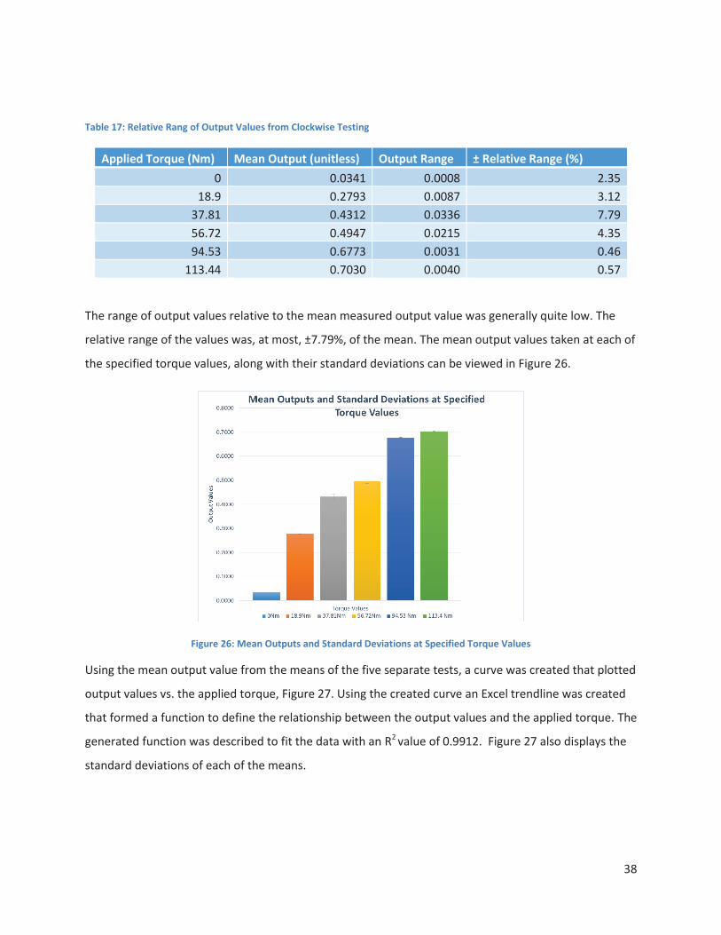
38
Table 17: Relative Rang of Output Values from Clockwise Testing
The range of output values relative to the mean measured output value was generally quite low. The
relative range of the values was, at most, ±7.79%, of the mean. The mean output values taken at each of
the specified torque values, along with their standard deviations can be viewed in Figure 26.
Figure 26: Mean Outputs and Standard Deviations at Specified Torque Values
Using the mean output value from the means of the five separate tests, a curve was created that plotted
output values vs. the applied torque, Figure 27. Using the created curve an Excel trendline was created
that formed a function to define the relationship between the output values and the applied torque. The
generated function was described to fit the data with an R2 value of 0.9912. Figure 27 also displays the
standard deviations of each of the means.
Applied Torque (Nm) Mean Output (unitless) Output Range ± Relative Range (%) 0 0.0341 0.0008 2.35
18.9 0.2793 0.0087 3.12 37.81 0.4312 0.0336 7.79 56.72 0.4947 0.0215 4.35 94.53 0.6773 0.0031 0.46
113.44 0.7030 0.0040 0.57

39
Figure 27: Calibration Curve for Torque Applied in the Clockwise Direction
The trendline generated equation that related output values to torque values is as follows:
Using this equation torque values were generated for each of the five tests performed at each known
torque value. The mean, maximum, and minimum torque values were then determined at each known
torque value. The relative range of these values was then determined by calculating the percent value of
the range in terms of the mean measured torque. The range represents the possible variation of
measured torque values to the mean measured torque value. The percent difference of the
measurements was then determined by calculating the percent value of the mean of the measured
torque to the known applied torque. These results can be viewed in Table 18.
Table 18: Percent Difference and Relative Rang of Torque Testing in the Clockwise Direction
Applied Torque (Nm)
Mean Measured Torque (Nm)
Maximum Measured Torque (Nm)
Minimum Measured Torque (Nm)
± Relative Range (%) ± Difference (%)
0 0.38 0.39 0.37 *3.33* *280.38* 18.9 17.33 17.74 16.67 6.14 8.31 37.81 40.97 45.60 39.15 15.73 8.36 56.72 53.82 55.90 51.26 8.62 5.11 94.53 100.58 101.13 100.20 0.92 6.40 113.44 108.31 108.85 107.62 1.13 4.52

40
As a note the percent relative range and difference for 0Nm torques was obtained by attributing the
known torque the value of 0.1Nm. Due to this low torque value the range of the percent difference and
relative range will be high. The range of the measured torque values, relative to the mean measured
values, were extremely different depending on the measured torque value. This indicates that the
results produced by the tester are highly variable between approximately 38 and 47 Nm of applied
torque. The percent difference between the known torque and applied torque were all under 10%,
however only the percent difference at 113 Nm was under 5%, meeting our performance constraints.
However, the lower relative ranges seen in the testing of the output values indicates that a better
defined calibration curve could produce better results. An enhanced calibration curve could be
produced through testing at more known torque values. Using an alternative program such as MATLAB
to produce the curve might also result in a better fit.
Due to the inherent offsets between the outputs produced by our system and strain, we adjusted our
output values to account for these offsets and graphed the true strain outputs verse the applied torque
values, Figure 28.
Figure 28: Correlation between Applied Torque and Strain
A trendline for this data was produced, which related the applied torque to the true strain, expressed in
milli-units. This trendline was found to fit the plotted data with an R2 value of 0.9939. The equation that
related torque to strain is as follows.
This equation would be useful for determining the strain experienced by the dynamometer during testing.

41
6.2 Calibration Testing for Counterclockwise Twist Release Testing The known release torques that were applied in counterclockwise testing were the same as those used
for clockwise testing. The same values were used because release torque values for clockwise and
counterclockwise release are theoretically the same for the same skier type.
6.2.1 Test setup and methods for counterclockwise twist release testing
The testing frames, pulleys, weights, and reference geometries used for clockwise testing were also used
for counterclockwise testing. The only difference between the two types of testing were that the
orientation of the testing frames and the direction in which the ropes attached to the lever arm were
reversed, so that torsion of the dynamometer occurred in the counterclockwise direction, as seen in
Figure 29.
Figure 29: Counterclockwise torque applicator pulley system
6.2.2 Calibration curve, results, and analysis for counterclockwise twist release testing
For initial counterclockwise testing, there were again five test runs at each of the specified torque
values, as well as at 0 Nm. Each of these individual tests were run for at least 10 seconds, which at a 1k
sampling rate, meant that there were at least 10,000 data points for each individual test. Within each
test run there were low standard deviations, which were dwarfed by the deviations seen between test
runs. These deviations were also not included for our calculations for percent difference and relative

42
range of the system. Between each test the system was disassembled and then reassembled to ensure
the robustness of the measurements.
The mean of the outputs of each of the five tests for each torque value was recorded. The maximum,
minimum, range, and mean values of these five mean output values were then calculated. The percent
relative range of the output was then determined by determining the percent value of the range in
terms of the mean output. The range represents the possible variation of output values to the mean
output value, which was used to create the calibration curve. The results of this analysis can be viewed
in Table 19.
Table 19: Relative range of output values from counterclockwise testing
Interestingly, the percent relative range of the output values has a much higher range for the
counterclockwise values, than the clockwise values. This could be due to the fact that the
counterclockwise outputs reduce to small values before becoming negative; so even though the range
of outputs from counterclockwise testing are smaller than those from clockwise testing, they account
for a larger difference in proportion to the size of the output values. This is corroborated by the fact that
the relative range of the 113 Nm measurement was much lower than at 57 and 95 Nm. The mean
output values taken at each of the specified torque values, along with their standard deviations can be
viewed in Figure 30.
Applied Torque (Nm) Mean Output (unitless) Output Range ± Relative Range (%)
0 0.1548 0.0047 3.02
18.9 0.0592 0.0003 0.49
37.81 0.0145 0.0003 2.24
56.72 0.0022 0.0006 29.50
94.53 -0.0387 0.0064 16.53
113.44 -0.0546 0.0012 2.11

43
Figure 30: Mean outputs and standard deviations at specified torque values applied in the counterclockwise direction
Using the mean output value from the means of the five separate tests, a curve was created that plotted
output values vs. the applied torque, Figure 31. Using the created curve an Excel trendline was created
that formed a function to define the relationship between the output values and the applied torque. The
generated function was described to fit the data with an R2 value of 0.99. This calibration curve fits the
majority of the data well, however, has a poor fit for low torque values. However, as we had determined
previously, we are most interested in the torque values that span from 37.81 Nm to 113.44 Nm, so
discrepancies in this portion of the curve are more allowable. Figure 31 also displays the standard
deviations of each of the means.
Figure 31: Calibration Curve for Torque Applied in the Counter Clockwise Direction

44
The trendline generated equation that related output values to torque values is as follows:
Using this equation torque values were generated for each of the five tests performed at each known
torque value. The mean, maximum, and minimum torque values were then determined at each known
torque value. The percent relative range of these values was then determined by calculating the percent
value of the range in terms of the mean measured torque. The range represents the possible variation of
measured torque values to the mean measured torque value. The percent difference of the
measurements was then determined by calculating the percent value of the mean of the measured
torque to the known applied torque. These results can be viewed in Table 20.
Table 20: Percent Difference and Relative Rang of Torque Measurements in the Counter Clockwise Direction
Applied Torque (Nm)
Mean Torque (Nm)
Maximum Torque (Nm)
Minimum Torque (Nm)
± Relative Range (%) ± Difference (%)
0 0.46 0.83 0.10 *159.18* *356.06*
18.9 15.84 15.91 15.77 0.87 16.17
37.81 43.85 43.97 43.72 0.57 15.98
56.72 53.87 54.15 53.60 1.01 5.02
94.53 94.32 96.15 89.03 7.56 0.23
113.44 113.06 113.85 112.43 1.25 0.34
Again, the percent relative range and difference for 0Nm torques was obtained by attributing the known
torque the value of 0.1Nm. Due to this low torque value the range of percent difference and relative
range will be high. The results of this testing reveal that the relative range of measured torque values,
compared to the mean values, was generally lower and more constant than the measured values in the
clockwise direction, with the majority of the values being under 2%. The percent difference between the
measured torque and applied torque was also lower than with clockwise measurements, with three of
the tested torque values being within 5% of the known applied torque. However, there were large
percent differences at the lower tested torque values, this can be explained by the poor fitting of the
trendline to the plotted data at lower torque values. This can be seen in figure 31 where output values
0.1548 through 0.0145 represent the torque values from 0 to 37.81 Nm. Due to this fact, an enhanced
calibration curve could result in measurements with much lower percent differences, especially in the
lower torque regions.

45
Due to the inherent offsets between the outputs produced by our system and strain, we adjusted our
output values to account for these offsets and graphed the true strain outputs verse the applied torque
values, Figure 32.
Figure 32: Correlation between strain and torque applied in the counterclockwise direction
A trendline for this data was produced, which related the applied torque to the true strain, expressed in
milli-units. This trendline was found to fit the plotted data with an R2 value of 0.966. The equation that
related torque to strain is as follows.
This equation would be useful for determining the strain experienced by the dynamometer during testing.
6.3 Calibration Testing for Forward Bending Release Testing Before conducting calibration testing, a range of torque values for testing was determined. To produce
an accurate calibration curve, many different points should be tested. Due to time constraints however,
we defined our calibration curve by testing done at six different known torques, including zero. These
values were determined from using anthropometric data combined with the ASTM standards for the
selection of release torque (CDC, 2010; ASTM, 2005). As this tester was designed for adult users, we felt
it was most important to have an accurate calibration curve in the range of release torque values used
by adult skiers. From our anthropometric data we determined that the 10th percentile female was 53.6
kg and from the ASTM release torque standards we established that this would encompass a type “I”
skier, who would have a release torque value of 141 Nm in forward lean release. We then established
that a 90th percentile male was 114.4kg, as the highest defined weight by the ASTM for release torque
selection is 95 kg, we decided that our highest torque value measured should be at least 452 Nm, which
was the release torque value for skier type “P” and the highest listed in forward lean release. However,

46
due to later concerns about the possibility of the extruded interface of the bottom piece deforming
under the higher loads, we determined to set our highest torque value measured to 297 Nm. This value
is slightly above that specified for skier type “M”, which encompasses skiers 95kg and greater, and is the
last skier type with an associated weight range. The torque values that our calibration curve was tested
with were thus 0, 118.88, 178.32, 237.75, and 297.19 Nm.
6.3.1 Test setup and methods for forward bending release testing
To apply the selected known torque values we created a pulley system that would connect to the top
end of our one meter long lever at an angle fifteen degrees below the horizontal. The decomposition for
the designed pulley system and calibration curve creation can be seen in Table 21.
Table 21: Create strain to torque calibration curve in forward bending release
Our pulley system for our clockwise calibration testing involved a simple wooden box frame constructed
with four 3”x3” pine columns, eight 2”x4” pine support boards, eight wood braces, and 24 3” wood
screws. The top 2”x4” support board of each frame had a stainless steel metal pulley, for use with 3/8”
diameter rope, with a 165 lb work load rating. The rope used for the pulley system was 3/8” diameter
polypropylene and mixed synthetic rope. Olympic weight(s) were again attached to the rope to apply
the known torque values. Due to the spacial constraints of our workspace and the Olympic weights that
were available to us, we chose to apply our bending loads via a pulley located fifteen degrees below the
horizontal plane of the point of the lever to which we attached the rope, a point 1.38m, 4’ 6”, from the
surface of the table we were testing on. To accomplish this, our pulley was located 1.22m, 4’, away from
the attachment point in the horizontal direction and 0.33m, 1.07’, away from the attachment point in
the vertical direction. A SolidWorks model of our testing setup, with important reference geometries,
can be viewed in Figure 33.

47
Figure 33: Forward bending torque applicator pulley system
The amount of weight needed for each side of the pulley system was calculated using the relationships
between pounds and kilograms, mass and force, and the equations:
where Mo was the moment at the center of the lever around which torque was applied, d was the distance of the applied force, 1.38m,
and was the angle between the lever arm and the force caused by the tension of the rope, 15°
Using this equation we found that 20, 30, 40, and 50 lb weights would be required to obtain the desired
amount of applied torque to the system. Table 22 shows the relationship between the mass applied to
the pulley system to the applied torque.
Table 22: The relationship between the applied mass and the applied torque
Mass (lbs)
Mass (kg)
Force (N)
Applied Torque (Nm)
20 9.09 89.18 118.88
30 13.64 133.77 178.32
40 18.18 178.36 237.75
50 22.73 222.95 297.19

48
6.3.2 Calibration curve, results, and analysis for forward bending release testing
Calibration testing was preformed five times at each of the specified torque values, as well as at 0 Nm.
Each of these individual tests were run for at least 10 seconds, which at a 1k sampling rate, meant that
there were at least 10,000 data points for each individual test. Within each test run there were low
standard deviations, which were dwarfed by the deviations seen between test runs, for this reason
these deviations were not included for our calculations for percent difference and relative range of the
system. Between each test the system was disassembled and then reassembled to ensure the
robustness of the measurements.
The mean of the outputs of each of the five tests for each torque value was recorded. The maximum,
minimum, range, and mean values of these five mean output values were then calculated. The percent
relative range of the output was then determined by determining the percent value of the range in
terms of the mean output. The range represents the possible variation of output values to the mean
output value, which was used to create the calibration curve. The results of this analysis can be viewed
in Table 23.
Table 23: Relative range of output values from forward bending testing
Applied Torque (Nm) Mean Output (unitless) Output Range ± Relative Range (%)
0 0.4877862 0.0009 0.18
118.88 0.654881 0.0015 0.23
178.32 0.695762 0.0012 0.18
237.75 0.7052584 0.0007 0.10
297.19 0.7129448 0.0010 0.14
The range of output values, relative to the mean measured outputs, was consistently much lower than
in both clockwise and counterclockwise testing, with all values being well under 1%. The mean output
values taken at each of the specified torque values, along with their standard deviations can be viewed
in Figure 34.

49
Figure 34: Mean outputs and standard deviations at specified forward bending torque values
Using the mean output value from the means of the five separate tests, a curve was created that plotted
output values vs. the applied torque, Figure 35. Using the created curve an Excel trendline was created
that formed a function to define the relationship between the output values and the applied torque. The
generated function was described to fit the data with an R2 value of 0.94. This calibration curve fits the
output values poorly compared to the other produced calibration curves. Figure 35 also displays the
standard deviations of each of the means.
Figure 35: Calibration curve for torque applied in the forward bending direction
The trendline generated equation that related output values to torque values is as follows:

50
Using this equation torque values were generated for each of the five tests performed at each known
torque value. The mean, maximum, and minimum torque values were then determined at each known
torque value. The relative range of these values was then determined by calculating the percent value of
the range in terms of the mean measured torque. The range represents the possible variation of
measured torque values to the mean measured torque value. The percent difference of the
measurements was then determined by calculating the percent value of the mean of the measured
torque to the known applied torque. These results can be viewed in Table 24.
Table 24: Percent Difference and Relative Range of Torque in the Forward Bending Direction
Applied Torque (Nm)
Mean Torque (Nm)
Maximum Torque (Nm)
Minimum Torque (Nm)
± Relative Range (%)
± Difference (%)
0 17.45 17.56 17.35 *1.18* *17347*
118.88 132.81 134.04 131.61 1.83 11.71
178.32 207.91 209.21 206.69 1.21 16.59
237.75 227.99 228.68 227.11 0.69 4.11
297.19 244.97 245.96 243.65 0.94 17.57
As in previous sections, the percent difference and relative range for 0Nm torques was obtained by
attributing the known torque the value of 0.1Nm. Due to this low torque value the percent difference
and relative range will be high. The results of this testing reveal that torque measurements within the
range of 0-297Nm would all have a range torque values that would be within ±2% of the measured
torque. This suggests that the tester would produce torque measurements with small amounts of
variance. The suspected reason that these results had a smaller range of torque values than those
attained for clockwise and counterclockwise testing, is that someone with professional experience with
applying strain gauges applied the strain gauges to the applicator tube we used for forward bending
testing. However, there was a consistently large difference between the measured and applied torque
values. This is due to the poor fit of the produced trendline to the plotted data, which can be seen in
figure 35. The only measured value which is within 10% of the applied torque, is the measured value at
238 Nm, which corresponds to an output value of 0.705. However, due to the repeatable nature of the
produced values and that the calibration curve was shown to poorly fit the produced data, an enhanced
calibration curve could result in lower percent differences at each of the measured values. However, a
second order polynomial may not be the best method of fitting this curve.

51
Due to the offsets between the outputs produced by our system and strain, we adjusted our output
values to account for these offsets and graphed the true strain outputs verse the applied torque values,
Figure 36.
Figure 36: Correlation between strain and torque applied in forward bending
A trendline for this data was produced, which related the applied torque to the true strain, expressed in
milli-units. This trendline was found to fit the plotted data with an R2 value of 0.9968. The equation that
related torque to strain is as follows.
This equation would be useful for determining the strain experienced by the dynamometer during testing.
6.4 SBB System Testing for Clockwise and Counterclockwise Release Testing After calibration curves were produced and initial testing for percent difference and relative range was
conducted on clockwise, counterclockwise, and forward bending applied loads, the device was tested in
a ski boot binding system. This testing was done to determine the percent difference and relative range
of our system under non-constant loading situations, specifically when used to release a ski boot from
its binding. The testing also served to provide information on the torque experienced by the binding
over time. The control “known” release torque values were taken from the release torque values taken
from Vermont Release Calibrator testing. However, there is some error associated with using the
Calibrator for our known release torque values as it is only guaranteed to be within ±5% of the actual
release torque, so for our experiment it would have a percent difference range of ±3.02 Nm of the mean
measured release torque value, approximately 60.45 Nm (ASTM, 2008).
The setup for our SBB system testing was the same for both clockwise and counterclockwise testing, the
only difference was the direction of the force applied to the lever arm. The SBB system was secured to

52
our testing station using a Tilt Vise from Vermont Ski Safety (Vermont Ski Safety, 2010). Two c-clamps
were used to connect the Tilt Vise to our testing surface was of the correct dimensions for direct vise
attachment. The Vermont Release Calibrator Prosthetic foot was used as the interface between the SBB
system and both testing devices. An explanation of how the Vermont Release Calibrator can be used can
be viewed in the State of the Art section of the paper. Figure 37 shows the testing setup for the Vermont
Release Calibrator tester, left, and for our electronic dynamometer tester, right. The blue markers seen
in the picture to the right are markers that we used to identify each strain gauge lead, to facilitate
correct connection of the leads to the full-Wheatstone bridge circuit.
Figure 37: Ski Boot Binding Testing Setup for the Vermont Release Calibrator (left) and the designed device (right)
For both clockwise and counterclockwise testing five tests were run with both the Vermont Release
Calibrator and our testing device. Testing with both devices was conducted until the boot released from
the binding. In regards to the designed tester, testing of release occurred over a period of approximately
4.2 to 8 seconds, which at a 1k sampling rate, meant that 4,200 to 8,000 data points were collected
during each test. Data acquisition through SignalExpress was also performed in the same manner for
these tests as it was for prior testing.
6.4.1 Clockwise testing results and analysis
Over a series of five test runs the Vermont Release Calibrator measured the mean release torque of the
SBB system to be 60.45 Nm, with four of the five release values being 60.5 Nm. These values can be
seen in Table 25. Subsequent testing of the same SBB system with our device produced a
characterization of all torque experienced by the tester during release over time. Due to this, our
produced data included a ramping section where torque was initially being applied and section between
when the binding was released and when we stopped the test. To account for these ramping and cut-off
sections the acquired data was only analyzed from the 2 to 4 second timeframe for their mean,
maximum, and minimum values for all tests. This was due to the fact that all of the tests evaluated were

53
at a stable state from 2 to four sections as seen by one example of the generated torque vs time graphs
in Figure 38. All of the generated torque vs time graphs can be viewed in Appendix F. However, as our
tests showed that the binding absorbed the load until an instantaneous release at a certain time-point,
we took the last non-zero, or near non-zero, torque value to be the release torque value, which
generally occurred after the 4 second mark. These values, as well as the range of torque values from 2 to
4 seconds can also be seen in Table 25. These values in combinations with the curves generated from
each test, Figure 38, serve to define the behavior of release.
Figure 38: Torque to release over time for clockwise run 1 with our device
Table 25: Characterization of torque to release measurements from a Vermont Release Calibrator and the designed device
These results suggest that the binding responds to the applied load by gradually displacing the boot
within the binding and then releasing instantaneously once the boot has reached a certain threshold of
displacement. This hypothesis would have to be corroborated with displacement testing in order to
0
20
40
60
80
0 2 4 6
Torq
ue
(Nm
)
Time (sec)
Clockwise Testing with SBB System Run 1
Run Number
Vermont Release Calibrator Measurement (Nm)
Maximum Torque (Nm)
Minimum Torque (Nm)
Mean Torque (Nm)
Torque at Release (Nm)
Torque Range (Nm)
1 60.5 62.214 55.88 58.956 57.94 6.331
2 60.5 61.536 59.010 60.281 60.80 2.526
3 60.5 61.539 59.009 60.269 61.13 2.530
4 60.25 61.538 59.011 60.259 61.53 2.527
5 60.5 61.538 59.012 60.264 59.93 2.527
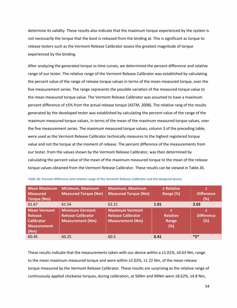
54
determine its validity. These results also indicate that the maximum torque experienced by the system is
not necessarily the torque that the boot is released from the binding at. This is significant as torque to
release testers such as the Vermont Release Calibrator assess the greatest magnitude of torque
experienced by the binding.
After analyzing the generated torque vs time curves, we determined the percent difference and relative
range of our tester. The relative range of the Vermont Release Calibrator was established by calculating
the percent value of the range of release torque values in terms of the mean measured torque, over the
five measurement series. The range represents the possible variation of the measured torque value to
the mean measured torque value. The Vermont Release Calibrator was assumed to have a maximum
percent difference of ±5% from the actual release torque (ASTM, 2008). The relative rang of the results
generated by the developed tester was established by calculating the percent value of the range of the
maximum measured torque values, in terms of the mean of the maximum measured torque values, over
the five measurement series. The maximum measured torque values, column 3 of the preceding table,
were used as the Vermont Release Calibrator technically measures to the highest registered torque
value and not the torque at the moment of release. The percent difference of the measurements from
our tester, from the values shown by the Vermont Release Calibrator, was then determined by
calculating the percent value of the mean of the maximum measured torque to the mean of the release
torque values obtained from the Vermont Release Calibrator. These results can be viewed in Table 26.
Table 26: Percent difference and relative range of the Vermont Release Calibrator and the designed device
These results indicate that the measurements taken with our device within a ±1.01%, ±0.63 Nm, range
to the mean maximum measured torque and were within ±2.02%, ±1.22 Nm, of the mean release
torque measured by the Vermont Release Calibrator. These results are surprising as the relative range of
continuously applied clockwise torques, during calibration, at 56Nm and 94Nm were ±8.62%, ±4.8 Nm,
Mean Maximum Measured Torque (Nm)
Minimum, Maximum Measured Torque (Nm)
Maximum, Maximum Measured Torque (Nm)
± Relative Range (%)
± Difference
(%)
61.67 61.54 62.21 1.01 2.02
Mean Vermont Release Calibrator Measurement (Nm)
Minimum Vermont Release Calibrator Measurement (Nm)
Maximum Vermont Release Calibrator Measurement (Nm)
± Relative Range
(%)
± Difference
(%)
60.45 60.25 60.5 0.41 *5*

55
and ±0.92%,±0.86 Nm, respectively, while the percent difference at these torque values were ±5.11%,
±2.86 Nm, and ±6.4%, ±6.02 Nm, respectively. Possible reasons why our results with the SBB system had
a smaller relative range and percent difference were that these tests were all conducted on the same
day, at the same time, unlike the calibration tests. Also, we did not remove the tester between each test
as we did with calibration testing. The tested torque value 60.4 Nm also lies between the two torques
values mentioned on the calibration curve, so the percent difference of the results is completely
dependent on the fit of the counterclockwise calibration curve at this value.
6.4.2 Counter clockwise testing results and analysis
Over a series of five test runs the Vermont Release Calibrator measured the mean release torque of the
SBB system to be 60.4 Nm. The values for these runs can be seen in Table 27. Subsequent testing of the
same SBB system with our device produced a characterization of all torque experienced by the tester
during release over time. Due to this, our produced data included a ramping section where torque was
initially being applied and section between when the binding was released and when we stopped the
test, which was the same as the behavior of the applied torque in the clockwise direction. To account for
these ramping and cut-off sections the acquired data was only analyzed from the 2 to 4 second
timeframe for their mean, maximum, and minimum values for all tests. This was due to the fact that all
of the tests evaluated were at a stable state from 2 to four sections as seen by one example of the
generated torque vs time graphs in Figure 39. All of the generated torque vs time graphs can be viewed
in Appendix G. However, as our tests showed that the binding absorbed the load until an instantaneous
release at a certain time-point, we took the last non-zero, or near non-zero, torque value to be the
release torque value, which generally occurred after the 4 second mark. This procedure was the same as
that used for the characterization of the torque vs time data from clockwise testing. These values, as
well as the range of torque values from 2 to 4 seconds can also be seen in Table 27. These values in
combinations with the curves generated from each test, Figure 39, serve to define the behavior of
release.

56
Figure 39: Torque to release over time for counterclockwise run 1 with our device
Table 27: Characterization of torque to release measurements from a Vermont Release Calibrator and the designed device
Run Number
Vermont Release Calibrator Measurement (Nm)
Maximum Torque (Nm)
Minimum Torque (Nm)
Mean Torque (Nm)
Torque at Release (Nm)
Torque Range (Nm)
1 60.25 61.996 58.960 60.474 61.43 3.036
2 60.5 61.995 58.959 60.501 60.98 3.035
3 60.5 61.996 58.963 60.472 60.28 3.033
4 60.5 61.997 58.960 60.466 61.65 3.037
5 60.25 61.993 58.959 60.468 61.62 3.034
These results corroborate the response patterns we identified in clockwise release; that the binding
responds to the applied load by gradually displacing the boot within the binding and then releasing
instantaneously once the boot has reached a certain threshold of displacement. This hypothesis would
have to be corroborated with displacement testing in order to determine its validity. The maximum
torque experienced by the system was also not the same value as the torque that the boot is released
from the binding at.
After analyzing the generated torque vs time curves, we determined the percent difference of the
values measured from our tester from the values measured with the Vermont Release Calibrator and
relative range of the values measured from our tester. The percent difference and relative range of the
Vermont Calibrator measurements and of our designed device were assessed in the same manner as
they were for clockwise testing. The relative range of the Vermont Release Calibrator was established by
calculating the percent value of the range of release torque values in terms of the mean measured
torque, over the five measurement series. The range represents the possible variation of the measured
0
20
40
60
80
0 2 4 6 8 10To
rqu
e(N
m)
Time (sec)
Counterclockwise Testing with SBB System Run 1

57
torque value to the mean measured torque value. The Vermont Release Calibrator was assumed to have
a maximum percent difference of ±5% from the actual release torque (ASTM, 2008). The relative rang of
the results generated by the developed tester was established by calculating the percent value of the
range of the maximum measured torque values, in terms of the mean of the maximum measured torque
values, over the five measurement series. The maximum measured torque values, column 3 of the
preceding table, were used as the Vermont Release Calibrator technically measures to the highest
registered torque value and not the torque at the moment of release. The percent difference of the
measurements from our tester, from the values shown by the Vermont Release Calibrator, was then
determined by calculating the percent value of the mean of the maximum measured torque to the mean
of the release torque values obtained from the Vermont Release Calibrator. These results can be viewed
in Table 28.
Table 28: Percent difference and relative range of the Vermont Release Calibrator and the designed device
These results indicate that the measurements taken with our device had a range of ±0.007%, ±0.004
Nm, in respect to the mean maximum measured torque and were within ±2.64%, ± 1.6 Nm, of the mean
release torque measured by the Vermont Release Calibrator, 60.4 Nm. These results are surprising as
the relative range of continuously applied counterclockwise torques at 56Nm and 94Nm were ±1.01%,
±0.56 Nm, and ±7.56%, ±7.1 Nm, respectively, while the percent difference from the known applied
torque at these values were ±5.02%, ±2.91 Nm, and ±0.23%, ±0.22 Nm, respectively. Possible reasons
why our results with the SBB system were more accurate and reproducible were that these tests were
all conducted on the same day, at the same time, unlike the calibration tests. Also, we did not remove
the tester between each test as we did with calibration testing. The tested torque value 60.4 Nm also
lies between the two torques values mentioned on the calibration curve, so the percent difference of
Mean Maximum Measured Torque (Nm)
Minimum Maximum Measured Torque (Nm)
Maximum Maximum Measured Torque (Nm)
± Relative Range (%)
± Difference
(%)
61.995 61.993 61.997 0.007 2.64
Mean Vermont Release Calibrator Measurement (Nm)
Minimum Vermont Release Calibrator Measurement (Nm)
Maximum Vermont Release Calibrator Measurement (Nm)
± Relative Range
(%)
± Difference
(%)
60.4 60.25 60.5 0.414 *5*

58
the results from the known value is completely dependent on the fit of the counterclockwise calibration
curve at this value.
6.5 Additional Calibration Curve Validation Testing for Forward Bending
Testing Additional validation of the calibration curve for forward bending testing was done instead of testing
with the SBB system. This was due to the fact that the calibration curve for bending was shown have
high percent differences, between ± 4.11% and ± 17.57%, over the range of tested values. Additionally,
the Vermont Release Calibrator would not stay in the test boot during attempts at forward bending
release, as the tongue of the tested boot would displace and come out. It was later determined that for
this mode of release testing, a strap is placed under the heel of the boot. This strap allows for the
upward load to be transmitted. Validation of the calibration curve for forward bending was carried out
using the same test methods used for creating the calibration curve and testing the measured torque
values against the known applied torque values in forward bending. However, for these tests we
evaluated the percent difference and relative range of the measured torque values generated by the
device outputs and calibration equation at a known torque value of 148.6 Nm. Using the equation,
where Mo was the moment at the center of the lever around which torque was applied, d was the distance of the applied force, 1.38m,
and was the angle between the lever arm and the force caused by the tension of the rope, 15°
from section 6.3.1 we determined that a load of 25 lbs would be needed to generate a torque of this
magnitude.
6.5.1 Testing results and analysis
Calibration testing was preformed five times at 148.6Nm, with each of these individual tests being run
for at least 10 seconds, which at a 1k sampling rate, meant that there were at least 10,000 data points
for each individual test. Within each test run there were low standard deviations, which were dwarfed
by the deviations seen between test runs, for this reason these deviations were not included for our
calculations for percent difference and relative range of the system. Between each test the system was
disassembled and then reassembled to ensure the robustness of the measurements. This procedure was
the same used as the procedure used for initial calibration curve testing.
The same trendline generated equation, derived in section 6.3.2, that related output values to torque,
for calibration testing was used for the validation testing:

59
Using this equation torque values were generated for each of the five tests performed at each known
torque value. The mean, maximum, and minimum torque values were then determined at each known
torque value. The relative range of these values was then determined by calculating the percent value of
the range in terms of the mean measured torque. The range represents the possible variation of
measured torque values to the mean measured torque value. The percent difference of the
measurements was then determined by calculating the percent value of the mean of the measured
torque to the known applied torque. These results can be viewed in Table 29.
Table 29: Percent difference and relative range of the forward bending calibration curve at 148.6 Nm of applied torque
These results further demonstrate the unreliability of the torque values generated by our device with
torque applied in forward bending. The difference of the measurements from the applied 148.6 Nm was
within ±12.57%, ±18.68 Nm, which is a reflection of the poorly defined calibration curve. The relative
range of the measured values, ±2.66%, ±4.49 Nm, was also greater than from the initial calibration
testing, where the worst percent relative range was 1.83%, ±2.17 Nm. This leads to concerns about the
consistency of our device and suggests that further testing is needed.
7. Design Iteration Torque to release may be insufficient to identify injurious situations from non-injurious situations, as is
the case with the “bow effect” [Appendix A] (Brown and Ettlinger, 1985; Young, 1989). An electronic
torque tester interfaced with a displacement sensor provides several advantages. A torque-
displacement binding test system has the ability to test for both torque-to-release and work-to-release.
Measuring work-to-release will identify a bindings shock absorptive capabilities and thus its
susceptibility for inadvertent releases caused by such mechanisms as the “bow effect”.
Run Number
Mean Measured Torque (Nm)
Maximum Measured Torque (Nm)
Minimum Measured Torque (Nm)
± Relative Range (%)
± Difference (%)
1 168.66 169.95 167.96 2.66 12.57
2 168.01 168.95 166.97
3 167.23 167.96 166.48
4 166.55 167.47 165.98
5 165.96 166.48 165.49

60
A displacement sensor for this system must meet previously established constraints of the project;
sensor uncertainty must be within ±0.2 mm and remain within the project budget. Uncertainty was
defined using the standards described in ASTM E2655, which defines uncertainty as “an indication of the
magnitude of error associated with a value that takes into account both systematic errors and random
errors associated with the measurement or test process” (ASTM E2655, 2008). The equation for
uncertainty from ASTM E2655 is as follows:
Uncertainty=
Where σ= the standard deviation, and n= the number of measurements
n= the number of measurements x= the sample = the sample mean
Several sensor options were considered during preliminary research [Table 30]. The parameters
compared between the sensor options were measurement method, uncertainty, and cost.
Table 30: Displacement sensor comparison

61
Initial design requirements were defined using Nam Suh’s axiomatic design theory [Appendix B], and
fundamental requirements and design parameters of the system were defined in Acclaro software. The
utmost fundamental requirement of this displacement sensor system is the ability to measure angular
displacement of the boot in binding during several loading conditions [Table 31]
Table 31: Initial decomposition for torque-displacement binding tester
7.1 Optical Mouse Recent work at Worcester Polytechnic Institute was completed titled ‘Torque-Displacement Binding
Tester’ by (Merrill, 2013). In this project feasibility testing was performed using an optical mouse as a
displacement sensor. ‘The optical mouse as a two-dimensional displacement sensor’ also validates a
mouse for x-y displacement measurement (Ng, 2003). Testing included linearity, repeatability, and
uncertainty. At roughly $20, a mouse was an affordable sensor. Electronic integration was easily
performed using readily available National Instruments software. Considering the aforementioned, the
initial displacement system design utilized an optical mouse as the sensor.
7.1.1 Design Decomposition
First, a design decomposition was created to determine how the mouse would be used to obtain
accurate data over time [Table 32].

62
Table 32: Decomposition for a displacement measurement system utilizing an optical mouse
In order to measure displacement of the boot accurately, simultaneous and stiff articulation of the
mouse is necessary. To satisfy this requirement a ‘detachable and stiff fixation arm’ would grapple the
mouse on the side of the boot. This arm would articulate the mouse with any boot displacement. Due
to the several loading conditions during test, a detachable and adjustable solution is required. In order
to connect the arm and mouse, a spring loaded pin would be used to ensure precise z-axis distance. An
optical mouse is inoperable without a proper surface to image from. The arm/mouse must also be
secured to the ski boot. To accomplish this, a pair of brackets would locate a rod along the length of the
side of the boot. The arm would then secure to this rod using a shaft collar. This would complete the
physical design. For twist release only x-y position is considered, and only x-z position is considered for
bending.
Measuring displacement also requires the ability to read and export displacement data electronically.
To satisfy this requirement we utilized the virtual instrument capabilities of National Instruments
Labview software. As the mouse travels across the computer screen during binding release, the x-y
location of the mouse and time data is exported to Excel for analysis. With this decomposition, a fully
exhausted and mutually exclusive design is accomplished.
7.1.2 Shortcomings of Optical Mouse
Despite the findings of other scholarly works, testing was performed to fully validate linearity,
repeatability and uncertainty within the scope of our design. Despite exhaustive experimentation
(Appendix H), the level of uncertainty of an electronic mouse was not within our constraint of 0.2 mm.
Despite a rated resolution of 2000 dpi, an optical mouse is not a viable sensor in this application.
Several sources of error were analyzed and documented.
63
Firstly, an optical mouse’s accuracy is strictly dependent on a precise z-axis distance. With any
separation from the imaging surface, the mouse becomes inoperable. In binding testing procedures the
boot may twist and roll along the x-axis creating z-axis separation. This is difficult to mitigate in a
binding test. A third source of error with a mouse is top speed. Binding testing is to be performed with
applied torque for a maximum of 5 seconds (ASTM, 2009). This quick release may be difficult to capture
with an electronic mouse, a 1000 dpi gaming mouse has a top speed around 0.5 m/s (Windows, 2002).
This is not adequate for this application.
Additional error can be incurred due to smoothing or anti-aliasing functions built in to the mouse
hardware. Designed to smooth the translation of the cursor on the screen, these minor adjustments can
affect trajectory across the screen as well as cause significant lag. These properties will dramatically
decrease the accuracy of a computer mouse. Lastly, screen size will limit the amount of recordable
displacement distance. If the cursor runs into the edge of the screen during testing, data is halted at
that point. This limitation requires additional preliminary setup, and may go unnoticed.
7.2 NDI Polaris A highly accurate spatial measurement system, the Northern Digital Polaris, was developed to further
image-guided surgery in operating rooms. Using advanced tracking algorithms this system provides
exceptional accuracy, a 95% confidence interval of 0.4 mm (Wiles et al., 2004). Producing a large virtual
measurement volume [Figure 40], both passive and active markers can be tracked within the working
space. Active markers produce infrared light that are activated by an electrical signal, while passive
markers use retro-reflective coatings to reflect infrared light back to the sensor. The price of such a
system is in upwards of $1500, making this an unmarketable solution. Despite this price tag, further
testing was performed in order to understand the technology and the potential for this application. This
portable solution was provided by the Worcester Polytechnic Institute ‘Automation and Interventional
Medicine Laboratory’, providing the means to analyze image tracking hardware for this application.

64
Figure 40: Volume of Polaris measurement range (NDI, 2014)
2.2.1 Design Decomposition
The following decomposition demonstrates how the NDI Polaris would be used to obtain accurate
displacement data [Table 33].
Table 33: Decomposition for a displacement measuring system utilizing the NDI Polaris
The NDI Polaris can reproduce a transformation of movement using 3D Euclidean positioning data (Wiles
et al., 2004). In order to obtain necessary data, the boot’s position is tracked with respect to a reference
position. This reference was located directly along the x-axis with a passive marker. As the boot moves
during testing, this motion is also tracked with a second passive marker. Comparing the initial to the
final position yields a complete transformation of displacement. For twist release only x-y position is
considered, and only x-z position is considered for bending.
The Polaris system also has the capability to electronically read and export data to Excel. This feature
produces 3D Euler angle point per frame. This complete data set can be ignored, only focusing on the
necessary axis transformations.

65
7.2.2 Shortcomings of NDI Polaris
Validation testing was performed with the Polaris device in an attempt to validate its use as a
displacement sensor. A simple displacement test was conducted in attempt to obtain data regarding
the linearity, repeatability and accuracy of the system (Appendix I). Despite several tests, results were
unfavorable. With a nominal uncertainty of 0.4mm, data estimated an additional error magnitude of
0.3mm (NDI, 2014; Wiles et al., 2004). Based on the required accuracy of ASTM standard testing
procedures, this tool does not meet constraints. These series of experiments did however provide
excellent insight into imaging technology for tracking purposes.
Several other shortcomings were recognized through experimentation. Firstly, the working space
required by the Polaris is quite large. Nearly a 10’x10’ testing area is required. This requirement is not
ideal in local ski shops where space is a premium. Another difficulty with this device is with its
integration with a torque-to-release tester. Polaris data can be exported to Excel as a running series of
frames and associated 6D position. No time stamp data is included however, increasing difficulty of
aligning the two peaks of torque and displacement data. The cost of the equipment must also be
considered. With a price tag of greater than $1,000, this does not meet project constraints set
previously. Overall the NDI Polaris is not a viable displacement sensor for this application.
7.3 Additional Displacement Sensors Following difficulty with the Mouse and the NDI Polaris, several other displacement sensor options were
explored. Inadequacies of these two systems were recognized and improved upon. A major necessity
was the level uncertainty. Constraints requiring uncertainty of 0.2mm require a highly accurate, and
therefore more expensive, sensor. The required space for such a sensor was also a concern. Ideally a
working space would a table top. With an electronic torque-displacement sensor, access to a computer
is vital. Budgetary constraints were also considered.
7.3.1 Rotary and String Potentiometers
Rotary potentiometers express angular rotation in terms of voltage output. These highly accurate
devices are sensitive to within 0.1mm, sufficient for this application. They can be used to measure both
linear and angular displacement and can be easily integrated with a torque-to-release tester. Rotary
potentiometers can also be spring loaded, called a string potentiometer. By attaching two of these
spring loaded string pots can be attached to the boot, measuring both x and y axis displacement [Figure
41]. The potentiometer on the toe of the boot measures x position, and the side mounted pot measures
position on the y axis. The following equation can then be used to calculate displacement:

66
√
Where
With a stroke length of over 200mm, this is adequate capability for expected boot-binding displacement.
The price of these sensors can be upwards of $300 for a pair. This is a direct result of its high precision
and repeatability capabilities. Despite this somewhat high cost, expected results are much better with
these sensors. This is a potentially viable option for a torque-displacement tester.
Figure 41: Displacement measurement with string potentiometers
7.3.2 Rotary Encoders
Another sensor to be considered is rotary encoders. These devices measure displacement by converting
angular position to analog or digital code. There are two main types of rotary encoders: incremental
and absolute. Absolute rotary encoders Incremental rotary encoders maintain position information
when power is removed. Incremental encoder records changes in position, but does not initiate with a
fixed relation to physical position. The capability to “zero” the sensor with its initial position, make

67
incremental encoders the better choice for this application. With a precision up to 2/1000 of a
millimeter and a cost of $100 per encoder, rotary encoders are promising. Designing a displacement
system with these sensors is more difficult however. Typically, rotary encoders are shaft driven, a
motion not easily captured over two axes. Setup is similar to string potentiometers, using a tether to
turn the shaft of the encoder. Highly precise and affordable, rotary encoders are a viable option for this
application. Additional design time would yield an effective displacement tool (BEI Sensors, 2014).
7.3.3 Leap Motion
Another possibly effective tool for measuring displacement is the Leap Motion. This new product is
used to translate hand and finger motion and translate the motion electronically, analogous to a mouse.
This system requires no touching or contact and manipulation is responsive to all ten fingers at once.
Three infrared LEDs and two IR cameras create a 6 cubic foot workspace [Figure 42]. Analyzing 300
frames per second, information is sent through USB to the computer (LeapMotion, 2014).
Figure 42: Working range of a LeapMotion (LeapMotion, 2014)
The Leap Motion is listed with a precision of 1/100th of a millimeter (LeapMotion, 2014). With a cost of
only $80, the specifications are extremely impressive. However, this is a new technology. As a venture
backed project, applications for the device are broad. Currently the system is only capable of reading
hand motion. That being said, Leap Motion provides developer resources regarding the device API. This
access provides application development. In order to measure ski boot displacement, the system must
be able to track a marker on the boot. With someone who is knowledgeable of Computer Science there
is a great opportunity for precise image tracking. This small device is an excellent candidate for a
torque-displacement system.

68
8. Discussion
8.1 Satisfaction of the Objective The objective of this Major Qualifying Project was to design an alpine ski binding testing device that
measures the torque, displacement, and work to release ski boots from bindings in response to multiple
quasi-static loading configurations in the y and z axis. Such a test device would be able to identify ski
binding devices’ susceptibility for inadvertent release [Appendix A].
This objective was partially satisfied with the successful design and manufacture of an electronic torque
dynamometer. Several tests were performed in clockwise, counter-clockwise, and forward bending
loading configurations, y and z axes, respectively. A torque-to-release calibration curve was calculated
for each direction of testing by plotting the output of our tester against known applied torque values
and creating a second order polynomial trendline using the least squares method in Excel. The
equations that defined these trendlines were used to determine an unknown applied torque.
Due to ineffectual displacement sensors, work-to-release was not measured. Several additional options
were explored and described regarding the feasibility for successful system integration; the Polaris
Optical Tracker, rotary encoders, string potentiometers, and Leap Motion optical controller.
8.1 Results and Satisfaction of Constraints The satisfaction of project constraints are shown in Table 34 below.
Table 34: Satisfaction of project constraints
Constraint
Final Design
Success
Constraints for Calibration Testing
Based on ASTM Standards:
Torque testing must be no greater than ±5% of the known applied torque during calibration testing, using the equation from ASM F1062, in the Z-axis.
±16.2% No
Torque testing must be no greater than ±5% of the known applied torque during calibration testing, using the equation from ASM F1062, in the Y-axis.
±17.6% No
Constraints for Testing with a Ski
Boot Binding System Based on ASTM
Standards:
Torque testing must be no greater than ±5% of the release torque determined through testing with a Vermont Release Calibrator,
using the equation from ASTM F1062, in the Z-axis. ±2.64% Yes
Torque testing must be no greater than ±5% of the release torque determined through testing with a Vermont Release Calibrator,
using the equation from ASTM F1062, in the Y-axis. N/A No
Additional Constraints:
The device must be compatible with existing ski boot binding setups. Yes Yes
Displacement testing must be accurate within 0.2 mm (ASTM, 2009; ISO, 2009). 0.45mm No
Customer cost must be under $350. $350 Yes
Design prototype must be under $500. $500 Yes

69
The range of measurements indicated that our measured torque values had a higher degree of
variability in both modes of twist testing than in bending testing. Initial torque testing revealed that the
greatest difference, in percent, between known and applied torques in the clockwise direction was
±8.4% of 38 Nm, or ±3.2 Nm. The greatest difference in the counterclockwise direction was ±16.2% of
18.9 Nm, or 3.06 Nm. While the greatest difference in the forward bending direction was ±17.6% of 297
Nm, or 52.2 Nm. The percent difference between the known torque and the measured torque is
displayed as a percentage of the magnitude. This percentage was determined as a result of the
calculated calibration curve. This calibration curve was calculated using six data points in the twist
directions and five data points in bending testing. Overall results could be improved by creating a better
defined calibration curve through testing at more reference points. This will dramatically increase the
likelihood of satisfying the first two constraints.
The percent difference between the applied torque and the known torque during ski boot-binding
testing met specified constraints about the z-axis. Clockwise testing revealed a 2.02% difference in
magnitude between the Vermont Release Calibrator value and the calculated data, while counter
clockwise measurement resulted in a 2.64% difference. The constraints that we developed based on
ASTM standards require that these measurements must be no greater than ±5% of the release torque
measured with the Vermont Release Calibrator, therefore this constraint is met. However, these results
were far superior than those obtained in calibration testing, which suggests that further testing should
be conducted to verify these results.
Continued validation of the calibration curve for forward bending testing was done instead of testing
with the SBB system. This was due to the fact that the calibration curve for bending was shown to be
highly inaccurate, between ± 4.11% and ± 17.57%, over the range of tested values and the fact that the
Vermont Release Calibrator would not stay in the test boot during attempts at forward bending release,
as the tongue of the tested boot created major sources of error. These results further demonstrate the
unreliability of the torque values generated by our device with torque applied in forward bending. The
difference of the measurements from the applied 148.6 Nm was within ±12.57%, ±18.68 Nm, which is a
reflection of the poorly defined calibration curve. The relative range of the measured values, ±2.66%,
±4.49 Nm, was also greater than from the initial calibration testing, where the worst percent relative
range was 1.83%, ±2.17 Nm. This leads to concerns about the consistency of our device and suggests
that further testing is needed.

70
This system was designed under compatibility requirements for existing adult ski boot binding
technology. All makes and models of adult ski-boot-binding systems can be tested using the prototype
dynamometer as it interfaces with the universal Vermont Release Calibrator prosthetic foot.
Displacement sensor results were inadequate, as the measured uncertainty for both the NDI Polaris and
optical mice were greater than ±0.2mm. The mouse was determined to have an uncertainty of
±0.68mm. The NDI Polaris system is listed with a nominal precision of 0.4mm, and an error of ±1.6mm
was calculated when using the system to track the position of a ski boot.
Throughout the design and implementation process the prototype and projected consumer costs were
documented and an effort was made to keep both costs within their respective constraints. We met the
$500 prototype constraint easily, as most of the necessary components and software required were
provided by the school. We also avoided manufacturing costs by machining the required pieces
ourselves. Our final prototype costs were $61.49 excluding tax and shipping fees. Tax and shipping fees
were mitigated by ordering all circuit components from DigiKey and all stock material from McMaster-
Carr. The projected consumer cost was much higher than our initial prototype cost as the consumer
would have to pay for the National Instruments DAQ, which is $189, and for machining. Under the
assumption that our device would take two hours to machine, we projected manufacturing costs to be
$50. However, the software needed for using our device, Labview SignalExpress, as well the necessary
NI-MAX drivers can be downloaded for free from the National Instruments Website (National
Instruments, 2014). The final consumer cost for our device was $338.56, not including the Vermont
Release Calibrator Prosthetic Foot, which costs $200 (Vermont Ski Safety, 2010). The cost of the
prosthetic foot was ignored when assessing the satisfaction of our constraint due to the prevalence of
the Vermont Release Tester among ski shops and teams. Tables that document the cost of each
component and the amount spent, excluding tax and shipping fees, can be seen in Appendix J.
8.3 Impact of Solution The existing torque to release testers have no way to interface with future displacement to release
measurements. Although we were unable to create a work to release testing device, we were able to
create an electronic testing device that measures the applied torque to the ski-boot-binding system over
time, which would be able to interface with later displacement measuring devices. The target market is
ski shops and ski racers who wish to mitigate inadvertent binding release. Providing the ability to
further differentiate between effective and ineffective bindings, through work to release testing, is

71
pivotal in preventing associated injuries. Successful, design, development and testing of such a device
would create a new technology that would advance the safety of skiing.
Using stock parts, simple CAD models and machining processes, the developed electronic torque tester
could easily be duplicated. Due to the designs low cost, weight, and size it provides a viable option for
both large and small ski shops, as well as the individual ski racer.
8.4 Future Recommendations Despite our design’s ability to measure torque applied to a ski-boot-binding system multiple
improvements could be made to the design. The top and bottom pieces could be machined out of a
material with a higher elastic modulus as the bottom piece of the design can currently only withstand a
maximum load of 297 Nm without plastic deformation. By machining both pieces out of the same higher
elastic modulus stock, only one type of 2 inch diameter stock would have to be purchased.
In future designs work to release could be incorporated through developing a displacement measuring
system. This system would have to have an analogue or digital output that could be measured with the
portable NI DAQ to produce displacement measurements over time. This would allow for direct
correlation between the torque and displacement measurements. The uncertainty of the displacement
sensors would have to be within ±0.2 mm, without being exorbitantly expensive. To this end the string
potentiometers and LeapMotion controller are potentially viable future options.
9. Conclusions The initial main objective of this MQP was to design an alpine ski binding tester that could measure the
simultaneous torque and displacement experienced by a ski boot-binding system under quasi-static
loading conditions. This would allow for the identification of the work required to release a ski boot
from its binding. The greater the evaluated binding’s measured work to release, the greater its ability to
prevent inadvertent release at large, instantaneously applied loads. However, due to the tested
displacement sensors having an unacceptably high uncertainty of ±0.68mm or greater, and additional
restrictions that made them unsuitable options for use with a ski boot-binding system, a work-to-release
device was not created. However, an electronic torque to release dynamometer that could be
integrated with several identified possible future displacement methods, was designed, manufactured,
and tested.

72
Design Accomplishments:
The design was able to measure applied torque over time under constant loading situations and
when used to measure the torque to release a ski boot from a binding
The design could be integrated with future displacement measuring devices
The design could be reproduced for approximately $339 by ski shops or ski teams
Assessment of the effectiveness of the design method:
Allowed for the design of a modular device where functional requirements of the system were
addressed through separate design parameters
The design of the device allowed for easy identification of malfunction within the separate
components. If a function of the device was not operational, the specific design parameter that
accomplished that functional requirement could be easily identified and repaired.
Remaining Issues:
The device was unable to measure torque within ±5% of the known applied torque in clockwise,
counterclockwise, or forward bending during initial calibration testing.
The measured torque values produced by the device under forward bending loads had a larger
percent difference from the known applied torques than in clockwise and counterclockwise
loading configurations. These differences constituted up to 17.57% of the applied torque, or
52.2 Nm.
The torque measurements could be improved through improving the fit of the produced
calibration curve. The calibration curves relating output strain measurements and applied
torque could be improved through evaluating the strain outputs at more known applied
torques.
The bottom piece of the device would deform under loads over 297 Nm in forward bending,
which could be addressed by re-machining the top and bottom pieces out of a higher modulus
material.
Strain gauges are highly temperature dependent; the torque values measured by the device
could vary under large variations in temperature.

73
The robustness of the design should be continued to be tested. The calibration curves used to
compare output strain to known applied torque values should be replicated to test the systems
reproducibility over time.
Displacement measurement options such as the LeapMotion and string potentiometers should
be continued to be assessed for future incorporation with the design.

74
Appendix A: Causes and Effects of Inadvertent Release
Inadvertent release is often caused by inappropriate retention; the inability of the binding to retain the
boots to the ski during normal skiing maneuvers (Ettlinger et al., 2009). This can be caused by a number
of mechanisms including hardware problems and bad skiing practice coupled with under defined heel
release mechanisms. Hardware problems include sluggish or faulty forward pressure mechanisms in the
toe or heel piece. A flaw in either of these mechanisms will cause a gap to form between the boot and
binding. This allows the boot to escape from either the toe or heel piece, depending on the situation,
without opening of the heel piece (Ettlinger, 2010). Ettlinger also describes a method of release that
usually happens to less experienced skiers moving at a slower speed, and in heavier snow, called the
“superman effect”. In the superman effect the skier applies a torque through forced clockwise and
counterclockwise motions of the lower leg, setting off the twist release mechanism in the toe piece.
Another method of inadvertent release, “the bow effect” [Figure 9] is caused by both skier error and the
under design of the heel piece. The typical mechanism for the bow effect is when a forward leaning skier
presses the shovel of his ski into a depression, loading the tip of the ski, causing the heelpiece to release
(Brown and Ettlinger, 1985; Ettlinger, 2010, Young, 1989). This type of release is recognizable by the
rearward trajectory of the released ski, caused by the
forces acting on the shovel of the ski. In the bow effect
the heelpiece releases at a much lower bending moment
because it can only sense vertical forces. In 1985 Brown
and Ettlinger completed testing to evaluate retention
characteristics part of which included reproducing the
bow effect using an alteration of Test 2.5 in ASTM Method
F 504-77. Using this test method they found that they
could reduce the bending moment at which heel release
occurred from 240 Nm to 120 Nm, without adjusting the binding settings. In a correlating study about
elevated binding settings in alpine racers, Young found that bow releases had occurred despite the heel
settings often being for or five, in one instance ten, above ASTM recommendations for expert fast skiers.
This is especially dangerous because the heel piece will release seemingly regardless of the release
setting.
Figure 43: "Bow Effect" Inadvertent Release (Brown and Ettlinger, 1985)

75
Skiers who experience the bow effect, or other retention related
inadvertent releases, often blame the pre-release on the release
torque settings of the binding, which leads to a phenomenon called
the “ratchet effect” (Ettlinger, 2010). This is when expert skiers, who
already have the highest release torque setting standards per ASTM F
939-05a, continue to raise the release torque levels on their bindings
in order to avoid inadvertent releases. In the case of the bow effect,
faulty forward pressure mechanisms, or other types of retention
related issues, raising the release torque is not going to stop inadvertent release. However, raising the
release torque beyond the standards increases the chance of binding release failure under high loading
situations, and subsequent lower leg damage. A severe demonstration of this was when Matthias
Lanzinger’s left ski failed to release after a crash in a World Cup Super-G run in 2008 [Figure 10], the
crash was so severe that it led to his leg being amputated (New York Times, 2008; Merrill, 2013).
Although the release settings defined by ASTM F 939-05a have helped reduce lower leg injuries and
overall injuries by 80-90% over the last thirty years, there are still some problems with binding release
accuracy in regards to the heel piece (Beynnon et al., 1997;
Paletta et al., 1994). This largely because the bending
moment sensed by the leg does not always agree with the
moment sensed by the binding [Figure 11] (Brown et al.,
1985). The moment sensed by binding (MB) is the vector
product of the force on the ski and the distance between this
force and the bending fulcrum, r. However, the moment
experienced by the leg (ML) is the product of the force and
distance of that force from the center of the distributed load on the tibia, R. As the r displacement
remains constant, a skiers’ ability to change the R displacement through forward lean, coupled with a
small deceleration force on the shovel of the ski can cause the binding to release at a much higher
moment than desired. However, a large deceleration force at the shovel of the ski in these same
conditions can cause inadvertent release. Though ASTM F504-05 testing methods, 2.3 and 2.5, have
been developed to test for these issues, they have not been able to demonstrate most retention issues
(ASTM, 2005).
Figure 44: Failure of Ski to Release
Figure 45: Bending Moment Sensed by the Binding vs. the Tibia (Brown and Ettlinger, 1985)

76
Appendix B: Axiomatic Design Concepts
Nam Suh’s Axiomatic Design method was utilized to decrease design time and increase efficacy. To do
this the designer first determines the designs objectives by defining them in terms of specific
requirements known as functional requirements (FRs)
(Suh, 1990). To satisfy these functional requirements
solutions, design parameters (DPs), of the physical
domain, must be generated. FRs and DPs are naturally
organized into a hierarchal structure from which they
can be decomposed; the first level FRs are the most
fundamental of a design. To develop the FR and DP
hierarchies the designer has to travel back and forth
between the functional and physical domains of the FRs
and DPs [Figure 12]. After completing first level FRs first level DPs have to be established in order to
identify the next level of FRs. The alternating pattern helps to streamline decomposition by allowing the
designer to look at fewer FRs, or objectives, at a time. This reduces the complexity of the design process
and results in a more robust design. This is also the principle behind the definition of good FRs, which
are collectively exhaustive, mutually exclusive, and minimum in number.
Axiomatic design is decomposed both horizontally and vertically. Horizontally it is divided into five
domains including the functional, FRs, and physical, DPs, already discussed. The other domains are the
customer needs, constraints, and process variables. The customer needs define what elements will add
value to a design and are referred to as CNs. The constraints, CONs, must be adhered to and describe
what needs to be avoided. Process variables, PVs, are addressed in relation to lower levels of DPs and
define how the DPs are accomplished using various formulas.
Axiomatic design is used to reduce design complexity and increase robustness; it does this by
establishing the two axioms of independence and
information (Suh, 1990). The independence axiom explains
that a good design should be uncoupled; meaning that FRs
and DPs should be related on a one to one ratio. If one DP
is used to address two FRs then it is impossible to address
Figure 46: Relationship Between FRs and DPs (Suh, 1990)
Figure 47: Failure of Independence Axiom

77
and adjust the two FRs separately. For example, in the classic two handled faucet temperature and flow
rate are both controlled by the adjustment of the hot water and cold water valves; meaning that you
cannot control the flow rate without also changing the temperature of the water [Figure 13].
The information axiom is considered after the independence axiom and involves minimizing the amount
of information required for the design (Suh,
1990). Where axiom one is about adapting to
change; axiom two is about robustness with
respect to change. For example, a clamping
mechanism is defined by the equation F=kx,
with k being a linear spring constant and x being
clamp displacement. As the spring constant is
the only adjustable part of the design, the
question is whether or not it should be a stiff or soft spring. With a softer spring there is a greater range
of acceptable x values [Figure 14], which maximizes the probability of success. The information axiom is
especially useful for machining and manufacturing purposes where small tolerances are particularly
problematic.
Figure 48: Information Axiom Satisfied by Altering k
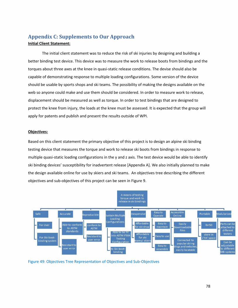
78
Appendix C: Supplements to Our Approach Initial Client Statement:
The initial client statement was to reduce the risk of ski injuries by designing and building a
better binding test device. This device was to measure the work to release boots from bindings and the
torques about three axes at the knee in quasi-static release conditions. The devise should also be
capable of demonstrating response to multiple loading configurations. Some version of the device
should be usable by sports shops and ski teams. The possibility of making the designs available on the
web so anyone could make and use them should be considered. In order to measure work to release,
displacement should be measured as well as torque. In order to test bindings that are designed to
protect the knee from injury, the loads at the knee must be assessed. It is expected that the group will
apply for patents and publish and present the results outside of WPI.
Objectives:
Based on this client statement the primary objective of this project is to design an alpine ski binding
testing device that measures the torque and work to release ski boots from bindings in response to
multiple quasi-static loading configurations in the y and z axis. The test device would be able to identify
ski binding devices’ susceptibility for inadvertent release [Appendix A]. We also initially planned to make
the design available online for use by skiers and ski teams. An objectives tree describing the different
objectives and sub-objectives of this project can be seen in Figure 9.
Figure 49: Objectives Tree Representation of Objectives and Sub-Objectives

79
The main objectives of this project, in order of importance, are that the device needs to be safe for the
user, safe for the ski boot binding system, accurate, reproducible, able to sustain multiple loading
configurations, inexpensive, easy to assemble, maintain, and use, accessible online, portable, and
modularized. Modularization means that our final design, as opposed to our testing prototype, will be
compatible with a wide range of different binding testers, and that it will be independent from specific
supplementary release equipment. This objective is ranked lowest on our list because it was determined
that creating a preliminary testing device that articulated well with a Vermont Release Calibrator foot
prosthetic, the most common commercial tester in the US, was the primary focus. These objectives and
their order of importance were discussed and agreed upon with our advisor, as demonstrated in our
pairwise comparison chart [Table 1].
Table 35: Pairwise Comparison Chart of Objectives

80
Appendix D: CAD Drawings of System

81

82
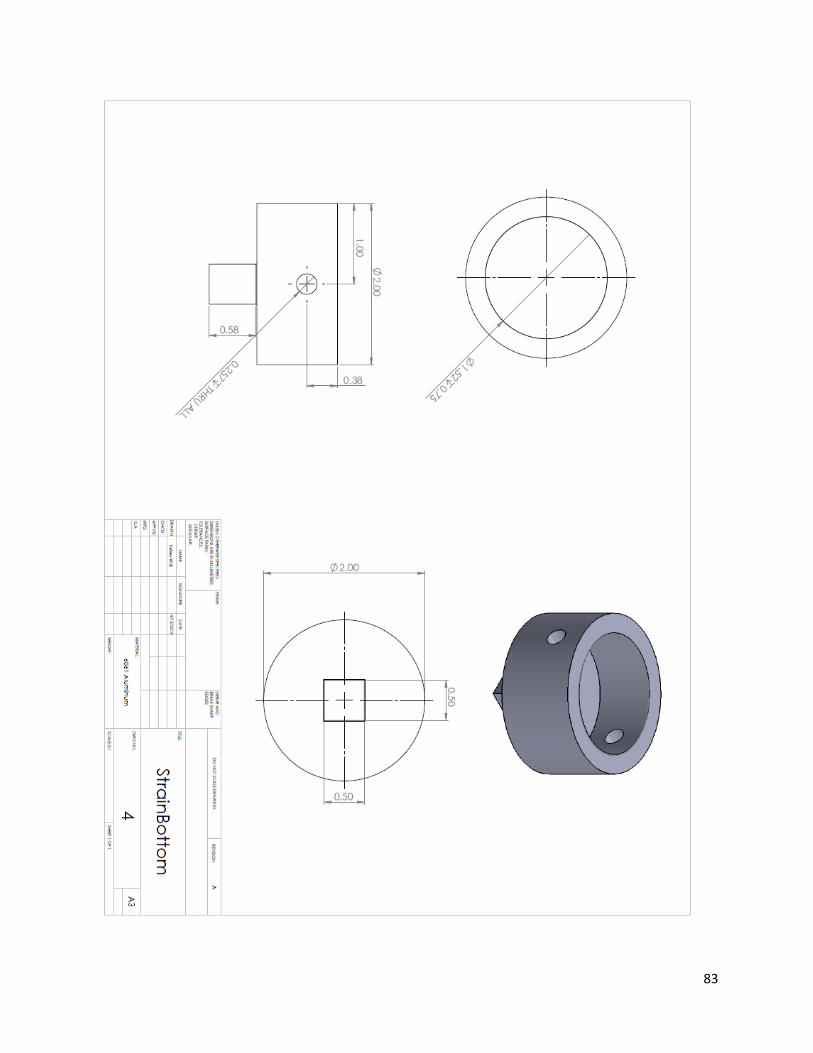
83

84

85

86
Appendix E: SignalExpress Instructions (NI, 2010)
DAQ Getting Started Guide This guide describes how to confirm your NI data acquisition (DAQ) device is operating properly. Install your application and driver software, then your device, using the instructions packaged with your device. Confirm Device Recognition Complete the following steps: 1. Double-click the Measurement & Automation icon on the desktop to open MAX. 2. Expand Devices and Interfaces to confirm your device is detected. If you are using a remote RT target, expand Remote Systems, find and expand your target, and then expand Devices and Interfaces. If your device is not listed, press <F5> to refresh MAX. If the device is still not recognized, refer to ni.com/support/daqmx.
Figure 50: MAX Configuration
For a Network DAQ device, do the following: • If the Network DAQ device is listed under Devices and Interfaces»Network Devices, right-click it and select Add Device. • If your Network DAQ device is not listed, right-click Network Devices, and select Find Network NI-DAQmx Devices. In the Add Device Manually field, type the Network DAQ device’s host name or IP address, click the + button, and click Add Selected Devices. Your device will be added under Devices and Interfaces»Network Devices (Figure 50). Note If your DHCP server is set up to automatically register host names, the device registers the default host name as cDAQ<model number>-<serial number>, WLS-<serial number>, or
Attach sensors and signal lines to the terminal block or accessory terminals for each installed device. Table 36 lists device terminal/pinout locations.

87
Table 36: Terminal/pin locations
Use NI-DAQmx with Your Application Software The DAQ Assistant is compatible with version 8.2 or later of LabVIEW, version 7.x or later of LabWindows™/CVI™ or Measurement Studio, or with version 3 or later of LabVIEW SignalExpress. LabVIEW SignalExpress LE, an easy-to-use configuration-based tool for data logging applications, is at Start»All Programs»National Instruments»LabVIEW SignalExpress. To get started with data acquisition in your application software, refer to the tutorials seen in Table 37: Table 37: Location for software tutorials
Examples NI-DAQmx includes example programs to help you get started developing an application. Modify example code and save it in an application, or use examples to develop a new application or add example code to an existing application. To locate LabVIEW, LabWindows/CVI, Measurement Studio, Visual Basic, and ANSI C examples, go to ni.com/info and enter the info code daqmxexp. For additional examples, refer to zone.ni.com. To run examples without hardware installed, use an NI-DAQmx simulated device. In MAX, select Help»Help Topics»NI-DAQmx»MAX Help for NI-DAQmx and search for simulated devices. Troubleshooting If you have problems installing your software, go to ni.com/support/daqmx. For hardware troubleshooting, go to ni.com/support and enter your device name, or go to ni.com/kb. If you need to return your National Instruments hardware for repair or device calibration, refer to ni.com/info and enter the info code rdsenn to start the Return Merchandise Authorization (RMA) process. Go to ni.com/info and enter rddq8x for a complete listing of the NI-DAQmx documents and their locations.

88
Appendix F: Clockwise SBB System Torque vs. Time Graph
Figure 51: A compilation of all torque vs time graphs generated during clockwise SBB system testing
0
20
40
60
80
0 2 4 6
Torq
ue
(Nm
)
Time (sec)
Clockwise Testing with SBB System Run 1
0
20
40
60
80
0 2 4 6
Torq
ue
(Nm
)
Time (sec)
Clockwise Testing With SBB System Run 2
0
20
40
60
80
0 2 4 6 8
Torq
ue
(Nm
)
Time (s)
Clockwise Testing with SBB Sytem Run 3
0
20
40
60
80
0 2 4 6
Torq
ue
(Nm
)
Time (sec)
Clockwise Testing With SBB System Run 4
0
20
40
60
80
0 2 4 6 8
Torq
ue
(Nm
)
Time (sec)
Clockwise Testing with SBB System Run 5
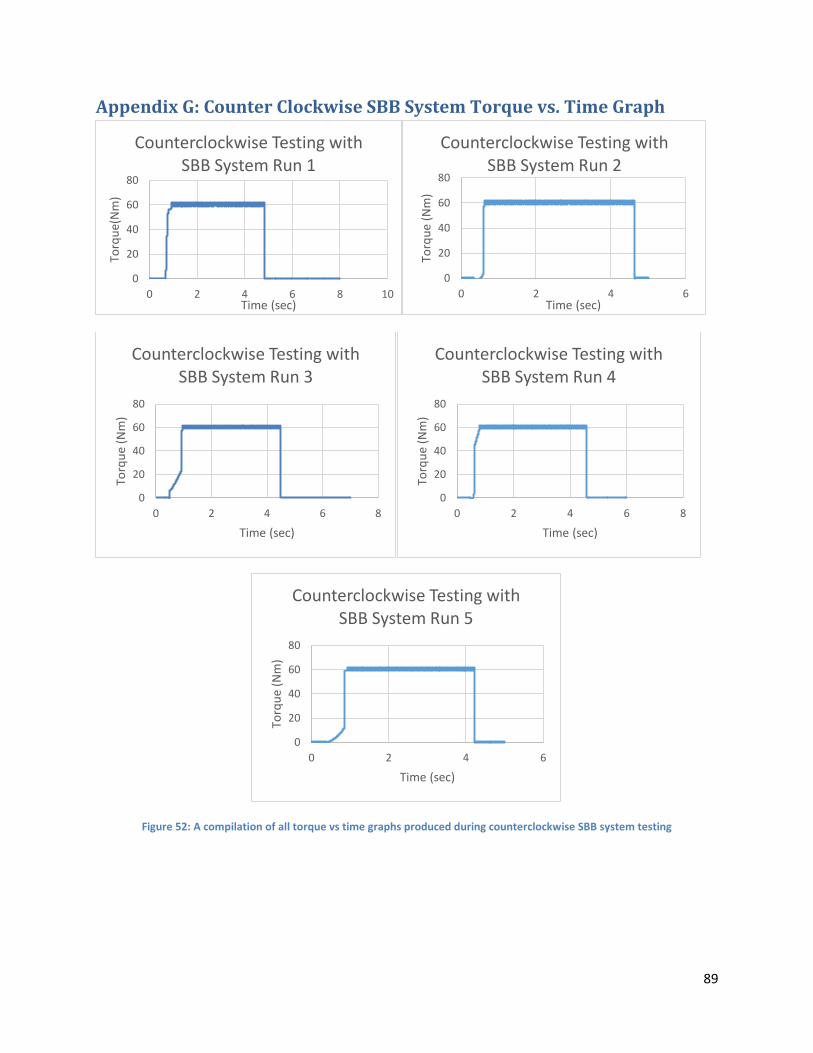
89
Appendix G: Counter Clockwise SBB System Torque vs. Time Graph
Figure 52: A compilation of all torque vs time graphs produced during counterclockwise SBB system testing
0
20
40
60
80
0 2 4 6 8 10
Torq
ue(
Nm
)
Time (sec)
Counterclockwise Testing with SBB System Run 1
0
20
40
60
80
0 2 4 6
Torq
ue
(Nm
)
Time (sec)
Counterclockwise Testing with SBB System Run 2
0
20
40
60
80
0 2 4 6 8
Torq
ue
(Nm
)
Time (sec)
Counterclockwise Testing with SBB System Run 3
0
20
40
60
80
0 2 4 6 8
Torq
ue
(Nm
)
Time (sec)
Counterclockwise Testing with SBB System Run 4
0
20
40
60
80
0 2 4 6
Torq
ue
(Nm
)
Time (sec)
Counterclockwise Testing with SBB System Run 5

90
Appendix H: Optical Mouse Data Analysis In order to successfully validate a device as a capable displacement sensor, several criteria must be met.
Established system constraints must be considered; both cost of the device and its precision capabilities.
The tolerance and precision of the device must satisfy ISO 9462 return-to-center test. This test requires
that the boot return to within 2mm of the binding’s center, requiring a precision 1/10th of that
measurement. A displacement sensor for this system must meet these previously established
constraints of the project; sensor uncertainty must be within ±0.2 mm and remain within the project
budget. Uncertainty was defined using the standards described in ASTM E2655, which defines
uncertainty as “an indication of the magnitude of error associated with a value that takes into account
both systematic errors and random errors associated with the measurement or test process” (ASTM
E2655, 2008). The equation for uncertainty from ASTM E2655 is as follows:
Where σ= the standard deviation, and n= the number of measurements
n= the number of measurements x=the sample = the sample mean A displacement sensor must also be capable of integration with the torque-to-release sensor. This
electronic integration should be a simple as possible, increasing chances of sustained accurate
measurements.
An optical mouse converts an electromagnetic signal, or light, to an electrical signal. This is
accomplished by reflecting LED light off a surface onto a CMOS (complementary metal-oxide
semiconductor) sensor. This sensor compares these reflected images thousands of times per second
with a Digital Signal Processor. Position is then determined relative to translation motion between
frames (Ng, 2003).
An electronic mouse provides several benefits as a potential displacement sensor. Optical mice offer
accurate sensing at nearly 2% of the cost of other conventional displacement sensors (Merrill, 2013).

91
Due to high production volumes, a “high-precision” mouse can be obtained for less than $20.
Additionally, a 2003 study by T.W. Ng of the National University of Singapore determined that an optical
mouse can be used as effective displacement sensor for small distances on an opaque surface.
Displacement of 1mm in both horizontal and vertical directions was performed; a mean square error of
0.018mm2 and a mean R2 value of 0.9914 was determined (Ng, 2003). These specifications were
satisfactory motives to perform further testing in regards to the boot-binding application.
H.1 Testing Setup and Procedure
H.1.1 Labview Program for Tracking Mouse Position
Electronic integration is a necessity for displacement measurements. A mouse’s movements across the
screen can easily be tracked using National Instrument’s Labview. A Virtual Instrument can be created
in order to track the x and y position of the cursor in relation to time. Using an ‘Initialize Mouse’
command to Generate Data, the x and y coordinates can be bundled together with a time stamp.
Mouse position is tracked relative to an origin in the top left corner of the screen (0,0). As the mouse
moves, the cursor on the screen displaces a certain number of dots, or pixels. This change in position
can be calibrated by measuring a known distance, a function relating actual displacement to pixel
displacement can be calculated. Validation of the precision, repeatability and linearity of the output
data is paramount for an accurate function.
By setting additional parameters, 100 data points are measured over a 5 second collection period. The
start of data collection is prompted by keystroke. This removes user interaction with the mouse,
increasing simplicity and mitigating potential sources of error. Using Labview ‘Write’ functions, all data
is labeled and exported to Excel. Figure 53 below shows the Virtual Instrument for collecting mouse
position.

92
Figure 53: Labview program for documenting mouse position
H.1.2 Physical Testing Setup
The position data that was recorded using Labview was obtained while the team moved an optical
mouse by a known increment. To do so required a test setup with two hard stops to ensure repeatable
displacement. These stops were positioned to ensure that the mouse would travel 30mm for initial tests
with a standard mouse. However, this increment was changed to 10mm, while using the 2000 DPI
gaming mouse, as larger displacements would cause the cursor of the mouse to reach the edge of the
computer screen. This was done so that the position, in units, of the mouse recorded through the
Labview Program could be compared to the known distance traveled by the mouse. Measuring the
length of the mouse and the distance between the hard stops will yield the amount of travel by the
mouse. As seen in Figure 54 below, this test setup was performed to verify y-axis displacement.
Figure 54: Physical test setup for mouse position data acquisition

93
A mouse is a sensitive sensor. With every small movement of the mouse, the cursor is displaced on the
screen by a certain amount of pixels, depending on the sensitivity settings of the mouse. The sensitivity
of a mouse is a user defined setting; defining the ratio of pixels displaced per centimeter displaced. This
setting can be adjusted from the ‘Control Panel’ window (Figure 55).This setting has a large effect on
precise displacement measurements, as a higher setting corresponds to a higher ratio of pixels to
centimeters displaced. Several experiments were conducted in order to establish the most effective
displacement sensor settings with this application.
Figure 55: Changing the pointer speed, or sensitivity, of an optical mouse
H.1.3 Data and Analysis
Linear displacement can be found using the function:
Where x is the change in x position and y is the change in y position. Using Labview, the position of
the mouse was tracked along the rigid path. In order to simplify the validation, only motion along the y
axis was tracked. It was found easiest to apply the displacement function within the raw Excel data;
however built-in functions within the VI could be applied.
Using the initial starting point as an offset, and .
Displacement was then calculated accordingly, as seen in Table 38.

94
Table 38: Mouse position and linear displacement calculations
Preliminary trials analyzed the mouse at speed, or sensitivity, settings 1, 5, and 10. Hard stops were
placed so that the mouse would only displace 30 millimeters. 100 data points were recorded per run
and linear displacement was recorded. The mean amount displaced, in unspecified units, was taken to
correlate to 30mm of displacement. Seven identical tests revealed the range, standard deviation and
uncertainty of mouse displacement measured through the Labview program. Tables 39, 40, and 41
correspond to the measurements obtained with a standard optical mouse at pointer speeds 1, 5, and 10,
respectively.
Table 39: Displacement measurements obtained by a standard mouse at pointer speed 1
Test #
Linear Displacement (units)
Linear Displacement (mm)
Average Linear Displacement (mm) Displacement (mm)
1 405.36 42.42 30.00 Average 30.00
2 330.12 34.55 S.D. 6.55
3 265.70 27.80 Uncertainty 2.67
4 253.34 26.51
5 241.30 25.25
6 224.29 23.47

95
Table 40: Displacement measurements obtained by a standard mouse at pointer speed 5
Test #
Linear Displacement (units)
Linear Displacement (mm)
Average Linear Displacement (mm) Displacement (mm)
1 597.55 27.29 30.00 Average 30.00
2 718.10 32.79 S.D. 1.85
3 692.06 31.60 Uncertainty 0.76
4 664.08 30.33
5 621.43 28.38
6 648.44 29.61
Table 41: Displacement measurements obtained by a standard mouse at pointer speed 10
Test #
Linear Displacement (units)
Linear Displacement (mm) Average Linear
Displacement (mm) Displacement (mm)
1 852.00 32.50 30.00 Average 30.00
2 838.01 31.96 S.D. 1.67
3 747.01 28.49 Uncertainty 0.68
4 782.03 29.83
5 738.02 28.15
6 762.00 29.07
Overall, the minimum uncertainty was found with the mouse at the highest and most sensitive speed;
setting 10. With a standard deviation of 1.67, this was our best result. The range of calculated
displacement was 28.15mm to 32.50mm. With an uncertainty of 0.68, the mouse does not preliminary
meet our constraints.
A mouse setting of 10 also creates additional sources of error. The high speed of the cursor limits the
amount of measureable displacement due to screen size. With the high speed setting, more pixels are
displaced per millimeter moved and the cursor will hit the edge of the screen with less movement.
With that in mind, an ideal setting of 7 was used for final testing. This would provide a maximum
sensitivity and mitigate the likelihood of the cursor hitting the side of the screen. A precise, high dot-
per-inch wireless mouse was also purchased. With 2000 dpi, this mouse is designed for performance.
Table 42 and figure 56 correspond to the measurements obtained with the 2000 dpi mouse at a pointer
speed setting of 7.

96
Table 42: Displacement measurement from a 2000 DPI mouse at pointer speed 7
Figure 56: Mean and standard deviation of mouse displacement measurements from a 2000 DPI mouse at pointer speed 7
This trial was our most successful, but still not within constraints. With a standard deviation of 0.75,
uncertainty for these trials is 0.28. These results would be considered promising for a mouse as a
displacement sensor, but there were many additional negative characteristics of the electronic mouse in
this application. Additionally, using a 2000 DPI mouse at pointer speed 7, restricts the user to
displacements within 10mm, which is unsuitable for this application. This means the low uncertainty
measured at this setting was meaningless, as it could not be used with a ski boot binding test setup.
H.1.4 Findings
Despite the findings of other scholarly works, testing was performed to fully validate linearity,
repeatability and uncertainty within the scope of our design. Despite exhaustive experimentation
(Appendix H), the level of uncertainty of an electronic mouse was not within our constraint of 0.2 mm.
Despite a rated resolution of 2000 dpi, an optical mouse is not a viable sensor in this application.
Several sources of error were analyzed and documented.
0.00
2.00
4.00
6.00
8.00
10.00
12.00
Trial
Setting 10: Linear Displacement (mm)
Test # Displacement (units) Displacement (mm) Average Linear
Displacement (mm) Total Displacement (mm)
1 680.00 9.32 10.00 Average 10.00
2 795.00 10.90 S.D. 0.75
3 720.00 9.87 Uncertainty 0.28
4 728.00 9.98
5 745.00 10.22
6 724.00 9.93
7 713.00 9.78

97
Firstly, an optical mouse’s accuracy is strictly dependent on a precise z-axis distance. With any
separation from the imaging surface, the mouse becomes inoperable. In binding testing procedures the
boot may twist and roll along the x-axis creating z-axis separation. This is difficult to mitigate in a
binding test. A third source of error with a mouse is top speed. Binding testing is to be performed with
applied torque for a maximum of 5 seconds (ASTM, 2009). This quick release may be difficult to capture
with an electronic mouse, a 1000 dpi gaming mouse has a top speed around 0.5 m/s (Windows, 2002).
This is not adequate for this application.
Additional error can be incurred due to smoothing or anti-aliasing functions built in to the mouse
hardware. Designed to smooth the translation of the cursor on the screen, these minor adjustments can
affect trajectory across the screen as well as cause significant lag. These properties will dramatically
decrease the accuracy of a computer mouse. Lastly, screen size will limit the amount of recordable
displacement distance. If the cursor runs into the edge of the screen during testing, data is halted at
that point. This limitation requires additional preliminary setup, and may go unnoticed.

98
Appendix I: Polaris Measurement Analysis
I.1 Test Setup Our displacement measurements were made by applying removable fiduciaries, also known as passive
markers, onto the tested ski boot in order for the Polaris Spectra to optically track the three-dimensional
motion of the boot, while other passive markers were used to provide a reference frame for the
displacement (Figure 57). This setup was placed approximately 5 feet from the NDI Polaris sensor. The
passer markers on the toe of the boot can be seen extending above, while the reference markers are on
the tabletop in front.
Figure 57: Ski boot with attached passive marker and passive marker reference marker on testing bench
The position of the boot in relation to the reference marker was determined by the Polaris’ optical
measurement system and Application Program Interface (API), which allowed for tracking of specific
passive markers and output data to Excel. During Polaris testing, the position of the tracking markers
was measured and recorded via calipers, and then compared to the positions documented by the Polaris
to validate the precision of the measurements. The passive marker affixed to the ski boot, was aligned
with the mid-sole line of the boot, which was moved to a rigidly defined point. Error analysis of the

99
reported data was conducted in order to determine the sensors viability in a torque-displacement
testing system.
I.2 Data and Analysis The passive markers are tracked in 3D space relative to the reference passive marker, in centimeters, as
x, y and z coordinates within the measurement volume. The output relative position is provided on a
frame basis, but does not include a timestamp to identify the time at which these positions were
documented. The output data is sent to a CSV file format in Excel, and includes the error associated with
each position documented in the frame (Table 43).
Table 43: Polaris position tracking of a ski boot
A series of four identical tests were performed to assess error in the system. Error analysis was
performed by averaging the 500 error values provided by the Polaris (Table 44).

100
Table 44: Average Polaris Error (cm)
Average System Error (cm)
Test #1 Test #2 Test#3 Test#4 System Error
0.14 0.19 0.20 0.12 0.16
A total average error was calculated to be 0.16cm, or 1.6mm. This level error, and lack of certainty, is
far greater than is tolerable for this application.
Unfortunately, these results were expected with the NDI Polaris. A nominal error of the system is
claimed to be as low as 0.3mm, but results show that the value was much larger. Similar to other similar
technology, these sensors are more imprecise at distances and do not respond well to quick, sudden
motions. This system is not designed to measure small displacements, and therefore this technology is
ineffectual.

101
Appendix J: Prototype and Consumer Costs
Prototype Costs Stock Materials (Total): $54.71 6061 Aluminum Rod, 2” Diameter, 1’ Length $23.99
6061 Aluminum Tube, 1-1/2" OD, 1" ID, .250" Wall Thickness, 1' Length $18.07
6061 Aluminum Tube, 1-1/2" OD, 1.402" ID, .049" Wall Thickness, 1' Length $12.65
304 Stainless Steel Rectangular Tube Stock Provided (Epitaux Lever)
Circuit Components (Total): $6.78 Resistors Provided
Wiring Provided
2 INA217AIP Amplifiers $6.78
National Instruments USB-6008 DAQ: Provided
Vermont Release Calibrator Prosthetic Foot: Provided Labview SignalExpress Software and NI-MAX Drivers: Provided
Total Prototype Costs $61.49
Consumer Costs CNC Manufacturing (2 Hours): $50 McMaster-Carr Stock Materials (Total): $91.78 6061 Aluminum Rod, 2” Diameter, ½’ Length $16.36 6061 Aluminum Tube, 1-1/2" OD, 1" ID, .250" Wall Thickness, 1'
Length $10.84
6061 Aluminum Tube, 1-1/2" OD, 1" ID,
0.049" Wall Thickness, 1/2' Length $7.59
304 Stainless Steel Rectangular Tube Stock $56.99 DigiKey Circuit Components (Total): $7.78 Resistors: $0.20 Wiring: $0.80 2 INA217AIP Amplifiers: $6.78 National Instruments USB-6008 DAQ: $189 Vermont Release Calibrator Prosthetic Foot: $200 Labview SignalExpress Software and NI-MAX Drivers: Free Total Consumer Cost (with Prosthetic Foot) $538.56
Total Discluding Including Prosthetic Foot $338.56

102
References AMES. (2013). ANSI Standard Limits and Fits Calculator. Advanced Mechanical Engineering Solutions.
Retrieved December 12, 2013, From: http://www.amesweb.info/FitTolerance/FitToleranceImperial.aspx
ASM. (2013). Aluminum 6061-T6; 6061-T651. Aerospace Specification Metals Inc. Retrieved December
18, 2013, From: http://asm.matweb.com
ASTM. (2005). Standard Practice for Selection of Release Torque Values for Alpine Ski Bindings. ASTM
Standards. Pennsylvania, United States of America: American Society for Testing and Materials.
ASTM. (2008). Standard Specification for Ski Binding Test Devices. ASTM Standards. Pennsylvania,
United States of America: American Society for Testing and Materials.
ASTM E2655. (2008).Standard Guide for Reporting Uncertainty of Test Results and Use of the Term
Measurement Uncertainty in ASTM Test Methods. ASTM Standards. Pennsylvania, United States of
America: American Society for Testing and Materials.
ASTM. (2009). Standards for Functional Inspections and Adjustments of Alpine Ski/Binding/Boot
Systems. ASTM Standards. Pennsylvania, United States of America: American Society for Testing and
Materials.
ASTM. (2013). Standard Method for Verification of Ski Binding Test Devices. ASTM Standards.
Pennsylvania, United States of America: American Society for Testing and Materials.
BEI Sensors. (2014). Optical Rotary Encoders-Incremental versus Absolute and Shafted versus Hollow
Shaft Encoder Products. From: http://www.beisensors.com/technical-support-bei-rotary-encoder-vs-
optical-encoder.html
Beynnon, B. D., Ettlinger, C. F., Johnson, R. J., Natri, A., & Shealy, J. E. (1997). Alpine ski bindings and
injuries. Sports medicine, 28(1), 35-48.
Brown, C. A. (2006). Axiomatic Design and the Evolution of Conventional Alpine Ski Bindings. Retrieved
June 1, 2013, from Axiomatic Design:
http://www.axiomaticdesign.org/docs/AxiomaticDesignandSkiBindings.pdf
Brown, C. A., & Ettlinger, C. F. (1985). A method for improvement of retention characteristics in alpine
ski bindings. In Skiing Trauma and Safety: Fifth International Symposium (ASTM STP 860). Philadelphia,
PA: ASTM International (pp. 224-237).
CDC. (2010). Anthropometric Reference Data for Children and Adults: United States 2007-2010. Centerd
for Disease Control and Prevention. From: http://www.cdc.gov/nchs/data/series/sr_11/sr11_252.pdf
Dodge, D., Ettlinger, C. F., Johnson, R. J., Sargent, M., and Shealy, J. E. (2010) Retention requirements for
alpine ski bindings Journal of ASTM International, Vol. 7, No. 6.

103
Epitaux, Jacques. (1989). U.S. Patent No. 4,860,595. Washington, DC: U.S. Patent and Trademark Office
Ettlinger, Carl F. (1974). U.S. Patent No. 3,805,603. Washington, DC: U.S. Patent and Trademark Office
Ettlinger, C. F., Johnson, R. J., & Shealy, J. E. (2005). Using signal detection theory as a model to evaluate
release/retention criteria in alpine skiing. Journal of ASTM International(JAI), 2(7).
Ettlinger, C. F., Shealy, J. E., & Johnson, R. J. (2009). Myths Concerning Alpine Skiing Injuries Sports
Health: A Multidisciplinary Approach, 1(6), 486-492.
Ettlinger, C. (2010). FAQ #5 for Skiers/ Riders. Retrieved May 28th, 2013, from Vermont
Ski Safety: http://www.vermontskisafety.com/
Hawks, T. (2012, October 1). NSAA Fact Sheet. Retrieved May 30th, 2013, from National Ski Areas
Association Website: www.nsaa.org
Hoffmann, K. (1986). Applying the Wheatstone Bridge Circuit. HBM S1569-1.1 en, HBM, Darmstadt,
Germany, http://www. hbm. com/fileadmin/mediapool/hbmdoc/technical/s1569. pdf.
ISO. (2009). Alpine ski bindings- Requirements and test methods. International Standards and British
Standards. London, England: British Standards Institution.
Jones, F. D., Oberg, E., & Horton, H. L. (2004). Machinery's handbook. Industrial Press, Incorporated.
Lagran, M. (2012). Head Injuries on the Slopes. Retrieved: May 31st, from: Ski Injury
http://www.ski.injury.com
LeapMotion. (2014). Explore the World in a Whole New Way. Retrieved: February 12th, 2014
From: https://www.leapmotion.com/product
Lipe, Gordan C. & Hinds, Charles W. (1966). U.S. Patent No. 3,289,472. Washington, DC: U.S. Patent and
Trademark Office.
Merrill, Bradley. (2013). Torque-Displacement Binding Tester (Undergraduate Interactive Qualifying
Project, E-project-031213-113928). Retrieved from Worcester Polytechnic Institute Electronic Projects
Collection: http://www.wpi.edu/Pubs/E-project/Available/E-project-031213-113928/
NDI. (2014). Polaris Optical Tracking System. NDI Medical. Retrieved From:
http://www.ndigital.com/medical/products/polaris-family/
New York Times. (2008, March 4). Alpine Skiing Men’s World Cup. Retrieved July, 3 2013, from The New
York Times: http://www.nytimes.com/2008/03/04/sports/04ihtalpine4.10693330.html
Ng, T. W. (2003). The optical mouse as a two-dimensional displacement sensor. Sensors and Actuators A:
Physical, 107(1), 21-25.

104
NI. (2010). DAQ Getting Started Guide. National Instruments. From:
http://www.ni.com/pdf/manuals/373737d.pdf
National Instruments. (2014). NI SignalExpress. From: http://www.ni.com/labview/signalexpress/
Özkaya, N., Nordin, M., Goldsheyder, D., & Leger, D. (2012). Fundamentals of biomechanics: equilibrium,
motion, and deformation. Springer.
Paletta, G. A., & Warren, R. F. (1994). Knee injuries and alpine skiing. Sports Medicine, 17(6), 411-423.
Shealy, J. E., Ettlinger, C. F., & Johnson, R. J. (1999). Signal Detection Theory: A Model for Evaluating
Relense/Retention Criteria in Alpine Ski-Binding-Boot Systems. ASTM SPECIAL TECHNICAL
PUBLICATION, 1345, 120-131.
Ski Gear TV (2012, December 8). Ski Prophet Presents Core Shot: Ski Binding Test [Video file]. Retrieved
from http://www.youtube.com/watch?v=ORvpLjlx8Uk
SIA. (March, 2013). 2013 SIA Snow Sports Fact Sheet. Retrieved September 12th, from: Snow Sports
Industries America website: www.snowsports.org
Suh, N. P. (1990). The principles of design. New York: Oxford University Press.
Taylor, B. N. (2009). Guidelines for Evaluating and Expressing the Uncertainty of NIST Measurement
Results (rev. DIANE Publishing.
Texas Instruments. (2005). Low-Noise, Low-Distortion Instrumentation Amplifier Replacement for
SSM2017. Retrieved from: http://www.ti.com/lit/ds/symlink/ina217.pdf
Vishay Precision Group. (2011, December 19). Surface Preparation for Strain Gage Bonding. Retrieved
December 2013, from VishayPG.com.
Vermont Ski Safety (2010). Vermont release calibrator operation and maintenance manual.
Retrieved July 9, 2013, from http://www.vermontskisafety.com/files/CALIBRATER-MANUAL.pdf
Wiles, A. D., Thompson, D. G., & Frantz, D. D. (2004, May). Accuracy assessment and interpretation for
optical tracking systems. In Medical Imaging 2004 (pp. 421-432). International Society for Optics and
Photonics.
Windows. (2002). Pointer ballistics for Windows XP. Windows Hardware Developer Center Archive.
Microsoft
Wintersteiger (2011). Speedtronic Pro. Retrieved June 30, 2013, from
http://www.wintersteiger.com/us/Sports/Machines/New-Machines/Binding-adjustment/84-
Speedtronic-Pro/
Young, L. R. (1989). Elevated racer binding settings and inadvertent releases. In Skiing trauma and
safety. Seventh International Symposium, ASTM STP (Vol. 1022, pp. 222-7).