an agglomeration multigrid method for unstructured grids · an agglomeration multigrid method for...

Contemporary MathematicsVolume 218, 1998

An Agglomeration Multigrid Method for Unstructured Grids

Tony F. Chan, Jinchao Xu, and Ludmil Zikatanov

1. Introduction

A new agglomeration multigrid method is proposed in this paper for generalunstructured grids. By a proper local agglomeration of finite elements, a nestedsequence of finite dimensional subspaces are obtained by taking appropriate linearcombinations of the basis functions from previous level of space. Our algorithmseems to be able to solve, for example, the Poisson equation discretized on anyshape-regular finite element grids with nearly optimal complexity.

In this paper, we discuss a multilevel method applied to problems on generalunstructured grids. We will describe an approach for designing a multilevel methodfor the solution of large systems of linear algebraic equations, arising from finiteelement discretizations on unstructured grids. Our interest will be focused on theperformance of an agglomeration multigrid method for unstructured grids.

One approach of constructing coarse spaces is based on generating node-nestedcoarse grids, which are created by selecting subsets of a vertex set, retriangulatingthe subset, and using piecewise linear interpolation between the grids (see [8, 5]).This still provides an automatic way of generating coarse grids and faster implemen-tations of the interpolation in O(n) time. The drawback is that in three dimensions,retetrahedralization can be problematic.

Another effective coarsening strategy has been proposed by Bank and Xu [1].It uses the geometrical coordinates of the fine grid and the derefinement algorithmis based on the specified patterns of fine grid elements. The interpolation betweengrids is done by interpolating each fine grid node using only 2 coarse grid nodes.As a consequence of that the fill-in in the coarse grid matrices is reasonably small.The hierarchy of spaces is defined by interpolating the basis.

Recently a new approach, known as auxiliary space method, was proposed byXu [16]. In this method only one non-nested (auxiliary) grid is created and then allconsecutive grids are nested. This can be done by using as auxiliary grid a uniform

1991 Mathematics Subject Classification. Primary 65N55; Secondary 35J05.The first author was supported in part by NSF ASC-9720257.The second author was supported in part by NSF DMS94-03915-1 and NSF DMS-9706949

through Penn State, by NSF ASC-92-01266 through UCLA and NSF ASC-9720257.The third author was supported in part by NSF DMS-9706949 through Penn State, NSF ASC-

9720257 and also by Center for Computational Mathematics and Applications of PennsylvaniaState University.

c©1998 American Mathematical Society

67

Contemporary Mathematics

Volume 218, 1998

B 0-8218-0988-1-03002-8

68 TONY F. CHAN ET AL.

one and interpolating the values from the original grid there. For a uniform gridthen, there is a natural hierarchy of coarse grids and spaces. Such a procedure leadsto optimal multigrid methods in some applications.

One promising new coarsening techniques is based on the agglomeration tech-nique (see Koobus, Lallemand and Dervieux [11]). Instead of constructing aproper coarse grid, neighboring fine grid elements are agglomerated together toform macroelements. Since these agglomerated regions are not standard finite ele-ments, appropriate basis functions and interpolation operators must be constructedon them. An algebraic construction of agglomerated coarse grid spaces has beeninvestigated by Vanek, Mandel, and Brezina [6] and Vanek, Krızkova [7]. Theirapproach uses a simple initial interpolation matrix, which might not be stable, andthen this matrix is smoothed and stabilized by some basic relaxation schemes, e.g.Jacobi method.

The pure algebraic definition of the coarse spaces has the advantage that thereis no need to use any geometrical information of the grid or of the shape of the gridand the kind of finite elements used. We refer to a paper by Ruge and Stuben [13]on algebraic multigrid. Recent developments in this direction have been made byBraess [2] and Reusken [12]. The main issue in using pure “black-box” algebraicderefinement is that the coarse grid operators usually become denser and it is notclear how to control their sparsity except in some special cases.

Another approach in the definition of coarse spaces, known as composite finiteelement method was recently investigated by Hackbusch and Sauter in [10]. Thismethod gives coarse space constructions which result in only few degrees of freedomon the coarse grid, and yet can be applied to problems with complicated geometries.

In this paper, we will consider a new and rather simple technique for definingnested coarse spaces and the corresponding interpolation operators. Our earlierexperience shows that the definition of the sparsity pattern of the transfer opera-tors and the definition of these operators themselves is the most crucial point indesigning multigrid algorithms for elliptic problems. In the present paper we pro-pose a technique based on the graph-theoretical approach. Our goal is to constructa “coarse grid” using only the combinatorial (not the geometrical properties) ofthe graph of the underlying fine grid. This coarse grid is formed by groups of el-ements called agglomerated macroelements. Using this approach a macroelementgrid can be constructed for any unstructured finite element triangulation. We canimplement our algorithm with or without any use of the nodal coordinates. Basedon this macroelement partition, we propose an interpolation technique which usesonly arithmetic average based on clearly determined coarse grid nodes. This leadsto savings in storage and CPU time, when such scheme is implemented. In fact,to store the interpolation matrix we only need to store integers. Although rathersimple, such type of interpolation leads to a multigrid algorithm with nearly opti-mal performance. Moreover the algorithm naturally recovers the structure of thenatural coarse grids if the fine grid is obtained by structured refinement. Althoughwe present only 2D algorithms we believe that it can be extended for 3D problemsas well.

The rest of the paper is organized as follows. In section 2 we state the differen-tial problem and briefly comment on the finite element discretization. In section 3we give the definition of the standard V -cycle preconditioner. In section 4 we de-scribe in detail the two level coarsening algorithm. In section 4.3 the interpolationbetween grids is defined. The multilevel implementation of the algorithm is given

AN AGGLOMERATION MULTIGRID METHOD FOR UNSTRUCTURED GRIDS 69

in Section 4.4. The stability and approximation properties are investigated in Sec-tion 5 under rather mild assumptions on the geometry of the coarse grids. InSection 6 results of several numerical experiments are presented.

2. A model problem and discretization

Let Ω ⊂ IR2 be a polygonal domain with boundary Γ = ΓD ∪ ΓN , where ΓD isa closed subset of Γ with positive measure. We consider the following variationalformulation of elliptic PDE: Find U ∈ H1

D(Ω) such that

a(U, v) = F (v) for all v ∈ H1D(Ω),(1)

where

a(U, v) =∫

Ωα(x)∇U · ∇vdx, F (v) =

∫ΩF (x)vdx.(2)

Here H1D(Ω) as usual denotes the Sobolev space which contains functions which

vanish on ΓD with square integrable first derivatives. It is well-known that (1)is uniquely solvable if α(x) is a strictly positive scalar function and F is squareintegrable.

We consider a finite element space of continuous piecewise linear functionsMh ⊂ H1

D(Ω) defined on a triangulation Th of Ω. Then the corresponding finiteelement discretization of (2) is: Find uh ∈Mh such that

a(uh, vh) = F (vh) for all vh ∈Mh.(3)

The discretization results in a linear system of equations:

Au = f,(4)

where A is a symmetric and positive definite matrix, f is the right hand side andthe nodal values of the discrete solution uh will be obtained in the vector u aftersolving the system (4).

3. Multigrid method

In this section, we introduce the notation related to the multigrid method, andwe define the (1-1) V -cycle preconditioner.

Let us consider the following simple iteration scheme:

u`+1 = u` +BJ(f −Au`) ` = 1, 2, . . . ,(5)

where BJ is the V -cycle preconditioner BJ to be defined. We assume that wehave given a nested sequence of subspaces M0 ⊂ . . . ⊂ MJ−1 ⊂ MJ ≡ Mh, withdim(Mk) = nk. We assume that the matrices Ak, k = 0, . . . J , are stiffness matricesassociated with Mk. We also assume that the interpolation operators Ikk−1 and thesmoothing operators Sk are given.

In our case BJ will correspond to (1 − 1) V -cycle preconditioner. For giveng ∈Mk we define Bkg as follows:

Algorithm 1. [(1-1) V -cycle ]


0. If k = 0 then B0g = A−10 g

1. Pre-smoothing: x1 = STk g2. Coarse grid correction:

1. q0 = (Ikk−1)T (g −Akx1);2. q1 = Bk−1q

0;3. x2 = x1 + Ikk−1q

1;3. Post-smoothing: Bkg = x2 + Sk(g −Akx2).

The practical definition of such a preconditioner in the case of unstructuredgrids will be our main goal in the next sections. We will define proper interpolation(prolongation) operators Ikk−1, for k = 1, . . . , J and the subspace Mk−1 by interpo-lating the nodal basis in Mk. In order to have convergence of the iteration (5) inde-pendent of the mesh parameters, the subspaces have to satisfy certain stability andapproximation properties, namely, that there exists a operator Πk : H1(Ω) → Mk

such that:

‖Πkv‖1,Ω ≤ C‖v‖1,Ω,(6)

‖v −Πkv‖0,Ω ≤ Ch|v|1,Ω, ∀v ∈ H1(Ω).(7)

We will comment on these properties of the agglomerated spaces in Section 5. Oncethe subspaces are defined, the V -cycle algorithm can be implemented in a straight-forward fashion using as coarse grid matrices, given by Ak−1 = (Ikk−1)TAkIkk−1.

General discussions concerning the convergence of this type of method andits implementation can be found in the standard references, e.g. Bramble [3],Hackbusch [9], Xu [15].

4. Agglomerated macroelements

The main approach we will take in the construction of Ikk−1 will be first to definea coarse grid formed by macroelements (groups of triangles) and then interpolatelocally within each macroelement. In this section, we will present an algorithm forthe definition of the coarse grid consisting of macroelements. We first identify theset of coarse grid nodes. The interpolation from coarse grid to the fine grid will usethe values at these nodes. As a next step, for a given node on the fine grid we haveto define its ancestors on the coarse grid (i.e. the coarse grid nodes which will beused in the interpolation). These ancestors are determined by partitioning the finegrid into agglomerated macroelements (such macroelements can be seen on Fig. 1)which in some sense are analogue of the finite elements, because they have verticeswhich are precisely the coarse grid nodes, and their edges are formed by edges ofthe underlying fine grid.

4.1. Some basic graph theory. In this subsection we introduce some basicnotation and definitions. Given a finite element triangulation Th of Ω, we considerthe corresponding graph, denoted by G = (V,E), where V is the set of vertices (gridnodes) and E is the set of edges (boundaries of the triangles). In this definition, theconcept of vertex and edge happen to be the same for the underlying triangulationand for the graph corresponding to the stiffness matrix. Associated with the graphG, we will form our coarse grid on the so called maximal independent set (MIS, forshort) which is a set of vertices having the following two properties: any two verticesin this set are independent in the sense that they are not connected by an edge,and the set is maximal in the sense that an addition of any vertex to the set willinvalidate the aforementioned independent property. The graph distance between


Figure 1. An example of macroelements

Figure 2. A triangulation and its dual mesh.

two vertices v, w ∈ V is defined to be the length of the shortest path between thesetwo vertices. A matching in G is any collection of edges such that no two edges inthis collection share a vertex.

The construction of the macroelements will be based on the dual mesh (graph)of G defined as follows. Given a triangulation Th and associated graph G, the dualgraph G′ = (V ′, E′) of G is:

• Each element T ∈ Th is a vertex in G′.• Two vertices in G′ are connected by an edge if and only if they share an

edge in G, i.e. (T1, T2) ∈ E′ if and only if T1 ∩ T2 ∈ E (see Fig. 2).

4.2. Two level coarsening algorithm. In this section we describe in detailthe heuristic algorithm for forming a coarse grid macroelements from a given finiteelement triangulation.

As a first step we define the set of coarse nodes to be a MIS in G. An MIS isobtained by a simple “greedy” (locally optimal) algorithm given as follows.


Figure 3. Connected components in G∗.

Algorithm 2 (MIS).1. Pick an initial set of vertices V0 (for example all boundary vertices).2. Repeat:

(a) Apply a “greedy” algorithm to find MIS in V0.(b) Mark all nodes at distance 1 from V0 (here distance is the graph

distance).(c) Take as V0 all vertices which are at distance 2 from V0 and have not

been explored (marked).3. until V0 = ∅.4. Complete MIS by applying one step of “greedy” algorithm on V .

To define the macroelements, we use the fact that separating two triangles onthe fine grid and putting them in different groups is equivalent to removing an edgein the dual graph G′.

We now describe how to form the initial partition of G into groups of elements.For any coarse grid node k (i.e. k ∈ MIS) we pick the edges in G having this

node as an end. To this set of edges Ek ⊂ E corresponds a set E′k ⊂ E′, namely E′kcontains exactly all edges between all T ∈ Th which have this particular coarse nodeas a vertex. As a first step we remove E′k from E′. Applying this procedure for allcoarse grid nodes results in a subgraph of G′, G∗ = (V ∗, E∗) where V ∗ = V ′ andE∗ = E′\ ∪k E′k. The connected components in G∗ will form the initial partitionof Ω into groups of elements (see Fig. 3).

We note that there might be some isolated vertices in G∗ and also some of theconnected components might be considerably large. We first deal with the largegroups (such a group can be seen on Fig. 3 in the right bottom corner of the domain)and we break them into smaller pieces. We consider a group of elements M ⊂ Ththat corresponds to one connected component in G∗ and denote the set of edges inM by EM . We intend to break this group in pieces if there is an “interior” edgee ∈ EM such that e∩ ∂M = ∅. This breakup is done as follows (our considerationshere are restricted only on M ⊂ Th):


• From the subgraph formed by all edges e ⊂ EM such that e ∩ ∂M = ∅, weform a matching. On the model grid (see Fig. 3) there is only one such edgein the whole domain.• Remove the edges in the dual corresponding to the edges in the matching.

In Fig. 3 this edge in the dual is drawn with thick line (near the right bottomcorner of the domain). The pieces obtained by removing this edge are clearlyseen on Fig. 1).

The situation with the isolated vertices in G∗ is simpler. We propose twodifferent ways of dealing with them as follows:

1. Since each isolated triangle (vertex in G∗) has as one vertex being a coarsegrid point, the edge opposite to this vertex does not have a coarse gridnode as an end, because our set of coarse grid nodes is a MIS. We grouptogether two neighbors sharing this edge to form a macroelement. If suchedge happens to be a boundary edge, we leave a single triangle to be amacroelement.

2. We group together all isolated neighbors. If such a group does not havemore than 4 coarse grid vertices then we consider it as a new agglomeratedmacroelement. If it has more than 4 coarse grid vertices we proceed as in theprevious step coupling triangles in this group two by two. In partitioningour model grid we have used precisely this way of grouping isolated triangles(see Fig 3, Fig. 1).

It is obvious that all triangles from the triangulation are either in a connectedcomponent in G∗ or are isolated vertices in G∗. Thus we have explored all thetriangles and every T ∈ Th is in some macroelement (see Fig. 1).

To summarize we give the following short description of the algorithm for ag-glomerating elements into macroelements:

Algorithm 3 (Coarse grid macroelements).1. Identify coarse grid nodes by finding an MIS.2. For any coarse node, remove all dual edges surrounding it.3. Find connected components in the remaining dual graph. These connected

components form most of the agglomerated regions.4. Breakup “large” macroelements into smaller pieces.5. Group the remaining triangles into contiguous groups as additional macroele-

ments.6. The remaining connected components in the dual are called “agglomerated

elements”.

Remark 4. Note that this algorithm will give a unique partition in agglomer-ated macroelements up to the choice of MIS and the edges in the matchings (if weneed further breakup of large connected components in G∗).

We would like to elaborate a little more on the input data needed for thealgorithm to work. The input we used was:

1. The grid (i.e. list of elements and correspondence “vertex–element”). Fromthis correspondence we can easily define G in the usual way: two verticesare connected by an edge if and only if they share element.

2. The auxiliary graph G′ whose vertices are the elements and the correspon-dence between edges in G and edges in G′.


Note that the algorithm we have described do not need the correspondence betweenedges in G and G′ to be (1− 1) (as it is between the dual and primal graph). Theonly fact we used was: for a given edge in G the set of edges in G′ which have tobe removed is uniquely determined. This observation is important and will be usedin the multilevel implementation of the algorithm.

4.3. The definition of coarse subspaces. In the present section we willdescribe a simple interpolation technique using the agglomerated macroelements.We also give a description how a multilevel variant of our derefinement algorithmcan be implemented. With a grid agglomeration obtained as above, we need todefine a coarse finite element space associated with the macroelements. This isequivalent to defining the interpolation between MJ and MJ−1. The interpolationis defined in the following way:

• Coarse nodes:– For the coarse nodes we simply define the interpolation to be the

identity.• Interior nodes:

– For the nodes interior to the macroelements we use the arithmeticaverage of the values at coarse grid nodes defining the macroelement.This situation can be seen in Fig. 4.

• Edge nodes:– If the fine grid node lies on a macroelement edge, then its value is

defined to be the average of the 2 coarse grid nodes defining the macro-edge (in Fig. 4 such a node is j1).

– If the fine grid node lies on more than one macro-edge, then its valueis defined to be the simple arithmetic average of all the values corre-sponding to the different edges (in Fig. 4 such a node is j2).

As an example we give the interpolated values at fine grid nodes for the gridsin Fig. 4):

IJJ−1vh(xj1) = vh(xk1 )+vh(xk2 )

2 ,

IJJ−1vh(xj2) = vh(xk1 )+vh(xk2 )+vh(xk3 )

3 ,

IJJ−1vh(xj) = vh(xk1 )+vh(xk2 )+vh(xk3 )+vh(xk4)+vh(xk5 )

5 .

This simple interpolation has the advantage that the matrix corresponding to itcan be stored in the computer memory using only integers. The matrix vectormultiplication is easier to perform and this basis preserves the constant function.

4.4. Multilevel implementation. A straightforward multilevel implemen-tation of the coarsening algorithm, can be done by simply retriangulating the set ofcoarse grid points and apply the derefinement algorithm to the obtained triangula-tion. In this section we will propose another version, which has the advantage thatit operates only on the graph and does not use nodal coordinates and real numbersarithmetic.

To apply the algorithm recursively, we need to define the same input data, butusing the coarse grid. We first define the elements (triangles, or triples of vertices)on the coarse grid in the following way:


k

k

k

k

1

2

3

4

j

k5

k1

k 3

jk

2

j

1

2

Figure 4. Example of interpolation. Thick lines mark themacroelement boundaries.

k 2

k

k

k 3

1

4

k5

k 2

k1

k 3

Figure 5. The coarse grid elements

• Consider every macroelement as a polygon with m vertices (k1, k2, . . . , km)in counter-clockwise ordering (m is the number of coarse grid vertices form-ing the macroelement). We triangulate it withm−2 triangles in the followingway:

1. If m ≤ 3 stop.2. Form the triangles (k1, k2, k3) and (k1, k3, km).3. Remove k1 and k2 from the polygon, set k1 ← km and ki−1 ← ki fori = 3, . . .m− 1, m← m− 2. Go to 1.

• If a fine grid node lies on more than one macro-edge we form a m-gon withvertices the coarse grid points surrounding it (see Fig. 4, such a node is j2).We triangulate this m-gon in the same way as we did in the previous step.Such a m-gon is shown in Fig. 5 on the right. This triangle corresponds tonode j2 in Fig. 4.


Figure 6. Coarse grid graph

The coarse grid configurations corresponding to Fig. 4 are given in Fig. 5.Thus we define the graph Gc = (Vc, Ec) corresponding to the coarse grid to be thefollowing:

• Vc: Vertices are the coarse grid nodes• Ec: Two vertices are connected by an edge if and only if they are in one and

the same triangle.• V ′c : Vertices are the triangles we have formed.• E′c: Two triangles are connected by an edge if they share an edge in Gc.

The issue we have to address here is that in this way we might not get a validfinite element triangulation. It might happened that for some edge in Gc, there aremore than 2 triangles adjacent to it. But as we pointed out before we only needan auxiliary graph G′c and a correspondence between Ec and E′c which we havedefined. In Fig. 6 the graph Gc for the model finite element grid is plotted. As itcan be seen, we obtained a valid triangulation and in practice this is often the case.

A simple application of the algorithm yields:If the fine grid is obtained by a successive halving refinement and ifthe MIS on each level coincide the original coarse grid set, then themacro-elements will coincide exactly with the underlined (nested)coarse grids.

Remark 5. Note that although the multilevel sequence of grids is non-nestedthe corresponding finite dimensional spaces are nested, because the basis in Mk−1 isalways defined as a linear combination of the fine grid basis via the interpolation. Itis also clear from the definition that the arithmetic average interpolation preservesthe constant function in each macroelement on all levels.

5. On the convergence

In this section, we briefly discuss the convergence of the aforementioned multi-grid method. We shall prove a result concerning the stability and approximationproperties of the agglomerated coarse spaces. As a result we can conclude that ourmultigrid algorithm converges uniformly if the number of levels is fixed. We are yetto extend our result to truly multilevel case.


Given a triangulation Th and the corresponding linear finite element spaceMh ⊂ H1(Ω), let MH ⊂Mh be obtained by the agglomeration algorithm describedin the previous section. Let QH : H1(Ω)→MH be the L2-projection. The assump-tion we make is for every macroelement GH there exists an auxiliary big simplexKH of diameter H , containing GH together with all its neighboring elements fromthe fine grid. We also assume that H/h ≤ c, for some constant c.

We claim that for every v ∈ H1(Ω) the following stability and approximationproperties hold:

‖QHv‖1,Ω ≤ C‖v‖1,Ω,(8)‖v −QHv‖0,Ω ≤ CH |v|1,Ω.(9)

We shall give detailed proof of our claim. Our proof is based on an averagednodal value interpolation similar to the one described in Scott and Zhang [14].Given any “coarse node” xk, let Fk be an n − 1 dimensional face from Th thatcontains xk. Let ψk(x) be the linear function on Fk such that

< v, ψk >0,Fk= v(xk) ∀v ∈ P1(Fk).

Now define ΠH : H1(Ω)→MH by

(ΠHv) (xk) =< v, ψk >0,Fk

for each coarse node xk, and the value of ΠHv on all other fine grid nodes aredetermined by the prolongation operator. We claim that for any v ∈ H1(Ω)

‖ΠHv‖1,Ω ≤ C‖v‖1,Ω,(10)‖v −ΠHv‖0,Ω ≤ CH |v|1,Ω.(11)

We shall first prove (11). By the extension theorem, we may assume thatv ∈ H1(IRn) satisfying

|v|1,IRn ≤ C|v|1,Ω.

Let now GH be a macroelement. By construction we can find an auxiliary bigsimplex KH (with diameter bounded by cH) that contains GH together with all itsneighboring elements from the fine grid. Now let us introduce the affine mappingKH → K, where K is the standard reference element. Correspondingly we willhave GH → G, v → v, and ΠHv → Πv.

We now consider Π. It is easy to see that by trace theorem we have

‖v − Πv‖0,G ≤ C‖v‖1,K , ∀v ∈ H1(K)

and by construction Π is invariant on constant functions, namely Πc = c, for anyc ∈ IR1. Therefore

‖v − Πv‖0,G = infc∈IR1

‖v + c− Π(v + c)‖0,G≤ C inf

c∈IR1‖v + c‖1,K ≤ C|v|1,K .

By scaling back to KH we get

‖v −ΠHv‖0,GH ≤ CH |v|1,KH .


Summing over all macroelements we have

‖v −ΠHv‖20,Ω ≤∑GH⊂Ω

‖v −ΠHv‖20,GH

≤ CH2∑

KH⊃GH

|v|21,KH

≤ CH2|v|21,IRn ≤ CH2|v|21,Ω.

This proves (11)We shall now prove (10). The proof uses the standard scaling argument and

invariance of Π on P0(K). We have

|ΠHv|1,GH ≤ CHn2−1|Πv|1,G = CH

n2−1 inf

c∈IR1|Π(v + c)|1,G

≤ CHn2−1 inf

c∈IR1‖v + c‖1,K ≤ CH

n2−1|v|1,K .

By scaling back to KH we get the desired estimate (10).Consequently

‖v −QHv‖0,Ω ≤ ‖v −ΠHv‖0,Ω ≤ CH |v|1,Ω.

and

|QHv|1,Ω ≤ |QHv −ΠHv|1,Ω + |ΠHv|1,Ω≤ C(h−1‖QHv −ΠHv‖0,Ω + ‖v‖1,Ω) ≤ C|v|1,Ω.

By the convergence theory in Bramble, Pasciak, Wang, Xu [4] we use the esti-mates (8) and (9) to conclude that: the agglomeration multigrid algorithm convergesuniformly with respect to h if the number of levels is fixed.

6. Numerical examples

We consider the Laplace equation:−∆u = 1, (x, y) ∈ Ω ⊂ IR2,

u(x, y) = 0, (x, y) ∈ ∂Ω.(12)

In these examples we use the standard V -cycle preconditioner and the outeracceleration is done by the conjugate gradient method. In the V -cycle we use 1-preand 1-post smoothing steps. The smoothing operator is forward Gauß-Seidel. ThePCG iterations are terminated when the relative residual is less than 10−6. Wealso present the examples using the variable V -cycle , doubling the smoothing stepson each level. We are interested in checking numerically the convergence of PCGpreconditioned with V -cycle based on the simple interpolation we derived.

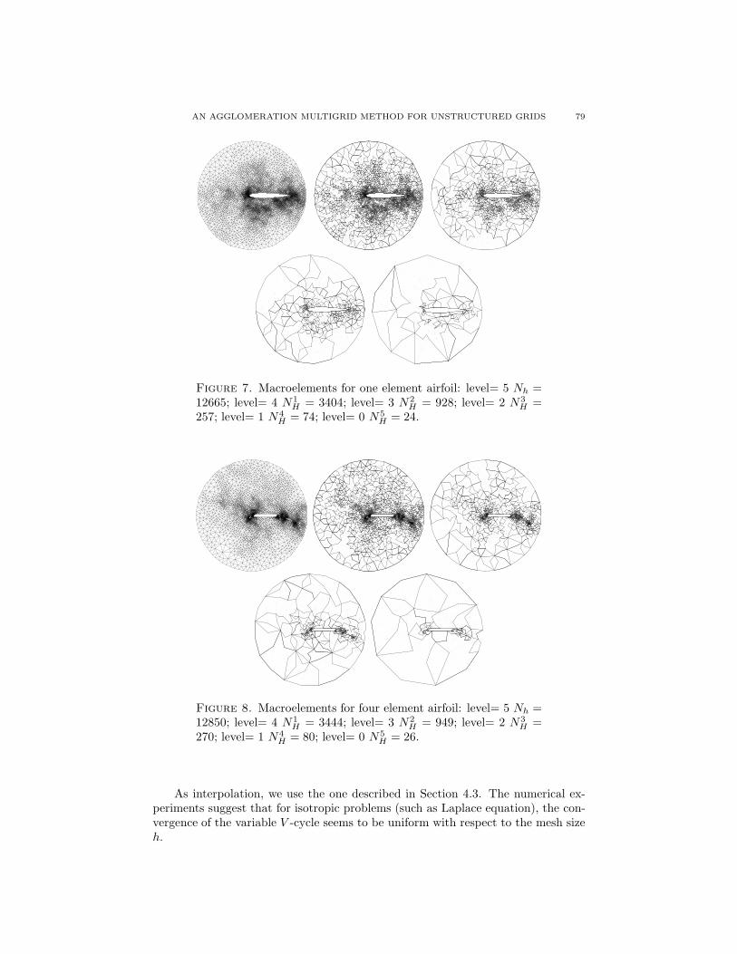
In Figures 7–8, we plot the macroelements for different unstructured grids anddifferent number of levels to illustrate the coarsening algorithm. These fine gridsare obtained by Delaunay triangulation of randomly placed point sets. They arenot obtained by any refinement procedure. Figure 9 shows the convergence historiesfor a varying number of unknowns on two types of grids. One of these (one-elementairfoil) has one internal boundary, the other one has four internal boundaries.


Figure 7. Macroelements for one element airfoil: level= 5 Nh =12665; level= 4 N1

H = 3404; level= 3 N2H = 928; level= 2 N3

H =257; level= 1 N4

H = 74; level= 0 N5H = 24.

Figure 8. Macroelements for four element airfoil: level= 5 Nh =12850; level= 4 N1

H = 3444; level= 3 N2H = 949; level= 2 N3

H =270; level= 1 N4

H = 80; level= 0 N5H = 26.

As interpolation, we use the one described in Section 4.3. The numerical ex-periments suggest that for isotropic problems (such as Laplace equation), the con-vergence of the variable V -cycle seems to be uniform with respect to the mesh sizeh.


1-element airfoil

nodes Reductionfactor

Nh = 72139 0.27049

Nh = 18152 0.22695

Nh = 4683 0.19406

Nh = 1315 0.15017

4-element airfoil


Nh = 72233 0.28608

Nh = 18328 0.21359

Nh = 4870 0.18889

Nh = 1502 0.14799

1 2 3 4 5 6 7 8 9 1010

−6

10−5

10−4

10−3

10−2

10−1

100

Nh = 72139

Nh = 18152

Nh = 4683

Nh = 1315

1 2 3 4 5 6 7 8 9 10 1110

−6

10−5

10−4

10−3

10−2

10−1

100

Nh = 72233

Nh = 18328

Nh = 4870

Nh = 1502

Figure 9. Convergence history and average reduction per itera-tion for varying number of unknowns, V -cycle

References

1. R. Bank and J. Xu, An algorithm for coarsening unstructured meshes, Numer. Math. 73(1996), no. 1, 1–36.

2. D. Braess, Towards algebraic multigrid for elliptic problems of second order, Computing 55(1995), 379–393.

3. J. Bramble, Multigrid methods, Pitman, Notes on Mathematics, 1994.4. James H. Bramble, Joseph E. Pasciak, Junping Wang, and Jinchao Xu, Convergence estimates

for multigrid algorithms without regularity assumptions, Math. Comp. 57 (1991), no. 195, 23–45.

5. T. F. Chan and Barry Smith, Domain decomposition and multigrid methods for elliptic prob-lems on unstructured meshes, Domain Decomposition Methods in Science and Engineering,Proceedings of the Seventh International Conference on Domain Decomposition, October 27-30, 1993, The Pennsylvania State University (David Keyes and Jinchao Xu, eds.), AmericanMathematical Society, Providence, 1994, also in Electronic Transactions on Numerical Anal-ysis, v.2, (1994), pp. 171–182.

6. P. Vanek, J. Mandel, and M. Brezina, Algebraic multi-grid by smoothed aggregation for secondand forth order elliptic problems, Computing 56 (1996), 179–196.

7. P. Vanek and J. Krızkova, Two-level preconditioner with small coarse grid appropriate forunstructured meshes, Numer. Linear Algebra Appl. 3 (1996), no. 4, 255–274.

8. H. Guillard, Node-nested multi-grid method with Delaunay coarsening, Tech. Report RR-1898,

INRIA, Sophia Antipolis, France, March 1993.9. W. Hackbusch, Multi-grid methods and applications, Springer Verlag, New York, 1985.

10. W. Hackbusch and S. A. Sauter, Composite finite elements for the approximation of PDEson domains with complicated micro-structures, Numerische Mathematik 75 (1995), 447–472.


1-element airfoil


Nh = 72139 0.18255

Nh = 18152 0.16627

Nh = 4683 0.14028

Nh = 1315 0.12149

4-element airfoil


Nh = 72233 0.17827

Nh = 18328 0.14621

Nh = 4870 0.13057

Nh = 1502 0.13269

1 2 3 4 5 6 7 810

−6

10−5

10−4

10−3

10−2

10−1

100

Nh = 72139

Nh = 18152

Nh = 4683

Nh = 1315

1 2 3 4 5 6 7 810

−6

10−5

10−4

10−3

10−2

10−1

100

Nh = 72233

Nh = 18328

Nh = 4870

Nh = 1502

Figure 10. Convergence history and average reduction per itera-tion for varying number of unknowns, variable V -cycle

11. B. Koobus, M. H. Lallemand, and A. Dervieux, Unstructured volume-agglomeration MG:solution of the Poisson equation, International Journal for Numerical Methods in Fluids 18(1994), no. 1, 27–42.

12. A. A. Reusken, A multigrid method based on incomplete Gaussian elimination, Numer. LinearAlgebra Appl. 3 (1996), no. 5, 369–390.

13. J. W. Ruge and K. Stuben, Algebraic multigrid, Multigrid methods (Philadelphia, Pennsyl-

vania) (S. F. McCormick, ed.), Frontiers in applied mathematics, SIAM, 1987, pp. 73–130.14. L. R. Scott and S. Zhang, Finite element interpolation of nonsmooth functions satisfying

boundary conditions, Math. Comp. 54 (1990), 483–493.15. J. Xu, Iterative methods by space decomposition and subspace correction, SIAM Review 34

(1992), 581–613.16. J. Xu, The auxiliary space method and optimal multigrid preconditioning techniques for un-

structured grids, Computing 56 (1996), 215–235.

Department of Mathematics, University of California at Los Angeles. 405 Hilgard

Ave, Los Angeles, CA 90024

E-mail address: [email protected]

Center for Computational Mathematics and Applications, Department of Mathe-

matics, Pennsylvania State University, State College, PA-16801


Center for Computational Mathematics and Applications, Department of Mathe-

matics, Pennsylvania State University, State College, PA-16801


an agglomeration multigrid method for unstructured grids · an agglomeration multigrid method for...

Documents