an analysis of market power in the alberta electricity market
TRANSCRIPT

University of Calgary
PRISM: University of Calgary's Digital Repository
Graduate Studies The Vault: Electronic Theses and Dissertations
2013-10-07
An Analysis of Market Power in the Alberta Electricity
Market
Kendall-Smith, Richard Paul
Kendall-Smith, R. P. (2013). An Analysis of Market Power in the Alberta Electricity Market
(Unpublished master's thesis). University of Calgary, Calgary, AB. doi:10.11575/PRISM/24831
http://hdl.handle.net/11023/1133
master thesis
University of Calgary graduate students retain copyright ownership and moral rights for their
thesis. You may use this material in any way that is permitted by the Copyright Act or through
licensing that has been assigned to the document. For uses that are not allowable under
copyright legislation or licensing, you are required to seek permission.
Downloaded from PRISM: https://prism.ucalgary.ca

UNIVERSITY OF CALGARY
An Analysis of Market Power in the Alberta Electricity Market
by
Richard Paul Kendall-Smith
A THESIS
SUBMITTED TO THE FACULTY OF GRADUATE STUDIES
IN PARTIAL FULFILMENT OF THE REQUIREMENTS FOR THE
DEGREE OF MASTER OF ARTS
DEPARTMENT OF ECONOMICS
CALGARY, ALBERTA
SEPTEMBER, 2013
© Richard Paul Kendall-Smith 2013

ii
Abstract
The thesis analyzes the ability of suppliers to influence the price of electricity in Alberta. To do
this, the thesis develops two structural measures of market power using data on hourly offer
curves and market clearing quantities from the Alberta wholesale electricity market over the
period September 1st 2009 to June 30th 2012. These market power measures quantify the ability
that the larger generating companies in Alberta had to influence the market price in each hour,
and are used by the thesis to characterize the nature of competition within the Alberta wholesale
electricity market. The structural measures of market power are also used in a regression
analysis to show how the larger generating companies in the market changed their offer
behaviour as their ability to exercise market power varied.

iii
Acknowledgements
First and foremost I would like to thank my supervisor Dr. Jeffrey Church for his consistent
guidance and feedback throughout my degree. My appreciation also goes to the contributors of
the Stephen G. Peitchinis Memorial Graduate Recruitment Scholarship and the John M.
Dalgarno Award for helping to fund my education at the University of Calgary. Additionally, I
would like to express my appreciation to Dr. Matt Ayres for helping me to understand the
nuances of Alberta’s deregulated electricity market. Finally, I would like to thank my friends
and family for their encouragement throughout this degree and Sara for her constant support.

iv
Table of Contents
Abstract ........................................................................................................................................... ii
Acknowledgements ........................................................................................................................ iii
Table of Contents ........................................................................................................................... iv
List of Tables ................................................................................................................................ vii
List of Figures .............................................................................................................................. viii
Introduction ..................................................................................................................................... 1
Chapter 1: Electricity, Market Power and Economic Efficiency .................................................... 9
1.1 Electricity Basics ................................................................................................................... 9
1.2 From a Natural Monopoly to a Competitive Market........................................................... 18
1.3 What is Market Power? ....................................................................................................... 24
1.4 Market Power in Wholesale Electricity Markets ............................................................... 28
1.4.1 Demand-Side Substitution ........................................................................................... 29
1.4.2 Supply-Side Substitution ............................................................................................. 31
1.4.3 Long-Run Considerations ............................................................................................ 32
1.5 Market Power and Economic Efficiency ........................................................................... 33
Chapter 2: The History of Alberta’s Electricity Market .............................................................. 37
2.1 The Regulated Market and the Motivations for Deregulation ........................................... 37
2.2 The Electric Utilities Act (1995) and Legislated Hedges .................................................. 40
2.3 The Electric Utilities Act (1998) and Power Purchase Arrangements ............................... 41
2.4 The Electric Utilities Act (2003) and the Alberta Utilities Commission Act (2007) ......... 47
2.5 Recent ISO Rule Developments ......................................................................................... 49
2.5.1 ‘T-2’ and Must Offer Rules ......................................................................................... 50
2.5.2 Transmission Must Run and Dispatch Down Service ................................................. 51
2.8 Generation and Ownership Changes (2000 – 2012) .......................................................... 54
Chapter 3: Alberta’s Electricity Market Structure and Fundamentals ......................................... 62
3.1 Alberta’s ‘Energy-Only’ Market Design............................................................................ 62
3.2 The Operation of Alberta’s Wholesale Electricity Market ................................................ 64
3.3 The Supply and Demand for Electricity in Alberta............................................................ 66
3.3.1 Market Demand Fundamentals .................................................................................... 66
3.3.2 Market Supply Fundamentals ...................................................................................... 74
v
3.4 Control over Generation Capacity...................................................................................... 83
3.5 Information Availability ..................................................................................................... 88
Chapter 4: Literature Review –Market Power in Deregulated Electricity Markets..................... 89
4.1 Market Concentration Measures and ‘the Relevant Market’ ............................................. 90
4.2 The Residual Suppler Index ............................................................................................... 97
4.3 Residual Demand Analysis .............................................................................................. 107
4.4 The Lerner Index and Offer-Cost Margins ...................................................................... 120
4.5 Net Revenue Analysis ...................................................................................................... 123
4.6 Output Gap Analysis ........................................................................................................ 124
4.8 Competitive Market Simulations ..................................................................................... 128
Chapter 5: Measures of Market Power for the Alberta Wholesale Electricity Market .............. 133
5.1 Residual Demand Analysis .............................................................................................. 133
5.1.1 Residual Demand Analysis: Economic Underpinnings ............................................ 133
5.1.2 Residual Demand Analysis: Empirical Estimation ................................................... 138
5.2 The Adjusted RSI ............................................................................................................. 147
5.2.1 RSI Measures: Economic Underpinnings .................................................................. 147
5.2.2 The Importance of ‘Must-Run’ Generation in Alberta .............................................. 154
5.2.3 Adjusted RSI: Empirical Estimation ......................................................................... 157
5.3 Additional Considerations - Incentives and Expectations................................................ 162
5.3.1 Ability vs. Incentives ................................................................................................. 162
5.3.2 Factors which Influence the Incentives of Generators in Alberta ............................. 165
5.3.3 Generator Expectations .............................................................................................. 171
Chapter 6: Empirical Results and Analysis ............................................................................... 173
6.1 Market Power Estimates Over Time ................................................................................ 173
6.2 The Distribution of Market Power ................................................................................... 177
6.3 Alberta Electricity Prices, Market Fundamentals and Market Power .............................. 183
6.3.1 The Distribution of Electricity Prices in Alberta ....................................................... 183
6.3.2 Pool Prices, Market Demand and the Price of Natural Gas....................................... 185
6.3.3 Pool Prices and Structural Market Power .................................................................. 191
6.3 Structural Market Power and Supplier Offer Behaviour .................................................. 196
6.3.1 ENMAX – Background and Quantitative Analysis .................................................. 196

vi
6.3.2 TransCanada – Background and Quantitative Analysis ............................................ 201
6.3.3 Econometric Analysis: Setup ..................................................................................... 204
6.3.4 Econometric Analysis: Results .................................................................................. 211
6.4 The Impact of Market Events on Firm Offer Behaviour .................................................. 218
6.4.1 The OBEGs: Relevant Background ........................................................................... 218
6.4.2 The OBEGs: Econometric Analysis .......................................................................... 222
6.5 Broader Implications (a simple Counterfactual Analysis) ............................................... 228
Bibliography ............................................................................................................................ 238
Academic References .......................................................................................................... 238
Industry References ............................................................................................................. 241

vii
List of Tables
Table 1: PPAs – Capacity, Retirements and Term Dates ............................................................. 43 Table 2: An example of the DDS Market (January 6th 2011 HE 12)............................................ 53 Table 3: The offer curve submitted for Sheerness #1 (August 5th 2012 from 6pm to 7pm) ........ 65 Table 4: Alberta Internal Load by sector in 2010 (Source AESO Long-Term Transmission Plan 2012). ............................................................................................................................................ 69 Table 5: Alberta Capacity by Fuel (Source AESO CSD page Aug 2013).................................... 74 Table 6: The Available Capacity on Alberta’s Interties (Jan 2010 – Sep 2012) .......................... 83 Table 7: Thermal Units that remain under Power Purchase Arrangements.................................. 86 Table 8: Long-term contractual obligations are common at co-generation assets in Alberta ...... 87 Table 9: The distribution of the Residual Demand estimates - Summary Statistics ................... 178 Table 10: The Percentage of hours in which generators had an Inverse Adjusted RSI above a certain level ................................................................................................................................. 180 Table 11: ENMAX’s Alberta generation portfolio ..................................................................... 198 Table 12: TransCanada’s generation portfolio in Alberta .......................................................... 203 Table 13: The Adjusted RSI grouped analysis .......................................................................... 208 Table 14: Econometric Results for the Adjusted RSI Analysis .................................................. 212 Table 15: Econometric Results for the Residual Demand Analysis ........................................... 212 Table 16: The Econometric Results for the Adjusted RSI Grouped Analysis (ENMAX units) . 213 Table 17: The Econometric Results for the Adjusted RSI Grouped Analysis (TransCanada units)..................................................................................................................................................... 214 Table 18: The Econometric Results for the Cloverbar facility ................................................... 215 Table 19: Econometric Results pre and post OBEGs for various units ...................................... 223 Table 20: The impact of the OBEGs and the EPCOR RRO on Cloverbar’s offer behaviour .... 228 Table 21: The Contribution of Adjusted RSI groups to the Average Prices in 2011 ................. 236

viii
List of Figures
Figure 1: Map of North American Electricity Jurisdictions (2008) .............................................. 14 Figure 2: Marginal Revenue – the inframarginal gain vs. the marginal loss ................................ 26 Figure 3: Cogeneration and Wind have increased their relative capacity since deregulation ..... 54 Figure 4: Annual Generation Additions and Retirements by fuel type (2000 – Q2 2012) ........... 55 Figure 5: Uprates have added a total of 1,140 MW since 2000 .................................................... 56 Figure 6: The Annual market shares of today’s largest five firms (2000-2012) .......................... 57 Figure 7: The average demand of ‘Price Responsive Loads’ at $50 price intervals.................... 68 Figure 8: The Average hourly Load Shape in Alberta ................................................................. 70 Figure 9: The hourly Load profile in Alberta varies across seasons............................................ 71 Figure 10: Prevailing weather conditions play an important role in the demand for electricity . 72 Figure 11: Demand for electricity is higher during the week ...................................................... 73 Figure 12: A graphical example of the Energy Market Merit Order in January 2011 ................. 75 Figure 13: Market Share Estimates of Alberta’s generation capacity .......................................... 84 Figure 14: Many of the generation assets in Alberta have a number of Owners ......................... 85 Figure 15: Energy Market Fundamentals and the Construction of a Firm’s Residual Demand Curve ........................................................................................................................................... 139 Figure 16: The Residual Demand Function and the Offer Curve ............................................... 140 Figure 17: Example 1 - Estimating the Slope of a firm’s Residual Demand function ............... 144 Figure 18: Example 2 – Estimating the Slope of a firm’s Residual Demand function ............... 146 Figure 19: Example 1 - A firm’s Residual Demand function shows the extent to which the firm is pivotal ......................................................................................................................................... 150 Figure 20: Example 2 – A firm’s Residual Demand function shows the extent to which the firm is pivotal ...................................................................................................................................... 150 Figure 21: Two Residual Demand functions - the firm is shown to be a pivotal supplier in both cases ............................................................................................................................................ 151 Figure 22: The Impact of Fixed-Price Sales on a Generator’s Incentives ................................. 164 Figure 23: Pool Price exposure and Availability Incentive Payments an example ................... 169 Figure 24: A Simple Example of Expected Profit-Maximization .............................................. 172 Figure 25: Monthly Averages of Residual Demand Estimates ................................................... 173 Figure 26: 10-day Moving Averages of the Maximum Daily Adjusted RSI .............................. 175 Figure 27: 10-day Moving Averages of the Maximum Daily Adjusted RSI .............................. 175 Figure 28: The distribution of the Residual Demand metric for ENMAX and TransCanada .... 178 Figure 29: The Mean and Median of the Residual Demand Analysis for ATCO during peak hours ............................................................................................................................................ 179 Figure 30: The Mean and Median of the Residual Demand Analysis for TransCanada during peak hours ................................................................................................................................... 179 Figure 31: The distribution of the Adjusted RSI measure for the 5 largest generators in Alberta..................................................................................................................................................... 180

ix
Figure 32: The distribution of the Residual Demand estimates across weekday hours for ENMAX and TransCanada ......................................................................................................... 181 Figure 33: The distribution of TransCanada’s Adjusted RSI across weekday hours ................ 182 Figure 34: The Distribution of Hourly Pool Prices over the sample period .............................. 183 Figure 35: The Value that 5 percentile groups made to the resulting Average Pool Price ......... 184 Figure 36: A scatterplot of Pool Prices against hourly demand in the Energy Merit Order ....... 186 Figure 37: Daily Average Pool Prices and Peak Energy Merit Order demand over the sample period .......................................................................................................................................... 187 Figure 38: There was relatively little correlation between Pool Prices and Gas Prices in the sample period .............................................................................................................................. 188 Figure 39: The Alberta market Heat Rate is heavily influenced by a few hours when electricity prices are high ............................................................................................................................. 190 Figure 40: The relationship between the hourly Pool Price and the hourly ‘Market’ Adjusted RSI..................................................................................................................................................... 192 Figure 41: The Daily Average Pool Price and the Daily Average ‘Market’ Adjusted RSI ........ 193 Figure 42: ENMAX’s Monthly Average Residual Demand estimates and Monthly Average Pool Prices ........................................................................................................................................... 195 Figure 43: Capital Power’s Residual Demand estimates and Pool Prices over time .................. 195 Figure 44: The Max. Daily Values of ENMAX’s Market Power and the Marginal Offer Price on its coal units ................................................................................................................................ 199 Figure 45: ENMAX’s market power and the dispatched Heat Rates on its Gas Assets ............. 200 Figure 46: TransCanada’s market power and the dispatched offer prices on Sheerness and Sun. B..................................................................................................................................................... 204 Figure 47: TransCanada’s market power and the marginal offer price on Sheerness ................ 209 Figure 48: The Average Marginal Offer Price on Sheerness at different levels of market power..................................................................................................................................................... 225 Figure 49: The Average Marginal Offer Price on Genesee #3 at different levels of market power..................................................................................................................................................... 226 Figure 50: The Average Marginal Offered Heat Rate on Crossfield at different levels of market power........................................................................................................................................... 227 Figure 51: Realized and Counterfactual Price Distribution Curves ............................................ 234 Figure 52: The Realized and Counterfactual Price Distribution Curves (80th percentile and up)..................................................................................................................................................... 234 Figure 53: The Contribution of Adjusted RSI groups to the Average Observed and Counterfactual Prices .................................................................................................................. 235

1
Introduction
The objective of the thesis is to analyze the extent to which the larger generators in Alberta are
able to exercise market power in the wholesale market for electricity. Market power is defined
as the ability of a supplier to influence market clearing prices. Generator market power in
wholesale markets for electricity has been, and will continue to be, an important topic for those
who design and monitor the functioning of deregulated electricity markets. Market power is a
subject of particular importance in deregulated electricity markets because these markets are
especially susceptible to being influenced by the strategic behaviour of larger generating
companies. Electricity, and the network on which it is transmitted, possess unique characteristics
that differentiate electricity from most other products, and which enhance the ability of
generators to exercise market power.
From an economic perspective, the exercise of market power is important because it can distort
market outcomes away from the efficient outcomes of a competitive market. For example, the
exercise of market power can mean that electricity for which a buyer’s willingness to pay
exceeds the variable costs of production is not produced. This results in a ‘deadweight loss’ to
society. In addition, the exercise of market power can cause high cost generators to be supplying
the market when cheaper alternatives are available, particularly when the cheaper generation is
being withheld from the market to increase price.
The exercise of supplier market power in wholesale electricity markets also has the potential to
cause significant transfers of wealth from consumers to producers in a relatively short space of
time. In hours when the exercise of market power increases the price of electricity, consumers

2
buying from the wholesale market will pay more than they would have done under a competitive
marketplace.
It is important to clarify at the outset that the exercise of market power in Alberta’s electricity
market is a lawful and rational exploitation of the ability and incentives available to the
generators. The market design, structure, and rules of engagement in Alberta’s electricity market
are such that the larger generators are able to exercise market power under certain conditions.
The distinguishing feature of the Alberta market compared to most other deregulated electricity
markets is that it is ‘energy only’. The term energy only refers to the fact that generators in the
Alberta market will only receive payments for the electricity that they supply onto the grid.
Under this market framework generators must recover all of the costs associated with supplying
electricity through their energy revenues. Therefore, under Alberta’s market framework,
generators require some degree of market power to recover the fixed costs associated with
supplying electricity.
The fundamental premise behind the Alberta market design is that competitive forces will
effectively regulate the market power of generating companies. In this way, the design of
Alberta’s electricity market is like many other deregulated markets and implicitly relies on the
generation sector being sufficiently competitive. That is, the Alberta market design requires that
prices are high enough to incentivise efficient generation investments if they are required.
However, at the same time, the sustainability of the market requires that market outcomes are not
exclusively determined by the actions of a few large generating firms. Consequently, the design
of Alberta’s electricity market means that measuring and monitoring the extent of generator
market power is a subject of great importance to the industry.
3
The thesis uses data on hourly offer curves and market clearing quantities from the Alberta
wholesale electricity market over the period September 1st 2009 to June 30th 2012 to develop two
structural measures of market power. These market power measures quantify the ability that the
larger generating companies in Alberta had to influence the market price in each hour. These
market power measures are then used to characterize the nature of competition within the
market.
The two structural measures of market power both use realized market supply and demand
fundamentals to estimate the market power that each of the larger generators had in a particular
hour. The first metric analyzes the offers submitted by competiting generators around the market
clearing price to estimate the extent to which these offers limited the firm’s ability to influence
price. The second approach estimates how pivotal a generator’s priced1 offers were to the
clearing of the market. The intuition here is straightforward, the more a firm’s priced generation
was needed by the market, the more influence these offers were deemed to have had on the
market price.
The resulting quantitative evidence strongly suggests that each of the larger generators in Alberta
had the ability to exercise significant levels of market power during a small percentage of hours
within the sample period. The ability of suppliers to exercise market power during these hours
was often driven by a combination of high market demand and a number of baseload coal-fired
units being offline. The pool prices observed during these hours were frequently very high and,
whilst these periods represented a small subset of the total number of hours, their impact on the
prevailing average market price was notable. The average price during the sample period was
1 ‘Priced’ here means offered into the market above $0.

4
$60/MWh but if the top 5% of hours are excluded, the average price in the remaining hours was
only $33/MWh. In summary, the thesis shows that average prices for electricity in Alberta are
driven by relatively few hours, and in these hours the market fundamentals illustrate that the
larger generators in the province had a meaningful ability to influence the market clearing price.
Therefore, the thesis illustrates a strong degree of correlation between market prices and the
prevailing level of market power possessed by the larger generators.
That said, the two market power measures also indicate that in a large percentage of hours the
ability of the larger generators in Alberta to influence market outcomes was actually quite
limited. In many hours, Alberta’s demand for electricity was too low or the level of competing
generation was too high for the larger firms to materially influence price unilaterally. This
distribution of competition is also evident in the distribution of electricity prices across the
sample period. In most hours the price of electricity in Alberta is quite low, and almost 90% of
the hours within the sample period fell below the average pool price of $60/MWh. In addition,
for the vast majority of hours, the hourly price for electricity is highly correlated with the
prevailing price of natural gas in the province. The conclusion here is that in most hours the
Alberta electricity market is competitive.
The thesis also examines whether the two largest generating companies in Alberta (ENMAX and
TransCanada) exercised their market power by offering their generation output into the
wholesale market at prices above what they would have offered under competitive conditions. In
particular, the thesis uses an econometric analysis to quantify how the offer behaviour of the two
largest suppliers in the Alberta electricity market changed as their ability to exercise market
power varied over the sample period. The thesis uses regression analysis to show that, after

5
controlling for input fossil fuel prices and other factors that influence the costs of producing
electricity, some of the generating units belonging to these larger firms submitted a higher offer
price when the firm had a greater ability to exercise market power, whilst other units did not. In
summary, it is shown that the offer strategies employed on TransCanada’s coal-fired generating
units were very responsive to changes in the firm’s ability to exercise market power. As the
firm’s ability to exercise market power increased, TransCanada offered its capacity into the
market at higher prices. In contrast, the offer prices on ENMAX’s coal-fired units were almost
entirely unresponsive to changes in its ability to influence price. In terms of ENMAX’s gas-fired
units, the regression results show that these units were sometimes offered at a higher price when
ENMAX had a higher ability to exercise market power.
This econometrics approach is also used to analyze the impact that the Offer Behaviour
Enforcement Guidelines (OBEGs) had on the conduct of suppliers in the Alberta wholesale
electricity market. Towards the end of 2010, Alberta’s Market Surveillance Administrator
(MSA) clarified to stakeholders that a unilateral exercise of market power was not deemed to be
anti-competitive conduct. Prior to the MSA’s consultation process, the rules surrounding
unilateral exercises of market power were not completely clear, for instance previous
Independent System Operator (ISO) rules specified that “When a market participant in a
dominant position exploits its market power in a way that adversely impacts upon the efficient,
fair and openly competitive operation of the market, it will be considered an abuse of
dominance.”
By separating the sample period into pre- and post-OBEGs eras, the econometric models were
re-estimated and a test of significance was used to see whether or not any changes in conduct had

6
occurred. Almost all of the units analyzed showed a significant change in the extent to which
their offer prices varied with the level of market power held by the controlling firm. The
regression results show that units controlled by TransCanada, TransAlta and Capital Power all
increased their responsiveness to changes in their ability to exercise market power after the
OBEGs. This observed change was most notable in the few hours when these generators had a
significant level of market power. The implication is that prior to the OBEGs these firms were
being somewhat ‘reserved’ in their offer strategies during these hours. In contrast, the offer
prices submitted on ENMAX’s gas units actually became less responsive to the firm’s ability to
exercise market power after the OBEGs. One potential explanation for this is that consumers
may have purchased more fixed-price power through ENMAX’s retail arm in response to the
offer behaviour observed after the OBEGs. The increase in the level of fixed-price sales would
in turn reduce ENMAX’s incentives to exercise market power.
These empirical results lead to the following conclusions about the behaviour of the larger
suppliers in the Alberta electricity market. Firstly, some of these generators are successful at
increasing market clearing prices by raising their offer prices into the wholesale market when
they have a greater ability to exercise market power. Secondly, the results indicate that the level
of forward contracting has a significant effect on the conduct of the larger firms in the Alberta
wholesale market. ENMAX, one of the largest generators in the province, also has a significant
presence in the retail market and sells a large amount of its generation at fixed prices. As a
result, ENMAX’s offer prices are generally less responsive to changes in its ability to exercise
market power when compared with the responsiveness of ‘merchant’ generating companies in
the market. Finally, the econometric results imply that the OBEGs did have a meaningful
influence on the conduct of the larger generators in Alberta. The major change here is that these
7
suppliers are now less reserved with the offer strategies that are employed when their ability to
exercise market power is notably high.
To obtain a broad sense of the price implications resulting from the exercise of unilateral market
power in the Alberta wholesale electricity market, the thesis undertakes a simple counterfactual
analysis for the year 2011. In the counterfactual analysis TransCanada’s Sundance B and
Sheerness assets are offered into the market as if the firm had little to no market power. To do
this, hours when TransCanada’s ability to exercise market power was shown to be limited were
used to estimate a ‘competitive’ offer price for these units. The counterfactual analysis takes any
unusually high offer prices on the Sundance B and Sheerness units and reduces them to this
competitive level. Everything else in the market is left unchanged and a counterfactual price is
calculated. The results of this simple counterfactual analysis show that with these coal units
TransCanada’s influence on the market clearing prices was high. The average price observed in
2011 was $76. However putting the Sundance B and Sheerness units at competitive offer prices
yields an average annual price of $52. The results of the counterfactual analysis are consistent
with the intuition derived above. In the vast majority of hours, the counterfactual prices
calculated were very close to the prices that were observed in the market, implying TransCanada
did not offer strategically with the units, or its price impact of doing so was minimal. However,
in the few hours that TransCanada’s pricing strategies did have a price impact, it was sometimes
very significant.
The remainder of the thesis proceeds as follows. In Chapter 1 the thesis will provide a broad
explanation of electricity markets and market power, and why the unique properties of electricity
mean that the exercise supplier market power is of particular concern in these markets. Chapter

8
1 will also outline the general motivations behind the deregulation of electricity markets.
Additionally, Chapter 1 will discuss the economic implications of market power being exercised.
Chapter 2 provides a history of the deregulation process undertaken in Alberta, explaining why
the market was deregulated and how this process has been undertaken. Chapter 3 details how the
Alberta wholesale electricity market operates and explains why the ‘energy only’ market design
is an important consideration. Chapter 3 also discusses the supply and demand fundamentals in
Alberta, explaining why and how these dynamic market fundamentals change to influence the
extent of competition in the wholesale market. Chapter 4 then provides a review of the literature
surrounding the subject of measuring market power in electricity markets. This review explains
the variety of measures that have been used to analyze supplier market power in electricity
markets, and outlines some of the benefits and drawbacks associated with each method. Chapter
5 details the two measures of market power that are used in the thesis. In particular, Chapter 5
outlines the economic rationale underpinning each of the two measures, and also explains how
the measures are calculated using publicly available data from the Alberta Electric System
Operator (AESO). Chapter 6 reports the results of the thesis, explaining how the market power
of firms varied over the sample period and analyzing the distribution of generator market power
within the sample. Chapter 6 also highlights the correlation between supplier market power and
market prices. Chapter 6 then explains and reports the results of econometric approaches, which
are used to highlight the relationship between generator offer behaviour and market power.
Finally, Chapter 6 undertakes a simple counterfactual analysis to illustrate the observed impact
of a single generator’s market power on the price for electrcity in 2011.

9
Chapter 1: Electricity, Market Power and Economic Efficiency
1.1 Electricity Basics
The supply of electricity can usefully be broken down into four sectors: generation, transmission,
distribution and retailing. The generation (or wholesale) sector refers to the production of
electrical power using various forms of energy. Power stations create electricity by using
mechanical energy to turn a turbine, which spins large amounts of copper wire between huge
magnets at very high speeds. When a magnetic field is in motion relative to a copper wire it
triggers the flow of electrons in the wire, thus creating electricity. Steam turbine generators, gas
turbine generators, diesel engine generators and nuclear power all follow this principle, each
providing a unique way to spin the copper wiring.2 Therefore, electricity can be generated in a
variety of ways. A common example is the use of pressurized steam to turn the turbines, since
the required steam can be produced by burning fossil fuels (predominantly coal and natural gas),
via nuclear fission, or by using renewable technologies such as biomass or thermal energy.
Electricity can also be generated by turning turbines directly through burning natural gas, using
falling water, or with wind energy.
The transmission of electrical energy refers to the transfer of electricity from generation sites to
electrical substations located near local distribution centers. Voltage is the amount of electrical
pressure that pushes the electrical current across the network, and this pressure is measured in
2 The Electricity Forum website – How Electricity is Generated. The major exception to this principal is the use of
solar panels, which generate electricity by converting solar radiation into direct current electricity using
semiconductors.

10
volts (Stoft (2002)). The transmission of electricity involves the use of over-head power lines3,
transformers and substations to transmit power at high-voltages (generally 110 Kilovolts (kV)
and above). High-voltages are used to reduce the energy losses4 associated with transmitting
electricity over long-distances.
From the transmission network, the power flows into the distribution networks which are used to
deliver electricity to consumers. The transmission network and distribution network are linked
by substations where the voltage is lowered to a level that can be used in homes and businesses.
The distribution network carries electricity at low-voltages from the nearby substations to the
end consumer.5 Typically, distribution networks would include power lines of less than 50 kV,
substations, pole-mounted transformers, and additional lower-voltage wiring. The target
residential voltage in Canada and the United States is 120 volts.
The retail sector of the electricity industry is responsible for metering and billing consumers for
their electricity use. A primary function of the retailing sector is to manage the risks associated
with buying power from the wholesale sector by selling electricity to consumers at fixed prices.
Electricity retailers can purchase power from the real-time ‘spot’ market or through long-term
financial contracts and derivatives. Some vertically-integrated companies operate in both the
retail and the generation sectors and generate a substantial portion of their retail sales
themselves. Consumers in deregulated electricity markets can choose from a variety of
3 Power can also be transmitted using underground power lines in urban or sensitive areas, although underground
lines are significantly higher cost and also have greater operational limitations. 4 Losses refer to the electrical energy that is consumed by the network. 5 AltaLink website – Electricity at a Glance.

11
electricity price products – from 5-year fixed rates all the way to wholesale or ‘flow through’
pricing.6
While the basic structure of the electrical sector (wholesale, transportation and marketing) is
comparable with other commodity markets, electricity has physical characteristics which mean
that electricity markets are unique in important ways.
Maintaining Frequency: Supply = Demand
Electrical energy is a homogenous good that is injected into the transmission grid by all
generators and is withdrawn by all end users. There is usually no way to identify the electricity
generated by producer A with the power utilized by consumer B. A useful analogy is to think of
the transmission grid as a large pond, with producers putting water into the pond while
consumers are simultaneously taking water out (Griffin and Puller (2005)).
In addition, the characteristics of the delivered electricity must be uniform and carefully
maintained. Power systems attempt to maintain a constant frequency, the rate at which alternate
current alternates (Stoft (2002)). In North America power systems are operated at a frequency of
60 Hz. To deliver power at a certain frequency requires the generator to be synched with the
grid and rotating their turbines at a certain rate. To maintain the overall frequency of the grid
requires that the supply of power matches the consumption of power at every point in time. To
continue with the above analogy, it is as if the amount of water being added and removed from
the pond must always be the same, so that the level of the pond remains constant. If the
consumption of electricity exceeds the amount being generated at any point in time, the electrical
6 The Utilities Consumers Advocate website lists the range of retail contracts that are available in Alberta.

12
frequency on the grid will fall. If the frequency drops too much, generators and loads can
automitically trip offline to prevent damaging their equiptment, and at this point the system
controller loses all control over the grid. To prevent this, the system controller will shed load in
the event of a supply shortfall, with the result being that a large number of consumers may be
‘blacked-out’. On the other hand, if the supply of electricity exceeds the level of consumption at
any point in time, the electrical frequency will increase, which has the potential to be severely
dangerous and to substantially damage equipment connected to the grid. Therefore, unlike many
other goods, electricity cannot be readily disposed of when the market is over-supplied, and if
the grid is slightly under-supplied large areas of the market can lose the ability to consume
power.
Because supply and demand imbalances have the potential to disrupt the entire electrical
network, a System Operator is needed to coordinate schedules of generation, consumption and
power flow and balance deviations from expected supply and demand. In effect, Adam Smith’s
invisible hand is hardly invisible for electricity markets (Griffin and Puller (2005)). The
precarious need to balance supply and consumption on electrical networks also means that there
is a vast amount of readily-accessible data in these markets. For example, the market supply
curve for electricity in Alberta for a given hour is readily available on the AESO website. This
supply curve shows the prices at which each generator in the province was willing to sell its
electricity in that hour. This is in stark contrast to many other markets, where it is often difficult
to get an accurate idea of market-clearing prices and quantities.
Maintaining the reliability of electrical networks is a non-trivial task since electricity demand is
relatively volatile, changing significantly from one hour to the next as consumers go about their

13
daily routines, as weather conditions vary, or as large industrial loads alter their power demands.
As a result, the aggregate demand for power will routinely vary by 50% over a single day in
some jurisdictions (Griffin and Puller (2005)). In addition, the demand for power is not
responsive to changes in price and electricity is prohibitively expensive to store. The overriding
economic implication of these factors is that electricity markets are distinguished by time, so
electricity produced at 5am may have a significantly different value to electricity produced three
hours later.
These factors also mean that the need to continuously balance supply and demand requires a
complex monitoring and control mechanism. An important aspect of this control mechanism is
for the market to provide a range of services to ensure adequate reserve capacity so that the lights
stay on in the event of unanticipated shocks to the market. A major way for electricity markets
to manage disparities between supply and demand is through interconnections with other
jurisdictions. For example, when a large coal unit trips offline unexpectedly in Alberta, the flow
of electricity from British Columbia into Alberta will naturally increase. The electricity network
in BC is itself connected to the Pacific Northwest and, in turn, to markets in California - these
markets are all part of the Western Electricity Coordinating Council (WECC) area (see figure 1).
Through the interties, jurisdictions can share the burden (and costs) of reliability. However,
there are various ‘good neighbour’ policies and each jurisdiction is expected to alleviate its own
reliability issues reasonably promptly.

14
Figure 1: Map of North American Electricity Jurisdictions (2008)
Therefore, each jurisdiction must procure enough reserve capacity to maintain system balance in
the event of a large unexpected outage, or a surprising change in market demand. To do this, the
system operator must also run a market through which generating and load facilities are paid to
provide a variety of network support services. In Alberta these support services are procured by
the Alberta Electric System Operator (‘AESO’) through the Ancillary Services (‘AS’) market.7
Kirschoffs Laws: The relationship between Generation and Transmission
The operation of electricity markets is further complicated by the fact that the location of
generators and consumers is important. A local distribution company will withdraw electricity
from the transmission grid at specific locations, and generators will inject electricity at specific
7 The AESO’s Ancillary Services participants manual provides a great amount of detail on the reserve products and
services that are procured in Alberta.

15
locations. The ‘transportation system’ for electricity is more complex that in other commodity
markets, such as oil or natural gas, because electricity cannot simply be sent from a generator at
point A, along transmission line X, to be delivered at point B. Instead, electricity will flow along
a transmission line in accordance with Kirchoff’s laws, which dictate that power will flow along
the transmission network according to the path of least resistance. Therefore, an injection or
withdrawal of electricity at any one point on the transmission system will impact the system at
every other point (Stoft (2002)). These network externalities have important consequences for
the efficient operation of the market and the optimal investments in generation and transmission.
Short-run Implications: Congestion and Line Losses
The efficient operation of the electrical system at any point in time requires using the lowest cost
generation to meet the market’s demand. However, the use of a particular generator may be
constrained, or the costs of using that generator may be materially influenced, by the prevailing
conditions on the transmission network.
Transmission lines have a finite capacity and only a certain amount of power can flow along a
particular transmission path. When this capacity is reached it prevents generation flowing from
one area to meet the prevailing level of consumption in another, and the market is said to be
congested. In this event, generation within the congested area cannot be used to service the load
outside of the congested area, and generation outside of the congested area is required.
Congestion on the grid will influence both the value of electricity, since power outside the
congested area will be of more value, and the level of competition, because the ability of
generation capacity in the congested to compete is limited.

16
In addition to congestion, the location of generation and loads on the transmission grid will also
play an important role in determining the amount of electricity energy that is lost its
transmission. The extent of these ‘line losses’ will depend on a number of factors but will fall as
more transmission capacity is available and as the distance travelled is reduced. Therefore, the
location of generators on the transmission grid can play an important role in determining their
overall costs, as greater line losses will increase the costs of the power.
Long-run Implications: Investment Decisions
Given the preceding discussion, it is clear that there is an important relationship between
investments in transmission and investments in generation. As outlined above, the ability of
generators to get their product to market is influenced by their location and the strength of the
transmission network. Therefore, investments in generation will be influenced by the
interconnections provided by (or planned to be provided by) the transmission system.
Conversely, the location and the amount of generation that is built will affect where and how
much transmission capacity is required. Although it is clear that in the short-run the relationship
between transmission and generation is complimentary8, the long-run relationship may be
viewed as one of substitutes; the development of generation in a City may offset the need for
transmission developments to bring in power from elsewhere, whilst the development of
transmission capacity in the area may offset the need for local generation.
8 Greater transmission capacity within an area will mean that local generators are unconstrained and will also serve
to reduce their line losses.

17
Generation Characteristics
Since electrical energy can be generated in a variety of ways, it is unsurprising that the supply-
side of electricity markets is characterized by a wide array of production processes. As a result,
suppliers of power will not face a uniform cost structure but instead generating assets will have a
wide range of marginal, fixed and sunk costs. For example, coal-fired generation has high fixed
and sunk costs but relatively low variable productions costs, whereas peaking gas-fired units
have high variable costs but are relatively cheap to build. Because of these cost differences
electrical supply functions are not continuous and there can be large price gaps between the
prevailing market supply and the price at which additional capacity is available.
An important constraint on the supply-side is that electricity is prohibitively expensive to store.
Unlike commodities such as oil and natural gas, the technologies for electricity storage which are
currently available, including large industrial batteries and hydroelectric pump storage, are
relatively inefficient (i.e. higher cost) in comparison with building additional peaking capacity.
In addition, all generation assets face binding capacity constraints in the short-run, strictly
limiting the total market supply available at a given point in time. In the long-run, developing
new generation capacity is a lengthy process, with short lead-time generators taking upwards of
2 years to build and requiring large capital investments. The market implication of these
characteristics is that the competition within electricity markets can vary significantly across
time. For example, the market supply function can be extremely inelastic at times of peak
demand, when many assets are fully dispatched and are unable to respond to further increases in
price.

18
Given the unique characteristics involved in the production and transmission of electrical energy,
the deregulated approach to the supply of power is necessarily distinct from other markets. In
particular, the precarious need to ensure system integrity at each point in time, the notable links
between generation and transmission, and the important network externalities in transmission, all
preclude the ability of a decentralized invisible hand to efficiently coordinate the market.
Instead, a very visible System Operator is required to constantly co-ordinate generation, load and
the instantaneous flow of power on the grid, according to strict safety and reliability
requirements (Wipond (2008)). In addition, given the variation of system load and the short-run
constraints on market supply, it is unsurprising that electricity markets can be characterized by
fairly extreme price volatility over relatively short periods of time. The unique characteristics of
electricity are important in understanding why market power remains a principal concern in
deregulated wholesale electricity markets.
1.2 From a Natural Monopoly to a Competitive Market
Prior to the 1990s North American electricity markets were typified by geographic vertically-
integrated utilities which were heavily regulated on both the prices charged to consumers and the
investments made in generation. These utilities were given exclusive rights to sell electricity to
retail consumers in specific franchise areas and were regulated on a cost-of-service basis.
Throughout Europe most electricity markets were run by state-owned utilities. The principal
economic rationale underlying these regulatory structures was that electricity markets
represented a natural monopoly. That is, a single vertically-integrated utility would be able to
produce electricity at a lower cost than a number of smaller competing suppliers:

19
“For nearly a century, the electricity sector in all countries has been thought of as a
“natural monopoly” industry, where efficient production of electricity required reliance
on public or private monopoly suppliers subject to government regulation of prices,
entry, service quality and other aspects of firm behavior.” Joskow (1997)
Griffin and Puller (2005) note that the generation, transmission and distribution sectors of
electricity markets all had natural monopoly characteristics. In generation, the economies of
scale associated with large coal-fired and nuclear plants, coupled with the localized pockets of
demand and the substantial line losses from long-distance transmission, meant that generation
was an operation efficiently undertaken by a single utility. Similarly, there was, and remains, no
rationale for allowing the duplication of transmission and distribution facilities. The scale
economies in both sectors prohibit the efficiency of building multiple competing networks.
In addition to the argument of natural monopoly, many economists highlight the theory of
transaction costs in explaining the traditional regulated structure of electricity markets.
Transaction cost economics posits that one mode of governance will be chosen if it maximizes
the net gains from trade. By evolving as a market vertically integrated across generation and
transmission, utilities were able to conduct important transactions within a single firm rather than
through two firms on the market. The long lives and asset-specific nature of large, sunk
investments in generation and transmission implies that transactions between two separate
parties are susceptible to opportunistic behavior such as moral-hazard and hold-up.9 For these
reasons, the costs of negotiating and undertaking such delicate transactions can be substantial.
9 See Bacalso (2000) for an insightful and detailed discussion.

20
Through vertical integration the market aligns the incentives of the parties and is able to remove
these transaction costs.
Another principal attraction of vertical integration is the ability of a single utility to select the
supply of electricity that minimizes the total all-in costs. To do this necessitates consideration,
and coordination, of the generation and transmission sector costs. Joskow and Schmalensee
(1983) contend that the generation sector, in isolation from the transmission network, had not
been a natural monopoly market for some time. Instead, they contend that the intrinsic need to
vertically integrate the generation sector with the transmission function caused the generation
sector to be characterized as a natural monopoly as well.
While the monopolization of electricity markets does have advantages, an unregulated
monopolist would have substantial market power. To address this issue, monopoly utilities were
regulated on a cost-of-service basis, with the regulator being responsible for approving
investments and administering prices. These “bundled” prices were set to cover all operating
costs and to allow investors a fair rate-of-return on the capital invested in large sunk and fixed
costs. Effectively, prices were set to cover the average cost of supplying electricity.
Beginning with Chile in the 1980s, a growing number of countries around the world have
restructured their electricity supply industries to introduce competition into the wholesale and
retail sectors (Wolak (2010)). The motivations behind deregulation varied from one region to
another, but generally stemmed from the ability to obtain cheaper power, either from generation
built by private companies or by buying power from other jurisdictions where prices were low.
The frustrations with the existing utility structure were also given additional weight because of

21
the successful deregulation of other “natural monopoly” markets such as natural gas,
telecommunications and airlines.
In addition, technological advancements in high-voltage transmission meant that electrical
energy could be efficiently transmitted across long distances with fewer line losses. Meanwhile
new Combined Cycle Gas Turbine technology, and falling natural gas prices, meant that
generation capacity could now be built efficiently on a lower scale. Both of these advancements
undermined the arguments that electricity generation remained a natural monopoly. Finally, the
development of sophisticated computer and communications systems, which permitted the real-
time monitoring and control of electricity markets, was also an important development in
expediting the movement to deregulated wholesale markets.
Economic theory highlights the potential efficiencies to be gained by moving from a market
regulated on a cost-of-service basis to one shaped by competitive forces. In particular, the link
between prices and costs under traditional cost-of-service regulation provides weak incentives
for utilities to achieve lower costs. Church and Ware (2000) explain that if the utility is able to
lower its costs, the benefits of cost efficiency accrue to the consumers in the form of lower
prices, not to the firm in the form of higher profits. If costs increase, then so do prices, and the
firms – or more accurately, their shareholders – continue to earn a pre-specified rate-of-return.
This theory was evident in regulated American power markets as White (1996) and Joskow
(1997) highlighted that there were significant variations in performance across utilities, and yet
the regulatory structure provided limited opportunities for the efficient utilities to expand at the
expense of the inefficient suppliers. White (1996) emphasized that new entrants could build
combined-cycle generation assets with average-costs well below those of many incumbent

22
utilities. As a result there existed a price-gap between generation services embedded in the
bundled regulatory prices and the generation services that would be available to the consumers in
the wholesale market. A significant amount of this disparity could be explained by the
overbuilding of capacity and the development of inefficient generation (most notably nuclear)
with large sunk costs that had to be recovered under the regulated regime. Consequently, a large
driver behind deregulation in many US states was the potential for lower prices in competitive
markets.
“While on average real US retail electricity prices fell after 1985, in the Northeast,
California, and a few other states, real retail prices continued to rise into the late 1980s
and early 1990s as the legacy costs of nuclear plants, combined with excess generating
capacity, continued to be reflected in regulated retail prices.”
Joskow in Griffin and Puller (2005)
The unique aspects of electricity markets, however, meant that realizing productive efficiencies
in the short-run from deregulation was unlikely. As noted above, a vertically integrated utility is
capable of minimizing total costs in the short-run by effectively coordinating generation and
transmission. Therefore, there was little motivation to introduce competition into the generation
sector in order to minimize short-run costs (Joskow (1996)).
Instead, the principal rationale behind the deregulation of electricity markets was to shift long-
run investment decisions regarding new generation away from the regulator and onto the market.
The underlying intuition for this is straightforward. Under cost-of-service regulation, once a
generation investment is approved by the regulator, the firm is guaranteed to recover its costs.
Consequently, a cost-of-service regulation provides few incentives for regulated utilities to invest

23
efficiently as the risks associated with the investments are inherently placed upon the consumers.
If unexpected shifts in supply, demand, energy prices or technology cause the market value of
generation investments to decline, the underlying costs remain unchanged and continue to be
included in regulated prices. Therefore, regulated prices reflect the current market value of
electricity only by accident (Joskow(1997)).
As an example, White (1996) highlights that Californian electricity prices in 1994 were high
relative to comparable States due to substantial investments made in nuclear generation that
proved imprudent as demand did not grow as forecast, and because natural gas prices declined.
By deregulating the generation sector and shifting the risks of large investments in new
generation to the market, it is clear that firms will face substantial economic incentives to make
such large investments as prudently as possible. In a competitive market, firms also have strong
incentives to research and develop innovative generation technologies, furthering dynamic
efficiencies. For example, Joskow (1997) contends that the development of Combined Cycle
Gas Turbines technology was a direct result of the Public Utilities Regulated Policies Act
(‘PURPA’). A key component of PURPA was that it allowed independent energy companies to
sell their power to the utilities, at a price based on the utility’s avoided costs. Therefore,
independent power suppliers with low cost generation could profitably enter the integrated US
markets. This Act is seen by many as the beginnings of deregulation in North American power
markets.

24
1.3 What is Market Power?
Supplier market power is defined as the ability of a supplier to profitably move market prices
above the competitive level. In other words, a supplier has market power if it finds it profitable
to raise the market price above its marginal cost of production (Church and Ware (2000)). Any
supplier facing a downward sloping demand function will have market power and will maximize
profits by realizing that it faces a price-volume trade-off; by selling less output the firm can
realize a higher price on the output that is sold. In recognizing that its output decision has an
impact on the market clearing price, the supplier will optimally lower output below the
competitive level and raise the market price to maximize profits.
As an example of market power, suppose that a generator has 1,000 MW of capacity for sale in
the hourly power pool. If the generator runs all of its capacity the hourly pool price will settle at
$70. If the generator economically withholds 200 MW of generation by offering this capacity at
high prices, the pool price is raised from $70 to $100. By supplying 800 MW rather than 1,000
MW the generator is able to increase the price and, by doing so, is able to increase revenues from
($70 x 1000) = $70,000 to ($100 x 800) = $80,000. In addition the generator is able to avoid the
costs associated with running the 200 MW of capacity that is economically withheld. Assuming
the avoided variable costs are $15/MWh, the generator is able to save $3,000. In this example
then, the exercise of market power increases variable profits by $13,000.
Fundamentally, the profitability of exercising market power depends upon the firm realizing a
sufficient revenue gain on its exposure to the pool price relative to the margins that are foregone
on the generation that is withheld. In the above example, the firm is able to increase revenues on
the 800 MW sold by a total of ($100 - $70) * 800 = $24,000. However, the firm foregoes the

25
opportunity to obtain the margins associated with the 200 MW of generation that is withheld:
($70 - $15) * 200 = $11,000. Since the gain of $24,000 exceeds the $11,000 that is foregone, the
strategy is profitable.
To highlight this concept generally, consider a monopolist supplier that must sell its product at a
uniform price. Since the firm's demand function is downward sloping, the price the firm attains
for its product depends upon the quantity sold, so by reducing supply the firm is able to charge a
higher price for the output that it does sell (the inframarginal output). Therefore, by reducing
output the firm can potentially increase profits because the inframarginal units are now sold at a
higher price. Counteracting this, the firm will incur a loss in revenue at the margin because less
output is being sold. If the gain on the inframarginal units exceeds the loss at the margin, the
firm can increase its profits by reducing output.
This intuition is illustrated in Figure 2 where, for simplicity, variable costs are assumed to be
$0). By reducing supply from Q1 to Q2 the monopolist is able to increase the market price from
P1 to P2. As a result of this price increase, the firm increases revenues earned on the
inframarginal output (the blue shaded area). However, the firm also suffers a loss in revenues at
the margin because the output (Q1 – Q2) is no longer supplied (the red area).

26
Figure 2: Marginal Revenue – the inframarginal gain vs. the marginal loss
In this way, any firm facing a downward sloping demand function will have two components to
its marginal revenue. By increasing its output by a single unit the firm obtains an increase in
revenues equal to the market price (p). However, by selling the additional unit the firm will
lower the market price (by 𝜕𝑝𝜕𝑞
) and so the firm suffers a loss in revenues on the inframarginal
output (q). Hence, the firm’s marginal revenue function is given by:
𝑀𝑅 = 𝑝 +𝜕𝑝𝜕𝑞
𝑞
The firm maximizes profits by producing the quantity of output for which the marginal revenue
of the last additional unit equals the marginal costs of producing that unit (MC):
𝑝 +𝜕𝑝𝜕𝑞
𝑞 = 𝑀𝐶

27
Re-arranging the above equation yields the following profit-maximizing condition for a
monopolist supplier. Here ε denotes the elasticity of demand, which quantifies how responsive
demand is to changes in price. The elasticity of demand is calculated as the percentage change in
quantity demanded divided by the percentage change in price ( 𝜀 = 𝜕𝑞𝜕𝑝
𝑝𝑞 ).
𝑝 −𝑀𝐶𝑝
=1
|𝜀|
The left-hand side of this equation shows the extent to which the market price exceeds marginal
costs. Higher values of the Lerner Index indicate a higher price-cost mark-up, which implies
greater market power. The right-hand side of the equation is the inverse of the elasticity of the
market demand function. The implication here then is that as the market demand function
becomes increasingly inelastic (i.e. becomes less responsive to price changes), the market power
of the monopoly supplier is increased.
This simple economic theory can also be applied to a firm that faces a downward sloping
residual demand function. A firm’s residual demand function (RD(p)) is defined as the market
demand (MD(p)) remaining to be served by that participant after the supply of all other
participants (QSO(p)) has been subtracted out. A firm’s residual demand function shows its
sales for any price that the firm charges.
𝑅𝐷(𝑝) = 𝑀𝐷(𝑝) − 𝑄𝑆𝑂(𝑝)
Following the same logic as above yields the following profit-maximizing condition for a firm
facing the residual demand function RD(p):

28
𝑝 −𝑚𝑐𝑝
=1
|𝜀𝑅𝐷|
Where 𝜀𝑅𝐷 is the elasticity of the firm’s residual demand function ( 𝜀𝑅𝐷 = 𝜕𝑅𝐷𝜕𝑝
𝑝𝑅𝐷
).
Since the firm’s residual demand is a function of market demand and the supply of other firms,
the elasticity of the firm’s residual demand will depend upon the elasticity of market demand and
the ability of other firms to respond to changes in price. In particular, this profit maximization
condition highlights that the market power of a firm facing a downward sloping residual demand
function will decrease as consumers become increasingly able to substitute away from the
underlying good (demand-side substitution), or if consumers can readily substitute to an
alternative supplier of the same good (supply-side substitution).
1.4 Market Power in Wholesale Electricity Markets
Experience with electricity markets, most notably the California energy crisis of 2000-2001, has
shown that supplier market power is a principal issue in deregulated electricity markets:
“It is difficult to conceive of an industry more susceptible to the exercise of unilateral
market power than wholesale electricity; it possesses virtually all of the product
characteristics that enhance the ability of suppliers to exercise unilateral market power.”
Wolak (2009)
When discussing market power in wholesale electricity markets, researchers often distinguish
between the economic withholding and the physical withholding of capacity. That is, a generator
can reduce its supply by offering generation at high prices (economic withholding) or by

29
withholding the capacity from the market completely (physical withholding). In the Alberta
power pool, the physical withholding of output is prohibited, and each asset must offer all
available capacity into the market. However, the economic withholding of generation is not
prohibited within the Alberta legislation.10 This is consistent with Alberta’s ‘energy-only’
market design, where the exercise of market power is arguably necessary to allow incumbent
firms to recover fixed and sunk costs and to incentivise investment in new generation capacity
(see section 3.1 for further discussion).
As highlighted above, any firm facing a downward sloping demand curve will have market
power. Therefore, in a practical sense market power does not normally warrant anti-trust
concerns. Market power is a concern only to the extent that it is both significant (prices exceed
not only marginal costs, but long-run average costs) and durable (the firm is able to maintain
these high prices). For example, the Canadian Competition Bureau defines unilateral market
power as:
“A unilateral exercise of market power occurs when the merged firm can profitably
sustain a material price increase without effective discipline from competitive responses
by rivals.”11
1.4.1 Demand-Side Substitution
The ability and willingness of consumers to substitute away from the underlying product will
have an important impact upon the market power of suppliers. The responsiveness of consumers
to changes in a products price is measured by the elasticity of its demand. The demand for a
10 See the FEOC Regulation and the Alberta MSA Offer Behaviour Enforcement Guidelines. 11 See paragraph 6.10 on page 21 of Merger Enforcement Guidelines

30
product becomes increasingly inelastic as consumers become less responsive to changes in its
price. This is an important consideration for supplier market power because as demand becomes
more inelastic, suppliers will face a lower fall in demand when prices rise, so the unilateral
market power of suppliers increases. The market demand for electricity is almost perfectly
inelastic in the short-run, meaning that demand is almost completely unresponsive to changes in
the real-time price for electricity. This is because:
• Most residential and small electricity consumers do not face (or know) the real-time price
of electricity and therefore have no incentive (or ability) to reduce consumption when
real-time prices spike.
• For the vast majority of large industrial consumers that are exposed to real-time prices,
electricity is a necessity. For these firms, reducing power consumption will require
curbing an industrial process which is usually very costly.
• Consequenty, most consumers of electricity have a very high willingness to pay. In the
event of a supply-shortfall the system operator must ration demand by shedding load. In
this case, the value of another megawatt-hour of power equals the cost imposed by the
involuntary load curtailment. This is defined as the Value Of Lost Load (‘VOLL’) (Stoft
(2002)). Estimates of VOLL are generally upwards of $10,000/MWh. Most markets
have a price cap that is well below this figure (in Alberta the price cap is $1,000/MWh)
so this limits the demand-side response to price changes.

31
1.4.2 Supply-Side Substitution
As highlighted the discussions in section 1.1, electricity is a unique commodity. Many of these
unique characteristics will limit the extent of supply-side substitution and therefore increase the
ability of suppliers to exercise unilateral market power.
Unlike other commodities, electrical power cannot be stored economically. This means that
generators are unable to build inventories of electricity when prices are low in anticipation of
profitable prices in the future. As a consequence, suppliers will face less supply-side substitution
in comparison with other commodity markets.
Suppliers of electricity are also subject to meaningful capacity constraints in the short run and
generators cannot increase supply beyond these constraints. The lack of storage and the inability
of suppliers to increase generation beyond physical capacity limits together mean that when
market conditions are tight, the extent of supply-side substitution can be notably limited.
Therefore, when the market’s available supply is almost exhausted, a firm withholding a small
amount of output can have a substantial impact on the prices, so the exercise of market power
can be a very profitable strategy for suppliers when the market is tight.
Transmission constraints can also be an important factor in determining the extent of short-run
competition in power markets. Congestion occurs when generation assets within a constrained
area are limited in their ability to supply power to load pockets outside of this area. Therefore, in
the event of congestion the extent of supply-side substitution outside of the congested area is
limited. The inability of the congested generators to supply demand outside of the constrained
area will increase the market power of assets in the unconstrained areas. Depending on the

32
market rules, this could inflate prices in the unconstrained areas, or prices throughout the market
(i.e. in both the constrained and unconstrained areas).12
Finally, because of offer rules and because electricity can be produced using a wide array of
technologies, the supply-of-other-firms function will be a discrete step function. That is, sections
of this supply function are perfectly inelastic, indicating that competing firms are unable or
unwilling to alter their supply between two prices. When the market clears underneath a step
that is vertically large, firms can increase the market clearing price by withholding a minimal
amount of generation and their ability to exercise unilateral market power is clear in these cases.
1.4.3 Long-Run Considerations
The development of new electrical generating capacity is characterized by large sunk capital
investments, meaningful fixed costs and long-lead times. For example, to bring a 50 MW
peaking gas-unit online will take around 3 years and will typically require investing over $50
million. Once online, the plant’s fixed operational and maintenance costs will be around
~$650,000 a year. For baseload coal units, the initial capital investments are in the region of
$1.5 billion, with coal units taking upwards of 4 years to build. Recent estimates for the fixed O
& M costs on newer coal-fired units are ~$14.2 million a year in Alberta.13 It is clear then that
wholesale electricity markets are an industry characterized by economies of scale and large sunk
costs. These characteristics are an important consideration when discussing market power in the
Alberta electricity industry.
12 For a discussion of the treatment of congestion in the Alberta power pool see the submissions for AUC proceeding
1790. 13 Cost estimates obtained from AESO (2012) Long Term Outlook at Appendix H

33
In particular, the economic model developed by Cournot highlights that a certain degree of
market power is to be expected in industries characterized by large capital investments and fixed
costs, as this market power is needed for firms to recover their capital investments and fixed
costs. The Cournot model explains that new entry will only occur if the entrant believes that
post-entry prices will be sufficient to cover the long-run average costs of its operations. In a
competitive market, the process of entry and exit should occur until no other generator could
enter the market place and expect to recover its investment costs at the post-entry market
prices.14 In other words, new entry should occur up until market power becomes insufficient to
warrant further entry.
As a result a finding of market power requires (i) evidence of the short term exercise of market
power that is material and (ii) a further check that the quasi rents (i.e. profits) earned from that
exercise exceeds the fixed and sunk costs of entry. For small increments of additional supply,
the profitability of entry can be assessed by assuming entry would have no impact on prices. For
large increments of supply, the analysis should consider the effect on quasi rents of entry. The
comparison would then be between the adjusted quasi rents and the fixed costs of entry. In
summary, a finding of market power would require evidence, along these lines, that new entry is
profitable but it is not realized.15
1.5 Market Power and Economic Efficiency
In most markets, a major concern with the exercise of unilateral market power is the resulting
deadweight loss (i.e. or allocative inefficiency). Allocative inefficiencies arise when it is 14 See Church and Ware (2000) at section 8.2.3 ‘Free-Entry Cournot Equilibrium’ 15 See the MSA’s 2012 report “A Comparison of the Long-Run Marginal Cost and the Price of Electricity in
Alberta” for a recent and relevant discussion of these issues.

34
possible for both a consumer and producer to gain by additional trade. The exercise of market
power means that units of output for which the value to consumers exceeds marginal cost of
production are not traded. As a result the exercise of market power creates an opportunity cost to
society called the deadweight loss (Church and Ware (2000)).
In wholesale electricity markets the inelasticity of short-run demand means that increasing the
market price will have almost no effect upon the quantity consumed. In addition, the Alberta
market has a price cap of $1,000/MWh and only around 200 MWh of demand responds to real-
time prices (see section 3.3). Consequently, the deadweight loss associated with the exercise of
market power is relatively small and allocative inefficiencies, at least in the short-run, are not a
principal concern with the exercise of unilateral market power.
Instead, the primary concern with the exercise of market power in electricity markets is the
potential for significant transfers of wealth from consumers to producers in a short period of
time. The potential extent of this issue was emphatically demonstrated during the California
energy crisis:
“Starting in June 2000, California's wholesale electricity prices increased to
unprecedented levels. The June 2000 average of $143 per megawatt-hour (MWh) was
more than twice as high as in any previous month since the market opened in April 1998.
These high prices produced enormous profits for generating companies and financial
crises for the regulated utilities that were required to buy power in the wholesale markets
and sell at much lower regulated prices in the retail markets. The state's largest utility,
Pacific Gas & Electric, declared bankruptcy in March 2001. The state of California took
over wholesale electricity purchases and spent more than $1 billion per month buying
power in the spring of 2001, with average prices more than ten times higher than they
had been a year earlier. Accusations of price gouging and collusion among the sellers

35
were widespread. Some observers blamed the problems on the format of the wholesale
auctions in California, while others focused on the way that transmission capacity is
priced and how prices varied by location. A number of economists, myself included, did
studies that concluded that sellers exercised significant market power.”
Borenstein (2002)
As well as the potential for significant wealth transfers, the exercise of unilateral market power
may also cause productive inefficiencies in the supply of electricity. Productive efficiency is
achieved when the total costs for a given level of output at a particular point in time are
minimized. In terms of market power, the withholding of generation capacity that has relatively
low costs will cause production to be reallocated to assets with higher costs, thereby causing
productive inefficiencies compared with the competitive market. As an example, Wolak and
Patrick (1997) show that coal-fired plants owned by the UKs two largest generating companies
often went on outage when the firms were able to substantially raise the market price. In order to
meet demand, the output of the coal plants was replaced by combined-cycle gas turbine
generators, which had higher production costs.
It is important to highlight that allocative and productive efficiency are both static measures.
These measures are static because they refer to achieving market efficiencies at a particular point
in time. As discussed previously the deregulation of electricity markets was not driven by such
short-run concepts but was instead motivated by the potential for achieving long-run dynamic
efficiencies, which are fundamentally driven by shifting generation investment decisions away
from the regulator and onto the market. In this context, the principal concern is that firms
exercising unilateral market power may distort the long-run price signal. The price signal from
the electricity market is critical for both generators and consumers to make efficient decisions.

36
On the generation side, investors rely on the market price signal to inform new investments in
generation capacity. If the price signal is driven upwards by the exercise of market power rather
than by economic scarcity, there is the potential that investors will over-build, bringing on
additional generation capacity when the efficient use of existing capacity is optimal (Wipond
(2008)). On the other hand, investors may be reluctant to develop new capacity if they believe
that the market price signals are significantly controlled by the actions of incumbent generators.
On the load side, the continual inflation of wholesale prices will inevitably mean that consumers
of electricity will face higher (fixed) rates. In the long-run then, market power can motivate
loads to make inefficient choices in order to reduce consumption of electricity. For example the
exercise of market power may prevent investment in productive enterprises that require
substantial electricity use and can lead to inefficient substitutions away from electricity to other
inputs (Borenstein, Bushnell and Wolak (2002)).

37
Chapter 2: The History of Alberta’s Electricity Market
The purpose of this section is to document the deregulatory process undertaken in Alberta. Since
the focus of this thesis is on analyzing the Alberta wholesale market in more recent times,
particular attention is paid to wholesale market developments that were significant and remain
relevant in the wholesale market today.
2.1 The Regulated Market and the Motivations for Deregulation
Prior to its deregulation the Alberta electricity industry was dominated by three large vertically-
integrated utilities. The largest of these was TransAlta, an investor owned utility which operated
approximately 50% of Alberta's 8,600 MW generation capacity. Alberta Power (ATCO), also
investor-owned, operated slightly less than 20%, while Edmonton Power (later EPCOR), a city-
owned utility, ran slightly more than 20%. The three firms operated a total of 50 generation
assets, 75% of which were coal based with the remaining 25% being about evenly split between
natural gas fired plants and hydro units (Daniel (2003)).
All three utilities operated as franchise monopolies under a cost-of-service regulation framework.
Under this framework, each firm had a de facto right to provide power within its own franchise
area. The Transmission system was almost entirely owned by the three major utilities, and they
supplied electricity to their own franchise areas as well as to municipal utilities. As well as being
regulated on the prices charged, the firms were heavily regulated on their investments. For a
facility to be developed the utilities had to convince the regulator that it was required, and
utilities did not have the authority to decide whether new generation or new transmission was
needed to serve future demand. Once a new facility was approved by the regulator, it was
38
included in the utility rates, which were set based on approved costs and on the utilities earning a
reasonable rate of return on their sunk capital. Electricity prices were set to cover these and
other service costs, so effectively prices were set equal to the average cost of providing
electricity.
Within this framework utilities faced very little risk when developing new electrical facilities,
indeed their incentive was to overdevelop in order to earn the regulated rate-of-return on the
costs incurred. As a result, the regulatory structure led to inefficiencies. At the plant level,
generators were often seen as ‘gold plated’ as utilities weren’t shy about incurring costs which
would almost certainly be recovered.
At a broader level, the market design also caused significant investment inefficiencies. For
example, in the late 1970s, a time of consistent economic growth, the three utilities each received
approval to construct new generation facilities. After the approval of the regulators, but before
construction begun, commodity prices and the Alberta economy collapsed. Despite this,
construction of the generators went ahead as scheduled because the utilities had no incentive to
respond to these price signals under the regulated regime. With the completion of the last
regulated plants in the 1980s, Alberta had an expensive surplus of generation supply (Nicolay
(2011)).
The existing regulatory structure also received criticism from the utilities. In particular, the
Alberta Electric Energy Marketing Act (EMMA) was heavily criticized. The EMMA had been
established in 1982 to equate electricity prices across the province. Under this Act, utilities were
required to sell their power to the Alberta Electrical Energy Marketing Agency which then sold
power at a uniform (or ‘pooled’) rate to distributors. Consequently, the only price differentials

39
across the province were due to differences in distribution costs. This regime was criticized by
TransAlta as subsidising relatively expensive generation being developed in the North of the
province. The resulting review of the EEMA, initiated in 1992, resulted in reforms introduced
by the 1995 Electrical Utilities Act (EUA). The EUA came into effect in January 1996 and was
the first formal step in the process of restructuring Alberta’s power market.
While the regulatory regime that was in place prior to this time was far from perfect, it is worth
documenting that high costs were not a principal factor in the deregulation of Alberta’s
electricity market. Electricity prices were low and service delivery was reliable under the
regulated regime. In fact, it was recognized that new gas-fueled generation was likely to involve
higher average costs than the embedded coal-fired generation, and the prospect of reducing
electricity prices in the short-run was not a driver behind the Alberta restructuring initiative.
Instead the principal drivers behind the deregulation of Alberta’s power market were to
‘streamline’ (i.e. reduce the costs of) regulation and to shift the generation investment decisions
away from regulatory court hearings and onto the market (Wipond (2008)). More broadly, the
improvements in transmission and the development of Combined Cycle Gas Turbines
technology, in combination with the successful deregulation of other natural monopoly
industries, meant that policy-makers in Alberta were able to turn to a markets-based approach for
developing electrical generation capacity. This markets-based approach is consistent with the
principles and beliefs of policy-makers and the business community within Alberta, and these
ideologies were also a factor in the decision to deregulate.

40
2.2 The Electric Utilities Act (1995) and Legislated Hedges
The EUA (1995) was the first formal step in the process of restructuring Alberta’s electricity
market. The Act established a Power Pool through which all electricity in the province would
flow, and a Transmission Administrator that provided open access to transmission facilities.
Offers to supply power into the Pool and bids to purchase power from the Pool would determine,
on an hourly basis, the wholesale market price of electricity. A central component of the initial
market was a set of Legislated Hedges. These hedges were intended to mitigate the exercise of
market power by the three incumbent utilities, and to protect existing retail customers and
regulated generation units from the new Pool Price (Daniel (2003)). To do this the legislated
hedges provided a contract-for-differences which insulated existing generation and existing retail
demand from the new Pool Price, and only new generation and new loads were exposed.
Consequently, pre-existing generation and load effectively remained regulated as distribution
companies and the Transmission Administrator continued to pay the regulator-approved fixed
and variable costs to the generation owners (Bacalso (2000)).
One of the major issues faced by early policy-makers was a concern that the deregulated market
would not provide sufficient incentives for firms to invest in new generation capacity. This issue
was notable in Alberta because of the low costs of the embedded generation and a healthy
capacity margin prior to deregulation. Overall, the expectation was that pool prices would
initially be uneconomical for new investment, but that prices would rise sufficiently over time as
market demand increased. However, these price rises failed to materialize and pool prices
remained low even though the market tightened substantially between 1996 and 2000 as the
Alberta economy grew faster than expected.

41
In a study for the Alberta government, London Economics (1998) found that market prices were
being distorted downwards by the Legislated Hedges, and that this was deterring new entry into
the market. Specifically, London Economics noted that the incumbent utilities were immune to
low pool prices and were incented to offer their generation into the market at variable cost
because of the Legislated Hedges. Therefore, one effect of the Legislated Hedges was to keep
Pool Prices well below the average-costs of new merchant gas-fired generation. Other authors
(Daniel et. al (2003)) ascribe uncertainty regarding the path of deregulation as the key reason for
the lack of additional generation capacity.
2.3 The Electric Utilities Act (1998) and Power Purchase Arrangements
A desire to accelerate the movement to a competitive market, combined with the noted
shortcomings in the initial EUA, led to the Electrical Utilities Amendment Act (EUAAA) of
1998. The amendment included steps leading to the elimination of the Legislated Hedges,
reduced generator concentration through Power Purchase Arrangements (“PPAs”), the
establishment of the Market Surveillance Administrator (“MSA”), and also outlined a plan for
retail competition by 2001 (Wipond (2008)).
The introduction of the PPAs in 2001 was a major factor in the deregulation of the Alberta
market and the PPAs will continue to be an important component in the Alberta Power Pool until
December 31st of 2020. At present, 5,000 MW of coal-fired capacity and 800 MW of Hydro
generation remains under a PPA. The PPAs were designed to deal with the two key issues that
the Legislated Hedges had merely glossed-over; market power and stranded benefits.

42
In terms of market power, simply deregulating the generation sector as it stood was not a viable
option because the existing structure was highly concentrated. To increase market competition
the Alberta government legislated that incumbent utilities had to sell the rights to the electricity
generated from their power plants. The sale of these rights took place in August 2000 at a one-
time ascending bid auction. Beginning on January 1st 2001, the PPA contracts were specified to
a length of 20 years, or until the end of the plants life if that was sooner (see Table 1). In total,
the rights to 6,250 MW of thermal capacity were put up for sale at the initial PPA auction and
4,100 MW were sold.16 In addition, 790 MW of Hydro capacity was put under a financial PPA,
which is discussed in more detail shortly. To ensure the market was more competitive post-
auction, the government placed strict limits on purchases and no one participant was allowed to
control more than 20% of the market capacity (Williams (2002)).
The PPAs were a ‘virtual divestiture’ since the incumbent utilities (the PPA Owner) still own
and operate the generation assets which they built under regulation, however the electrical
capacity is marketed by a different firm (the PPA Buyer). The PPA Buyer compensates the
Owner for the energy according to the terms of the PPA, and it is the PPA Buyer that receives
the revenues from the energy sales. Consequently, it is the PPA Buyer that incurs any profits or
losses that result from the sale of electricity into the power pool.
16 The Genesee, Sheerness and Cloverbar PPAs were not sold at the initial auction.

43
Table 1: PPAs – Capacity, Retirements and Term Dates
PPA PPA Owner Fuel Type Units Capacity End of Term Retired
Battle River ATCO Coal
BR3 147.3 Dec-31-2013 BR4 147.3 Dec-31-2013 BR5 368.2 Dec-31-2020
Clover Bar EPCOR Gas
CG1 157.3 Jan-01-2011 2005 CG2 157.3 Jan-01-2011 2005 CG3 157.3 Jan-01-2011 2005 CG4 157.3 Jan-01-2011 2005
Genesee EPCOR (Capital Power) Coal
GN1 381 Dec-31-2020 GN2 381 Dec-31-2020
HR Milner ATCO Coal HRM 144.3 Jan-01-2013
Hydro TransAlta Hydro
BOW1 320 Dec-31-2020 BRA 350 Dec-31-2020 BIG 120 Dec-31-202
Keephills TransAlta Coal KH1 383 Dec-31-2020 KH2 383 Dec-31-2020
Rossdale EPCOR Gas
RG8 64 (Summ), 67 (Wint) Dec-31-2003 2004 RG9 67 (Summ), 70 (Wint) Dec-31-2003 2004 RG10 67 (Summ), 70 (Wint) Dec-31-2003 2004
Rainbow ATCO Gas
RB1 29.5 Dec-31-2005 2012 RB2 43.5 Dec-31-2005 2012 RB3 19.5 Dec-31-2005 2012
Sturgeon ATCO Gas ST1 10 Dec-31-2005 2012 ST2 8 Dec-31-2005 2012
Sheerness ATCO (50%) TransAlta (50%) Coal
SH1 378.1 Dec-31-2020 SH2 378.1 Dec-31-2020
Sundance A TransAlta Coal SD1 280 Dec-31-2020 SD2 280 Dec-31-2020
Sundance B TransAlta Coal SD3 353 Dec-31-2020 SD4 353 Dec-31-2020
Sundance C TransAlta Coal SD5 353 Dec-31-2020 SD6 357 Dec-31-2020
Wabamum TransAlta Coal
WB1 65 Jan-01-2004 Dec-2004 WB2 65 Jan-01-2004 Dec-2004 WB3 139.3 Jan-01-2004 Nov-2002 WB4 278.6 Jan-01-2004 Mar-2010

44
The PPA contracts were tailored to keep the payments flowing to the PPA Owner consistent with
those they would have been received under regulation. In particular, the contracts specify
variable energy payments as well as monthly fixed capacity payments to be made from the Buyer
to the Owner. These payments were approved by regulators and were based on a calculation of
expected costs and a reasonable rate of return for the Owners (Bacalso (2000)).
The PPA contracts are also structured to incentivise the PPA Owners to strive for operational
efficiency and maximum availability. Two of these “Availability Incentives” are notable. First,
the PPA Owner retains the rights to any electricity that is available beyond the capacity covered
in the PPA. As a result, the offer control over energy generated from a PPA plant is often split
between Owner and Buyer, with the Buyer controlling the unit’s Committed Capacity and the
Owner controlling any Excess Energy or Increased Capacity (see section 3.4 for further
discussion). Secondly, the PPAs specify an hourly Availability Incentive Payment (AIP) under
which the Owner is rewarded for increased availability and punished for a lack of availability by
means of a financial settlement with the PPA Buyer. These availability payments can be
significant when generation units are unavailable during times of high 30-day rolling-average
prices. Consequently, the timing of outages at a PPA asset can meaningfully effect the
profitability of the asset for both Owner and Buyer, and the scheduling of outages will also
impact their incentives to exercise market power (see section 5.3.3 for a detailed discussion).
In terms of dealing with structural market power, the PPAs were relatively successful in reducing
the concentration of the generation capacity within the province. By dividing 90% of the
existing generation that was in the hands of the three main incumbents into fourteen PPAs,

45
Alberta achieved a significant increase in the competitiveness of the generation sector (Wipond
(2008)).
The PPAs auctions were also designed to deal with the issue of ‘stranded value’. In the process
of deregulation, the issue of stranded value arises because the value of a generating asset in a
competitive market environment can vary considerably from its value under regulation. An asset
which is worth more in the deregulated market is said to have stranded benefits, while an asset
which is worth less after deregulation is said to be left with stranded costs.
Most of the embedded assets in Alberta were viewed to have stranded benefits since the majority
of their fixed costs had already been recovered under regulation and because market prices were
expected to exceed their variable costs in the future. Therefore, these PPAs were expected to sell
at fairly high prices. On the other hand, some of the newer plants had high fixed capacity
charges attached to them and these PPAs were expected to be sold at negative prices (Sheerness
and Genesee).
Overall, the expectation was that the sum of winning bids in the auction would be substantial and
would approximate the present market value of the generation asset investments made under the
regulated regime. The province of Alberta was to retain these stranded benefits and the proceeds
of the PPA auctions were distributed to consumers in the form of rebates. However, the initial
auctions were not overly competitive, with approximately the same number of bidding firms as
the number of PPA contracts available (although firms were allowed to bid on more than one
PPA). In addition, the prospective buyers likely discounted the potential market value of these
assets because of the significant amount of risk and uncertainty involved in trying to specify a

46
20-year contract involving vast sums of capital each year.17 Consequently the auctions generated
considerably less revenues than had been anticipated and the initial PPA auctions were
unsuccessful in terms of obtaining the stranded benefits of the embedded generation capacity
(Hollis (2006)).
To help manage the PPAs and the deregulation process, the Balancing Pool was created under
the umbrella of the Power Pool with a mandate to assist in the transition to a fully competitive
generation market and to ensure that Albertans received the financial benefits associated with the
restructuring process (i.e. the stranded benefits). The Balancing Pool was also tasked with being
the Buyer for the Hydro PPA. The typical Owner-Buyer relationship was deemed to be
unfeasible for the Hydro units given the intricacies involved in their operations. The offer
control for the Hydro units remains with the PPA Owner (TransAlta), but the Owner has
financial Energy and Reserve obligations which are paid to the Balancing Pool. The volumes of
these obligations were set based on historical water flows and vary across hours of the day,
between winter and summer seasons, and from weekdays to weekends. The financial payments
from Owner to Buyer are based on these committed volumes and on realized hourly prices.
After the Sheerness, Genesee and Cloverbar PPAs failed to sell in the initial auction the duties of
the Balancing Pool were expanded. As well as managing the Hydro PPA the Balancing Pool
took over management of these three assets with a mandate to maximize the value of these
assets, whilst helping to transition the market towards deregulation. The balancing pool held two
Market Achievement Plan (“MAP”) auctions, one in December 2000 and one in 2002-2003, in
which the energy rights for the unsold PPAs were sold in strips (AESO (2006)). In 2005 the 17 For instance, Bacalso (2000) notes “As a long term contract the PPA will be necessarily incomplete and will be unable to align the interests of the parties to the PPA. Subsequently, the PPA will be unable to mitigate opportunistic activities within the transaction. This inability will erode the expected gains from the PPA exchange.”
47
original Cloverbar units were returned to EPCOR and the units were decommissioned later that
year. The Sheerness PPA was sold by the Balancing Pool in November 2005 with TransCanada
winning the auction at $585 million and obtaining the energy rights for these units beginning in
2006.18 The Balancing Pool remains the PPA Buyer for the Genesee units.
2.4 The Electric Utilities Act (2003) and the Alberta Utilities Commission Act (2007)
Following an extensive review of the electricity market structure beginning in February 2000, the
Alberta government proclaimed the Electric Utilities Act (EUA) of 2003, which instituted a
number of changes to the regulatory framework of the Alberta market. The Act combined the
Transmission Administrator, the System Controller and the Power Pool into the Alberta Electric
System Operator (AESO). The AESO is an independent, non-for profit agency responsible for
the real-time operation of the Alberta Power Pool, as well as the long-term planning and
development of the Alberta Interconnected Electric System (AIES). The role of the AESO
regarding transmission development was further clarified in 2004 when the government of
Alberta published a new Transmission Policy. This Policy also reiterated a commitment to
postage-stamp tolling for transmission and addressed issues around the use of interties and
transmission must run generation.
The EUA of 2003 also specified that the Alberta MSA and the Balancing Pool were to be split
from the Power Pool (now the AESO) to provide these organizations with greater independence.
This structural change was notable for the MSA whose mandate was seen in conflict with the
pre-existing structure, and the organization remains responsible for ensuring the market operates
18 To get an idea of how the value of these assets had changed since 2001, recall that the Sheerness PPA failed to
sell at all and had been expected to sell for a negative value at the initial PPA auction.

48
in a fair, efficient and openly competitive manner. Part of this mandate includes scrutiny of
AESO policies, operations and ISO rule developments.
In 2004 and 2005 the Alberta government led another round of consultations focused on the
structure of the Alberta market. The Department of Energy’s policy paper of June 2005
summarized the results of more than a year’s worth of market review, stakeholder consultation
and public discussion (see DOE (2005)). As a result of these discussions, the DOE published
papers in November 2005 and April 2006 to clarify the roles and mandates of the regulating
bodies governing the Alberta electricity market. The policy papers clarified that the AESO’s
principal responsibility is the reliable operation of the Alberta electrical system; the MSA’s
mandate was listed as a ‘watchdog’ to ensure fairness, efficiency and open competition and to
deal with major ISO rule breaches; the principal roles of the EUB in the electricity market were
listed to be the market’s adjudicator and to regulate the development of the transmission system
and distribution networks.
The regulatory structure of the Alberta market was modified slightly again in 2007 with the
introduction of the Alberta Utilities Commission Act (AUCA) which came into effect on January
1st 2008. The principal change made by the AUCA was to split the EUB into the Alberta
Utilities Commission (AUC) and the Energy Resources Conservation Board (ERCB). Under this
act, the ERCB was tasked with regulating the development of Alberta’s oil, natural gas, oil
sands, coal and pipelines, whilst the AUC was given the EUB’s roles within the electricity
sector. Under AUCA, the AUC is usefully viewed as the electricity market’s adjudicator for a
broad range of issues:

49
The AUC has the responsibility to provide the adjudicative function with respect to the
contravention of specific electric and gas utilities legislation; AUC Decisions and
Orders; ISO Rules; as well as agency and market participant conduct. The AUC also
hears objections and complaints regarding market rules and standards.
AUC Website
In addition, the AUC is responsible for regulating and approving the development Alberta’s
transmission system and new generation capacity must obtain AUC approval regarding the siting
of its facilities, and their impact on the local communities, before being built.
In addition, the AUCA modified the regulatory structure regarding ISO rule contraventions.
Previously, contraventions of ISO rules had been the sole responsibility of the AESO, and the
MSA would only be involved if the rule breach was seen as a ‘significant contravention’.
However, this was viewed as imprudent because the AESO was both the creator and enforcer of
the ISO Rules. Consequently, the Act specified that the roles of the ISO rules maker (the
AESO), the ISO rules enforcer (the MSA), and the ISO Rules adjudicator (the AUC) would be
independent of one another going forward.
2.5 Recent ISO Rule Developments
The policy framework documented by the DOE in June 2005 mandated that the AESO modify
the market structure in response to the perceived shortcomings outlined in the review (Alberta
DOE (2005)). Consequently, the AESO implemented an integrated package of market design
changes on December 3rd 2007, which were identified as the ‘Quick Hits’ rule changes (AESO

50
(2009)). These rule changes remain an important component of the Alberta market’s operations
today.
2.5.1 ‘T-2’ and Must Offer Rules
One of the recommendations made by the DOE was to reduce the volatility of offer restatements
immediately prior to and during the settlement hour. Consequently a series of changes were
made to stabilize the market merit order two hours prior to the settlement hour. The first change,
referred to as “Must Offer / Must Comply”, requires generators to offer all of their generation
capacity into the market or else provide an Acceptable Operating Reason as to why the total
generation is not being offered (ISO Rule 3.5.3 c)). Previously generators had been allowed to
offer a subset of their actual capacity and then revise their offers at a later time if market
conditions were favourable.
The second change was to shift gate closure forward from noon the previous day to 2 hours prior
to the impacted settlement period. This ‘T-2’ policy allows generators in Alberta to alter their
offer strategies as many times as they want prior to 2 hours before the start of the settlement
hour.19 For instance, for Hour Ending 19 (18:00 - 19:00) a generator can submit an unlimited
number of offer changes (“Voluntary Price Restatements”) before 16:00.20
19 Strictly speaking participants are still required to submit an offer by noon of each day for the next six trading days. However these can be changed at any time prior to T-2 so they are of little relevance. 20 Previously, generators submitted all of their offers day-ahead and were allowed to make one ‘Locking Restatement’ per generation asset per trading day to alter these day-ahead offers. These Locking Restatements allowed for a complete reallocation of energy offered in each hour across the various price blocks that make up the hourly offers submitted day-ahead. That is, although the prices of each block within each hourly offer had to remain as originally offered day ahead, the amounts of energy offered in each block could be changed. Locking Restatements were permitted up to ‘T-30’ without an operational reason (Wipond (2008)).

51
To be specific, the Voluntary Energy Restatement rules allow generators to alter the distribution
of the price-quantity offers, but they do not provide a mechanism for participants to alter the total
amount of energy being declared available. Within the T-2 window an offer can only be altered
due to operational reasons. To inform the AESO of a change in the unit’s Available Capability,
participants must submit a Mandatory Energy Restatement (Rule 3.5.3.2). These restatements
can be made at any time, including within the T-2 window.
In summary, the T-2 changes have increased the flexibility of generators to alter their offers in
response to market changes that occur prior to the T-2 gate closure, but have removed their
ability to revise offers within the T-2 window. For the thesis, this is important because it means
that generators have up until T-2 to decide on their offer strategy, so the generators can respond
to market changes that occur prior to this time. This amount of offer flexibility is higher than
many other deregulated electricity markets.21
2.5.2 Transmission Must Run and Dispatch Down Service
Another change made by the Quick Hits package was the introduction of the Dispatch Down
Service (“DDS”) market. The DDS market was introduced to compensate for the price
depressing effects of Transmission Must Run (“TMR”) generation, so the two concepts are
closely linked, and are explained here.
TMR is an out-of-market measure used by the system operator to ensure that certain generators
supply a specified amount of electricity in the event that this generation is needed to alleviate
21 See Charles Rivers Associates (2011) ‘Electricity Market Data Transparency’.
52
system reliability concerns.22 An example of TMR would be that a generator in the Northwest of
Alberta is required to supply a certain amount of power to service demand in that area because of
systematic transmission congestions. In the absence of the TMR directive, the generator would
not be supplying a sufficient amount of energy. Since the TMR generation is procured outside of
the market, running TMR reduces the demand for electricity in the market. As a result, the
market clearing price is lower than it would have been in the absence of the TMR.
The Quick Hits package introduced the DDS market, a mechanism used to offset the price
depressing effect of TMR. Through the DDS market, generators supplying electricity express
their willingness to accept a payment to reduce supply. The idea is that reducing the market
supply by the amount of TMR will set the market price to the level that it would have been in the
absence of TMR.
As an example, Table 2 shows an hourly DDS market on January 6th 2011. In this particular
hour 92 MW of TMR was purchased by the Alberta system operator. As a result, market
demand was 92 MW lower than it would have been if this generation had cleared through the
market. To offset this, the DDS market was used to reduce the supply of electricity into the
market by 90 MW (the total of the dispatched MW column). This reduction in supply is replaced
by moving back up the supply curve, thus increasing the market price to the level that it would
have been without the TMR.
As shown, in this example, NX01 was paid to reduce its supply by 40 MW, SCR1 by 35 MW
and BRA by 15 MW. The amount that each generator is paid for DDS is based on its own DDS 22 The AESO states that TMR is generation that is required to be online and operating at specific levels in particular
parts of the Alberta Integrated Electrical System to compensate for insufficient local transmission infrastructure
relative to local demand (AESO website).

53
offer price, which is expressed as discount to the resulting market price. In this example, the
energy market cleared at $43.63 so NX01 was paid (43.63 − 23.99) ∗ 40 = $786 to reduce its
supply by 40 MW. Payments for DDS are covered by generators supplying electricity in that
hour on a pro-rata basis. So a generator supplying 10% of the market’s supply would pay for
10% of the hourly DDS payments.
Table 2: An example of the DDS Market (January 6th 2011 HE 12)
Asset Id DDS Offer Price Available MW Dispatched MW
NX01 -$23.99 40 40 SCR1 -$23.5 35 35 BRA -$23.12 15 15 BIG -$23.1 10 0
CMH1 -$21.4 15 0 EC01 -$20.01 45 0 MKR1 -$17.1 30 0 BR5 -$5.1 80 0 GN1 $0 25 0 GN2 $0 25 0
An important component of the DDS market is that it is not active when the market price is
above a certain reference price. This ‘TMR reference price’ is set monthly using an AECO-C
forward gas price and an assumed 12.5 GJ/MWh heat rate. This yields an estimate of the
variable costs for a gas-fired power plant. In January 2011, the relevant gas price was $3.60/GJ,
implying that a gas unit with a heat rate of 12.5GJ/MWh would have a variable cost of
$45/MWh. So for the duration of January 2011 the TMR reference price was $45.
Before market prices rise above the TMR reference price, all units that are reducing their supply
through the DDS market must increase their supply by the DDS dispatch.23 Continuing with the
23 This mechanism prevents DDS being used to increase the market price when the price already above the variable
costs of running an (assumed) TMR unit.

54
above example, before prices could go above $45, the supply of energy would have had to
increase by 90 MW, as the units dispatched down would have increased their supply. Also,
when market prices fall through the TMR reference price, the DDS units will reduce their supply
by the amount of TMR. From a broader markets perspective, this means there will be a large
‘shelf’ in the market supply function at the TMR reference price when a significant amount of
TMR is being used (MSA (2008) “Quick Hits Review: DDS”).
2.8 Generation and Ownership Changes (2000 – 2012)
Since its deregulation, Alberta’s electricity market has been relatively successful in building
additional generation capacity to meet growing demands and to replace retiring capacity (Brattle
(2011)). Over 6,800 MW of new capacity has been developed since the market was deregulated
in 2000, whilst only 1,400 MW of capacity has been retired. The result has been a net addition
of over 5,400 MW (Alberta MSA (2012)).
Figure 3: Cogeneration and Wind have increased their relative capacity since deregulation24
24 Source: Alberta MSA ‘State of the Market Report 2012’ (Figure 2.13).

55
As shown in Figure 3, a significant proportion (some 60%) of the net additions since 2000 have
come from developments at cogeneration facilities. These facilities have almost exclusively
been built to service the steam and power needs of oil sands operations or related developments.
The addition of wind generation, although smaller in absolute terms (1,060 MW), is significant
given the low level of wind capacity present in 2000, and the variable nature of wind generation.
The annual capacity changes by fuel type are illustrated in Figures 4 and 5. Figure 4 shows the
generation facilities that have been built and retired in each calendar year since January of 2000.
While many generation technologies involve a large amount of capacity being brought online at
once, capacity growth has been relatively consistent throughout the period, with only the period
2005 to 2007 seeing relatively little new generation. Uprates, which include additional
generators built at existing facilities, have also been an important source of growth; about 20% of
the total for net additions (see Figure 5).
Figure 4: Annual Generation Additions and Retirements by fuel type (2000 – Q2 2012)25
25 Source: Alberta MSA ‘State of the Market Report 2012’ (Figure 2.14).
-1,000
-800
-600
-400
-200
0
200
400
600
800
1,000
2000 2001 2002 2003 2004 2005 2006 2007 2008 2009 2010 2011 2012
Capa
city
Built
and
Ret
ired
(MW
)
Coal Cogen Gas Hydro Other Wind

56
Figure 5: Uprates have added a total of 1,140 MW since 200026
As one would expect, the addition and retirement of various generators has played an important
role in determining the dynamics of structural measures such as the concentration of market
capacity. However, changes in offer control, most notably on the PPA assets, have also played a
significant part in how the Alberta market has developed since its deregulation.
As shown by Figure 6, the impact of the initial PPA auction was to reduce the concentration of
offer control over Alberta’s market capacity quite significantly. In addition to reducing the offer
control of ATCO, EPCOR and TransAlta, the initial PPA auction introduced ENMAX and
TransCanada. Together with the three incumbent firms, TransCanada and ENMAX remain the
largest firms in the market today. The remainder of this section provides a brief discussion of
how these five firms have developed in the Alberta market since 2000.
26 Source: Alberta MSA ‘State of the Market Report 2012’ (Figure 2.15).
-100
0
100
200
300
400
500
600
2001 2002 2003 2004 2005 2006 2007 2009 2010 2011 2012
Capa
city U
prat
es a
nd D
erat
es (M
W)
Coal Cogen Gas Other Wind

57
Figure 6: The Annual market shares of today’s largest five firms (2000-2012)27
TransCanada
TransCanada’s initial presence in the market was relatively small with the firm winning only the
auction for the Sundance A PPA. By the end of 2001, the firm’s offer control in the market more
than doubled as TransCanada and AltaGas formed ASTC power partnership and purchased the
Sundance B PPA from ENRON. In addition, TransCanada developed a number of cogeneration
facilities from 2001 – 2003, often with large portions of the energy being consumed by on-site
hosts.28 In November 2005, TransCanada was announced as the winning bidder for the
Sheerness PPA and took offer control of these units from the Balancing Pool beginning in 2006.
27 Source: Alberta MSA - ‘Measuring Generator Market Power’ (Figure 3.1) 28 See Redwater, Carseland, Bear Creek and MacKay River on TransCanada’s website.
0%
10%
20%
30%
40%
50%
60%
70%
80%
90%
100%
Dec-
00
Jan-
01
Dec-
01
Dec-
02
Dec-
03
Dec-
04
Dec-
05
Dec-
06
Dec-
07
Dec-
08
Dec-
09
Dec-
10
Dec-
11
Q2
2012
Mar
ket S
hare
s
ATCO EPCOR / Capital Power ENMAX TransAlta TransCanada

58
ENMAX Energy
Prior to the PPA auction ENMAX was predominantly a wires utility, involved in the regulated
development of distribution networks in and around Calgary. In the initial PPA auction,
ENMAX purchased the capacity rights to generating assets at Keephills and Wabanum, in total
around 1,300 MW of coal-fired capacity. Between 2001 and 2005 ENMAX’s market share fell
as the overall market grew in size and the Wabamun PPAs came to an end. In 2006 ENMAX
increased its market presence significantly as the company obtained offer control of the Calgary
Energy Centre (300 MW), and also purchased the Battle River PPA (660 MW) from EPCOR. In
2009 ENMAX added 120 MW of peaking gas-fired capacity to its generation portfolio as the
Crossfield facility was brought online. In addition, ENMAX has ~180 MW of wind generation
although this does not add to the firm’s offer control because wind generation is not dispatchable
(i.e. cannot be offered at a price).
Capital Power (previously EPCOR)
EPCOR was the only incumbent utility to become a PPA Buyer as the company purchased the
Battle River and Sundance C PPAs in the initial auction. In terms of its assets built under
regulation, EPCOR’s Cloverbar and Genesee units were not sold in the initial PPA auction and
were initially managed by the Balancing Pool. The Cloverbar units were later sold in multiple
auctions before being retired in 2004 – 2005; the Balancing Pool has retained offer control of the
Gensee units to this day. EPCOR’s Rossdale units were sold to Engage Energy in the initial PPA
auction although these units returned to EPCOR in 2003 before being retired the following year.
In 2005 EPCOR and TransAlta completed the development of Genesee #3; an asset built by
means of a joint venture, with each company controlling half of the unit’s capacity. In 2006,

59
EPCOR reduced its market shares as the company sold the Battle River PPA to ENMAX. In
2008/09 EPCOR brought three gas-fired peaking plants online for a combined capacity of 250
MW; these units operate on the same site as the old Cloverbar gas units.
EPCOR separated its wires business from its generation portfolio in June 2009 when EPCOR
Utilities divested its generation assets to Capital Power Corporation and kept its interests in the
electricity market focused on transmission and distribution developments. However, there was
effectively a transition period until July of 2011 in which Capital Power was responsible for
supplying EPCOR’s Regulated Retail Obligations (RRO). Consequently, Capital Power was
effectively a vertically integrated firm to some extent until July of 2011 (Alberta MSA (Q3
2011)). In 2011 Capital Power and TransAlta commissioned another joint-venture coal unit, with
each firm gaining 225 MW of the Keephills #3 unit. The most recent addition to Capital Power’s
portfolio was the addition of 150 MW of wind generation at Halkirk. This facility is sold into
the Alberta market and collects Renewable Energy Credits (RECs) from Pacific Gas and Electric
in California.
TransAlta
Prior to the initial PPA, TransAlta was the largest generator in Alberta and after the initial
auction TransAlta was the PPA Owner for over 3,600 MW of thermal capacity. In addition to its
thermal generation TransAlta had developed 800 MW of hydro capacity under the regulation
regime. However, due to the complexities involved in operation hydro facilities the Independent
Assessment Team (“IAT”) felt that it was imprudent to emplace the typical owner-buyer
relationship on these units. As a result, TransAlta continues to have offer control over these
facilities and the Hydro PPA is a series of financial obligations based on historical water flows

60
and realized pool prices. TransAlta has continued to develop capacity in Alberta since 2000 with
the major developments being Genesee #3, Keephills #3 and the Suncor cogeneration facility
(‘Poplar Creek’). TransAlta has also continued to uprate the assets that were built under
deregulation, adding over 200 MW of capacity at facilities on which the company is a PPA
Owner. In addition, TransAlta has the largest wind portfolio in Alberta presently owning ~450
MW of wind capacity in the province.
ATCO
Since deregulation ATCO has been relatively quiet in terms of developing “merchant”
generation capacity in Alberta. Since the market’s deregulation, ATCO has commissioned a
number of cogeneration facilities; Rainbow Lake #4 and #5 (97 MW), Joffre (474 MW), Muskeg
River (202 MW) and the Scotford Upgrader (195 MW). These cogeneration facilities have all
been developed alongside various on-site loads, with the on-site loads purchasing a significant
portion of the power and steam through long-term contracts. In addition, ATCO has added 100
MW of peaking gas capacity at its Valley View site and has developed a 32 MW run-of-the-river
hydro facility on the Oldman River.
Cogeneration and Energy Developments
As shown by Figure 3, a large amount of the generation developments in Alberta since the
market’s deregulation have been cogeneration units. Unsurprisingly, the majority of these
developments have been made by large energy companies involved in the extraction of oil from
the Alberta oilsands, and these developments form a significant portion of the capacity
developed by ‘Other’ firms. It is clear that the majority of these investments have been made
based on the steam and electricity demands for the primary industrial process at these sites. To

61
this extent, these developments have arguably been made ‘outside’ of the deregulated Alberta
electricity market. However, these cogeneration facilities play an important role in the nature of
competition in the Alberta market place. For rival generators, these facilities represent an
important source of competition because they directly supply a substantial portion of Alberta’s
industrial power demands, and often supply meaningful amounts of excess power to the broader
market.

62
Chapter 3: Alberta’s Electricity Market Structure and Fundamentals
3.1 Alberta’s ‘Energy-Only’ Market Design
The overall market design is crucial to understanding the space within which generators compete
in the Alberta power market. Alberta’s ‘energy-only’ market design is unique in comparison
with many other deregulated electricity markets. The term energy-only refers to the fact that
generators offering into the Alberta energy market only receive payments for the electrical
energy delivered onto the grid.29 This design is in contrast with many other electricity market
designs because generators in Alberta do not receive payments for capacity (i.e. providing the
potential to generate electricity). Under capacity market frameworks, generators are paid for both
the energy they produce as well as the capacity they have available. These capacity payments
provide generators with a fairly certain stream of revenues going forward, so firms can be
relatively confident that the fixed capital costs of their investment will be recovered.30
In Alberta’s energy only market, generators must recover their costs through the revenues earned
from providing electricity. Unlike in capacity markets, the Alberta energy-only market design
places all of the risks inherent in developing new generation capacity onto the market, and the
private sector is left to decide on the timing of new generation and plant retirements. If the
future demand for electricity is forecast to be high relative to the future supply of electricity, the
expected profitability of building new generation capacity will be higher. Under Alberta’s
market design, investment decisions are principally driven by these fundamentals. This hands-
29 Generators and load participants can receive payments for providing Ancillary Services (or Operating Reserves)
although this revenue is a small portion of the wholesale sector. 30 For a comprehensive discussion of various electricity market designs see Brattle (2009).

63
off market design is in contrast with most other electricity markets where the amount of capacity
required is determined by the ISO’s centrally-administered resource adequacy metrics or by
other planning mechanisms.
Apart from a price cap ($1,000) and a price floor ($0), outcomes in the real-time Alberta Energy
Market are determined solely by the forces of competition. The Alberta electricity market is not
a cost-based market and generators are under no obligation to offer their energy at some proxy of
variable cost. Thus, unlike most deregulated electricity markets, participants are free to engage
in unilateral strategies in an attempt to move the pool price, as long as they do not impede
competition or physically withhold generation from the market (Alberta MSA “OBEGs” (2011)).
In this way, the design of Alberta’s electricity market is like many other deregulated markets and
implicitly relies on the generation sector being ‘workably competitive’. To be workably
competitive requires that prices are sufficient to drive prudent new investment if it is required.
In this sense, the ability of generators to take advantage of profitable market situations is
arguably essential for the future development of generation capacity in the Alberta market, as
these profitable situations provide the means to recover the fixed costs that are associated with
developing generating capacity. However, at the same time, the long-run sustainability of the
market requires that market outcomes are not exclusively determined by the actions of a few
large generating firms. Consequently, the unique design of Alberta’s electricity market means
that measuring and monitoring the extent of generator market power is a subject of great
importance to the industry.

64
3.2 The Operation of Alberta’s Wholesale Electricity Market
The Alberta Energy market operates in real-time based on the prevailing supply and demand in
the province. For every hour, suppliers offer blocks of energy into the market at the price for
which they are willing to sell their generation. Conversely, loads may bid into the market to
reflect the price they are willing to pay for electricity. Note that while generators have an
obligation to offer all available energy into the market, loads have no such obligation to bid.
Loads which are not bid into the market act as a price taker and simply pay the resulting pool
price. In practical terms, loads have not bid into the energy market for several years.
Imports, exports and wind generation are all treated as price-takers according to the current
market rules. Imports into Alberta must offer their energy into the market at $0 meaning that
they obtain any positive pool price for supplying energy. Similarly, exports from Alberta pay the
resulting pool price and cannot bid into the market. Exports are included in the Alberta market
supply curve (the Energy Market Merit Order (EMMO)) at $999.99 since in the event of a
supply shortfall, the AESO have the ability to retain these MW within Alberta. At present, wind
generation cannot be offered into the energy market since its fuel source is variable. Instead,
wind capacity supplies all generated energy and its supply is only curtailed in the event of a
supply surplus.31
For every hour each generating asset in Alberta can submit up to 7 price-quantity offers into the
energy market which reflect the unit’s willingness to supply electricity. Generators can offer
their energy at any price between $0 and $999.99 and must offer all available capacity. Table 2
below provides an example of a generator’s offer curve which utilizes all seven price-quantity
31 Supply surplus events occur when demand falls below the generation offered at $0.

65
blocks.32 The initial offer block shows that, at this particular time, the coal unit was willing to
supply 135 MWh for $0. That is, the unit is willing to supply 135 MWh regardless of the
prevailing market price. $0 offers are an important feature of the Alberta energy market and are
discussed further in the ‘Market Supply’ section of this chapter.33 The second offer block shows
that at a price of $13.15 the generator would be willing to generate a total of 200 MWh,
providing an additional 65 MWh on the initial block. Likewise, the third offer shows that the
unit would be willing to supply 250 MWh, an additional 50 MWh, if it received a price of $18.24
or greater.
Table 3: The offer curve submitted for Sheerness #1 (August 5th 2012 from 6pm to 7pm)
Date HE Asset Id Block # Price From To Size Available 05/08/2012 19 SH1 6 $56.6 365 390 25 25 05/08/2012 19 SH1 5 $46.51 330 365 35 35 05/08/2012 19 SH1 4 $36.42 312 330 18 18 05/08/2012 19 SH1 3 $28.33 250 312 62 62 05/08/2012 19 SH1 2 $18.24 200 250 50 50 05/08/2012 19 SH1 1 $13.15 135 200 65 65 05/08/2012 19 SH1 0 $0 0 135 135 135
For every hour the AESO construct the Energy Market Merit Order (EMMO) by aggregating the
offer curves submitted by every generator in the province. The EMMO is constructed in order of
ascending offer price and it is the job of the AESO’s System Controller to dispatch energy based
on the merit order. Lower priced energy is dispatched first and the System Controller moves up
the merit order to the point where supply is sufficient to meet prevailing market demand.
32 In practice few generating units use all of the seven blocks that they are allocated. 33 In this instance the offer reflects an operational constraint. To remain operational, the Sheerness unit must
generate at least 135 MW of energy or be dispatched off entirely. Once off, coal-fired generators are slow and
expensive to start-up. To avoid this issue, traders frequently offer the Minimum Stable Generation (MSG) at $0.

66
The prevailing market price (the System Marginal Price (SMP)) is set by the offer price of the
marginal unit (i.e. the highest priced block that is dispatched). The SMP can change from one
minute to the next according to changes in supply and demand. The hourly Pool Price is
calculated at the end of each hour as the time-weighted average of the SMPs. The Pool Price is
the price that suppliers receive for their generation and is the price that loads must pay for the
energy consumed.
3.3 The Supply and Demand for Electricity in Alberta
3.3.1 Market Demand Fundamentals
The ability or willingness of consumers to substitute away from consuming electricity in the
event of price rises has an important impact upon the market power of generators.
Microeconomic theory shows that the elasticity of market demand is important for understanding
market power. As the market demand function becomes increasingly inelastic, the unilateral
market power of suppliers increases. Intuitively, because suppliers will face a lower fall in
demand as prices rise, the ability of suppliers to profitably raise the market price by withholding
output increases.
The demand for electricity is almost perfectly inelastic in the short-run as the majority of
consumers do not respond to changes in the real-time price. The reasons for this are two-fold.
Firstly, most consumers are not exposed to the real-time price of electricity but instead pay for
their power through a fixed-price contract via an electrical retailer. As a result, the final
consumers of electricity rarely have the incentives to reduce their power demands as real-time
prices spike. Secondly, electricity is a commodity with almost no substitutes so the price at
which it becomes economical for consumers to reduce demand is exceedingly high; authors such

67
as Stoft estimate the Value of Lost Load (“VOLL”) to be in the region of $10,000 – $20,000 /
MWh.
So-called ‘price responsive loads’ are therefore limited to a small number of industrial
consumers that monitor prices in real-time and curtail demand when prices spike above a certain
level. For these firms, electricity is a major component of costs, and their production processes
are flexible enough to reduce power consumption without undue consternation (the printing press
is a good example). Analysis by the AESO in 2009 suggests that these are normally around 250
MW of price responsive loads, which tend to be particularly sensitive when prices go upwards of
$100 (AESO (2009b) “Currently Existing Demand Response”).
Therefore, it is not surprising that the demand for electricity in Alberta is very inelastic to the
pool price. In the wholesale market, there is typically no more than 250 MW of price-responsive
load at any given time. This price-responsive load is a small fraction of the Alberta market,
where total demand rises above 10,000 MW during peak times. Given that the market demand
for electricity in Alberta is very inelastic, the response of demand to price changes will provide
little constraint for the ability of generators to exercise market power.

68
Figure 7: The average demand of ‘Price Responsive Loads’ at $50 price intervals
The market power of generators also varies as the prevailing level of market demand changes. In
electricity markets, non-storability and capacity constraints mean that variations in market
demand can have a significant effect upon the supply-response faced by generators. As
discussed in 1.5.1, electricity is a distinct commodity because it cannot economically be stored,
and its production is subject to strict capacity constraints in the short-run. Therefore during
times of high demand, rival firms are often meaningfully constrained because generation cannot
be increased beyond physical capacity limits, and electricity cannot be generated beforehand and
stored in anticipation of the market conditions. Consequently, the supply response can be
significantly limited at times of peak demand and the price rise a firm can obtain by withholding
a relatively small amount of generation may be substantial during these periods. On the other
hand, when the demand for electricity is low there is often a significant amount of excess
$0
$100
$200
$300
$400
$500
$600
$700
$800
$900
$1,000
0 50 100 150 200 250 300
Pool
Pric
e ($
/MW
h)
Average Aggregate of "Price Responsive Loads" Consumption (MWh)

69
capacity available to the market and the ability of firms to exercise market power at these times
will be limited.
Demand for electricity in Alberta is driven predominantly by the demands of industrial sites and
commercial operations (see Table 4). As a result of this, the baseload demands for electricity in
Alberta are high relative to the peaks in electricity demand. In 2011 for example, the average
hourly Alberta Interconnected Electrical System (“AIES”) load was 8,400 MW; this average is
over 80% of the year’s peak in demand, set at 10,230 MW.
Table 4: Alberta Internal Load by sector in 2010 (Source AESO Long-Term Transmission Plan 2012).
Sector Annual Energy Percent
Industrial (without Oilsands) 31,525 GWh 44%
Commercial 13,748 GWh 19%
Oilsands 11,134 GWh 16%
Residential 9,071 GWh 13%
Losses 4,537 GWh 6%
Farm 1,708 GWh 2%
TOTAL 71,723 GWh 100%
Because Alberta’s industrial demand is relatively consistent, variations in total market demand
tend to follow variations in residential and commercial demands (see Figure 8). As shown, the
intra-day variations in the demand for electricity tend to follow the lifestyle of the typical Alberta
population. Demand increases in the morning hours as people are waking up, and in the early
evening as consumers arrive home. Demand for electricity ramps down later in the evening,
bottoming out at around 4am.

70
Figure 8: The Average hourly Load Shape in Alberta
The strong seasonal weather in Alberta means that this daily cycle does vary considerably
depending upon the time of year and the prevailing weather conditions. To see this, Figure 9
shows the average hourly demand for January, April, August and October of 2010. In January
there is a significant increase in demand from 17:00 to 19:00 (HE 16 to HE 19) as residents
return home and start cooking at the same time as the streetlights come on. In contrast, the
summer month of August shows a fall in demand around this time as the evening cools down and
consumers no longer require air conditioning.
6,500
7,000
7,500
8,000
8,500
9,000
9,500
1 2 3 4 5 6 7 8 9 10 11 12 13 14 15 16 17 18 19 20 21 22 23 24
Aver
age
Hour
ly D
eman
d (A
IES
(MW
))
Hour Ending
AIES 2009 AIES 2010 AIES 2011

71
Figure 9: The hourly Load profile in Alberta varies across seasons
In addition, Figure 9 indicates that market demand tends to be highest in the winter season when
Alberta’s temperatures frequently drop below -15 °C (January 2010 was particularly cold). In
comparison with the summer load shape, the winter demand profile is shown to be notably
higher during the early morning hours, while the spread between the two is less notable in the
early afternoon.
Unsurprisingly in Alberta, temperatures play an important role in determining peaks in electricity
demand. As shown by the scatter plot in Figure 10, peak demand for electricity tends to occur on
abnormally cold days, and to a lesser extent, when the prevailing temperatures are hot. In terms
of the thesis, it is important to note that while demand peaks in summer are less than the peaks
observed in winter, the supply of generation capacity in Alberta is often depressed in the event of
consistently hot temperatures because thermal capacity does not cope well with hot weather. In
6,500
7,000
7,500
8,000
8,500
9,000
9,500
1 2 3 4 5 6 7 8 9 10 11 12 13 14 15 16 17 18 19 20 21 22 23 24
Aver
age
Hour
ly D
eman
d (A
IES
(MW
))
Hour Ending
Jan-10 Apr-10 Aug-10 Oct-10

72
contrast, Alberta’s thermal capacity tends to perform optimally when the weather is cold.
Consequently, the supply-demand fundamentals can be very tight on peak summer days even
though market demand may be low in comparison with the winter peaks.
Figure 10: Prevailing weather conditions play an important role in the demand for electricity
The demand for electricity in Alberta also varies predictably across the days of the week, with
demand being less on Saturday, Sunday and on statutory holidays than on working days. The
extent of this variation is illustrated in Figure 11. As shown, the average peak demand on
Saturday and Sunday is approximately 400 MW less than the average weekday peak. As well,
peak demand is shown to be around 100 MW less on a typical Friday in comparison with other
working days; demand for power is generally relatively low on Friday afternoons.
7,000
7,500
8,000
8,500
9,000
9,500
10,000
10,500
11,000
-35 -30 -25 -20 -15 -10 -5 0 5 10 15 20 25 30 35
Daily
Max
imum
Hou
rly D
eman
d (A
IES
(MW
))
Daily Max (in Summer) or Min (in Winter) Hourly Temperature in Calgary, AB (°C)

73
Figure 11: Demand for electricity is higher during the week
Although these short-run variations in market demand are fairly understandable, forecasting
demand in the long-run is not straightforward as it typically requires forecasting Alberta’s future
macroeconomic performance and the growth rate of Alberta’s oilsand industry. Each year the
AESO publishes a future demand and energy outlook, detailing load forecasts for the next 20
years, along with the methodology underlying these forecasts.
8,000
8,100
8,200
8,300
8,400
8,500
8,600
8,700
8,800
8,900
9,000
Monday Tuesday Wednesday Thursday Friday Saturday Sunday
Aver
age
Daily
Pea
k in
Dem
and
(AIE
S (M
W))

74
3.3.2 Market Supply Fundamentals
In Alberta the dominant types of generation, as classified by fuel source, are coal and natural gas.
In 2011, coal accounted for 67% and natural gas for almost 20% of the total annual generation.
In terms of capacity, over 80% of the Province's generation capacity is provided by coal and gas-
fired assets (Table 5). On top of this thermal capacity, wind, hydro and biomass generation are
also present in Alberta.
Table 5: Alberta Capacity by Fuel (Source AESO CSD page Aug 2013)
Fuel Source Capacity (MW) % of Total
Coal 6,271 43%
Gas 5,880 40%
Hydro 894 6%
Other (Biomass) 423 3%
Wind 1,088 7%
TOTAL 14,556 100%
Figure 12 shows an example of the energy market supply function. As shown, the Figure
illustrates over 6,000 MW of generation being offered at $0. More often than not, zero dollar
offers are a means by which generators can ensure their units will remain in-merit and not be
dispatched off (Alberta MSA (2003) “Zero Dollar Offers”). Moving up the supply function,
approximately 1,800 MW of generation is offered between $0 and $130. This yields the gentle
sloping section illustrated, highlighting that the market supply is relatively elastic in this region.
For the majority of hours, the market clears in this region of the supply curve.
Above this competitive section, the supply curve becomes relatively steep until the price reaches
the upper $900s. In this example, the supply function illustrates that only an additional 120 MW

75
was offered into the market between $130 and $980. In this region the market price is very
sensitive to changes in the market fundamentals because the supply function is inelastic.
Between $980 and the price cap at $999.99 the supply function is fairly flat, as approximately
400 MW of generation was offered into the market above $980 – many of these generators
offered in this range are participating in the Ancillary Services markets.
Figure 12: A graphical example of the Energy Market Merit Order in January 2011
The generic shape of the supply function depicted in Figure 12 is fairly typical of the Alberta
Energy Market supply function. In particular, it is common to see a significant amount of
generation offered at $0 and to see the supply function being relatively elastic below $100.
Above this price range the supply function is normally very steep until the upper $900s. In this
steep section of the curve, the market supply will only respond to substantial changes in price.
Although this generic shape of the supply function above is insightful, it is important to highlight
that the shape and position of the market supply function can change substantially from one hour

76
to the next according to unit outages and derates, variable flows on the interties, as well as
variations in wind generation34. In addition, the market supply function will vary as generators
alter their offer strategies in order to adjust for cost / operational changes, or to take advantage of
profitable market opportunities. While some of these variations (scheduled outages, seasonal
derates, import / export flows) are relatively easy to forecast at T-2, other variations in market
supply are often not easy to understand 2-3 hours ahead of real-time (forced outages and wind
supply are the primary examples).
Alberta's aggregate market supply function will essentially depend on the operational and
physical characteristics of the generation assets that participate in the energy market. The
remainder of this section details the characteristics of each fuel type to inform the discussion of
market supply further.
Coal-fired Generation
Almost 45% of Alberta’s capacity is coal-fired generation. Coal generation is typically
characterised as ‘baseload’35 generation because these units are designed to operate at a
consistently high level around the clock. Coal plants have high fixed and start-up costs but their
variable costs are low. The operational performance of coal-fired generators is generally
maximized by having the units generate at a constant level since coal plants are costly and
relatively slow to ramp up and down. Additionally, coal units are characterised by a Minimum
Stable Generation (MSG) and the plants cannot operate safely at lower levels for extended
34 Strictly speaking, wind generation is not included in the Energy Market supply function since it is not offered at a price. From a practical perspective however, the impact of wind generation is to vary demand in the energy market; higher wind will reduce the amount of electricity generation needed from the Energy Market, thus shifting the intersection of demand and supply to the left and lowering prices. 35 Baseload plants are generating facilities used to meet continuous energy demands. These plants produce energy at a constant rate which does not tend to vary with changes in market demand.

77
periods, so the plants must either generate greater than this amount of power or not generate at
all. The available capacity of coal generation can vary seasonally, particularly if cooling ponds
are part of the generation process. During hot summer days the effectiveness of the cooling pond
is decreased as the cooling water temperature rises, decreasing the efficiency of the plant and
preventing the plant from operating at full capacity.
Because frequent starts and stops are quite costly, the MSG of coal plants is often offered in at
$0 in order to prevent the plants from being dispatched off. From an operational stand point, the
ramping up and down of coal plants is quite costly and will tend to increase wear on the plant.
However, many of the coal plants within Alberta are operated under Power Purchase
Arrangements and it is not the concern of the PPA Buyer to maximize the operational lifespan of
the generating facility. This, in combination with the low price of natural gas, means that coal
units are often at the margin in Alberta. For the majority of hours, the capacity of coal plants
above the MSG is offered in the range of $10-$30 reflecting the variable costs of generation,
although higher offer prices are observed in hours when profitable opportunities arise.
Gas-fired Generation: Co-generation and Peaking
As well as an abundance of coal, the province of Alberta is also rich in natural gas resources.
Since the production of oil from Alberta’s oilsands requires large amounts of steam and
electricity, it is not surprising that over 3,000 MW of co-generation capacity have been added to
the market since its deregulation. These co-generation facilities allow for economies of scope
(i.e. lower production costs) to be achieved as steam and electricity are produced simultaneously
from the burning of natural gas. The primary operations (oil production from SAG-D for
instance) at these co-generation plants often require long, uninterrupted periods of substantial

78
steam or heat generation. Electricity is either a critical input to, or bi-product of, this primary on-
site operation. As a result, these assets are frequently price-takers since the decision to generate
is often independent of prevailing electricity prices. In other words, the large presence of co-
generation capacity offered at $0 reflects electricity which is produced and consumed on-site, as
well as excess electricity that is supplied onto the grid as a result of the steam needed for the on-
site industrial process. In addition to offers at $0 offers, some co-generation units do offer energy
into the merit order at a price, illustrating that these plants have the option of generating further
electricity in response to market prices.
Conventional gas-fired generation is typically characterized as peaking generation as these units
tend to be dispatched during peak hours when demand is high. However, the low prices of
natural gas and the improvements in combined cycle technology mean that this characterization
is becoming less apparent. In comparison with coal-fired assets, gas generation is generally
more flexible in its ability to ramp generation up and down quickly, and the fixed-costs of
peaking gas plants are relatively low. The variable cost of gas-fired generation depends upon the
prevailing price of natural gas and the heat rate of the plant. A heat rate of 10 GJ/MWh and a
gas price of $8 /GJ imply a variable cost of approximately $80 /MWh, whereas a heat rate of 8
GJ/MWh and a gas price of $2/GJ imply a variable cost in the region of $16 /MWh. This latter
calculation illustrates why the variable-cost distinction between coal and gas-fired generation has
become less obvious recently.
The efficiency and capacity of all gas-fired generation in Alberta varies seasonally depending
upon the ambient air temperatures. Gas-fired generation will become increasingly efficient (i.e.
will have a lower heat rate) as the air temperature decreases. In contrast the units will tend to be

79
less efficient on hot summer days, when the capacity of the units is also likely to be derated
because of the heat.
Hydroelectric Generation
Alberta has over 800 MW of hydro generation capacity. The majority of this capacity is
supplied by two large assets on the North Saskatchewan River system (Brazeau and Bighorn)
and a number of smaller hydro facilities located on the Bow River System, which are all offered
into the market under one asset (Bow River). Hydro generation is seasonal as the amount of
electricity that can be generated depends upon the supply of water in the reservoirs behind the
dams. The water supply to hydro assets in Alberta is highly dependent upon climatic conditions
including the level of snowmelt and rainfall. Therefore, hydro generation tends to be greatest in
the spring and lower in the winter and summer months.
All hydro assets are constrained by the seasonality of water supply and by storage limitations.
As a result, the notion of capacity for hydro generators is very different from thermal generators.
Because of limited water supplies, hydro assets cannot maintain generation levels at the units’
capacity for extended periods of time. As with thermal generation, hydro units often offer a
portion of their generation into the energy market at $0. At the larger hydro facilities this is
normally because of environmental restrictions or storage limitations (when the dam is full the
unit must either generate electricity or spill the water).36 In addition, some of the province’s
smaller hydro facilities are ‘run-of-the-river’ units with little to no storage capacity. These units
36 Even if it’s economic, the spilling of large volumes of water is obviously something that can face notable
environmental and/or political constraints.

80
can either run the river through the turbines at a variable cost of close to $0, or allow the river to
spill through the dam.
Hydroelectric units are expensive to develop but, once built, their variable costs of production
are very low. However the marginal costs of using damned water to generate electricity are not
determined by production costs but by the opportunity costs associated with using the stored
water now. Without using a priced commodity to generate power, operators of hydro plants
must decide when to produce and sell their power. These decisions are made primarily on the
basis of what their opportunity costs would be in selling the power at a different time or place
(Williams (2002)). As a result, hydro assets often offer their potential generation into the market
at very high prices when they are expecting future prices to be more profitable. Hydro assets
then are typically characterised as peaking generation and tend to generate their full capacity
only when prices are high. In addition, hydro assets sell a fair amount of operating reserves into
the Ancillary Services market as these sales allow the assets to generate revenues without using
up the valuable water.
Wind Generation
At present, there are over 1,000 MW of wind generation capacity in Alberta. Wind generation
was almost non-existent in the Alberta market of 1998 and the effect of wind generation on the
Alberta market has grown notably over recent years. Furthermore, this growth rate may rise
considerably in the coming years as a number of wind developments are currently being built,
and a significant number of projects have received regulatory approval (see AESO Long Term
Adequacy metrics).

81
The operation of a wind generator in Alberta is straightforward; when the wind blows the unit
generates electricity. All of this electricity is supplied onto the Alberta grid, unless the market is
in supply surplus or if transmission constraints are a limiting factor. The majority of wind
generation is located in the South of the province around the Pincher Creek area, although a few
assets have recently been developed in the central and northern regions. Wind capacity is fairly
expensive to develop, costing in the region of $2.5 million per MW of capacity, but the variable
and maintenance costs are low in comparison with other generating types.
Wind is a variable fuel source which can change the market supply fundamentals in Alberta very
quickly. On average the capacity factor of wind in Alberta is around 30%. However, wind
generation tends to be almost non-existent on the peak days of the year when the Alberta
temperatures are in the plus or minus 25s. In addition to this, the supplies of wind generation
from each asset in Alberta are highly correlated with one another. As a result, total wind
generation can vary significantly in a short space of time, and changes upwards of 600 MWh in
20 minutes are not uncommon.
Understanding the variations in wind supply has becoming increasingly important for generators
in Alberta as the presence of wind power has increased substantially in recent years. On days of
peak-demand when the presence of wind generation is low, generators will tend to have an
increased amount market power. In contrast, even if demand is high, when wind supply is
elevated generators will tend to have less market power as the demand curve will intersect
further down the supply function where the market supply function tends to be more elastic.

82
Interties (Imports and Exports of Electricity)
Interties play an important role in the Alberta market. For in-province generators, the interties
represent both a source of competition (via imports) and an opportunity to access other markets
(via exports). At present, imports and exports must act as price takers in the Alberta market.
Imports must be offered into the market at $0 and will receive the prevailing market price for
their energy. Firm’s wishing to export from Alberta will pay the Alberta market price to flow
energy into other jurisdictions. These rules were implemented in November of 2000 in response
to the California energy crisis, and the resulting price spikes in Alberta. The net flow of
electricity on the interties frequently has an important impact on the prevailing market price in
Alberta. By increasing the market supply at $0, the flow of imports into the province will tend to
decrease the energy market price. In contrast, the flow of exports from Alberta increases the
demand for generation within the province, increasing the Alberta pool price.
In comparison with other electricity markets, Alberta’s interconnections with its neighbours are
relatively small in proportion to overall load. Typically, the two tie-lines into Alberta from
neighboring jurisdictions have combined Available Transmission Capacity (“ATC”) of around
650-700 MW. Alberta has two interconnections; one to British Columbia and one to
Saskatchewan. A third interconnection to Montana is currently being added, although it is not
expected that the Montana tie will increase the aggregate transmission capacity of Alberta’s
interties due to its interactions with the BC intertie. Table 6 summarizes the distribution of the
hourly transmission capacity that has been available on Alberta’s two interties in recent years.

83
Table 6: The Available Capacity on Alberta’s Interties (Jan 2010 – Sep 2012)
Available Transmission Capability (MW)
Percentile BC Import
BC Export
Sas. Import
Sas. Export
5th 400 0 0 0 25th 500 0 153 75
50th (Median) 500 439 153 153 75th 575 735 153 153 95th 600 735 153 153
Although there are no markets in British Columbia and Saskatchewan, both can serve as conduits
to access electricity markets elsewhere. Through British Columbia market participants have
access to electricity in Mid-C (an important and liquid bilateral market in Mid-Columbia) and
other potential markets such as California. Through Saskatchewan there is the potential access
to the market administered by the Midwest ISO, however, transmission constraints elsewhere
often limit the opportunities for energy to flow between Alberta and markets to the east of
Saskatchewan.
3.4 Control over Generation Capacity
The Alberta wholesale electricity market is relatively concentrated. According to recent Offer
Control estimates, the largest 5 firms in the market control 70% of total market capacity (see
Figure 13). However, the offer control of generation capacity is not particularly straightforward
in Alberta. As shown in Figure 14 on following page there are a large number of units in Alberta
with ownership inter-linkages. Consequently, the actual (i.e. effective) offer control that firms

84
have at many of these assets will depend upon the nature of the contractual arrangements, and it
is often unclear which party has offer control over a particular offer-block.37
Figure 13: Market Share Estimates of Alberta’s generation capacity38
37 These issues have been cleared up more recently as market participants are now responsible for clarifying who has
offer control over all energy that is offered into the market. See AESO Presentation on Market Share Offer Control
for example. 38 See Table 2.1 of the Alberta MSA’s 2012 Market Share Offer Control report.
ATCO1,391MW (10%)
Balancing Pool734MW (5%)
Capital Power 1,417MW (11%)
ENMAX1,831MW (14%)
TransAlta2,276MW (17%)
TransCanada2,496MW (18%)
Other2,175MW (16%)
Not Required to Offer, 1,209MW (9%)

85
Figure 14: Many of the generation assets in Alberta have a number of Owners
One of the principal reasons for the inter-linkages displayed in Figure 14 is the Power Purchase
Arrangements (PPAs). As discussed in chapter 2, the PPAs were a unique and important step on
the deregulation path taken in the Alberta generation market. The idea of the PPA arrangements
was to increase the level of competition in the generation market by removing the offer control
from the PPA Owners to the PPA Buyers. To do so, the PPA contracts ensure that the market
participant responsible for operating and maintaining the unit is different from the participant
who offers the available generation into the market. As shown by Table 7, the thermal PPA
remain a significant factor in the Alberta market, representing almost 5,000 MW of contracted
thermal capacity (over a third of Alberta’s total generation capacity).

86
In terms of offer control, the thermal PPAs are complicated because any increased capacity /
excess energy on these units belongs to the PPA Owner and they have the right to offer this
energy into the market if they choose. Therefore, at the majority of PPA assets, the excess
energy / increased capacity is offered into the market by the PPA Owner, while the PPA Buyer
has the offer control of the Committed Capacity (the capacity that is contracted under the PPA).
As shown by the MSA’s market share offer control reports, the Sundance A and Sheerness PPAs
are the only exceptions (at these assets the committed capacity, increased capacity and excess
energy are all offered into the market by the Buyer).39
Table 7: Thermal Units that remain under Power Purchase Arrangements40
PPA PPA Owner PPA Buyer Units Maximum Capability
Committed Capacity
Increased Energy / Excess
Capacity
Battle River ATCO ENMAX BR3 149 147.3 1.7 BR4 155 147.3 7.7 BR5 385 368.2 16.8
Genesee EPCOR (Capital Power)
Balancing Pool
GN1 400 381 19
GN2 400 381 19
Keephills TransAlta ENMAX KH1 406 383 23 KH2 400 383 17
Sheerness ATCO (50%),
TransAlta (50%)
TransCanada SH1 390 378.1 11.9
SH2 390 378.1 11.9
Sundance A TransAlta TransCanada SD1 288 280 8 SD2 288 280 8
Sundance B TransAlta TransCanada SD3 362 353 9 SD4 406 353 53
Sundance C TransAlta EPCOR (Capital Power)
SD5 406 353 53
SD6 401 357 44
TOTALS 5,226 4,923 303
39 See Tables A.1 – A.6 in Appendix A of the 2012 report for example. 40 The structure of the Hydro PPA is different from the thermal PPAs. The offer control of the Hydro units remains
with the PPA Owner, but the Owner has financial Energy and Reserve obligations to the PPA Buyer.

87
Another ownership issue that complicates clarifying offer control is co-generation capacity. In
particular, a large amount of co-generation capacity in Alberta is owned by the larger generating
companies that are heavily involved in the Alberta power market. However, the extent to which
this capacity can be used to exercise market power is often meaningfully limited because of
long-term contractual obligations to supply steam and/or power. As shown in Table 8, over
2,700 MW of cogeneration capacity involves this kind of ownership structure, so this
consideration is important for any measure of market power.
Table 8: Long-term contractual obligations are common at co-generation assets in Alberta
Asset ID Generation Asset Power Company(s) Other Company(s) Capacity (MW)
SCR1 Suncor #1 (SCR1) TransAlta Suncor 901
JOF1 Joffre #1 (JOF1) ATCO, Capital Power NOVA Chemicals 474
DOWG Dow Hydrocarbon (DOWG) TransAlta Dow Chemicals 326
MKR1 Muskeg River (MKR1) ATCO Shell, Chevron, Marathon 202
APS1 ATCO Scotford Upgrader (APS1) ATCO Shell 195
MKRC MacKay River (MKRC) TransCanada Suncor 185
PR1 Primrose #1 (PR1) ATCO CNRL 95
TC01 Carseland Cogen (TC01) TransCanada Agrium 95
BCRK, BCR2 Bear Creek TransCanada Weyerhauser 94
RB5 Rainbow #5 (RB5) ATCO Husky 50
RL1 Rainbow Lake #1 (RL1) ATCO Husky 47
TC02 Redwater Cogen (TC02) TransCanada Williams Energy 46
Total Capacity = 2,710
Finally, the two most recent additions to Alberta’s coal fleet have both been built by means of a
joint venture between TransAlta and Capital Power. Genesee #3 (450 MW commissioned in
2005) and Keephills #3 (450 MW commissioned in 2011) are both offered into the market
through means of a third party, with TransAlta and Capital Power both having offer control of

88
half of each units capacity (AUC (2010) Decision 548). While each firm independently offers
their half of the generation into the market, it is often not possible to distinguish between the
offers submitted and, for the time period analyzed in this thesis, participants were under no
obligations to state which company was responsible for each offered block.
3.5 Information Availability
In the Alberta electricity market the availability of market information is high relative to other
electricity markets (Charles Rivers Associates (2011) “Electricity Market Data Transparency”).41
The hourly Historical Trading Report provides market participants with the market supply curve
that prevailed in the previous hour.42 The Historical Trading report shows each price quantity
block that was offered into the Energy Market in the previous hour. The report is released at
approximately 10 minutes into each hour. For example at 13:10 the market supply curve that
prevailed in Hour Ending 13 (from 12:00 – 13:00) is made available. Given the ‘T-2’ rule, this
effectively means that generating firms can utilize the supply curve from HE 13 (X) to inform
their offer strategies for HE 17 (X+4). In addition to this, the Current Supply and Demand page
allows firms to track system demand in real time and participants can also see the exact amount
being produced by each generation asset in the province at any point in time. This availability of
information is relevant to the thesis because it means that generating firms face very little
uncertainty when deciding on their optimal offer strategy for a given hour.
41 See http://www.aeso.ca/downloads/Market_Reports_Jan_2010.pdf for a list of the reports available. 42 This hourly report is available, along with other market data, at http://ets.aeso.ca/.

89
Chapter 4: Literature Review –Market Power in Deregulated Electricity Markets
“[D]etecting and proving the existence of market power in electricity markets is not an
easy task. Economists and regulators have yet to develop a generally accepted,
standardized set of market power monitoring procedures. Rather there exists a range of
tools, techniques and measures – some drawn from standard industrial organization
theory, some especially developed for electricity markets – which are employed to
varying degrees by different market monitors and regulators throughout the world.”
Twomey et al. (2005)
Since the California electricity crisis economists around the world have worked to develop an
accurate understanding of market power and of participant behaviour in wholesale electricity
markets. Many of the approaches undertaken can be categorized as either “structural” or
“behavioural”. Structural indices attempt to characterize competition in the market by looking
for conditions conducive to the exercise of market power. These measures do not identify the
exercise of market power, but rather, the conditions that indicate that one or more suppliers
possess the ability to exercise market power. In contrast, behavioural examinations look for
evidence of the actual exercise of market power by examining the conduct of suppliers.
In addition, economists have also used simulation methods to analyze the extent of market power
in wholesale electricity markets. These simulated methods generally involve using Industrial
Organizational theory to simulate competitive market outcomes, and these competitive results
can then be compared to the realized market outcomes.
This section provides a detailed review of how each of these approaches has been used to
analyze market power in electricity markets. The section begins by discussing the variety of

90
structural and behavioural indicators that have been used to examine market power, and then
moves onto discuss how the market simulation approaches have been utilized. For each
methodology discussed, I provide an outline of the intuition, the main pros and cons involved,
and review some prominent and relevant academic papers to the extent that they are applicable.
Since the objective of the thesis is to analyze structural market power in the Alberta electricity
market, particular attention is paid to papers that analyze structural market power and/or market
power in the Alberta wholesale electricity market.
4.1 Market Concentration Measures and ‘the Relevant Market’
Concentration measures are simple scalar metrics that measure the concentration of suppliers in a
defined market. Measures of market concentration are widely use within competition law to
analyze and make inferences regarding structural market power. The two most commonly used
concentration indices are market shares and the Herfindahl-Hirschman Index (HHI).
Once the relevant market is defined, the calculation of market shares is straightforward. A
company’s market share is given by the firm’s percentage of the total market:
𝑀𝑆𝑖(%) =𝐶𝑖
∑ 𝐶𝑖𝑁𝑖=1
∗ 100
Where MSi is the Market Share of Firm i at time t, Ci is the capacity controlled by firm I, and the
denominator is the total capacity within the market.
To make inferences regarding overall market competition, as opposed to analyzing the market
power of a single firm, market shares are often aggregated to report Concentration Ratios.

91
Concentration ratios are percentage statistics showing the total market share controlled by the
largest n-number of participants. For instance, the four-firm Concentration Ratio (CR4) would
detail the total market shares of the largest four firms. No particular guidance is given on the
“correct” value of n, although CR4 and CR8 measures are commonly used to compare industries.
Concentration Ratios are often criticized because they do not account for the relative distribution
of market shares. In particular Concentration Ratios will not consider the relative sizes of the
leading firms, nor will they indicate the distribution of smaller firms that are not included in the
calculation. In recognition of these deficiencies, competition authorities such as the US
Department of Justice and the Federal Trade Commission place more emphasis on alternative
measures of overall market concentration; notably the Herfindahl-Hirschman Index (“HHI”).
The HHI is defined as the sum of the squares of market shares for all (N) firms within the
relevant market.
𝐻𝐻𝐼 = �(𝑀𝑆𝑖)2𝑁
𝑖=1
Where MSi is the market share of firm i.
A higher HHI is indicative of greater market concentration. The HHI is bounded by 0 (an
infinite number of negligible firms) and 10,000 (a single firm). The HHI will increase if there
are fewer firms in the market and/or if there is a greater variation in the distribution of market
shares.
The economic justification for using market concentration metrics to measure market power is
that a company’s profit is maximized in a Cournot Equilibrium when the price-cost margin is

92
proportional to the market share of the company, and inversely proportional to the price elasticity
of market demand:
(𝑝 −𝑚𝑐)𝑝
=𝑠𝑖𝜀
The underlying intuition here is that as the market share of a particular firm increases, the ability
of its competitors to respond to price changes will generally fall. Larger firms will often face
less supply-side competition and consequently larger firms will have a greater ability to exercise
unilateral market power. In contrast, a firm with low market share will typically face greater
competition as its rivals are larger and more able to increase supply as price rises. All else equal,
a smaller firm trying to raise the market price by withholding output will face a greater supply
response as prices rise, and the firm will have less unilateral market power as a result.
To calculate any measure of structural market power requires a definition of the relevant market.
This involves determining the relevant product(s) in the market as well as the geographic
boundaries of the market. The product definition involves determining which products are
demand-side substitutes, and the geographic dimension involves determining the locations of
competing firms that produce the same product; supply side substitutes (Church and Ware
(2000)).
In many industries, the choice of relevant products and locations are contentious issues because
these definitions can have significant effects upon the implications of market concentration
analysis. A market that is too ‘narrow’ excludes substitutes that impose important competitive
constraints and will lead to concentration measures that overestimate the ability of firms to
exercise market power. Conversely, a market definition that is too ‘broad’ will yield

93
concentration metrics that underestimate the market power of firms since the market includes
products and production locations that are not close substitutes and do not exert meaningful
competitive constraints (Church and Ware (2000)).
Given that electricity is a homogeneous good with no reasonable substitutes, defining electricity
as the sole product is a fairly innocuous assumption. However, due to the unique characteristics
of electricity, electricity markets are distinguishable by time and location (Twomey et al.
(2005)). In addition, it is clear that capacity, as opposed to energy production, is the correct
measure to be used in power markets. As noted by Borenstein et al. (1999), using energy-sales
to calculate market concentration is fundamentally misguided since the very act of exercising
market power involves reducing energy-sales. Hence, if relatively large firms exercise unilateral
market power and the withheld output is replaced by smaller firms, the exercise of market power
results in a decrease in market concentration.
In terms of delineating the geographic bounds of power markets there are two major approaches
used. The first approach, utilized by the Canadian Competition Bureau and by the US
competition authorities, defines the boundaries of an anti-trust market by considering whether a
hypothetical monopolist would profitably implement a Small but Significant Non-transitory
Increase in Price (“SSNIP”). In the Merger Enforcement Guidelines the Competition Bureau
notes:
Conceptually, a relevant market is defined as the smallest group of
products, including at least one product of the merging parties, and the
smallest geographic area, in which a sole profit-maximizing seller (a
“hypothetical monopolist”) would impose and sustain a small but
significant and non-transitory increase in price (“SSNIP”) above levels

94
that would likely exist in the absence of the merger. In most cases, the
Bureau considers a five percent price increase to be significant and a one-
year period to be non-transitory. Market characteristics may support using
a different price increase or time period.
Using the SSNIP analysis to define the relevant anti-trust market can be a non-trivial task in
electricity markets. In particular, depending on the prevailing supply and demand conditions, as
well as on the state of the transmission system, the ability to supply power from one geographic
area to another may be severely limited at certain times and less so at others. Therefore, the
relevant anti-trust market can vary according to the prevailing market fundamentals, including
the degree of congestion of the transmission system, which in turn may depend upon the actions
taken by market participants.
The second approach to defining the relevant market is more straightforward. This approach
defines the relevant economic market using the classical “law of one price” test. Using this
method the relevant economic market is defined as the geographic location within which the
same thing is sold for the same price at the same time, with allowance being made for
transportation costs (Twomey et al. (2005)). The underlying principal here is that the boundaries
of an economic market should include all the firms and their products that interact to determine
prices.
If the geographic bounds of the market are delineated using the Law of One Price method, this
yields a fairly straightforward geographic boundary for electricity markets. Although the
remaining clarifications include whether all market capacity, in particular variable capacity (such
as wind or hydro) should be treated as equivalent to more-definitive thermal capacity (coal and

95
gas-fired units), and whether the Available Transmission Capacity (ATC) of intertie connections
and behind-the-fence capacity should be included as part of the relevant market.
Once the relevant market is determined, concentration measures are simple to calculate and easy
to comprehend. However, even with a clear and accurate definition of the relevant market, there
are still a number of important factors which are not accounted for by measures of market
concentration when analyzing electricity markets. Indeed, it is widely recognized that
concentration measures are limited in their ability to analyze the extent of competition in power
markets: “the generic weaknesses of diagnosing market power with concentration measures are
magnified in the electricity industry” (Borenstein, Bushnell and Knittel (1999)).
To understand why market concentration measures are an inappropriate tool for analyzing the
market power of suppliers in wholesale electricity markets, it is necessary to reiterate that
electricity markets are unique in a number of important ways. In particular, electricity is very
costly to store, its production is subject to severe capacity constraints, and it must be delivered
through a transmission network with finite capacity, all of which limit the magnitude of the
supply response to a firm’s unilateral attempts to profitably raise prices (Wolak (2010)). In
addition, unit outages and the characteristics of generation capacity will both play a critical role
in determining the extent of competition in power markets. A simple calculation of
concentration measures based on market capacity figures will therefore fail to capture any
semblance of a relevant market. Finally, the real-time wholesale demand for electricity is
variable and close to perfectly price inelastic. A central criticism of simple market share
calculations is that they do not consider variations in market demand, which can be critically

96
important in electricity markets given the inability to store electricity and arbitrage its use across
time.
As a result of these market characteristics, market concentration measures are frequently
criticized for yielding erroneous conclusions when analyzing market power in electricity
markets. There’s no better example of this than the California electricity market during 2000 and
2001 when the state famously went into an energy crisis. In this period, the Federal Energy
Regulatory Commission (FERC) had established a market power threshold using market shares.
In particular, any firm controlling greater than 20% of the relevant market was not permitted to
receive market based (as opposed to cost-of-service) rates. As noted by Sheffrin (2001):
“The current safe-harbor of 20% market share is not an adequate test for the ability to exercise
market power. Under certain definitions of the relevant market, no single supplier in California
has a 20% market share yet no one can call our markets workably competitive. At numerous
times during the past two years, suppliers with less than a 10% share have been able to influence
unduly the market clearing price.”
These results are supported by the calculations of Blumsack and Lave (2002) who estimate a
HHI for the deregulated California market of 664. Blumsack and Lave also calculate the HHI
for the electricity markets in PJM and New York, concluding that:
“Conventional measures of market structure used by economists, such as the Herfindahl
Hirschman Index (HHI), give a misleading picture of the competitiveness of electric
power markets, since these metrics do not consider the special properties of electricity as
a commodity… Our analysis of pivotal oligopolies in California, PJM, and New York

97
finds that all three of these markets are far less competitive than their HHIs would
suggest.”
Despite the inherent flaws with the use of simple market concentration metrics, they remain
widely used within electricity markets to analyze generator market power. For example, FERC
continues to use a 20% market share threshold as a screening tool for market power when
determining whether a participant can receive market based rates. However, this calculation is
now used as one of two screening mechanisms, with the second being a Residual Supplier Index
analysis.
In the Alberta electricity market, market shares are used within the Fair, Efficient and Open
Competition (FEOC) Regulation. Section 5: ‘Market Share Offer Control’ of this Regulation,
specifies that no supplier can control more than 30% of the generation capacity within the
Alberta market. The underlying market definition makes no distinction between the generator
types within the Alberta market and does not include the capacity available on the interties, a
principal factor in market competition. In addition, the market definition does not consider any
measure of prevailing market demand and thus cannot speak to the relative tightness of the
market.
4.2 The Residual Suppler Index
The Residual Supply Index (‘RSI’) is an improvement over market concentration calculations
because it incorporates demand conditions, in addition to supply conditions, in a measure of
structural market power. The RSI is an intuitive measure of structural market power that

98
calculates the extent to which a particular firm is pivotal to the clearing of the electricity market.
The RSI for firm j at time t is calculated as follows:
𝑅𝑆𝐼𝑗𝑡 =(𝑇𝑜𝑡𝑎𝑙 𝑀𝑎𝑟𝑘𝑒𝑡 𝐶𝑎𝑝𝑎𝑐𝑖𝑡𝑦𝑡 − 𝐶𝑎𝑝𝑎𝑐𝑖𝑡𝑦 𝐶𝑜𝑛𝑡𝑟𝑜𝑙𝑙𝑒𝑑 𝑏𝑦 𝑓𝑖𝑟𝑚 𝑗𝑡)
𝑀𝑎𝑟𝑘𝑒𝑡 𝐷𝑒𝑚𝑎𝑛𝑑𝑡
Lower values of the RSI are indicative of greater market power since lower values imply that the
ability of other firms to meet the prevailing market demand is less. RSI values of less than 1
indicate that the relevant participant is pivotal (i.e. its generation is required to meet prevailing
demand). Indeed, a binary variant of the RSI, the Pivotal Supplier Indicator (‘PSI’), is often used
to analyze market power. The Pivotal Supplier Index (PSI) is a binary indicator for a supplier at
a given point in time (usually hourly) which is equal to one if the supplier is pivotal and zero if
the supplier is not pivotal. The PSI can then be analyzed over an extended period of time to
determine the frequency with which a supplier is pivotal.
The RSI is a refinement over the PSI because the RSI illustrates the extent to which a supplier is
pivotal rather than simply whether the supplier is pivotal or not. In practice, the difference
between a supplier being pivotal and not pivotal may be 1 MW of capacity or a minute variance
in market demand. While the RSI would highlight little difference between two such scenarios,
the PSI would reflect that in one the firm had market power while in the other it did not.
The structural RSI measure can be adjusted to account for the incentives a firm has to exercise
market power by considering its forward sales (FS) and forward purchases (FP) of electricity:

99
𝑅𝑆𝐼𝑗𝑡 =�𝑇𝑜𝑡𝑎𝑙 𝑀𝑎𝑟𝑘𝑒𝑡 𝐶𝑎𝑝𝑎𝑐𝑖𝑡𝑦𝑡 − 𝐶𝑎𝑝𝑎𝑐𝑖𝑡𝑦𝑗𝑡 + (𝐹𝑆𝑗𝑡 − 𝐹𝑃𝑗𝑡 )�
𝑀𝑎𝑟𝑘𝑒𝑡 𝐷𝑒𝑚𝑎𝑛𝑑𝑡
The RSI was initially developed by the California Independent System Operator (CAISO) as the
inadequacies of using market shares to analyze market power were becoming apparent.
Empirically, the RSI was used successfully to predict actual market power as measured by the
price-cost mark-up (the Lerner Index). In particular, CAISO’s analysis of hourly market data
found a significant relationship between the ‘market RSI’43 and the Lerner Index realized in the
California market. The relationship (illustrated in the Figure below) indicates that on average a
market RSI of about 1.20 would result in a market price outcome close to the competitive market
bench-mark, although a significant amount of variance is notable (the Figure is taken from
Sheffrin 2001):
43 The market RSI is the Residual Supplier Index for the largest supplier at that point in time.

100
Wolak and McRae (2012) use the Pivotal Supplier Index (PSI) metric to analyze the behaviour
of suppliers in the New Zealand market between January 1st 2001 and June 30th 2007. In
particular, Wolak and McRae (2012) illustrate a statistically significant relationship between a
firm’s PSI and its marginal offer price44 for each of the largest four suppliers in the New Zealand
market. Wolak uses econometrics analysis to hold factors affecting the opportunity costs of
producing electricity constant; fossil fuel input prices and daily (hydro) water levels are the two
principal independent variables highlighted.
In addition, Wolak and McRae (2012) use detailed (non-public) data on long-term financial sales
and purchases to calculate a Net Pivotal Supplier Index. This Net Pivotal Supplier analysis
determines whether a supplier is pivotal to the New Zealand market for a given half-hour after
accounting for the supplier’s fixed-price forward market obligations. Using a similar
econometric analysis to that outlined above, Wolak illustrates the importance of these fixed-price
forward market obligations by highlighting a more significant relationship between each firm’s
Net Pivotal Supplier Index and its offer behaviour in comparison to each firm’s Pivotal Supplier
Index and its offer behaviour.
Given the proven inability of market shares to account for the dynamic nature of electricity
markets it is unsurprising that the Residual Supplier Index (RSI) and the Pivotal Supplier Index
(PSI) are now widely used to analyze market power electricity markets. Notably, the PSI is now
used by FERC alongside the 20% market shares test as a screening mechanism for market power.
If a supplier fails either test it has a rebuttable presumption of market power. A supplier passes
44 A firm’s marginal offer price is defined as the highest price offer block that is dispatched.

101
the PSI test if demand can be met without any contribution to supply by the applicant or its
affiliates.
In addition to their adoption by FERC, variants on the PSI and RSI are widely used by market
monitors and industry analysts. For example, Potamac Economics uses the Residual Demand
Index (‘RDI’), a statistic that measures the percentage of load that could not be satisfied without
the resources of the largest supplier, to analyze structural market power in the Electric Reliability
Council Of Texas (ERCOT). When the RDI is greater than 0 the largest supplier is pivotal. The
Figure below is taken from the 2011 ERCOT State of the Market Report and illustrates the
relationship between the RDI and real-time load in Texas.

102
In the Pennsylvania New Jersey Maryland (‘PJM’) Interconnection45 the RSI index is used to
determine whether the market is structurally competitive in the event that transmission
constraints restrict the extent of supplier competition in meeting certain local demand pockets.
The Three Pivotal Supplier (‘TPS’) test measures the extent to which groups of three firms are,
on aggregate, pivotal to the market in its need to relieve the system congestion. A test failure
indicates that structural market power exists and the relevant firms will be mitigated to cost-
based offers in the event that their generation is started in order to relieve the constraint. In its
2012 State of the Market Report Monitoring Analytics highlights that “analysis of the application
of the Three Pivotal Supplier test demonstrates that it is working successfully to exempt owners
when the local market structure is competitive and to offer cap owners when the local market
structure is noncompetitive.” (Monitoring Analytics (2012))
It is important to put the use of the RSI metric in the PJM Interconnection into context. While
Alberta’s electricity market is ‘energy only’ the PJM Interconnection contains a capacity market
(auction) through which generators receive additional revenues to cover the fixed and sunk costs
associated with developing electrical generation capacity. In Alberta no capacity market exists
and instead existing generators and potential entrants rely heavily on energy market prices to
recover their investments (see section 3.1).
The market monitor in Alberta (the Alberta MSA) first introduced the Residual Supplier Index in
a 2006 report on Market Concentration Metrics. As shown below, the RSI implies that a
45 The PJM Interconnection is a regional transmission organization that coordinates the movement of
wholesale electricity in all or parts of Delaware, Illinois, Indiana, Kentucky, Maryland, Michigan, New Jersey,
North Carolina, Ohio, Pennsylvania, Tennessee, Virginia, West Virginia and the District of Columbia.

103
significant amount of structural market power was present in the Alberta market with the largest
participant being pivotal (an RSI of less than 1) for the vast majority of hours.
The MSA updated its RSI analysis once again in its 2010 Q4 quarterly report. As shown by the
summary statistics provided in Table 2.1 (reproduced below) the energy market continued to be
concentrated and the market RSI illustrates that in 2010 the largest supplier in a given hour was
pivotal to the market in 90-95% of hours. In addition, the RSI metric illustrates that in some
hours the supply controlled by other firms was less than 80% of market demand, illustrating that
the largest supplier was significantly pivotal in these hours.

104
However, as illustrated by the Figure below (Figure 2.2 from the MSA’s Q4 2010 report) the link
between the largest firm being pivotal to the energy market and the resulting market price is
weak. For instance, the Figure shows that the largest supplier is pivotal (RSI is less than 1) in
~95% of the hours and yet the majority of pool prices in this period cleared at well below $100.

105
There are two principal reasons why the market RSI is not more correlated with market
outcomes in Alberta. Firstly, the RSI is a structural measure of market power and does not
account for firm incentives. The extent to which a firm can profitably exercise any available
market power in the real-time market will depend upon the firm’s net exposure to the real-time
pool price (this is discussed in greater detail in section 5.3). The two largest companies in the
Alberta market both hedge their generation capacity through fixed-price forward contracts;
TransCanada has numerous cogeneration facilities where a portion of the power is sold through
long-term contracts, while ENMAX contracts a significant amount of its generation through
fixed-price sales in the retail market.
In addition to hedging their generation, it is important to highlight that must-run obligations are
an important factor for the larger generators in Alberta. For example, at coal-fired units, the
entire generation capacity is not easily withheld because coal units cannot operate safely below a
certain generation level (this ‘minimum stable generation’ is normally in the range of 30-40% of
a unit’s total capacity) and coal units are prohibitively expensive to shut-down and start-up. A
firm with a large amount of must-run capacity could have a low RSI, but in practice have little
ability to move market prices.
The important point to make here is that while the RSI metric may highlight the extent to which
a firm’s capacity is pivotal to the energy market, it does not in any way indicate the costs
associated with withholding this capacity. A firm may optimally avoid exercising market power
if it is operationally expensive or if the strategy would be unprofitable because of a firm’s fixed-
price sales. While important, this latter critique can be directed at any structural measure of

106
market power and, as noted above, the RSI can be adjusted to account for such incentives if this
data is available.
On a similar note, while the RSI considers the aggregate amount of competing capacity facing a
firm, this aggregate measure may not fully reflect the extent to which this competing capacity
constrains the firm’s ability to exercise market power. Firstly, the RSI does not differentiate one
generation fuel type from another even though there may be a substantial difference in the extent
to which the capacity is competitive. For example if 200MW of a competitor’s coal-fired
capacity is unavailable, this will tend to be more significant in terms of increasing the firm’s
ability to exercise market power than if 200 MW of a competitor’s hydro capacity is unavailable
because hydro capacity has a finite fuel supply and runs at a lower capacity factor than coal. The
RSI metric however would fail to distinguish between the two scenarios.
In addition, there can also be an important distinction between generation within fuel types
depending on ownership or offer control. For example, while the Genesee and Sheerness assets
are both coal fired generators with ~400 MW of capacity, it is rare for any available capacity at
Genesee to be withheld from the market, whereas capacity at the Sheerness assets is often
offered at high prices during peak times. Therefore, an outage at Genesee will tend to be more
significant in terms of its effect on the level of competition at peak times than an outage at
Sheerness.

107
4.3 Residual Demand Analysis
Because total supply must exactly equal total demand at every point in time, electricity markets
necessitate the Independent System Operator having access to detailed offer data illustrating the
willingness-to-supply function of every generator in the market. As a result, this type of detailed
offer information is often publicly available in electricity markets whereas this type of
information would be considered commercially sensitive in other markets, and is therefore
seldom available.
Using this price-quantity offer data allows one to accurately construct the ex-post aggregate
market supply function. Removing a given firm’s offers from the market supply function yields
the aggregate willingness-to-supply of the firm’s competitors. Subtracting this ‘supply of other
firms’ function from the market demand function46 yields the ex-post residual demand function
that was faced by a supplier at a given point in time (see section 5.1 of the thesis for illustrations
and further discussion). The slope and size of a firm’s residual demand function can then be
analyzed to make useful inferences regarding market power.
A principal advantage of using the residual demand function to analyze market power is that it
directly considers both the aggregate amount of competing capacity facing a firm and the manner
in which this competing capacity is offered into the market by rival firms. By considering the
offer prices at which rival firms submit their available generation, the residual demand analysis
directly tackles the weaknesses of the RSI metric that are discussed above.
46 Given the inelastic nature of demand in electricity markets, the demand function is typically assumed to be
vertical although this is not a necessity and the residual demand analysis can be tailored to account for price-
responsive loads who do not directly submit their bids into the market.

108
As with the RSI metric, the Residual Demand function can be adjusted to account for forward
fixed-price sales and purchases, and other factors that will impact the incentives a firm has to
exercise market power. For example, the impact of a firm selling 100 MW of power month-
ahead at a fixed price is to reduce the firm’s exposure (i.e. net sales) to the real-time price of
electricity by 100 MW. Therefore, the residual demand function for the firm can simply be
shifted to the left to reflect the fact that the firm’s sales into the market are 100 MW less at all
price levels. Conversely, a firm that buys 100 MW of power at fixed prices has an increased
amount of sales into the real-time market, and its residual demand function will shift right for all
prices. While the execution of this analysis is straightforward, obtaining the required data is
difficult because of commercial confidentiality.
A practical issue with analyzing a firm’s Residual Demand function is estimating its slope.
Estimating the slope of the function requires a first-difference approach because the residual
demand function is a step-function due to the fact that firms submit their available capacity in
blocks. More importantly, one must decide upon which region of the residual demand function
is relevant. Given that a firm’s profits are maximized by consideration of marginal revenues, it
is apparent that economic theory highlights the area surrounding the market clearing point (‘the
margin’) of the residual demand function to be the relevant area. In practice, whether the
relevant area is 50 MW above and below the market equilibrium or 200 MW above and below is
an exercise of judgment. In their analysis of the New Zealand market, Wolak and McRae (2012)
address this issue by using a variety of methods to estimate the slope of a firm’s residual demand
function, and highlight that the choice of method is largely irrelevant from an econometric stand
point because the resulting estimates are all highly correlated with one another.

109
While focusing on the marginal area of a firm’s residual demand function is intuitive from an
economic theory standpoint, it can raise some issues when analyzing market power in practice.
In particular, consider a situation in which a number of suppliers independently exercise
unilateral market power and raise their offer prices to similar levels in order to set market prices
well above prevailing variable costs. In this type of scenario, a firm’s residual demand function
will be relatively flat at the margin, implying the firm has relatively little ability to exercise
unilateral market power. However, given that the firm is setting market prices well above
variable costs, the conclusion of little market power is not intuitive.
Another critique of the residual demand approach is that it does not consider the costs involved
with a firm exercising unilateral market power. These costs are two-fold; operational costs and
opportunity costs. The operational costs associated with exercising market power will be high if
it involves shutting down and restarting generators (particularly baseload generators), or if it
requires varying generation levels at an inflexible unit, where this ‘ramping’ operation is
expensive. The opportunity costs of exercising market power are generally given by the margins
that are foregone by withholding the generation.47 Therefore, the opportunity costs involved
with the exercise of market power will be lower for generators which have a higher prevailing
variable cost.
Given that the Residual Demand analysis does not consider the generation portfolio of the
participant being analyzed, it cannot account for the costs associated with the exercise of market
power and how this might vary from one firm to another; or from one point to another within a
47 The major exception here is hydro generation; because the fuel supply (water) at hydro generators is finite, the
opportunity costs associated with using the water now are the future revenues that are foregone because the water is
no longer available.

110
particular firm’s supply function. While this critique is focused on firm incentives, and can be
directed at any structural measure of market power, the costs involved with the exercise of
unilateral market power are nonetheless an important factor in analyzing the ability of firm’s to
profitably exercise unilateral market power.
Wolak (2000) uses the Residual Demand analysis to analyze the behaviour of a major generator
in the first three months of the National Energy Market in Australia. In particular, Wolak (2000)
uses the Residual Demand approach, in combination with the generator’s own financial hedge
position, to inform the short-run profit maximizing behaviour of the supplier. Using this analysis
Wolak calculates that the variable profits from the best-response price-setting strategies
(calculated ex-post) for the firm were 11%-17% higher than the variable profits that the firm
realized using its actual bidding strategies, with the estimated range being dependent upon the
marginal costs that were assumed.
In addition, Wolak uses the analysis to highlight the importance of a firm’s forward contract
position on the firm’s best-response price and quantity outcomes. Firstly, Wolak discusses the
importance of forward contracting on the firm’s bidding behaviour, noting that a generator that is
‘oversold’ (i.e. buying from the market) will optimally offer so that its generation is dispatched
at prices lower than marginal cost in an attempt to lower prices. As well, Wolak (2000)
highlights that the difference between a firm’s optimal price-quantity outcome without contract
cover and the firm’s optimal price-quantity outcome with contract cover will vary importantly
depending upon the elasticity of the firm’s residual demand function:
“A less elastic demand implies a more steeply sloped residual demand function and therefore a
greater divergence between the best-response-price without contract cover and best-response

111
price with contract cover, and a smaller divergence between Firm A's production at these two
prices. Conversely, a more price elastic residual demand function implies a smaller divergence
between these two prices and a greater divergence between Firm A's sales with and without
contract cover.”
Using this intuition, Wolak explains the rationale behind firm offer behaviour and the resulting
low prices that were observed in the first three months of the National Energy Market. Since the
market’s generation capacity was high relative to observed market demand, the larger suppliers
in the market faced relatively elastic residual demand functions during this period. In response
to foreseeing these fundamentals, each of these firms hedged their generation capacity through
forward contracts to ensure that their generation was sold at profitable prices. Had one of the
generators avoided selling capacity forward, the firm would optimally have set market prices at a
slightly higher level, although the firm would have sold substantially less generation. As a
consequence of this trade-off, each of the large firms in the NEM contracted their capacity to
avoid the risks associated with low prices and a lack of sales in the real-time market. In turn, this
forward contracting caused the larger generators to offer more aggressively, further increasing
competition, and increasing the incentives of other generators to do likewise and hedge their
capacity.
Wolak (2003) uses a residual demand analysis to measure the incentives that each of the five
largest generators in California had to exercise market power in the state’s wholesale market in
the summer months (June through September) of 1998, 1999 and 2000. In particular, Wolak
(2003) uses data on the bids submitted to the CAISO real-time energy market in order to estimate
the hourly ex-post elasticity of each firm’s residual demand function at the market clearing price.

112
Using this analysis, Wolak (2003) illustrates that the ability of the largest five suppliers to
exercise market power was substantially higher in the summer of 2000 than in the summer of
1999 or 1998, and that their market power was slightly higher in 1998 relative to 1999: “the
enormous increase in the amount of market power exercised in the California market beginning
in June of 2000 was due to the substantial increase in the amount of unilateral market power
possessed by each of the five large suppliers.”
In addition, Wolak (2003) clarifies that his results show that coordinated actions by the larger
suppliers were unnecessary to bring about the substantial price increases that occurred during in
California during the summer of 2000. That is, Wolak (2003) highlights that the resulting
market prices were consistent with each of the largest suppliers behaving unilaterally, with each
firm maximizing its expected profits in response to the bidding behaviour of all other suppliers.
In the same vein as their Pivotal Supplier Index (PSI) analysis, Wolak and McRae (2012) also
use residual demand analysis to measure the ability of suppliers in the New Zealand market to
exercise unilateral market power from January 1st 2001 to June 30th 2007. In particular, the
authors use detailed half-hourly offer and demand data to construct the ex-post residual demand
function for each of the largest suppliers in the New Zealand market. Using these functions,
Wolak and McRae (2012) estimate the inverse semi-elasticity of each firm’s residual demand
function for every half-hour settlement interval within the sample period. This inverse semi-
elasticity measure is calculated as follows:
𝜂 =−1100
𝜕𝑅𝐷𝜕𝑃
𝑅𝐷

113
Where 𝜂 denotes the inverse semi-elasticity of the firms residual demand, RD is the firms
realized residual demand and 𝜕𝑃𝜕𝑅𝐷
is the slope of the firm’s residual demand function.
The inverse semi-elasticity of a firm’s residual demand function provides a dollar estimate of the
firm’s ability to increase the market price with 1% of its dispatched generation. The authors also
use confidential trading data for each of the firms to analyze the incentives that each of the large
four suppliers had to exercise market power given its fixed-price contracted sales (𝑄𝐶):
𝜂𝐶 =−1100
𝜕𝑅𝐷𝜕𝑃
(𝑅𝐷 − Q𝐶)
Using these measures, Wolak and McRae (2012) show that each of the largest suppliers in the
New Zealand market exercises market power by submitting higher offer prices when the firm has
the ability (or incentive) to influence market prices by doing so. In particular, Wolak and McRae
(2012) illustrate a statistically significant relationship between the inverse semi-elasticity of a
firm’s residual demand function and the firm’s ‘marginal offer price’48 for each of the largest
four suppliers in the New Zealand market. The authors use panel-data econometrics, and fixed-
effects techniques, to hold the opportunity costs of producing electricity constant. In conclusion,
Wolak and McRae (2012) state: “We find that when each of the four suppliers has a greater
ability or greater incentive to exercise unilateral market power, they submit substantially higher
offer prices for a pre-specified quantity of energy... Therefore, the ability and incentive of large
suppliers to exercise unilateral market power are important determinants of the supply conditions
that determine short-term wholesale prices, even after the impact of exogenous factors such as
water availability and fossil fuel prices have been taken into account.”
48 A firm’s marginal offer price is defined as the highest price offer block that is dispatched.

114
Residual demand analysis has also been applied to the Alberta wholesale electricity market by
Williams (2002) and by Wolak (2012). Williams (2002) used data provided by the Alberta
Power Pool to analyze the extent to which the aggregate market power held by the ‘strategic
generators’ determined market outcomes in the first eight months of the markets operation (from
January 1st through August 31st 2001).
Williams (2002) defined ‘strategic generators’ to include all suppliers controlling above 150 MW
of generation capacity, with the exception of the Balancing Pool (a government agency whose
mandate prevented the organization from acting in a strategic manner). The strategic generators
comprised a group of eight corporate entities controlling a total of 16 generation assets.
Williams highlights that on average the strategic generators controlled 3,950 MW of capacity in
each hour, which represented 65% of the average hourly market demand observed within the
sample period. The Balancing Pool and market participants with less than 150 MW were termed
‘non-strategic’ generators, meaning that these generators were assumed to act as price-takers.
With the distinction between strategic and non-strategic generators in place, Williams (2002)
analyzed the market power held by the strategic generators on an aggregate basis (i.e. as a group)
by constructing the ex-post residual demand function faced by the strategic generators. This ex-
post residual demand for the strategic generators was constructed by subtracting the aggregated
offers submitted by the non-strategic generators away from the realized market demand. Having
constructed the residual demand function faced by the strategic generators Williams (2002) then
used a (10 or 20 point) running average smoothing method to estimate the slope of the residual
demand function (a step function) at the market clearing price. The estimated slope is then

115
multiplied by the quantity of generation sold by the strategic generators to obtain an estimate of
structural market power:
𝑆𝑙𝑜𝑝𝑒𝑄𝑢𝑎𝑛𝑡𝑖𝑡𝑦 = �𝜕𝑃𝜕𝑄
�𝑞
Where �𝜕𝑃𝜕𝑄� is the estimated slope of the residual demand function of the Strategic Generators
and 𝑞 is the residual demand of the strategic generators in the market clearing equilibrium.
Using the resulting ‘SlopeQuantity’ market power metric, Williams (2002) undertakes the
following regression analysis to estimate the extent to which changes in the market power of the
strategic generators had an influence on the resulting market prices, holding the daily price of
natural gas, the day-ahead forecast demand and the prevailing temperatures constant:
𝑃𝑜𝑜𝑙 𝑃𝑟𝑖𝑐𝑒𝑡 = 𝛼 + 𝛽1𝑁𝑎𝑡𝐺𝑎𝑠𝑡 + 𝛽2𝐹𝑜𝑟𝑒𝑐𝑎𝑠𝑡𝐷𝑒𝑚𝑎𝑛𝑑𝑡 + 𝛽3𝑇𝑒𝑚𝑝𝑒𝑟𝑎𝑡𝑢𝑟𝑒
+ 𝛽4𝑆𝑙𝑜𝑝𝑒𝑄𝑢𝑎𝑛𝑡𝑖𝑡𝑦 + 𝜀𝑡
Williams uses two estimates for the slope of the strategic generator’s residual demand function
(one using a 10 point and the other using a 20 point running average smoothing method) and
uses these estimates to inform the regression results for three different datasets within the sample
period. The results are reported in Table 6.1, which is reproduced below:

116
By evaluating these regression results at their respective sample means, Williams (2002)
estimates that 11% - 16% of the average pool price was caused by the strategic generators taking
advantage of profitable market conditions (see Table 6.2 below). William (2002) highlights the
results to be intuitive because they indicate that the strategic generators were more able to take
advantage of market conditions during the weekdays and during the high demand periods.
Wolak (2012) uses data from the Alberta Electric System Operator (AESO) to examine how the
offer behaviour of the largest five firms in the Alberta market responds to changes in their ability
to exercise unilateral market power from January 1st 2009 to December 31st 2011. Wolak (2012)
then uses this analysis to estimate the benefits that additional transmission capacity has for

117
Alberta consumers. In particular, Wolak’s analysis estimates the impact that additional
transmission capacity might have on increasing competition in the Alberta wholesale market and,
in turn, the impact that this increased competition might have on lowering market prices.
To measure the market power of the five largest suppliers in Alberta Wolak (2012) estimates the
hourly inverse semi-elasticity of each firm’s ex-post residual demand function. This ex-post
residual demand function uses the realized Energy Market Merit Order and therefore accounts
for any constraints on the supply-side that are the result of transmission congestion.
Using these hourly estimates of market power, Wolak (2012) undertakes a similar econometric
analysis to Wolak and McRae (2012). In particular, Wolak (2012) uses regression analysis to
determine the extent to which a firm’s marginal offer price changes with its ability to exercise
unilateral market power. The econometric analysis controls for day-of-sample and hour-of-day
fixed-effects in order to control for variations in input prices. However, the econometric analysis
used by Wolak (2012) does not control for which generation unit in a firm’s portfolio is setting
the firm’s marginal offer price.
Wolak (2012) uses the results of this econometric analysis to inform how each of the largest
suppliers in the Alberta market would have behaved in the event of reduced transmission
congestion. More specifically, the approach taken by Wolak (2012) is summarized by the
following three-step procedure:
1. A no-congestion residual demand curve is constructed for each of the larger five firms and
for every hour in the sample period (January 1st 2009 – December 31st 2011). This no

118
congestion residual demand curve assumes that the offers of all other suppliers are able to
compete with the firm whose residual demand curve is being constructed.
2. The inverse semi-elasticity of this no-congestion residual demand curve is estimated to
inform the counterfactual ability the firms would have had in the absence of transmission
congestion. Wolak (2012) then calculates the difference between a firm’s hourly no-
congestion estimate of market power and the firm’s hourly realized (i.e. with congestion)
estimate of market power. In combination with the econometric analysis, this difference is
used to calculate a $/MWh reduction in the offer prices submitted by each of the largest five
participants. This allows Wolak (2012) to estimate a counterfactual (i.e. ‘no-congestion’)
offer curve for each of the five largest suppliers for every hour in the sample period.
3. By summing the counterfactual no-congestion offer curves of the largest five suppliers, along
with the no-congestion offer curves of the smaller market participants, Wolak (2012)
consturucts an aggregate counterfactual (no-congestion) supply curve for every hour in the
sample period. This counterfactual supply curve is used with the realized market demand to
yield an hourly ‘lower bound’ estimate of the no-congestion market clearing price, and an
‘upper bound’ estimate on the benefits of no-congestion that would have accrued to
consumers.
Wolak also estimates an ‘upper bound’ counterfactual market clearing price by constructing
an alternative counterfactual aggregate supply function that uses only quantity steps on the
individual offer curves that were actually accepted (in other words, generators that were not
dispatched at the realized market clearing price are excluded from being dispatched in the
counterfactual market equilibrium). This implies that the counterfactual price is equal to the
highest offer price with a positive quantity accepted from it in the actual hourly dispatch

119
process. This process yields a conservative ‘lower bound’ estimate on the hourly benefits of
‘no perceived’ congestion because it stipulates the same dispatch of generation units and
same amount of congestion as actually occurred.
Using this approach, Wolak (2012) estimates an ‘upper bound’ estimate of $79,560 per hour for
the average hourly benefits of no-congestion that would have accrued to consumers. The lower
bound estimate of no perceived congestion gave an average hourly consumer benefit of $3,067.
In conclusion, Wolak (2012) argues that these empirical results argue in favor of including
competitiveness benefits in transmission planning processes in order to ensure that all
transmission expansions with positive net benefits to consumers are undertaken.
While Wolak’s analysis is relevant for the current market rules in Alberta, from a broader policy
perspective, it is worth noting that the impact of transmission congestion on the ability of
generators to exercise market power is largely determined by the rules that govern how the
market operates, and in particular how market prices are set, when transmission congestion
occurs. At present, the ISO rules governing the Alberta market mean that local transmission
constraints can have an important effect on market-clearing prices for the entire Alberta market
(i.e. the price effects are not localized). As a consequence of these market rules, the impact of
local congestion on the ability of firm’s to influence market-wide clearing prices is clear, and
therefore, the competitive benefits associated with additional transmission capacity can be large
under this market framework. The rules governing the operation of Alberta’s electricity market
in times of congestion are currently under review with the Alberta Utilities Commission
(‘AUC’).

120
4.4 The Lerner Index and Offer-Cost Margins
While the theoretical benchmark of perfect competition is of little practical relevance in ‘energy
only’ electricity markets, this benchmark can be used to evaluate the competitiveness of offer
behaviour. In a perfectly competitive market, all firms are price-takers and will offer into the
wholesale market at marginal cost. Consequently, in a competitive market the clearing price will
equal the marginal costs of the generator at the margin. These observations give rise to two
related approaches to estimating market power. One approach is to directly compare the offer
prices submitted by the generators with an estimate of their marginal costs of production. The
second approach is to estimate the Lerner Index by comparing prevailing market prices with the
estimated marginal costs of the generator at the margin.
There have been a number of empirical studies comparing offer and cost data to determine the
extent to which market power has been exercised in electricity markets. For example, von der
Fehr and Harbord (1993), Wolfram (1999) and Wolak and Patrick (1997) all attempt to quantify
the price-cost markup for the two major suppliers, National Power and PowerGen in the England
and Wales power market.
In an early example, von der Fehr and Harbord (1993) analyzed the offer behaviour of PowerGen
and National Power in the England and Wales market from May 1990 to April 1991.49 The
authors estimated marginal costs using published thermal efficiencies and fuel prices. At this
time, National Power (with 52% of the market capacity) and PowerGen (with 33%) were the
major two suppliers. von der Fehr and Harbord (1993) found that for the first 9 months of the
49 This was the initial year of the market’s deregulation; Britain was the first major government to attempt to fully
introduce competition into the wholesale electricity market.

121
market’s operation both firms offered capacity at prices close to their estimated marginal costs.
The authors cite low market demand and extensive forward contracts as principal explanations.
However, as demand increased during the winter season, the authors note a change in offer
behaviour and highlight that PowerGen was increasingly bidding above estimated marginal
costs.
Wolfram (1999) obtains a direct measure of the Lerner Index in England and Wales using data
on market-clearing prices and direct estimates of marginal costs. These estimates are based upon
plant efficiency data and prevailing fuel prices. In addition, Wolfram also uses the New
Empirical Industrial Organization approach and regulatory distortions to obtain estimates of the
price-cost markup without directly using cost data. The results of these approaches are generally
consistent with the direct approach, with all estimates finding price-cost markups in the region of
25%. Wolfram also notes that such markups are much lower than economic models would
predict in the context of two large dominant suppliers facing an inelastic market demand. She
emphasizes forward contracting, regulatory constraints and the threat of entry as possible reasons
for this observation.
These direct approaches are relatively feasible in electricity markets since the prices of fuels such
as coal and natural gas are widely published, and the operating characteristics of generation
plants are fairly standardized, and consequently relatively well understood. That said, it is
important to realize that an accurate measure of the Lerner Index or of offer-cost margins
requires a detailed understanding of the marginal costs faced by a variety of producers at every
point in time. This is not always straightforward. The marginal costs of generation will vary
according to output levels, prevailing weather conditions and should also incorporate start-up

122
costs where necessary. For Hydro units, the marginal cost is not measured by the costs of
production but instead by the opportunity costs of producing power at a specific point in time.
In many deregulated US electricity markets firms must, by law, provide detailed cost information
to market monitors on an ongoing basis. This information is used by the market monitors to
calculate the offer-cost margin before real-time. When the market is deemed to be structurally
uncompetitive and the offer-cost margin is excessive the monitor will mitigate the firm’s offer
price down to the competitive level. In such markets, firms are compensated for fixed costs and
sunk investments in separate capacity markets, where generators are paid for their potential
availability.
In these ‘markets’ the detailed level of cost data available to monitors is also used to track the
Lerner Indices of various generators, as well as the Market Lerner Index. The Market Lerner
Index is estimated by comparing the marginal costs of the highest-cost generator required to
meet prevailing demand with the resulting market price. When undertaking such analysis it is
important to consider that prices may exceed the costs of the marginal supplier for reasons other
than supplier market power; scarcity events, start-up and shut down costs, and system congestion
are all notable examples. Consequently, it is difficult to assert that a large price-cost margin is
the result of participant behaviour and not because of estimation errors.
A direct comparison of a firm’s marginal costs with the market price is subject to a similar
critique, although this measure is misguided on a more fundamental basis. In particular, the
firm-level Lerner index fails to recognize that efficient firms will necessarily earn Ricardian
rents when higher-cost generation is required to meet prevailing market demand. Therefore, the

123
firm-level Lerner Index will not distinguish between rents earned through market power and
rents earned through economic scarcity and comparative efficiencies.50
4.5 Net Revenue Analysis
Net revenues are often used as an overall indicator of generation investment profitability. More
specifically, net revenue is the $-amount that remains, after short-run variable costs have been
subtracted from gross revenues, to cover total fixed costs.51 This Net Revenue can then be
compared with the revenues required to cover total fixed costs.
Economists and market monitors generally use Net Revenue Analysis to analyze whether the
market is providing the correct incentives to attract or deter new investment. The value of Net
Revenue Analysis is to analyze whether potential new entrants would earn sufficient revenues to
warrant investment, and also to examine whether existing generators are earning sufficient
revenues to cover fixed costs.52 In the long-run the market equilibrium should provide net
revenues that are sufficient to cover the all-in costs associated with building additional
generation capacity, to the extent that this generation is required and competitive. Note that this
equilibrium does not require that existing generation technologies should earn sufficient
revenues.
Joskow (2003) uses a form of net revenue analysis to show that the New England energy markets
did not provide sufficient scarcity rents to recover the annualized fixed costs of operating a
50 This same argument refutes the efficacy of using accounting profits to gauge the market power of generators. 51 The variable, or avoidable, costs included in the absolute net revenue calculations can vary from one analysis to
the next. This treatment differential will impact the dollar-value of net revenues but the overall implications, as
provided by the percentage contribution of net revenues to fixed costs, will remain consistent. 52 See Monitoring Analytics (2012) for example

124
peaking unit during times of market scarcity. Joskow (2003) used this net revenue analysis to
highlight that, without structural adjustments, the existing New England markets would not
provide the necessary incentives for investment in new generating capacity to maintain the
desired reliability levels. More recently, the Brattle Group (2012) undertook a similar analysis of
investment incentives and resource adequacy in Texas (ERCOT).
While Net Revenue Analysis can be instructive to ensure that the market signals are consistent
with the observed market fundamentals, using Net Revenue Analysis to gauge the market power
of incumbent firms is inherently unappealing. Significant Net revenues are not proof of market
power. Fundamentally, analyzing net revenues is simply analyzing the prevailing market prices
and comparing them to estimated costs. As with the Lerner Index, this method will not
distinguish between Ricardian rents earned through scarcity and the exercise of market power.
4.6 Output Gap Analysis
Output gap analysis is used to estimate the amount of capacity that a firm economically
withholds from the market. This behavioural analysis is based on the same fundamental premise
as the price-costs and Lerner Index measures; in a perfectly competitive market, all firms act as
price-takers and supply all output for which the market price is greater than marginal cost. Firms
facing a downward sloping residual demand curve have some degree of market power and
recognize that profits can be increased by withholding generation in order to raise the market
price realized on generation that is sold. With this distinction, the objective of the output gap
analysis is to identify generation capacity that would have been supplied by a price-taking firm
but was withheld from the market.

125
The output gap analysis is advanced by Stoft (2002) who argues that the most basic approach to
detecting market power is to look for ‘missed opportunities’. According to this view, the focus
on assessment of market power should be on output and looking for generation capacity that
would have been profitable to run at prevailing market prices, but was economically withheld.
Using this intuition, economic withholding is measured by estimating an ‘output gap’, which is
defined as the difference between the unit’s capacity that is ‘economic’ at the prevailing market
price and the amount that is actually produced by the unit:
𝑂𝑢𝑡𝑝𝑢𝑡 𝐺𝑎𝑝𝑈𝑇 = 𝑄𝑈𝑇𝐶𝑂𝑀𝑃 − 𝑄𝑈𝑇𝐴𝐶𝑇𝑈𝐴𝐿
Where 𝑄𝑈𝑇𝐶𝑂𝑀𝑃 is the competitive quantity of unit U at time T and 𝑄𝑈𝑇𝐴𝐶𝑇𝑈𝐴𝐿 is the unit’s actual
supply.
Therefore, a positive value for the output gap is indicative of economic withholding, to the extent
that there are no other explanations. Where the output gap is shown to be small relative to the
capacity, it may provide some comfort that economic withholding is not a serious problem.
However, even when the output gap is shown to be large the margin of error in estimating a
number of inputs to this index leaves open to question the significance of any particular result
(Twoney el al (2005)).
In order to determine a unit’s “competitive quantity” an acute understanding of the unit’s
variable costs and an estimation of competitive offer price(s) is required. As with the bid-cost
margin discussion above, attempting to directly model a firm’s competitive behaviour is
troublesome, and the previously mentioned criticisms of these estimates apply here:

126
• In addition to variable costs, such an analysis must take into consideration other relevant
costs such as start-up and shut down costs. For example, a competitive generator may
optimally withhold its capacity during off-peak hours because if prices spike for short-
periods, these price spikes will not be sufficient to cover the start-up and shut-down costs.
• For hydro generation variable costs are close to $0 but the opportunity costs associated
with using up the dammed water can be significant if future prices are expected to be
high.
• Unit specific cost information is commercially sensitive and maybe difficult to obtain.
Joskow and Kahn (2002) use an output gap analysis to analyze the conduct of generators in the
California electricity market during the summer of 2000. The authors avoid many of these issues
related to estimating generator costs by examining only hours in which the real-time market
prices were well above the costs of peaking gas generators. In particular, the authors only
analyze hours when the real-time price was above 17,000 Btu/kWh times the delivered gas price
plus 1 lb NOx/MWh times the monthly RECLAIM Trading Credits (RTC) price (a heat rate
threshold which covered virtually all steam and most peaking units operating in California, plus
a NOx threshold).
The authors analyze different zones of the market (Southern (SP15), Northern (NP15), San
Fansico (SF) and Zone at Path 26 (ZP26)) separately and examine the output gap of units likely
to be setting prices during the identified high-priced hours. In calculating this output gap,
Joskow and Kahn (2002) do not distinguish between the economical and physical withholding of
capacity, which is problematic because unexpected forced outages at gas-peaking plants are not

127
uncommon during hot summer days. Indeed, the authors highlight that three non-strategic
factors may explain the output gaps observed:
1. Capacity may be covering Ancillary Service requirements.
2. Capacity may be out of service due to forced outages.
3. North-South transmission constraints may limit the economic dispatch of Southern
plants.
To deal with issues 1 and 3, the authors simply subtract total undispatched Ancillary Service
demands from the calculated output gap and remove hours in which the North South
transmission path was congested. Doing so, the authors yield the following results for June
2000.
As highlighted, the average observed output gap in SP15 is almost 2,600 MW (after
Undispatched AS capacity has been removed) during the 96 events examined. 2,600 MW

128
represented 23% of the thermal capacity owned by the merchant generators in this zone. Joskow
and Kahn (2002) note that this output gap cannot reasonably be explained by forced outages,
highlighting that historical outages rates were around 7.5%. In the Northern Zone the calculated
output gap is much less, 581MW, and may potentially be explained by the AS requirements.
In conclusion, the authors note that their output gap analysis illustrates the withholding of
capacity from the SP15 market in order to increase prices in that market during the summer of
2000, stating that “there is sufficient empirical evidence to suggest that the high observed prices
reflect suppliers exercising market power.”
The authors also contrast the behaviour of Duke Energy to other generating companies. As
shown, the calculated output gap for Duke is significantly smaller than the output gap for other
merchant generators on a proportionate basis. The authors explain that Duke reported much
lower forced outage rates and had significantly higher production levels relative to other firms.
The authors explain this observed difference with economic incentives. In particular, the authors
note that Duke had contracted ~90% of its generating capacity at forward prices that were
independent of the realized real-time prices. Therefore, Duke did not have the economic
incentives to increase market prices by withholding its generation capacity.
4.8 Competitive Market Simulations
Market-level simulations can be used to estimate counterfactual competitive market outcomes
and these results can be compared with realized prices to inform whether market power is a
significant issue in the market. In this way, the market-level simulation techniques seek to
achieve the same type of analysis as the Lerner Index, although the market-level simulations will

129
consider a broader level of information in order to construct a competitive market supply
function whereas the Lerner Index only considers the variable costs of the marginal unit.
The market simulations approach has been extensively applied to the California electricity
market in the wake of the state’s energy crisis. For example, Borenstein, Bushnell and Wolak
(2002) use data on input and output prices, generator variable costs, and actual production
quantities to measure the degree to which wholesale electricity prices in California exceeded
competitive levels from June 1998 to October 2000. To do this, Borenstein, Bushnell and Wolak
(2002) construct a competitive market counterfactual by assuming that each firm in the market
acts as a price-taker. These competitive market counterfactuals are then compared with the
observed market outcomes.
Using this analysis Borenstein, Bushnell and Wolak (2002) highlight that the market outcomes
observed during the lower demand months of the first two years were highly efficient as the
market was almost perfectly competitive during these times. On the other hand, during periods
of peak demand in the summer months the authors highlight that market prices were observed to
be significantly above those predicted by the competitive simulation model. The authors
conclude that “market power in California’s wholesale market was a significant factor during the
summers of 1998, 1999 and 2000.”
A principal advantage of using competitive market simulations is that they allow the author to
estimate the aggregate effects of market power, as well as the impact of other changes in the
prevailing market fundamentals. For example, Borenstein et. al (2002) highlight that
California’s electricity expenditures increased from $2.04 billion in the summer of 1999 to $8.98
billion in the summer of 2000. Breaking this down, the authors estimate that 21% of this

130
increase ($1.46 billion) was due to increased production costs, 20% ($1.39 billion) was due to
inframarginal (i.e. Ricardian or scarcity) rents that would have occurred in the absence of market
power, and 59% of the expenditure increase ($4.09 billion) was due to the exercise of unilateral
market power by the larger suppliers.
However, an important disadvantage of using competitive market simulations is they will capture
all the inefficiencies present in the market, some of which may not be due to market power. For
example, if lower costs generators were held out of production simply because of a faulty ISO
dispatch tool, this type of inefficiency would be attributed to the exercise of market power unless
it was specifically modeled in the competitive simulation model. Borenstein et al. (2002)
concede that the California market still had a number of design flaws during their sample period
that may have contributed to the inefficient dispatch and market pricing observed. However, the
authors contend that “for the great majority of these, the flaw would have been benign if firms
acted as pure price-takers, rather than exploiting these design flaws to affect the market price.”
The authors also emphasize that their model illustrates the market to be competitive, and
efficient, for extended periods of time within the sample period. This, they argue, indicates a
lack of systematic inefficiencies associated with the market design.
However, Harvey and Hogan (2001 and 2002) emphasize that market design flaws can be a
principal issue when drawing conclusions about firm market power from competitive simulation
models:
“Drawing inferences regarding competition based on comparisons between actual prices
and those simulated in these simple models could produce substantial errors. The
difference between the actual and simulated prices could arise from the real-world

131
constraints omitted from the model in conjunction with purely competitive behavior, or
the difference could arise from the exercise of market power by sellers that are able to
raise prices because of constraints omitted from the model. One simply cannot tell from
these simulations. The error is larger than the effect being estimated.” (Harvey and
Hogan (2002))
A related issue is that competitive simulation methods necessarily require the author to make a
number of simplifying assumptions regarding complicated issues. For example, even if the
production capabilities of a generator and its variable costs of production may be accurately
observed from historical regulation-era data or from engineering assessments, obtaining a precise
estimate of opportunity costs of production is both critical, and is particularly problematic for
hydro generation. As noted in Borenstein et al. (2002), even if one can observe a firm’s variable
costs of production, it is important to identify a firms opportunity costs in order to distinguish
between profits resulting from Ricardian rents and those obtained through the abuse of market
power.
Harvey and Hogan (2001) undertake a detailed analysis of the market design issues in California
and of the underlying assumptions made by competitive simulation models of the market. In
conclusion, Harvey and Hogan (2001) highlight that their sensitivity analysis of the assumptions
underlying the competitive simulations models renders the results of these models useless in
terms of its ability to detect and quantify the effects of market power:
“…[A]nother series of sensitivity analyses have concluded that the simplifying
assumptions of the simulation models and the other analyses with publicly available data
were enough to introduce errors as large as the effect that was to be estimated. In other

132
words, the publicly available data were not up to the task of detecting a substantial
exercise of market power.”
Clearly, the simulation of competitive market outcomes in electricity markets is not
straightforward. To obtain an accurate competitive counterfactual would require the researcher
to account for a myriad of factors including; unit heat rates, fuel prices and opportunity costs;
start-up and shut down costs; forced and scheduled outages; unit minimum load requirements;
ancillary service requirements; and structural or market design issues.
As a consequence, the ability of simulation models to accurately estimate a competitive
counterfactual market will depend upon the accuracy of the assumptions underlying the model,
and the ability of the model to reflect the market’s design and operation. A simplified model
with poor underlying assumptions will provide poor counterfactual estimates, resulting in
misleading conclusions about the extent of competition. In addition, if the simulation method is
unable to accurately model the functioning of the market this may lead to results which
overestimate the impact of unilateral market power on market outcomes.

133
Chapter 5: Measures of Market Power for the Alberta Wholesale Electricity Market
This section develops two measures of structural market power that are to be analyzed in the
thesis. The first measure of market power constructs a firm’s realized residual demand function
and uses the estimated semi-elasticity of this function to make inferences about the firm’s ability
to influence the prevailing market price. The second measure of market power developed is a
variant on the Residual Supplier Index (“RSI”). Fundamentally, RSI measures analyze the
extent to which a particular firm is pivotal in the market. The approach developed here, labeled
the ‘Adjusted RSI’, accounts for the fact that a large amount of capacity under the offer control
of generators in Alberta is ‘must-run’ capacity that is not readily withheld. For the two measures
of market power, this section discusses the theoretical motivations behind the approach and also
illustrates how the metrics are constructed using publicly available AESO data.
5.1 Residual Demand Analysis
5.1.1 Residual Demand Analysis: Economic Underpinnings
The theoretical justification for analyzing the elasticity of a firm’s residual demand function is
drawn from the economic theory of profit maximization. Economic theory highlights that a
generator will maximize profits by producing output such that the marginal revenue earned on an
additional unit equals the marginal cost of producing that unit. This theory of profit
maximization can readily be applied to a firm that faces a residual demand function RD(p). A
firm’s residual demand is the market demand that is ‘left-over’ given the offer functions
submitted by competing firms, and the term ‘residual demand’ comes from the idea that a
particular generator can supply only those MW not supplied by its competitors:

134
𝑅𝐷(𝑝) = 𝑄𝐷(𝑝) − 𝑆𝑂(𝑝)
Where 𝑄𝐷(𝑝) is market demand and 𝑆𝑂(𝑝) is the supply of other firms.
A firm’s residual demand is a negative function of price. As prices rise, market demand is
potentially reduced and the supply of other firms will increase. Both of these serve to decrease
the firm’s residual demand. Conversely, as the market price falls other suppliers will reduce
their output and market demand will tend to rise, causing a firm’s residual demand to increase.
A generator with market power will maximize profits by recognizing that its output decision will
influence the market price. By supplying less electricity to the market, the generator can
increase the market price and realize a higher price on the power that is sold. In other words, a
generator with market power will maximize profits by recognizing that it has two components to
its marginal revenue. Firstly, through increasing its supply by a single unit, the firm obtains an
increase in revenues equal to the resulting market price (p). Secondly, by selling this additional
unit, a generator with market power will lower the market price and so the firm suffers a loss on
all generation dispatched. The extent to which the firm will lower the market price depends
upon the slope of the firm’s inverse residual demand function ( 𝜕𝑝𝜕𝑅𝐷
).
For a firm facing a steep inverse residual demand function 𝜕𝑝𝜕𝑅𝐷
is a large negative number; by
increasing output the firm will meaningfully lower the resulting market price. Since the firm

135
incurs this price loss on all units sold (𝑅𝐷), this loss in revenue is equal to 𝜕𝑝𝜕𝐷𝑅
𝑅𝐷.53 Summing
these two components, the generator’s marginal revenue is given by:
𝑀𝑅 = 𝑝 +𝜕𝑝𝜕𝑅𝐷
𝑅𝐷
The firm maximizes profits by producing the quantity of output for which marginal revenue
equals marginal cost:
𝑝 +𝜕𝑝𝜕𝑅𝐷
𝑅𝐷 = 𝑀𝐶
Subtracting 𝑀𝐶 and � 𝜕𝑝𝜕𝐷𝑅
𝑅𝐷� from both sides and dividing through by 𝑝 allows this condition
to be written as follows:
(𝑝 −𝑀𝐶)𝑝
= −𝜕𝑝𝜕𝑅𝐷
𝑅𝐷𝑝
The term on the right hand side is the inverse elasticity of the firm’s residual demand function
� 1|𝜀𝑅𝐷|
�. The elasticity of a firm’s residual demand (𝜀𝑅𝐷) quantifies the percentage fall (rise) in
the firm’s residual demand that is associated with a 1% increase (decrease) in the market price.
The residual demand function is relatively inelastic if the function is steep, and small changes in
quantity have a large impact on the market price. This inelasticity is reflected by a high value of
1|𝜀𝑅𝐷|
, while lower values reflect a relatively elastic residual demand.
53 Note the 𝜕𝑝
𝜕𝑅𝐷 figure is negative because the residual demand function is downward sloping. For a firm with no
market power 𝜕𝑝𝜕𝑅𝐷
is 0, indicating that the firm’s output decision has no impact on the market price.

136
(𝑝 −𝑀𝐶)𝑝
=1
|𝜀𝑅𝐷|
The left-hand side of the above equation is the Lerner Index. This index shows the extent to
which the market price exceeds marginal costs. As shown by the above equality, a profit
maximizing generator facing an inelastic residual demand function will optimally set price above
its marginal costs by reducing supply below the competitive level. Conversely, a firm facing a
relatively elastic residual demand curve has little ability to move price and will optimally offer
its generation at a price close to marginal cost. For example, a firm with no market power will
face a flat residual demand curve ( 𝜕𝑝𝜕𝑅𝐷
= 0) and will optimally sell any output for which the
market price is above the marginal costs.
Since a generator’s residual demand is a function of market demand and the supply of other
firms, the elasticity of the firm’s residual demand will depend upon the elasticity of market
demand and the ability of competing generators to respond to changes in price. In this way, the
profit maximization condition highlights that the market power of a firm facing a downward
sloping residual demand function will decrease (increase) as the ability of consumers to
undertake demand-side or supply-side substitution rises (falls).
Demand-side substitution refers to the ability of consumers to substitute away from the
underlying product to different goods. Since electricity is a homogeneous good, demand-side
substitution here refers to the ability of consumers to reduce their energy consumption as prices
rise, to find alternative forms of energy (switching from electrical to gas-fired heating for
example) or to use electrical appliances which are more efficient. Demand side substitution is
characterized by the elasticity of the market demand function. If market demand is relatively

137
inelastic this reflects the inability or unwillingness of consumers to substitute to other goods.
The short-run elasticity of market demand is determined by the amount of demand which
responds to real-time prices. As discussed in section 1.5.1, the demand for power is almost
perfectly inelastic in the short-run since there are no short-run substitutes for electrical power and
because many consumers do not face the prevailing spot price. In the Alberta market there is
~200 MW of demand which is price-responsive (see section 3.3.1). At peak times, this accounts
for approximately 2% of total market demand. Consequently, a rise in the wholesale price has
relatively little impact upon the prevailing demand for electricity.
The principal factor limiting the market power of generators in the Alberta wholesale power
market is the potential for consumers to substitute to different suppliers of electricity. The ability
of rival generators to increase their supply in the event of a price rise can be analyzed by
aggregating their willingness-to-supply functions. The elasticity of this ‘supply-of-other-firms’
function will illustrate the extent to which other suppliers can compete with a quantity change
undertaken by a particular firm. As the supply of other firms becomes increasingly elastic the
firm has less market power since other firms are able to increase (decrease) their supply in the
event of a price rise (fall). In contrast, as other generators become less able to change their
supply as prices vary, a firm might be able to affect the market price quite substantially with a
relatively small amount its generation.
In summary, the elasticity of a firm’s residual demand function is an important consideration for
any profit-maximizing supplier. In the Alberta electricity market, the elasticity of a firm’s
residual demand function depends principally upon the elasticity of the supply-of-other-firms.
As other suppliers become less able to vary their generation levels in response to changes in

138
price, a firm’s residual demand function will become less elastic, indicating that it has a higher
level of market power.
5.1.2 Residual Demand Analysis: Empirical Estimation
The Residual Demand approach can be readily applied to the Alberta electricity market because
the data on real-time market demand and offers is publicly available on the AESO’s website.
For each hour a firm’s residual demand can be calculated by subtracting all of the offers
submitted into the Energy Market by rival market participants from the total demand in the
Energy Market:
𝑅𝐷1ℎ(𝑝) = 𝑄𝐷ℎ − 𝑆𝑂1ℎ(𝑝)
Where RD1(p) is Firm 1’s residual remand at price p, QD is the realized Energy Market demand,
and SO1(p) is the supply of all other firms at price p; the h subscript simply shows that the
measures are hourly.
As an example, the derivation of TransCanada’s residual demand54 function for Hour Ending 11
on August 3rd 2011 is illustrated diagrammatically by figures 15 and 16. Figure 15 shows an
illustration of the hourly Energy Market Merit Order (labeled as ‘Market Supply’) and the total
energy dispatched from the Energy Market (labeled ‘Total Demand’). As shown, market
demand is assumed to be insensitive to price changes and hence is a vertical line.
The Supply of Other Firms function illustrates the offers submitted by all of TransCanada’s
competitors in this particular hour. Hence, the difference between market supply and the supply
54 Strictly speaking the function is the inverse residual demand function because it shows price as a function of the
firm’s output. For simplicity the ‘residual demand function’ used here refers to the inverse.

139
of other firms is the offer curve of the firm under consideration. As shown, TransCanada’s
residual demand function does not depend directly on its own offer strategy, but it is a function
of the prevailing market demand and the offer strategies of competing firms. In addition, the
figures illustrate that the slope of a firm’s residual demand will depend directly upon the slope of
the supply-of-other-firms function.
Figure 15: Energy Market Fundamentals and the Construction of a Firm’s Residual Demand Curve
$10
$30
$50
$70
$90
$110
$130
$150
$170
$190
$210
5,000 5,500 6,000 6,500 7,000 7,500 8,000 8,500 9,000 9,500
Price
($/M
Wh)
Megawatts
Market Supply Market Demand Supply of Other Firms Pool Price
RD(p=$170) = 8,360 - 6,680 = 1,680
RD(p=$90) = 8,360 - 6,590 = 1,770
RD(p=$30) = 8,360 - 5,930 = 2,430

140
Figure 16: The Residual Demand Function and the Offer Curve
In the example illustrated by figures 15 and 16, the residual demand curve is shown to be fairly
steep above the market clearing price, as the presence of competing generation was relatively
sparse in this price region. The steep slope of the firm’s residual demand function above the
market clearing price illustrates that TransCanada could have increased the price quite
substantially by reducing its supply in this example. That is, the slope of the residual demand
function above the market price is informative as to the potential ability that the firm had to
increase the market price in this hour. In this example, there were only 250 MW offered by
competing firms between the realized price and the ‘shelf’ just below $210. Therefore, by
withholding 250 MW (or ~14%) of its supply, the firm could have increased price by over 300%
(from <$50 to >$200).
$10
$30
$50
$70
$90
$110
$130
$150
$170
$190
$210
1,000 1,200 1,400 1,600 1,800 2,000 2,200 2,400 2,600 2,800 3,000
Price
($/M
Wh)
Megawatts
Residual Demand Offer Curve Pool Price
RD(p=$170) = 1,680 MW
RD(p=$90) = 1,770 MW
RD(p=$30) = 2,430 MW

141
The slope of a firm’s residual demand curve below the market clearing price is also informative.
In particular, the slope of the residual demand curve below the market price indicates the ability
the generator had to increase the market price to the realized level. In the above example, the
slope of the firm’s residual demand function below the market equilibrium is relatively flat,
implying that the firm had little ability to increase price to the level realized.
Since both the areas above and below the market clearing price are relevant to measuring the
ability a firm had to move price, the thesis considers a metric that estimates the residual demand
slope around the market-clearing price. The steeper the slope, the less competition was faced
from other generators at the margin, implying greater market power. In practical terms, the
estimated slope provides a dollar-estimate of a firm’s ability to influence the market price with
1MW of energy being withheld.
To construct a firm’s ex-post residual demand function this thesis uses data that is publicly
available from the AESO’s website. In particular, the thesis uses historical data from the ‘Merit
Order Snapshot - Energy’55 report which provides a snapshot of the Alberta energy market mid-
way through a given hour. The residual demand function faced by a particular supplier j in hour
h is given by the following equation:
𝑅𝐷𝑗ℎ(𝑝) = 𝑄𝐷ℎ − 𝑆𝑂𝑗ℎ(𝑝)
Total demand (QD) in the Energy Market is found by totaling all the offered capacity (including
imports) that is dispatched. There is no need to adjust this measure for exported energy because
55 This report is available with a 60 day lag from the AESO’s website.

142
this energy is already included - higher exports will result in more domestic capacity being
dispatched.
Note that the residual demand function does not account for price-responsive loads and
effectively assumes that the demand curve is perfectly inelastic. In practice, the Alberta market
has ~200 MW of price-responsive loads that can reduce the ability of generators to influence
market price. Analysis done by the AESO (2009b) is corroborated by figure 7 in section 3.1, and
indicates that these loads tend to be most responsive around the price range of $80 - $300. The
residual demand analysis could potentially incorporate price-responsive loads, however, this
refinement has not been made since the relative size of price-responsive loads is small, and
accurately estimating the market demand function is not straightforward.
The Supply of Other firms function (SOj) is an upward sloping step function which indicates the
aggregate willingness-to-supply of all other market participants at a particular price. To
calculate this function requires specifying which participant is responsible for submitting each
offer block. In Alberta, offer control is complicated by the PPAs and by assets which are jointly
controlled by multiple participants (section 3.4). For the residual demand analysis, offer control
for PPA assets is assigned completely to the PPA Buyer and energy blocks from assets which are
jointly controlled (KH3 and GN3) are split evenly between the two participants (TransAlta and
Capital Power).
Having clarified which blocks are controlled by rival generators, the Supply of Other firms
function faced by a participant is derived from the Dispatched MW and Available MW columns
in the ‘Merit Order Snapshot - Energy’ report. For energy blocks that are dispatched, the Supply

143
of Others function is constructed using the Dispatched MW column. For offer blocks that are
above the clearing price, the calculation uses the declared Available MW.
Constructing the Supply of Other Firms function also requires consideration of the Transmission
Must Run (‘TMR’) and Dispatch Down Service (‘DDS’) markets. In particular, the thesis
accounts for the fact that crossing the TMR reference price will cause rival generators to increase
or decrease their supply through the DDS market when TMR generation is required.56 For
instance, suppose that 100 MW of TMR is being used by the AESO in a given hour. Also
suppose the TMR reference price is $30. If the market clears below the TMR reference price,
the AESO will offset its use of TMR by dispatching down 100 MW of generation through the
DDS market. Suppose that 60 MW of this DDS would be obtained by other firms reducing their
supply, whilst the remaining 40 MW of reductions would be obtained from the firm being
analyzed. Under this scenario, if the market price were to rise above the TMR reference price at
$30, the AESO would cease using the DDS market, and so the supply of other firms would be 60
MW higher when the market price is above the TMR reference price. Therefore, in this case, the
supply of other firms function has a 60 MW block offered at the TMR reference price.
Once the Supply of Other Firms function is derived, it is subtracted from the realized market
demand function to construct the firm’s estimated residual demand function. Because a
generator’s residual demand function is a step function, approximating its slope requires a first-
difference approach. To do this, the thesis adopts the approach taken by Wolak and McRae
(2012) who analyze the market power of generators in the New Zealand electricity market. This
method begins by constructing a 10% ‘price window’ around the market clearing price (System
56 See section 2.5.2 for an outline of TMR and DDS.

144
Marginal Price (‘SMP’)) - the upper bound is calculated as (1.1*SMP) and the lower bound as
(0.9*SMP). Figure 17 illustrates an example of this 10% price window.
The method then proceeds to find the two steps on the firm’s residual demand function that are
just outside the constructed price window. The reasoning here is that the hypothetical output
change should cause the equilibrium price to change by at least ten percent in order to get a good
representation of the residual demand function around the market equilibrium.
Figure 17: Example 1 - Estimating the Slope of a firm’s Residual Demand function
In the example illustrated by Figure 17, the step just above the upper price bound is a 14 MW
block offered by a rival generator at $26.67. At a price of $26.67 this 14 MW is dispatched and
the firm’s residual demand is 1,540 MW (highlighted by the red circle in the top left of the
$20
$22
$24
$26
$28
$30
$32
$34
1500 1550 1600 1650 1700 1750 1800 1850 1900 1950 2000
Pric
e ($
/MW
h)
Residual Demand (MW)
Residual Demand Upper Price Bound = (SMP*1.1) Lower Price Bound = (SMP*0.9)
Market Equilibrium Upper Ref. Point Lower Ref. Point

145
figure). At the lower bound, the initial step outside the lower price window is an 18 MW block
offered by a competitor at $21.40 (highlighted by the blue square in the bottom right of the
figure). At this lower reference price the firm’s residual demand is 1,850 MW.
The slope of the residual demand function is then estimated by calculating the slope of the linear
function between these two reference points. In the above example, this linear function is
highlighted by the grey line. Hence, the slope of the firm’s residual demand around the market
clearing price (RD’(p ∗)) is calculated here as:
𝑅𝐷′(𝑝∗) = �(26.67 − 21.40)(1,539 − 1,850)� = $0.017/MW
The resulting low value indicates that the firm’s residual demand function was relatively flat
around the SMP. The implication is that the market was relatively competitive in this hour and
the firm had little ability to influence the market price.
As a contrasting example, figure 18 illustrates an instance where the residual demand function is
estimated to be relatively steep. In this example the market cleared at $92 and, because of the
huge vertical step above this equilibrium, the upper price point is over $460. Relative to its
market clearing quantity, the firm’s residual demand falls by only 8 MW from this hypothetical
price increase. Beneath the SMP, the lower reference price is $74.50, at which point the firm’s
residual demand is 1,914 MW. Calculating the slope of the line between the two reference
points yields a slope estimate of $35.5/MW, illustrating that at this point in time the firm had a
notable ability to influence the market price with a small amount of its generation.

146
Figure 18: Example 2 – Estimating the Slope of a firm’s Residual Demand function
While the slope of a firm’s residual demand function is informative, it is also important to
account for the prevailing size of the firm under consideration. All else equal, a firm with a
greater amount of dispatched power in the real-time Energy Market will have a greater ability to
profit from an increase in price.57 To account for this, the slope of a generator’s residual demand
function is weighted by the firm’s residual demand in the prevailing market equilibrium (i.e. the
firm’s dispatched generation). Dividing the resulting figure by 100 provides an estimate of the
semi-elasticity of a firm’s inverse residual demand function (denoted by η). In practical terms,
57 The profitability of influencing market prices will depend upon an array of factors, including the firm’s energy
market sales. As discussed in section 5.3.1, to accurately consider the profitability of exercising market power
requires consideration of private financial, physical and bilateral contracts which are not publicly available.
$50
$100
$150
$200
$250
$300
$350
$400
$450
$500
1,900 1,910 1,920 1,930 1,940 1,950 1,960 1,970 1,980 1,990 2,000
Pric
e ($
/MW
h)
Residual Demand (MW)
Residual Demand Lower Price Bound Upper Price Bound
Market Equilibrium Upper Ref. Point Lower Ref. Point

147
this metric provides a dollar-estimate of the price increase the firm could obtain by withholding
1% of its output.
Continuing with the two examples discussed above, in the first example the slope calculated was
$0.017/MW. In this example, the firm dispatched 1,690 MW in the market equilibrium.
Therefore, the firm’s semi-elasticity is calculated as ((1690 * 0.017) / 100) = $0.29; so the firm’s
ability to influence market prices with 1% of its dispatched generation was limited.
In the second example, the firm’s residual demand function was steep and the slope estimated
was $35.5/MW. At the market equilibrium the generator dispatched 1,912 MW. The calculated
semi-elasticity is ((1912 * 35.5) / 100) = $679. Therefore, the residual demand approach
highlights that the firm had a significant ability to affect the market clearing price with a small
amount of its output in this example.
5.2 The Adjusted RSI
5.2.1 RSI Measures: Economic Underpinnings
Residual Supplier Indexes make use of aggregated supply and demand fundamentals to measure
the extent to which a particular supplier is pivotal. A supplier is defined as pivotal if the realized
market demand exceeds the capacity available to competing suppliers. In other words, if a
pivotal supplier physically withheld its entire generation capacity, market demand would exceed
supply, and the market would not clear. In the context of Alberta’s ‘Must Offer’ rule, this notion
of withholding output is more properly thought of as a firm pricing all available capacity at the
offer cap of $999.99. By taking such unilateral actions, a pivotal supplier could ensure that it is
setting the market price at $999.99 (MSA Q4 Report 2010). Residual Supplier Index (RSI)
measures are useful in homogeneous goods markets, such as electricity, where demand-side

148
substitution is limited. The overriding intuition is that if consumers cannot substitute to other
suppliers capable of making up all, or most, of a producer’s output reduction, a producer of a
homogeneous good will have market power (Church and Ware (2000)).
The basic principles underlying RSI measures can be explained using the following equation:
𝑅𝑆𝐼𝑗ℎ =(𝑇𝑜𝑡𝑎𝑙 𝑀𝑎𝑟𝑘𝑒𝑡 𝑆𝑢𝑝𝑝𝑙𝑦ℎ − 𝑆𝑢𝑝𝑝𝑙𝑦 𝐶𝑜𝑛𝑡𝑟𝑜𝑙𝑙𝑒𝑑 𝑏𝑦 𝑓𝑖𝑟𝑚 𝑗ℎ)
𝑀𝑎𝑟𝑘𝑒𝑡 𝐷𝑒𝑚𝑎𝑛𝑑ℎ
Where 𝑅𝑆𝐼 is the Residual Supplier Index for firm j in hour h.
The RSI metric will decrease as total demand rises relative to the capacity controlled by other
suppliers, so a lower RSI highlights that rival firms are able to supply less of the realized market
demand. Therefore, a lower value of the RSI is indicative of greater market power. The
economic justification for using the RSI as a measure of market power is that the ability of a firm
to exercise unilateral market power will depend critically upon the extent of supply-side
substitution that a firm faces. Therefore, as the ability of other suppliers to respond to price
changes falls, the firm is shown to have greater market power.
Clearly the extent of supply side substitution faced by a firm will tend to decrease as the total
supply controlled by other firms falls. Simply put, a large participant that controls 50% of the
market capacity in a given hour is likely to face less supply-side substitution than a firm
controlling 2% of the capacity. In addition, the extent of supply-side substitution faced by
generators will also tend to fall as demand rises. During times of peak demand, rival firms are
likely to be operating their generators at higher levels, closer to their units’ capacity, so their
ability to moderate price rises by increasing supply will tend to fall as demand increases.
149
In terms of its Residual Demand function, a supplier is shown to be pivotal if the firm’s residual
demand is positive for all possible prices:
𝐷𝑅𝑗(𝑝 = 999.99) = �𝑄𝐷 − 𝑆𝑂𝑗(𝑝 = 999.99)� > 0
To illustrate this, Figure 19 shows ENMAX’s residual demand during an on-peak hour of May
2010. In this example, the total amount of energy dispatched in the Energy Market was 7,630
MW and the market cleared at $730. The total amount of capacity declared as available in this
hour was 7,760 MW, with ENMAX offering 1,860 MW.
As highlighted by the Figure, the supply of all other firms reaches its capacity well before system
demand is met, as ENMAX’s residual demand was substantial even at the price cap. Therefore,
the market was heavily dependent upon ENMAX’s energy in this hour, and if ENMAX had been
willing to sell only 1,730MW, the firm could have ensured the market price reached the cap by
offering (1860 – 1730) = 130 MW of its capacity at a price of $999.99.
As a contrasting example, Figure 20 shows the residual demand curve faced by ENMAX during
an off-peak hour of May 2010. In this example, the market cleared at a price of $8.09 as under
6,000 MW of energy was dispatched from the Energy Market. In this example, other firms
offered almost 7,400 MW of capacity into the Energy Market, and ENMAX was far from a
pivotal supplier here. In particular, even if ENMAX’s generation had been completely absent
from the market, other firms supplied 1,400 MW of capacity above that required to meet
demand.

150
Figure 19: Example 1 - A firm’s Residual Demand function shows the extent to which the firm is pivotal
Figure 20: Example 2 – A firm’s Residual Demand function shows the extent to which the firm is pivotal
$0
$100
$200
$300
$400
$500
$600
$700
$800
$900
$1,000
1500 1700 1900 2100 2300 2500 2700 2900
Syst
em M
argi
nal P
rice
($/M
Wh)
Residual Demand (MW)
ENMAX's residual demand curve here illustrates that the majority of the firm's capacity would have been required at the market price cap.
$0
$100
$200
$300
$400
$500
$600
$700
$800
$900
$1,000
-1500 -1000 -500 0 500 1000 1500
Syst
em M
argi
nal P
rice
($/M
Wh)
Residual Demand (MW)
The total supply of other firms was more than sufficient (by over 1,400 MW) to meet prevailing market demand in this example.

151
As discussed in the Literature Review (section 4.2), many authors make use of a Pivotal Supplier
Index, with the PSI being a binary variable which indicates whether a supplier is pivotal.
However, this simple binary analysis is not suitable for the Alberta market because:
• A binary variable does not illustrate the extent to which the supplier is pivotal, and;
• The larger firms in Alberta normally have a significant amount of generation that is
‘must-run’ or otherwise meaningfully constrained.
To see the importance of these issues, it is useful to compare and contrast two examples in which
a supplier is shown to be pivotal using the PSI. Two such examples are illustrated by the
residual demand functions shown in Figure 21.
Figure 21: Two Residual Demand functions - the firm is shown to be a pivotal supplier in both cases
$0
$100
$200
$300
$400
$500
$600
$700
$800
$900
$1,000
0 500 1,000 1,500 2,000 2,500 3,000 3,500
Syst
em M
argi
nal P
rice
($/M
Wh)
Residual Demand (MW)
In this first example, TransCanada was pivotal to the energy market because its Residual Demand was 25 MW at the price cap.
In this second example, the market was heavily reliant on TransCanada's generation to meet prevailing demand. The firm's Residual Demand was over 1,200 MW at the market price cap.
The market cleared at a price of $443 in this example, with TransCanada dispatching over 1,700 MW.
The market cleared at a price of $39 in this example, with TransCanada dispatching 1,220 MW.

152
The first example, illustrated by 𝑅𝐷𝑇𝐶1 , shows the residual demand curve faced by TransCanada
during an on peak hour of April 2011. At the snapshot of this hour, the market dispatched a total
of 7,320 MW and the market cleared at a price of $39. In this hour a total of 8,820 MW of
capacity was offered into the energy market with TransCanada offering a total of 1,520 MW.
Therefore, TransCanada was a pivotal supplier at this snapshot in time, as the capacity of other
suppliers was 20MW short of meeting demand.
Using the PSI analysis would indicate that TransCanada was pivotal in this example, thus
indicating the firm had structural market power. However, the resulting ‘1’ fails to illustrate that
the firm’s residual demand at the price cap is only 25 MW, so the firm is only marginally pivotal.
To take the market price to $999.99 here TransCanada would have had to economically withhold
1,500 MW of capacity.
In addition to being highly unprofitable from the perspective of short-term revenues, this offer
strategy would have been significantly expensive from an operational standpoint as TransCanada
would have had to shut down three coal facilities and ceased industrial operations at a number of
its cogeneration units. Such actions would be highly costly because coal-fired generators are
expensive to shut down and restart, and TransCanada has contractual obligations to supply power
and steam to the on-site hosts at many of its cogeneration sites. To prevent such expenses from
occurring, a large amount of TransCanada’s capacity is offered into the merit order at $0. In the
example being discussed here, 855 MW of TransCanada’s capacity was offered into the energy
market at $0.
The second residual demand function drawn in Figure 21 shows the residual demand function
faced by TransCanada during another on-peak hour of April 2011. In this example, the market

153
was relatively tight as over 90% of the 8,100 MW available in the Energy Market was
dispatched, and price cleared at $443. TransCanada offered over 1,900 MW into the Energy
Market and so the firm’s supply was crucial to ensuring that the market demand was met. As
illustrated in Figure 21, TransCanada’s residual demand at the price cap is some 1,260 MW.
Therefore, by offering (1900 − 1260) = 640MW of its capacity at the price cap, TransCanada
could have ensured the price cleared at this level.
Clearly, there is an important difference between the two examples illustrated in Figure 21. In
the first example TransCanada would have had to offer 99% of its capacity at $999.99 to ensure
the market price cleared at the cap. In the second example, 34% of TransCanada’s capacity was
required to have the same effect. Therefore, a principal issue with using the PSI is that this
metric does not differentiate between two such contrasting cases.
Applying the generic RSI method to these two examples does show an important difference
between the two cases. In the first case, the firm’s RSI is calculated as 0.9965, indicating that
the firm is only slightly pivotal. For the second case, the RSI metric is considerably lower at
0.8339, indicating that TransCanada’s generation is crucial to ensure that system demand is met
at this time.
In this way, using the ‘generic’ RSI is a refinement over a simple binary variable because the
RSI metric indicates the extent to which a firm is pivotal. This refinement is an important one in
the context of the Alberta market where the larger firms are frequently pivotal to the Energy
Market, but are often limited in their ability to influence market outcomes. To illustrate the
extent of this issue, using the PSI would indicate that TransCanada was pivotal to the Energy
154
Market in over 80% of the hours during 2011. To put this result into context, the median pool
price in 2011 was $30.
5.2.2 The Importance of ‘Must-Run’ Generation in Alberta
A principal issue with applying the generic RSI approach to the Alberta market is that the metric
does not account for the flexibility of the capacity under a firm’s offer control - i.e., the extent to
which the capacity can feasibly be offered at a particular price in order to influence market
outcomes. This is an important consideration in the Alberta market because a notable amount of
capacity is must-run power which is not realistically ‘dispatchable’ in the short-run:58
Coal fired generation is a large part of the Alberta fuel mix and the four largest generating
companies in Alberta have a significant amount of coal capacity under their offer control. All of
the coal fired generators in the province have a Minimum Stable Generation (“MSG”) and it is
operationally unsafe to run the units below this level. This MSG can vary because of operational
conditions or procedures taking place at the plant. While firms can choose not to run these units
in the short-term, there are significant costs to ‘cycling’ coal-fired units, and so the MSG is
typically offered at $0 to avoid start-up and shut-down costs.
Co-generation facilities in Alberta also offer a significant portion of their energy into the market
at $0. At these sites, this ‘must-run’ power is either consumed directly on-site or is dispatched
onto the grid as a bi-product of the primary on-site operation (steam requirements for SAG-D oil
production is a typical example). Either way, the requirements of the primary industrial process 58 It should be noted that while these must-run megawatts may not increase the firm’s ability to exercise market
power, they may well impact the incentives of a firm to exercise market power. A large number of must-run
megawatts exposed to the hourly pool price will increase the firm’s incentives to raise the pool price, although this
position maybe offset by selling forward fixed-price financial contracts (see section 5.3).
155
will normally limit the practical control that a firm has to vary a cogeneration unit’s electrical
output.
Hydro generation units will often offer a portion of their generation into the energy market at $0.
At the larger hydro facilities these $0 offers reflect a limited storage capacity or environmental
restrictions on the flow of water. As well, some of the province’s smaller hydro facilities are
“run-of-the-river” units with little to no storage capacity. These units can either run the river
flows through the turbines and generate power or allow the river to spill through the dam.
Wind, Imports and Exports must all act as price takers under the current ISO Rules. Wind
generation is not offered into Energy Market at all but simply generates and serves to reduce
demand realized in the Energy Market. On the interties, any imports flowing into Alberta are
offered at $0, ensuring they act as price-takers. Likewise, exports from Alberta cannot be bid
into the market but will simply pay the Alberta pool price for the power. It is useful to view
imports and exports of power as financial contracts that net out to determine the flow of power
from one jurisdiction to another. For instance, if there are 1,000 MW of imports into Alberta and
400 MW of exports, the net flow of power will be 600 MW coming into Alberta. Therefore, the
ability of a firm to influence market prices through imports and exports should be limited by the
actions of competing firms seeking to profit from arbitrage opportunities.59
59 For example suppose prices in Alberta are expected to be $200 above those clearing in California, so the
profitable arbitrage opportunity is to buy power from California and sell it into Alberta. Also suppose that only 600
MW of power can be imported because this is the capacity of the transmission lines. Now suppose that a company in
Alberta tries to exercise market power by exporting 100 MW from Alberta into California, against the arbitrage
opportunity, to raise prices in Alberta. This 100 MW of exports does not prevent 600 MW of power from flowing
into Alberta, but instead the 100 MW of exports means that 700 MW of imports is now feasible. In this sense,

156
It is clear then that a large amount of capacity in the Alberta market is ‘must-run’ generation
which, for one reason or another, is offered into the market at $0. Including such must-run
obligations in the RSI metrics will yield a misguided estimate of a firm’s ability to exercise
unilateral market power. Including a firm’s must-run capacity as under its offer control will
overestimate the firm’s ability to exercise market power since this output is relatively costly, or
is not permitted, to be withheld from the market. In reality, such must-run power is not flexible
or ‘dispatchable’ in any practical sense and these must-run megawatts have rarely been
economically withheld from the market.60
To account for these factors, the Adjusted RSI metric is calculated as follows:
Adj. RSIjh =�Total Supplyh − (Supply Contjh > $0)�
Total Demandh
Where the 𝐴𝑑𝑗.𝑅𝑆𝐼𝑗ℎ is the adjusted RSI for participant j in hour h and the second term in the
numerator is simply the generation under a firm’s offer control that is offered above $0.
The interpretation of the Adjusted RSI metric remains much the same as the generic RSI
measure and a lower value of the Adjusted RSI is indicative of greater structural market power.
In general, the Adjusted RSI may be a good indicator of a firm’s ability to exercise market power
when the economic withholding of ‘must-run’ generation is rare. However, the Adjusted RSI
does begin to move away from a structural measure of market power to a measure of incentives.
imports and exports power of power are simply financial contracts that will determine the net flow from one place to
another (Alberta MSA (2011) “AUC Proceeding 1553”). 60 See page 12 of the Alberta MSA’s 2012 Q1 report for an example of a recent exception.

157
For example, it is possible that ‘dispatchable’ generation capacity was offered at $0 because the
generating corporation was short (i.e. a net buyer).
5.2.3 Adjusted RSI: Empirical Estimation
As discussed above, RSI measures use aggregated demand and supply fundamentals to highlight
the extent to which a firm is pivotal in the Energy Market. The Adjusted RSI is a refinement of
this metric which uses $0 offers as a proxy for a firm’s ‘must-run’ generation. The purpose of
this section is to highlight how the Adjusted RSI measure is calculated using publicly available
data.
The equation used to calculate the hourly Adjusted RSI measure is given below. As shown, the
three components that are required to calculate the Adjusted RSI are total supply, total demand
and the supply controlled by firm j that is offered above $0.
Adj. RSIjh =�Total Supplyh − (Supply MPjh > $0)�
Total Demandh
As with the Residual Demand analysis, the calculation of the Adjusted RSI metric is
predominantly based on the AESO’s Merit Order Snapshot – Energy report, with adjustments
also being made for wind generation and the TMR and DDS markets.
Total Supply
Total Supply is calculated as the sum of all energy offers (including imports) to the Energy
Market Merit Order, plus all dispatched Dispatched Down Service (DDS), plus the total of Wind
generation.

158
𝑇𝑜𝑡𝑎𝑙 𝑆𝑢𝑝𝑝𝑙𝑦 = 𝑇𝑜𝑡𝑎𝑙 𝑆𝑢𝑝𝑝𝑙𝑦𝐸𝑁𝐸𝑅𝐺𝑌 + 𝑊𝐼𝑁𝐷 + 𝐷𝐷𝑆𝐷𝐼𝑆𝑃𝐴𝑇𝐶𝐻𝐸𝐷
Total supply in the Energy Market is calculated as the sum of the Dispatched MW column for
offer blocks that are dispatched, plus the Available MW column for offer blocks that are above
the SMP. Imported energy blocks are included in this calculation but exports are not because
exports are already accounted for in the dispatched energy. For example if there is 10,000 MW
of local demand and 100 MW of export demand, Alberta generators will be dispatched to 10,100
MW. This figure includes the export demand, so adding the 100 MW again would be double
counting the exports.
It is necessary to add wind generation to the supply in the merit order because wind generation is
not offered into the Energy Market. For instance if there is 11,500 MW of generation available
in the Energy Market and 500 MWh of wind power supplying the market, noting the market
supply is only 11,500 MW yields an incorrect measure of total supply. Note that, in contrast
with other generation types, wind generation rather than capacity is used. This is done so
because wind generation is variable resource, dependent upon the wind blowing, and because
any available wind generation must be supplied to the market, it cannot be withheld. Average
hourly figures for total wind generation have been made available on the AESO’s website.61
The amount of Dispatch Down Service (“DDS”) dispatched by the AESO is also added to the
total supply calculation. In hours when TMR is used by the AESO, demand in the energy market
is reduced. The purpose of DDS is to offset this decrease in demand with a corresponding
decrease in supply (see section 2.5.2). So when 100 MW of TMR is used, DDS decreases
generation by 100 MW. However, this DDS capacity remains available to the Energy Market
61 http://www.aeso.ca/gridoperations/20544.html

159
(and will be supplying power above the TMR reference price) although this capacity is not
represented in the Energy market merit order. Therefore, it is necessary to add any generation
dispatched down through the DDS market to get an accurate picture of the capacity that is
competing in the Alberta Energy Market. Hourly DDS data is available from the AESO’s Merit
Order Snapshot – DDS.
Total Demand
Total demand is calculated as total demand in the Energy Market, plus the sum of all
Transmission Must Run dispatched, plus the sum of Wind generation:
𝑇𝑜𝑡𝑎𝑙 𝐷𝑒𝑚𝑎𝑛𝑑 = 𝑇𝑜𝑡𝑎𝑙 𝐷𝑒𝑚𝑎𝑛𝑑𝐸𝑁𝐸𝑅𝐺𝑌 + 𝑊𝐼𝑁𝐷 + 𝑇𝑀𝑅𝐷𝐼𝑆𝑃𝐴𝑇𝐶𝐻𝐸𝐷
Total demand in the Energy Market is simply equal to the sum of the Dispatched MW column.
Again, it is not necessary to add exports here because exports are already accounted for in the
dispatch of other generation.
As with the Total Supply calculation, wind generation must be added to the Energy Market
demand because wind generation is offered into the Energy Market.
The measure of total demand also includes TMR generation. Effectively, TMR is electricity
demand that can only be serviced by a particular generator (see section 2.5.2 for a detailed
discussion). The aggregate demand for electricity is no different in the event that 50 MW is
dispatched as TMR rather than as Energy, the only difference is that a transmission constraint is
binding. While this might imply that the TMR demand is in a different market, and hence not
relevant, the use of DDS to offset the TMR means that TMR demand is relevant. All else equal,

160
an Energy Market in which 100 MW of TMR and 100 MW of DDS are dispatched has the same
level of supply-demand tightness as a market with 0 MW of TMR and DDS. This intuition is
reflected in the Adjusted RSI calculations because total supply includes DDS dispatches and
total demand includes TMR dispatches.
Supply Controlled by a Particular Firm
The Supply Controlled by firm j is the sum of its energy offered in the Energy Market, plus the
sum of its dispatched DDS, less the sum of its dispatched TMR:
𝑆𝑢𝑝𝑝𝑙𝑦 𝐶𝑜𝑛𝑡𝐽 = 𝐸𝑁𝐸𝑅𝐺𝑌𝐽 + 𝐷𝐷𝑆𝐽 − 𝑇𝑀𝑅𝐽
The first term on the right hand side of this equation is calculated as the total capacity that is
offered by the firm into the Energy Market in that particular hour. Since wind power cannot be
offered into the Energy Market at a price, and must act as a price-taker, wind generation was not
included as under a firm’s offer control. Similarly, imports and exports were not included in this
term. As discussed above, a firm that is trying to influence the market price by flowing power on
the interties should find its actions are offset by the actions of other firms who are seeking to
profit from any available arbitrage opportunities.
Energy that is dispatched down through the DDS market is deemed to be generation capacity that
is under the offer control of the firm. When generation is dispatched through the DDS market, it
is effectively being offered into the Energy Market at the TMR reference price. When the
energy price is below the TMR reference price, the DDS market is active and dispatched DDS
units will reduce their supply accordingly. Before prices rise above the TMR reference price, the
DDS market becomes inactive and all dispatched down generation must be supplying the market

161
(see section 2.5.2). Therefore, capacity that is dispatched in the DDS market is included as under
a firm’s offer control.
In contrast generation dispatched for TMR is deducted from a market participant’s offer control.
This is done because in the event that a unit is dispatched for TMR the unit has an obligation to
supply the required energy. Under these circumstances, the applicable generation capacity is
forced to run and cannot be withheld from the market. For instance, a 40 MW unit offered at
$900 may be required to generate electricity when prices are $50. In addition, if this $50 price is
above the TMR reference price, the firm’s 40 MW of generation will not be offset by a decrease
in supply through the DDS market. In this way, a firm’s ability to influence prices with capacity
that is dispatched as TMR is limited.
For units that are controlled by two participants, such as some units subject to Power Purchase
Arrangements (PPAs) and joint ventures (Genesee 3 and Keephills 3), some assumptions were
necessary to allocate the unit availability between the participants.
For some of the units subject to a PPA, the PPA Owner has retained the offer control of any
excess energy / increased capacity that is available above the unit’s Target Availability (see
section 3.4). For these units it was assumed that PPA Buyer would have complete control over
all capacity available up to the unit’s Committed Capacity. Any available capacity above this
level is assumed to be controlled by the Owner. This effectively assumes that the PPA Owner
would incur any fall in availability first. DDS offers from PPA units are attributed to the PPA
Buyers, as is any dispatch for TMR. For Genesee 3 and Keephills 3, all aspects are split evenly
between Capital Power and TransAlta.

162
Once the total supply controlled by firm j has been calculated the supply controlled by firm j that
is priced above $0 is calculated by subtracting the generation that is offered into the Energy
Market at a price of $0:
�Supply ContJ > $0� = �Supply ContJ − (Supply ContJ = $0)�
5.3 Additional Considerations - Incentives and Expectations
5.3.1 Ability vs. Incentives
The reader should note that the two measures developed in this thesis are both structural
measures of market power. These structural measures examine the ability of suppliers to
influence market prices in the Alberta Energy market through their offer strategies. Without
commercially sensitive data, it is not possible for the thesis to examine the profitability of
exercising market power. This is an important distinction since the incentives for a profit-
maximizing generator to exercise market power may not be consistent with the firm’s ability to
do so. A generator’s incentives to exercise market power will depend upon its ‘net exposure’ to
the real-time market price. A generator’s net exposure (or ‘portfolio position’) measures the
amount of power that the firm is selling into the prevailing market price. A generator can be
thought of as ‘long’ (a net seller) or ‘short’ (a net buyer).
Intuitively, generators that sell a large proportion of their capacity at fixed-prices (i.e. prices that
are independent of real-time market prices) will have less incentive to increase wholesale market
prices because their revenues are less dependent upon these prices. For example, a large
generator that faces no net exposure to the hourly pool price will be largely indifferent to the
prevailing hourly price and will optimally offer competitively. In contrast, generators that buy a
163
large amount of power at a fixed price, and settle this against the real-time price, will have a
higher incentive to increase the real-time price.
Using the economic theory of profit-maximization outlined in section 5.1 it is simple to explain
how the Residual Demand and the RSI measures can be altered to examine a generator’s
incentives to exercise market power. The following equation shows the profit-maximizing
condition for a firm facing the residual demand function 𝑅𝐷(𝑝) and with fixed-price sales of 𝑄𝐹
(fixed-price purchases of power can simply be expressed as negative sales). As shown, the firm
maximizes profits by considering the elasticity of its net residual demand function:
𝑝 − 𝑐𝑝
= −(𝑅𝐷(𝑝) −𝑄𝐹)
𝑝𝜕𝑝
𝜕(𝑅𝐷(𝑝))
The above equation highlights that as the generator’s fixed-price sales increase it will optimally
offer at prices that are closer to its marginal cost. The intuition behind this is simple. For every
MWh that is sold forward, the firm is effectively committed to buying this energy from the
wholesale market and selling it to another party for a fixed price. By increasing the wholesale
market price, the generator’s only impact on this transaction is to increase the costs of buying the
energy. Therefore, a large generator with market power that has sold its capacity at fixed-prices
will optimally bid competitively. Indeed, a generator that is short to the wholesale market price
will optimally generate energy at prices that are below the firm’s marginal cost in order to lower
the buying costs for the firm’s fixed-price sales.
To highlight the impact of a firm’s exposure to the pool price in practice, Figure 22 is used to
illustrate a hypothetical example. In this example, firm j’s Residual Demand function is
illustrated by the red line and the firm’s offer curve is shown in black. The blue line illustrates

164
the firm’s Net Residual Demand function, which is given by the firm’s residual demand less its
fixed-price sales (assumed to be 800 MW).
Figure 22: The Impact of Fixed-Price Sales on a Generator’s Incentives
The residual demand function faced by the firm shows that the supplier could have increased the
market price from $65 to $140 by economically withholding 206 MW of generation. By
reducing its supply from 1,475 MW to 1,270 MW (or by 14%) the firm could have realized a
216% increase in the market clearing price. In this example, the firm’s generation revenues
would have almost doubled from $96,000 to $178,000. However, given its fixed-price
obligations this price increase is also detrimental to the firm and the exercise of market power
would have increased the costs of its fixed-price sales by ($140 - $65) * 800 = $60,000. On a net
basis then, the generator’s revenues would still have increased (by ~$20,000) as a result of this
strategy.

165
This example serves to highlight that as suppliers have an increasing amount of fixed-price sales,
their incentives to exercise unilateral market power will decrease. In particular, a profit
maximizing generator with fixed-price obligations to supply, or to buy power, will optimize its
output decisions by considering its net residual demand function. Using the theoretical
underpinnings outlined in sections 5.1 and 5.2 it is clear that the Residual Demand and the
Residual Supplier Index measures can both readily be adapted to account for a firm’s fixed-price
obligations and other incentives by using the Net Residual Demand function.
In Alberta, a generator’s exposure to the resulting pool price will vary depending upon a number
of physical and financial factors – these factors are outlined in the following section. Using
publicly available data alone, it is not possible to measure the incentives that a generator has to
exercise market power because a firm’s net exposure cannot be calculated without detailed
information on a generator’s financial trades and bilateral contracts - which are not publicly
available. Consequently, the metrics developed in this thesis measure the ability a generator had
to influence the market price, not the incentives the generator had the ability to influence the
market price profitably.
5.3.2 Factors which Influence the Incentives of Generators in Alberta
Firms participating in the Alberta power pool will face a varying degree of exposure to pool
price as their physical and financial portfolios change, and the net exposure of Alberta’s larger
generators to the pool price will meaningfully impact their conduct in the real-time energy
market. The following is a list of factors that will influence a generator’s exposure to the hourly
price:

166
Power Sales at real-time price: a generator’s supply into the power pool will increase the
generator’s exposure to the hourly pool price. For example, 500 MW of energy sales will
increase a generator’s exposure to the pool price by 500 MW. Since available but undispatched
capacity in the energy market does not receive any payment, these undispatched megawatts do
not influence a generator’s exposure to the hourly pool price. It is also worth noting that wind
generation can increase a firm’s length significantly, even though wind generation is not
dispatched in the energy market.
Retail Market Sales: a large amount of fixed-price retail sales will lower a generator’s exposure
to the hourly pool price. By selling power in the retail market at a fixed price, the firm is
effectively buying this power from the pool and selling it for the contracted price.62 It is
important to note that a vertically integrated ‘gentailer’ may face a varying degree of pool price
exposures depending upon the load profile of its contracted retail obligations. For instance, if a
large proportion of the contracted sales are to residential consumers, the firm’s retail load
obligations will change significantly from peak to off-peak since the load profile of residential
consumers is variable.
Forward Market Trades: generators can alter their exposure to the hourly pool price by buying
and selling forward contracts at a fixed price. By selling power forward at a fixed price the
generator ‘hedges’ its exposure to pool price and will have less incentive to increase the real-
time market price as a result. In contrast a generator can increase its exposure to the pool price
by buying power forward at a fixed price and selling this power into the real-time market. The
62 A fixed price refers to a contract price that is not a direct function of the hourly pool price. If a firm is selling
generation in the retail market at pool price, these ‘flow through’ sales will not impact the generator’s exposure.

167
majority of forward trades in Alberta are monthly contracts, and it is not uncommon to see a
firm’s offer strategies alter notably from one month to the next as their exposure changes.
Ancillary Services / Operating Reserves: the prices in the Alberta reserves market are indexed
directly to the Alberta pool price. Therefore, a generator selling 100 MW into the Ancillary
Services market will be 100 MW longer to pool price if the indexed AS price is greater than $0,
but the generator will face no additional exposure if it receives no revenues from the AS sales (if
the the resulting AS price is >= $0).
Imports and exports: imports into Alberta will increase a generator’s exposure to the pool price
while exports from the province will reduce their exposure.
Bilateral Contracts: generators can buy or sell power directly with another participant via
bilateral contracts. For load participants, the principal advantage of these contracts is that they
can be customized or tailored more so than a financial hedge or retail purchase. For generating
companies, the customized nature of bilateral contracts means that the effect of the contract on
their net exposure will be contract-specific.
Outages and Availability Incentive Payments: Unit outages will tend to decrease a firm’s
exposure to the pool price because the firm will sell less power when its units are on outage. For
coal units under a PPA, the Availability Incentive Payments (AIPs) are a unique consideration
for Owners and Buyers. The AIP is a financial obligation under the PPA, which is intended to
incentivise the PPA Owner to operate the plant in an efficient manner in order to maximize the
Availability of the unit to the PPA Buyer. The equation below shows the AIP revenues flowing
from Buyer to Owner:

168
AIPUh = (AAUh − TAUY) ∗ max {0, (RAPPDP − VC𝑈ℎ)}
As shown, in hours when the unit’s Actual Availability (AA) is above the specified Target
Availability (TA) the payment is positive meaning that the PPA Owner receives payment from
the Buyer. Conversely, in hours when the unit’s Actual Availability is below its Target
Availability, the payment is from the Owner to Buyer. In this manner, the PPA Owner is
rewarded when the availability of the unit is high and is punished in hours when the unit’s
availability is low.
As well as the difference between the unit’s Actual and Target Availability, the size of the AIP
will depend on the difference between the 30-day Rolling Average Pool Price (RAPP) and the
unit’s variable costs (VC).63 For the majority of hours, coal units are available above their
Target Availability, and in these hours the AIP tends to be a relatively small transfer from Buyer
to Owner. However, when a large unit is on outage when RAPPs are high, the hourly AIP is a
significant transfer from Owner to Buyer.
Given that the Rolling Average Pool Prices are a function of the pool prices posted on that day
and in the previous 29 days, the exposure of the PPA Owner and Buyer to future RAPPs can
have important implications for their current exposure to the pool price. The intuition here is
simple - by effecting pool price today, the PPA parties can impact the future RAPP and, by doing
so, the parties can impact the upcoming Availability Incentive Payments.
63 The Rolling Average Pool Prices are calculated daily based on the average prices that occurred on the current day
and in the previous 29 days. Two daily prices are determined, peak and off peak, with peak hours being Alberta
business days from 7am until 9pm.

169
Figure 23: Pool Price exposure and Availability Incentive Payments an example
To illustrate the importance of these incentives, Figure 23 shows the implication of a 20-day
planned PPA Outage on a Buyer’s exposure to the hourly pool price. The example uses an
outage at Genesee in early 2011. The target availability for the two units in the Gensee PPA is
680 MW and the Buyer normally has 760 MW of capacity made available. Typically then, the
PPA Buyer has an exposure to the RAPP of (680 - 760) = -80 MW. However, during the outage,
one of the units is completely unavailable so the PPA net exposure to the RAPP is (680 – 380) =
300 MW. Because RAPPs are calculated using realized pool prices, this change has an effect on
the PPA Buyer’s pool price exposure.

170
The red line illustrates the impact of the Availability Incentive Payment on the Buyer’s exposure
to the current pool price. As shown, the impact of the outage is to increase the Buyer’s exposure
to the current pool price. That is, by increasing the current pool price, the PPA Buyer can
increase the AIPs that will be received during the outage. This indirect effect will increase as the
beginning of the outage approaches because the current price will be rolled into a greater number
of the outage hours.
During the outage itself, the effect of the AIP on the Buyer’s pool price exposure is muted by the
fact that the unit is unavailable (as shown by the purple line). The effect of AIPs will also
decline as the end of the outage approaches because the number of future hours where the Buyer
faces a 300 MW exposure to the RAPP falls.
The blue line illustrated on the Figure, illustrates the impact of the PPA outage to the pool price
exposure of the Owner. Intuitively, the PPA Owner will face a lower exposure to the pool price
as a result of the outage because by lowering pool prices the Owner can reduce the AIP costs of
the outage. In summary, the AIPs can have a meaningful effect on the exposure of the parties in
the PPA. This effect will be most pronounced at the beginning of a prolonged outage. During
these periods the prevailing pool prices will get rolled into future RAPPs which determine the
magnitude of the AIPs that will occur from Owner to Buyer during the outage.
171
5.3.3 Generator Expectations
The two measures of structural market power developed in the thesis are both ex-ante measures -
both illustrate the ability that a firm had to exercise market power in a particular hour. The profit
–maximizing theory outlined in section 5.1 assumes that the firm knows its residual demand
function with certainty when submitting its final offer curve. In practise however, the residual
demand function to be faced by a generator is not known with certainty at the T-2 cut-off, and a
firm’s residual demand function may change unpredictably as generating units trip and as other
firms change their offers. Therefore, suppliers to the wholesale market face uncertainty when
submitting their final offers at T-2.
However, the economic justification for using a firm’s residual demand function to measure its
market power carries over to the case that suppliers do not observe the actual residual demand
curve they face at the time they submit their offers to the wholesale market (see Wolak and
McRae (2012)). In particular, while Alberta’s larger generators may not know with certainty the
residual demand functions that they will face when submitting their final offers, these
experienced participants will have a very good idea of the possible residual demand curves that
they might face. As noted in section 3.5 the Alberta wholesale market is very transparent and the
AESO publishes a large and detailed set of market data in real-time. As a result, power suppliers
in Alberta are well informed and in a good position to know the possible residual demand
functions that they may face in a few of hours.
For each potential residual demand curve the firm can determine the profit maximizing output by
using the process detailed in section 5.1. This idea is shown diagrammatically in Figure 24. In
this simple example, the profit maximizing firm faces two potential residual demand functions

172
when submitting its offer function. For each possible residual demand function the firm can
determine the profit-maximizing price-quantity equilibrium (shown by the red circles). The firm
can then submit an offer curve that passes through both of these points and thus ensure that in
either scenario, DR1 or DR2, the supplier is maximizing its profits.
Figure 24: A Simple Example of Expected Profit-Maximization
It should be noted that a firm’s ability to offer in an expected profit maximizing manner may be
constrained by operational characteristics or by ISO market rules. As a consequence of these
constraints, there will be hours in which market participants cannot offer a supply function that
passes through the profit-maximizing price-quantity pair for each potential residual demand
function. In such cases the supplier must estimate the probability of each residual demand
function, and maximize profits over the resulting distribution (see Wolak 2000 for a detailed
discussion).

173
Chapter 6: Empirical Results and Analysis
6.1 Market Power Estimates Over Time
Figure 25 below illustrates the monthly average of the hourly Residual Demand metric for three
of the larger generating companies in Alberta over the sample period. As discussed in section
5.1, the inverse semi-elasticity of a firm’s residual demand function estimates the price effect of
the firm withholding 1% of its dispatched generation. The analysis shows that TransCanada,
Capital Power and ENMAX all had notable market power in certain months of the sample period
while in other months the firms were relatively limited in their average ability to influence price.
Figure 25: Monthly Averages of Residual Demand Estimates
ENMAX is shown to have had significant market power in May 2010 when the firm’s average
inverse semi-elasticity for the month was over $20. ENMAX also realized market power peaks

174
in January, February, August and November of 2011. The Figure illustrates that on average
ENMAX’s market power outside of these peak months was relatively limited.
The inverse semi-elasticity metric also shows that TransCanada and Capital Power had many of
the same monthly market power peaks as ENMAX (May 2010, February 2011, August 2011 and
November 2011 are examples). In addition, the metric highlights September 2009, December
2009, and November 2010 - April 2011 as periods when TransCanada’s average market power
was relatively high.
Figures 26 and 27 illustrate how the inverse of the Adjusted RSI metric changed over the sample
period for the 5 largest generating firms in Alberta. The inverse of the Adjusted RSI is plotted
and analyzed throughout this section for ease of interpretation; an increase in the inverse adjusted
RSI implies greater structural market power. This inverse Adjusted RSI metric shows the extent
to which a firm’s priced generation was pivotal to the clearing of the energy market in a
particular hour. When the hourly Adjusted RSI metric is greater than 1, the firm’s priced
generation (i.e. generation offered above $0) was pivotal to the clearing of the Energy market.
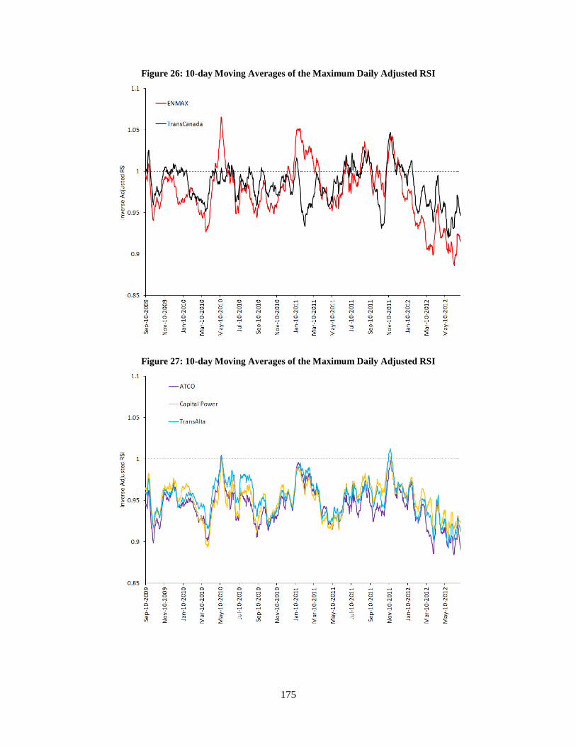
175
Figure 26: 10-day Moving Averages of the Maximum Daily Adjusted RSI
Figure 27: 10-day Moving Averages of the Maximum Daily Adjusted RSI

176
As with the residual demand analysis, the adjusted RSI metric shows that the ability of each firm
to exercise market power varied across the sample period. In addition, the Adjusted RSI analysis
highlights many of the same peaks as the residual demand estimates. For example many of the
larger firms saw peaks in their ability to exercise market power during May of 2010 and in
January-February, August and November of 2011.
It is worth noting that many of these market power peaks were the result of supply-side
constraints in the Alberta electricity market. For example, the MSA’s Q2 report of 2010 shows
that transmission constraints were a significant factor in May 2010, and the extent of these
transmission issues was significant - in some hours up to 1,000 MW of generating capacity was
constrained and unavailable to the market. In terms of unilateral market power, this event
effectively caused a meaningful fall in the availability of baseload generation, thereby shifting
the market equilibrium onto the steeper portion of the supply function. In this area of the supply
function relatively small changes in generation can have a meaningful impact on market prices.
This intuition is demonstrated by the fact that both market power measures illustrate peaks in the
market power of the larger suppliers in this period.
In a similar vein, operational issues at baseload coal units were a significant factor in explaining
the market power peaks observed in January, February, August and November of 2011. Most
notably, the Sundance 1 and 2 units were, and remain, on an extended outage because of issues
with boiler corrosion. These units account for 576 MW of coal-fired capacity. The plants went
offline in mid-December of 2010 and early in January of 2011 TransAlta issued a notice of
forced majeure to the Buyer of the Sundance A PPA. From Figures 26 and 27 it is apparent that

177
these outages significantly increased supplier market power in Alberta’s electricity market
during the first two months of 2011, when cold temperatures meant market demand was high.
6.2 The Distribution of Market Power
It is important to note that the ability of generator’s to exercise market power in Alberta is often
limited to a relatively few hours. For example, Figure 28 shows the distribution of the Residual
Demand analysis for the two largest firms across the sample period. The distribution curves
illustrate that both TransCanada and ENMAX faced a meaningful amount of competition at the
margin in the majority of hours. For example, the median of TransCanada’s semi-elasticity
measure is around $0.9 (see Table 9 for some summary statistics). This implies that in 50% of
the hours, TransCanada’s influence on the market price with 1% of its dispatched generation
(generally 15 – 20 MW) is less than $1. In 80% of the hours this Figure is less than $2.14 for
TransCanada and $1.39 for ENMAX.
The distribution curves in Figure 28 also show a distinct ‘hockey-stick’ shape. The steep slope
on the right hand side implies that in the few hours that the larger firm’s do have market power,
their ability to influence the market price with a small amount of their generation is high. For
instance, in the top 5% of hours TransCanada’s residual demand estimates imply that the firm
could have influenced the pool price by more than $30 with only 1% of its dispatched
generation, and in 1% of hours the firm’s ability to influence prices with 1% of its output was
more than $160 (see Table 9).

178
Figure 28: The distribution of the Residual Demand metric for ENMAX and TransCanada
Table 9: The distribution of the Residual Demand estimates - Summary Statistics
Percentile ATCO Capital Power ENMAX TransAlta TransCanada 5% $0.04 $0.09 $0.14 $0.03 $0.18
10% $0.05 $0.12 $0.19 $0.06 $0.28 50% $0.14 $0.32 $0.52 $0.23 $0.87 80% $0.38 $0.84 $1.39 $0.60 $2.14 95% $7.41 $11.46 $19.45 $9.56 $30.75 99% $42.80 $52.39 $97.01 $50.15 $161.19
As shown, the top few hours were an important driver in determining the a firm’s average ability
to influence market prices over the sample. To see this, Figure 29 illustrates how the mean and
median of ATCO’s market power changed over the sample period. Figure 30 shows the same
analysis for TransCanada. Both Figures highlight that the mean residual demand estimates often
peak significantly above the median, showing that these market power peaks are often driven by
the firms’ market power being relatively significant in a few hours.

179
Figure 29: The Mean and Median of the Residual Demand Analysis for ATCO during peak hours
Figure 30: The Mean and Median of the Residual Demand Analysis for TransCanada during peak hours

180
Figure 31 below shows the distribution curves for the Adjusted RSI metric. Again, the inverse
adjusted RSI is reported for ease of interpretation; an increase in the inverse adjusted RSI implies
greater structural market power. As with the Residual Demand analysis, the Adjusted RSI
approach shows that the majority of hours in the Alberta wholesale market are quite competitive.
For example, the Adjusted RSI metric is less than 1 in over 90% of hours for the two largest
firms in the market (Table 10).
Figure 31: The distribution of the Adjusted RSI measure for the 5 largest generators in Alberta
Table 10: The Percentage of hours in which generators had an Inverse Adjusted RSI above a certain level
Inverse Adj. RSI ATCO Capital Power ENMAX TransAlta TransCanada
0.95 9% 12% 26% 13% 29% 1 0.8% 1.1% 7.0% 1.4% 5.9%
1.05 0.0% 0.0% 1.0% 0.0% 0.5% 1.1 0.0% 0.0% 0.1% 0.0% 0.0%

181
Figure 32 shows how the distribution of market power, as measured by the residual demand
approach, for ENMAX and TransCanada changed across hours of the day. The Figure shows the
median, 75th and 90th percentile for each hour of the day. As one would expect, the Figure
highlights that generator market power is highest during on-peak hours when demand for
electricity it relatively high. The Residual Demand analysis again highlights that the market
power of the larger generators in Alberta tends to be concentrated in relatively few hours, and
that these few hours tend to occur during on-peak periods when demand is high. In addition, the
Figure shows that the evening ramp in market demand during the winter months is an important
factor in determining generator market power.
Figure 32: The distribution of the Residual Demand estimates across weekday hours for ENMAX and TransCanada

182
Figure 33 illustrates the same hourly analysis for TransCanada’s market power using the
Adjusted RSI measure. As with the Residual Demand analysis, the Adjusted RSI measure shows
an important difference between the peak and off-peak periods – highlighting that the larger
firms normally have very little ability to influence market outcomes when demand for electricity
is low. The Adjusted RSI analysis also highlights the evening peak in market demand which
occurs around Hour Ending 18 during winter months. In addition, comparing the median of the
Adjusted RSI with the 95th percentile illustrates a similar point to the Residual Demand measure;
the market power of the larger firms in Alberta is generally limited to a few on-peak hours.
Figure 33: The distribution of TransCanada’s Adjusted RSI across weekday hours

183
6.3 Alberta Electricity Prices, Market Fundamentals and Market Power
6.3.1 The Distribution of Electricity Prices in Alberta
The average hourly pool price for electricity in Alberta from September 1st 2009 through June
30th 2012 was $59.92/MWh. During this sample period, hourly prices ranged all the way from
the price-floor at $0/MWh to the price cap at $1,000/MWh. The distribution of hourly pool
prices across the sample period is illustrated by the red curve in Figure 34. As shown, the
distribution of pool prices is skewed significantly to the right hand-side (i.e. there are a few hours
where pool prices are well above the normal level). For example, the median value of hourly
pool prices in the sample period was $30.42, or only 50% of their mean. Indeed, for almost 90%
of the hours within the sample period hourly pool prices fell below their resulting mean.
Figure 34: The Distribution of Hourly Pool Prices over the sample period

184
To illustrate the implications of this price distribution, Figure 35 shows the contribution that each
5-percentile group made to the resulting average pool price within the sample period.64 For
example, the hours within the 80 - 85th percentile of pool prices contributed $2.46, or 4%, to the
mean pool price of $59.92. The Figure illustrates that the top 5% of hours within the sample
period contributed significantly to the resulting average. In particular, the top 5% of hours
within the sample period accounted for $27, or 45%, of the resulting average pool price. The top
10% of hours accounted for $33, or 55%, of the average pool price within the sample period.
The other way of looking at this is that 90% of hours within the sample period contributed less
than 45% to the resulting average price.
Figure 35: The Value that 5 percentile groups made to the resulting Average Pool Price
64 The value contributed to the average by each group is calculated by totalling all the pool prices that fell within
each 5 percentile group and dividing by the total number of hours in the sample period.

185
6.3.2 Pool Prices, Market Demand and the Price of Natural Gas
In a competitive market, the demand for electricity will be a principal factor in determining
market prices. As demand increases, higher cost generators will be required to generate
electricity and so prices will be higher as a result. Conversely, as demand falls, only low-cost
generators are dispatched on and so prices will tend to be lower. In addition, the prevailing costs
of generating electricity will be an important factor in determining prices when the market is
competitive. As the costs of generating power increase, suppliers will offer their electricity at a
higher price, causing market prices to increase. Conversely, as input costs decrease, generators
will lower their offer price, causing market prices to fall.
As shown by Figure 36, there is a positive relationship between the demand for electricity in the
Alberta energy market and the prevailing pool price. The scatterplot illustrated in Figure 36 also
highlights that market demand is most useful for explaining the variations in market prices below
a certain level. For example, using the exponential line-of-best-fit illustrated, market demand
alone can only explain market prices of up to ~$100 and there are a number of high-priced hours
which cannot be explained by variations in market demand. Another simple way of highlighting
this is to look at correlation coefficients. When analyzing hours in which the market price was
less than $100, the correlation coefficient between the hourly demand and the resulting Pool
Price is 0.5. In contrast, when analyzing hours in which the market price was greater than $100,
the same correlation coefficient falls to 0.16.

186
Figure 36: A scatterplot of Pool Prices against hourly demand in the Energy Merit Order
As highlighted above, in the vast majority of hours, the price for electricity in Alberta is
relatively low. In the sample period, pool prices were less than $100 for 92% of the hours. The
implication here is that, for the vast majority of hours, the market is relatively competitive and in
these hours market demand is a principal factor in determining price. However, the distribution
of prices discussed above also shows that a large amount of the value in the electricity market
price occurs in the remaining hours. In particular, hours in which pool prices were greater than
$100 account for $31, or 52%, of the average pool price across the sample period. The
scatterplot and correlation coefficients shown above imply that market demand alone is a weak
instrument for explaining the variations in price during these hours. Because these hours are
principal drivers of average prices, the overall correlation between hourly market demand and
price is also fairly weak (0.26). To see this, Figure 37 illustrates how the peak daily market
demand and the daily average price have varied across the sample period. From the Figure it is

187
apparent that while some price spikes are driven by increases in demand, the daily average prices
are often elevated when prevailing demand is relatively low.
Figure 37: Daily Average Pool Prices and Peak Energy Merit Order demand over the sample period
As discussed in section 3.3, coal and gas-fired generation currently account for 84% of Alberta’s
generation capacity. Therefore, the prevailing marginal costs of Alberta’s thermal generation
can be expected to have important implications for prices when the market is competitive. While
coal-fired capacity alone covers 44% of Alberta’s capacity, almost all of the coal units in Alberta
have “mine-to-mouth” operations, meaning that the coal to feed each plant is directly located
adjacent to the power plant. Also because of the formulation of Alberta’s coal there is little
demand for Alberta’s coal resources outside of these operations. Therefore, the marginal costs of
coal generation in Alberta are relatively stable and are predominantly determined by long-term

188
contractual agreements with the mine, labour and diesel costs, and by prevailing environmental
regulations.
In contrast, there is a deep and liquid market for natural gas in Alberta and the opportunity cost
of burning natural gas to generate electricity is quite variable. Since gas-fired generation
accounts for over 40% of Alberta’s generation capacity, the prevailing price of natural gas is an
important input-cost for Alberta’s electricity market. Therefore we should expect to see a
reasonably high level of correlation between the price of natural gas and the price of electricity in
Alberta.
Figure 38: There was relatively little correlation between Pool Prices and Gas Prices in the sample period
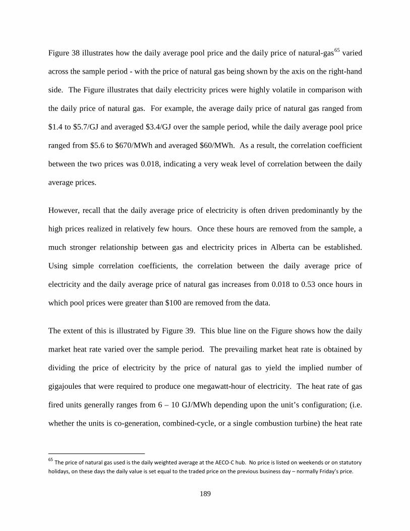
189
Figure 38 illustrates how the daily average pool price and the daily price of natural-gas65 varied
across the sample period - with the price of natural gas being shown by the axis on the right-hand
side. The Figure illustrates that daily electricity prices were highly volatile in comparison with
the daily price of natural gas. For example, the average daily price of natural gas ranged from
$1.4 to $5.7/GJ and averaged $3.4/GJ over the sample period, while the daily average pool price
ranged from $5.6 to $670/MWh and averaged $60/MWh. As a result, the correlation coefficient
between the two prices was 0.018, indicating a very weak level of correlation between the daily
average prices.
However, recall that the daily average price of electricity is often driven predominantly by the
high prices realized in relatively few hours. Once these hours are removed from the sample, a
much stronger relationship between gas and electricity prices in Alberta can be established.
Using simple correlation coefficients, the correlation between the daily average price of
electricity and the daily average price of natural gas increases from 0.018 to 0.53 once hours in
which pool prices were greater than $100 are removed from the data.
The extent of this is illustrated by Figure 39. This blue line on the Figure shows how the daily
market heat rate varied over the sample period. The prevailing market heat rate is obtained by
dividing the price of electricity by the price of natural gas to yield the implied number of
gigajoules that were required to produce one megawatt-hour of electricity. The heat rate of gas
fired units generally ranges from 6 – 10 GJ/MWh depending upon the unit’s configuration; (i.e.
whether the units is co-generation, combined-cycle, or a single combustion turbine) the heat rate
65 The price of natural gas used is the daily weighted average at the AECO-C hub. No price is listed on weekends or on statutory holidays, on these days the daily value is set equal to the traded price on the previous business day – normally Friday’s price.
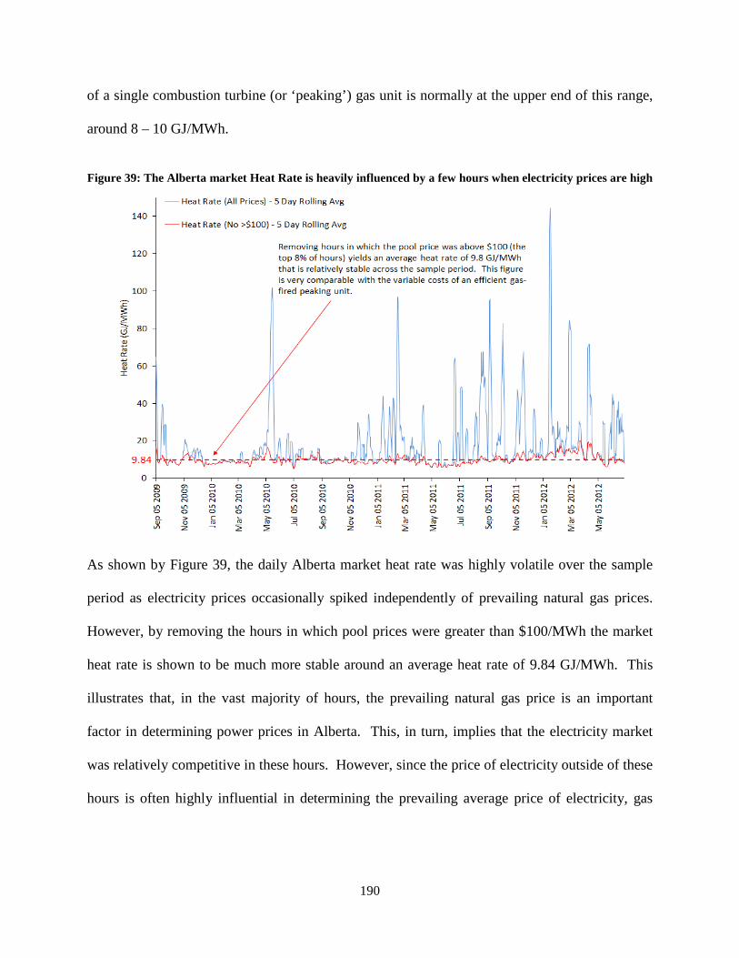
190
of a single combustion turbine (or ‘peaking’) gas unit is normally at the upper end of this range,
around 8 – 10 GJ/MWh.
Figure 39: The Alberta market Heat Rate is heavily influenced by a few hours when electricity prices are high
As shown by Figure 39, the daily Alberta market heat rate was highly volatile over the sample
period as electricity prices occasionally spiked independently of prevailing natural gas prices.
However, by removing the hours in which pool prices were greater than $100/MWh the market
heat rate is shown to be much more stable around an average heat rate of 9.84 GJ/MWh. This
illustrates that, in the vast majority of hours, the prevailing natural gas price is an important
factor in determining power prices in Alberta. This, in turn, implies that the electricity market
was relatively competitive in these hours. However, since the price of electricity outside of these
hours is often highly influential in determining the prevailing average price of electricity, gas

191
prices are shown to be substantially less relevant when analyzing Alberta electricity prices from
a broader perspective.
6.3.3 Pool Prices and Structural Market Power
Previous sections of this chapter have established that generator market power and pool prices in
the Alberta market are both variables with distributions that are significantly skewed to the right.
That is, generator market power and pool prices are both relatively low for the vast majority of
hours and occasionally these variables spike to abnormally high levels. The analysis in this
section highlights that structural market power and the resulting pool prices are variables which
are highly correlated with one another. The implication here is that the hours in which market
prices are abnormally high are also the hours in which generators in the Alberta market have the
greatest ability to influence market prices.
Figure 40 shown below illustrates the relationship between the hourly pool price and the
‘market’ inverse adjusted RSI metric. This structural market power measure illustrates the extent
to which the priced generation of the largest supplier, in that hour, is pivotal to the clearing of the
Energy Market. As shown, pool prices tend to be relatively low when the market inverse
adjusted RSI is below 0.95. As the largest generator in the Energy Market becomes increasingly
pivotal, the resulting pool prices illustrate a greater amount of variation and tend to be higher.

192
Figure 40: The relationship between the hourly Pool Price and the hourly ‘Market’ Adjusted RSI66
Figure 40 also shows that, in contrast with market demand and prevailing gas prices, the adjusted
RSI measure is reasonably correlated with higher pool price values. For example, in hours when
pool prices are greater than $100, the correlation between price and the adjusted RSI metric is
0.52. This result is corroborated by Figure 41 which plots the daily average pool price against
the daily average market inverse adjusted RSI. As shown, the daily average adjusted RSI metric
is useful in explaining variations in the daily average pool price, which in turn are often driven
by a few high priced hours.
The correlation between structural market power and the resulting pool prices is unsurprising and
does not mean that the strategic behaviour of Alberta’s largest generators is the root cause of all
high-prices. In particular, shortfalls in supply caused by unit outages, reduced wind generation,
66 The Market Adjusted RSI is the Adjusted RSI of the largest generator in that hour.

193
or transmission issues will increase both pool prices and the extent to which the larger generators
in Alberta are pivotal to the Energy Market. Therefore, analyzing the simple correlation between
these two variables cannot be used to quantify the extent to which one causes the other.
Figure 41: The Daily Average Pool Price and the Daily Average ‘Market’ Adjusted RSI
Figure 42 illustrates the relationship between the average inverse semi-elasticity of ENMAX’s
residual demand function and the monthly average pool price. Likewise, Figure 43 illustrates
how the pool price and the ability of Capital Power to influence market prices varied over the
sample period. As highlighted above, the average value of a firm’s residual demand measure is
often driven by the firm having a significant amount of market power in a few peak hours. Both
Figures illustrate a strong degree of correlation between the structural measure of market power
and the resulting pool prices. In particular, both Figures illustrate that spikes in the larger firms’
ability to influence market prices are often accompanied by price increases.

194
Again, it is important to highlight here that this correlation does not establish causation. In a
competitive market, a scarcity in supply relative to the prevailing market demand will cause
prices to increase as higher-cost units are dispatched. This increase in market tightness will also
tend to shift the market equilibrium onto a steeper portion of the supply function, where the
concentration of competing generation is often sparse. In this region of the market supply, the
residual demand functions of the larger suppliers will tend to be steeper, meaning that firms are
more able to influence the market price through offer changes. In this way, generators have the
ability to intensify the resulting price rise by pricing up their capacity when the market is tight,
and such a strategy can be highly profitable for a firm selling heavily into the resulting market
price. To analyze the extent to which firms do indeed alter their offer behaviour in response to
changing market fundamentals requires econometric analysis which controls for changes to a
firm’s marginal costs. This econometric analysis is undertaken for Alberta’s two largest
generators, ENMAX and TransCanada, in section 6.3.

195
Figure 42: ENMAX’s Monthly Average Residual Demand estimates and Monthly Average Pool Prices
Figure 43: Capital Power’s Residual Demand estimates and Pool Prices over time

196
6.3 Structural Market Power and Supplier Offer Behaviour
As highlighted in section 5.3, the incentives a firm has to exercise market power will depend
upon the firm’s overall portfolio position, or its exposure to the hourly pool price. Exercising
market power to increase price will only be a profitable strategy if the generating company is
selling into that market price. Indeed, a generating company that is actually buying from the
market may optimally exercise market power in order lower prices by running its generation
when prices are below marginal cost.
Consequently, we should expect to see that firms which are less exposed to the hourly pool price
to be less aggressive in terms of exercising market power to increase price. This section of the
thesis compares and contrasts the offer behaviour of the two largest generators in Alberta -
TransCanada and ENMAX. As shown in previous sections, these two companies are the largest
generators in Alberta and often have similar levels of structural market power across the sample
period; however, in terms of their overall portfolio these companies are considerably different.
6.3.1 ENMAX – Background and Quantitative Analysis
ENMAX Corporation is owned by the City of Calgary and consists of two subsidiaries, ENMAX
Power and ENMAX Energy Corporation. Through ENMAX Energy, ENMAX competes in the
Alberta power pool as a vertically-integrated ‘gentailer’. As well as its generation portfolio,
ENMAX Energy has a large presence in the Alberta retail electricity market. Many of these
retail sales are sold to consumers for a fixed-price. For example, ENMAX sells power to
residential consumers with its EasyMax product advertising power for a price of $89/MWh.
While this price may be based on ENMAX’s broad view of future market outcomes, the retail
price for these sales does not vary with the hourly pool price, so ENMAX is effectively buying

197
this electricity from the wholesale market at pool price, reducing the firm’s exposure.67
Therefore, ENMAX’s retail sales will cause the firm to optimally be less aggressive in exercising
market power to increase price when the firm has the ability.
It is perhaps important to emphasize that vertically integrated utilities are not uncommon in
deregulated electricity markets – for instance, electricity markets in New Zealand and Australia
both have a large degree of vertical integration. The principal rationale for vertical integration is
to reduce the risks associated with wholesale price volatility and investing in new generation
capacity. By locking in a margin above its generation costs the firm is able provide greater
certainty regarding the future profitability of its assets. This in turn reduces the risk of new
investments, which allows the firm to develop generation capacity with a lower cost of capital.
Table 11 shows the assets that ENMAX has in the Alberta wholesale market. In total the
capacity of these units sums to over 2,160 MW. However ENMAX does not have offer control
over its wind facilities and the excess energy / increased capacity its PPA units is controlled by
the PPA Owner. In its recent offer control survey the MSA estimates that ENMAX controls
1,830 MW of capacity.
67 See ENMAX (2012) Financial Report

198
Table 11: ENMAX’s Alberta generation portfolio
Asset Name Fuel Type Capacity (MW) Ownership Type
Keephills #1 Keephills #2
Coal 406 400
PPA Buyer
Battle River #1 Battle River #2 Battle River #3
Coal
149
155
389
PPA Buyer
Calgary Energy Centre (Calpine)
Natural Gas (Combined Cycle) 300 Purchased from Kelson
Canada in 2008
Crossfield #1 Crossfield #2 Crossfield #3
Natural Gas 48 48 48
Owner and operator
ENMAX Taber Wind 81 Owner and operator
Kettles Hill Wind 63 Owner and operator
McBride Lake Wind 75 50% with TransAlta
To analyze how the offer behaviour of ENMAX changes as its ability to influence the market
varies, I analyze the marginal offer price on a unit-specific basis. The marginal offer price is
defined as the highest offer price on a unit that is dispatched. A simple way to illustrate the
comparison between the marginal offer price and a firm’s market power is to plot a unit’s
marginal offer price and the firm’s Adjusted RSI as rolling averages. This simple comparison is
used to provide a gauge of the numbers involved and some overall intuition for the approach. To
determine the extent to which a firm’s structural market power alters its offer behaviour requires
thoughtful econometric analysis. This analysis is done in section 6.3.3.
Figure 44 shows how the marginal offer prices on ENMAX’s coal-fired PPA assets changed as
the firm’s ability to exercise market power varied over the sample period. The measure of
market power used here is the Inverse Adjusted RSI measure; increased values of this metric
imply a greater ability to exercise market power. As shown by the Figure, the offer behaviour on

199
ENMAX’s coal units is relatively constant and does not change as the firm’s ability to exercise
market power varies. The Keephills assets are generally dispatched around $15 while the Battle
River units are typically dispatched around $25.
Figure 44: The Max. Daily Values of ENMAX’s Market Power and the Marginal Offer Price on its coal units
Figure 45 provides the same analysis for ENMAX’s gas-fired units. The major determinant of
marginal cost for gas-fired generators is the prevailing price of natural gas. To account for
changes in the daily gas price, the Figure illustrates the marginal offered heat rate on ENMAX’s
gas units. A unit’s marginal heat rate is calculated as the unit’s marginal offer price divided by
the cost of natural gas.68 A unit’s heat rate value will vary depending on prevailing temperatures
and the unit’s current output level. An additional physical characteristic of note is that 68 The natural gas price used is the maximum daily price of natural gas traded at the AECO-C hub.

200
ENMAX’s Calpine unit has duct-firing capacity to take the unit’s generation levels above 250
MWh to a maximum of 300 MWh. This duct-firing generation is likely to be of higher cost in
comparison with the generic portion of the combined-cycle unit.
Figure 45: ENMAX’s market power and the dispatched Heat Rates on its Gas Assets
Figure 45 highlights that ENMAX’s offer behaviour on its gas plants is variable in comparison to
the offer strategies employed on its coal-fired generation. The implication here is that ENMAX
uses its coal-fired generation to meet the bulk of its retail market obligations and generally offers
these units in at marginal cost. On the other hand, ENMAX’s gas-fired assets appear to be used
either to cover for peaking levels of retail sales or to exercise market power.

201
Which of these offer strategies is optimally employed will depend upon the firm’s prevailing
corporate position, which in turn may be a function of the supply and demand fundamentals.
When ENMAX’s market power is driven by high market demand, it is likely that ENMAX’s
fixed-price retail obligations will also be high and ENMAX’s ability to influence the market may
optimally be ignored in this case, as the firm is relatively short to the pool price. In contrast,
when ENMAX’s market power is driven by a fall in the supply of competing generation,
ENMAX is more likely to be relatively long to the market price. In these cases, ENMAX may
respond by pricing up its gas units and utilizing its ability to exercise market power.
6.3.2 TransCanada – Background and Quantitative Analysis
TransCanada is a large corporation involved in natural gas and oil pipelines, natural gas storage,
as well as power generation. TransCanada’s activity in electricity markets is dominated by their
assets in Alberta, Ontario and in the Northeast of the US. Within Alberta, TransCanada is the
largest generator in the wholesale market, controlling around 2,500 MW of capacity.
As a pipelines operator, TransCanada is arguably a vertically integrated company since the
operation of its oil and gas pipelines in Alberta requires buying power from the Alberta power
pool. However, TransCanada’s pipelines operate in a regulated market where tariffs are set
based on the costs of the operations, so the electricity costs are effectively ‘flowed through’ to
pipeline users and the pipelines sector of TransCanada faces little exposure to wholesale
electricity prices.69
In comparison with ENMAX, a larger proportion of TransCanada’s generation capacity is
merchant capacity that is either sold through forward financial contracts or into the real-time
69 See Alberta MSA report on ‘Identification of Impediments to Forward Contracting’.

202
wholesale market.70 The exceptions here are TransCanada’s cogeneration facilities. Many of
TransCanada’s cogeneration assets in Alberta have been built primarily to service the demands
of an on-site host. At these facilities, TransCanada often has long-term bilateral contracts to
supply power (see Table 12).
To keep things relatively straightforward, my analysis of TransCanada will focus on the
company’s coal-fired capacity at Sundance and Sheerness and will not look at the company’s
cogeneration units. This is done so for a number of reasons. Firstly, the costs at TransCanada’s
coal-fired facilities are relatively constant because this energy is supplied to TransCanada
through long-term PPA contracts. Therefore, the operations at TransCanada’s coal facilities are
relatively straightforward and these generators are in many ways comparable with the coal-fired
assets that ENMAX controls through similar arrangements. In contrast, the operations and costs
associated the company’s cogeneration facilities are more complex and will likely change as the
operational requirements of the on-site host varies. As a result, an extreme offer price at a
cogeneration facility could be reflective of opportunity costs or operational requirements of the
on-site host.
70 TransCanada’s financial reports often provide percentage hedge levels for its Alberta power assets.

203
Table 12: TransCanada’s generation portfolio in Alberta
Asset Fuel Type Capacity (MW) Ownership Type
Sheerness #1 Sheerness #2
Coal 390
390 PPA Buyer
Sundance #1
Sundance #2 Coal
288
288 PPA Buyer
Sundance #3
Sundance #4 Coal
362
406 PPA Buyer
MacKay River Natural Gas
(Cogeneration) 185 Owner and operator – includes long-term
contracts with Suncor
Bear Creek #1 and #2
Natural Gas and Waste Heat
58 Owner and operator – includes long-term contracts with Weyerhauser 36
Carseland Natural Gas
(Cogeneration) 95
Owner and operator – includes long-term contracts with Agrium
Redwater Natural Gas
(Cogeneration) 46
Owner and operator – includes long-term contracts with Williams Energy
Cancarb Waste Heat and
Natural Gas 42
Owner and operator – a primary customer is the City of Medicine Hat
Figure 46 illustrates how the maximum daily marginal offer price on TransCanada’s Sheerness
and Sundance B (Sundance #3 and #4) assets varied as the company’s ability to exercise market
power changed over the sample period. As shown, TransCanada often increases the offer prices
on these units when the firm has the ability to exercise market power. For instance, the 10-day
moving average for both Sheerness and Sundance B peaked to over $550 in November 2011 as
these generators were dispatched at high offer prices. As shown by the Inverse Adjusted RSI,
TransCanada’s ability to exercise market power at this time was high as the metric peaked to
around 1.05. These illustrations are in contrast with the same analysis for ENMAX’s coal fired
generators, where the offer prices were shown to be relatively constant.

204
In addition, the offer behaviour of TransCanada shows a distinct change towards the end of
2010. Both Sheerness and Sundance B illustrate that TransCanada’s offer strategies were more
variable and responsive to the company’s ability to exercise market power in the latter half of the
sample period.
Figure 46: TransCanada’s market power and the dispatched offer prices on Sheerness and Sun. B
6.3.3 Econometric Analysis: Setup
To analyze the extent to which a firm alters it offer behaviour in response to changes in its ability
to exercise market power requires econometric analysis. In particular, the econometric analysis
is used to establish causation, i.e. does a change in the firm’s ability to exercise market power
cause the firm to alter its offer strategy? Fundamentally, this econometric analysis must

205
distinguish between changes in the marginal offer price that are implemented to exercise market
power from the offer changes that are the result of changes to variable costs.
At a company level, a firm’s marginal costs can vary both across generating facilities and within
generating facilities. For example, ENMAX’s marginal costs may change as the company’s
marginal generation changes from Keephills #1 at 300MW to Keephills #1 at 360MW. In
addition, the marginal costs may change as the marginal generation changes from Keephills #1 at
300MW to Crossfield #2 at 40MW. To control for cost changes adequately requires controlling
for both of these variations. To ensure that this is the case, the thesis undertakes a separate
econometric analysis for each generation facility.
For ENMAX, the facilities examined are Keephills, Battle River, Crossfield and Calpine. For
TransCanada the facilities analyzed are Sheerness, Sundance A and Sundance B. Note that there
is usually more than one generating unit at each of these facilities. For example, the Sheerness
facility consists of two generating assets. However, the operations and the cost structures of the
generators at these facilities are sufficiently uniform to prevent an individual unit-by-unit
analysis from being warranted.
For coal-fired generation, the econometric equations estimated are as follows:
𝑂𝑓𝑓𝑒𝑟 𝑃𝑟𝑖𝑐𝑒𝑈𝐻𝐷𝑀 = 𝛽0 + 𝛽1𝑀𝑃𝐽𝐻𝐷𝑀 + 𝛽2𝐹𝑟𝑜𝑚𝑈𝐻𝐷𝑀 + 𝛽3𝑇𝑜𝑈𝐻𝐷𝑀 + 𝑀𝑜𝑛𝑡ℎ + 𝐻𝑜𝑢𝑟
Where:
𝑂𝑓𝑓𝑒𝑟 𝑃𝑟𝑖𝑐𝑒𝑈𝐻𝐷𝑀 is the marginal offer price (i.e. the highest priced block that is dispatched) on
unit U in hour H on day D in month-of-the-sample M.
𝛽0 is the intercept term.

206
𝑀𝑃𝐽𝐻𝐷𝑀 is the market power metric for firm J in hour h on day D in month-of-the-sample M.
The three market power metrics used are discussed below.
𝐹𝑟𝑜𝑚𝑈𝐻𝐷𝑀 and 𝑇𝑜𝑈𝐻𝐷𝑀 show where in the units production curve the marginal block is
dispatching ‘from’ and ‘to’. For example, a unit may be dispatched a block ‘from’ 100 MWh
‘to’ 120 MWh.
𝑀𝑜𝑛𝑡ℎ are month-of-the-sample M fixed effects.
𝐻𝑜𝑢𝑟 are hourly fixed effects.
For gas-fired assets, the econometric equations are estimated as follows:
𝑂𝑓𝑓𝑒𝑟 𝑃𝑟𝑖𝑐𝑒𝑈𝐻𝐷𝑀= 𝛽0 + 𝛽1𝑀𝑃𝐽𝐻𝐷𝑀 + 𝛽2𝐹𝑟𝑜𝑚𝑈𝐻𝐷𝑀 + 𝛽3𝑇𝑜𝑈𝐻𝐷𝑀 + 𝛽4𝑇𝑒𝑚𝑝𝐻𝐷𝑀
+ 𝛽5𝑇𝑒𝑚𝑝2𝐻𝐷𝑀 + 𝐴𝐸𝐶𝑂_𝐶𝐷𝑀 + 𝑀𝑜𝑛𝑡ℎ + 𝐻𝑜𝑢𝑟
Where:
𝑂𝑓𝑓𝑒𝑟 𝑃𝑟𝑖𝑐𝑒𝑈𝐻𝐷𝑀 is the marginal offer price (i.e. the highest priced block that is dispatched)
offered by unit U in hour H on day D in month-of-the-sample M.
𝑇𝑒𝑚𝑝𝐻𝐷𝑀 is the average hourly temperature in hour H on day D in month-of-the-sample M.
𝑇𝑒𝑚𝑝2𝐻𝐷𝑀 is the average hourly temperature squared.
𝐴𝐸𝐶𝑂_𝐶𝐷𝑀 is the maximum daily price of natural gas that was traded at the AECO-C hub on
day D in month-of-the-sample M.
And the remaining terms are consistent with those defined in the previous equation.
Using this econometric approach, the major factors that affect the marginal costs of thermal
generating units are accounted for. Therefore, the 𝛽1 parameter can be interpreted as the impact

207
of an increase in the firm’s ability to exercise market power on the marginal offer price, holding
changes in marginal costs constant.
The coal facilities analyzed here are all assets which the firm has offer control of via Power
Purchase Arrangements. Under these contracts, the assets’ marginal costs are primarily a
function of a series of economic indexes and will also depend upon where the assets are in their
production curves. To control for the latter of these, the ‘from’ and ‘to’ variables are included.
The majority of the indexes used to calculate costs within the PPAs are monthly, so variations in
these indexes are captured by the month-of-the-sample fixed effects. In addition, the hourly
fixed-effects were included to allow the operational characteristics of the units to vary
systematically within days of the sample. As well, the hourly fixed effects will pick up market
effects, such as system ramping, which will vary across hours of the day and may not captured
by the market power metrics.71
For the gas-fired facilities the econometric approach is similar although a couple of changes are
made to account for additional factors. The primary input cost to control for at gas-fired
facilities is the cost of natural gas.72 To reflect this, a daily index of local natural gas prices is
included as an independent variable. Again, the ‘from’ and ‘to’ variables are included to account
for variations in marginal costs across the production curve. The monthly fixed effects are
included to account for long-term changes, such as inflation rates and labour costs, while the
hourly fixed effects are included for the same reasons outlined above. In addition, variations in
71 The market power measures are calculated using hourly-snapshot data which provides the prevailing market
fundamentals mid-way through the hour. 72 Even for units that have procured gas via a long-term fixed-price contract, the daily trading prices of natural gas
represent the opportunity cost of burning the natural gas to generate electricity.

208
the local hourly temperatures are included for gas-fired units to account for the effect that
prevailing temperatures may have on the units’ heat rate.
Market Power Measures for Econometric Analysis
From the two market power metrics developed in chapter 5, the thesis utilizes three measures of
a firm’s ability to exercise market power which are to be used in the econometric analysis. The
first two market power measures are consistent with the two measures developed in chapter 5;
the Inverse Adjusted RSI metric and the Semi-elasticity of a firm’s inverse residual demand
function. The third market power metric used here is a ‘dummy variables’ version of the Inverse
Adjusted RSI metric, which effectively splits the Inverse Adjusted RSI metric into four groups:
Table 13: The Adjusted RSI grouped analysis
Adjusted RSI Group # Lower Bound: Inverse Adjusted RSI Value (>=)
Upper Bound: Inverse Adjusted RSI Value (<)
1 - 0.85 2 0.85 0.95 3 0.95 1.00 4 1.00 -
One justification for this approach is that the effect of the Inverse adjusted RSI metric on offer
prices is often not linear. As an example of this, Figure 47 illustrates a simple scatterplot of the
Sheerness marginal offer price against the Inverse Adjusted RSI of TransCanada for the entire
sample period.

209
Figure 47: TransCanada’s market power and the marginal offer price on Sheerness
As illustrated by Figure 47, the responsiveness of TransCanada’s offer price on Sheerness to an
increase in the firm’s market power is more variable at higher values of the Inverse Adjusted
RSI. For instance, an increase in the Inverse Adjusted RSI from 0.75 to 0.85 is unlikely to have
the same impact on the firm’s offer behaviour as will a 0.1 increase from 1.00 to 1.10. In
recognition of this, some researchers (Wolak and McRae (2012) for example) abandon a refined
RSI metric in favour of a regression analysis using a simple binary variable to reflect whether or
not a firm is pivotal.
The third approach here is a hybrid of these two approaches which splits the Adjusted RSI
measures into four groups. It should be noted that other alternative model specifications, such as
taking the natural logs and including a squared term, were considered. However, the simple
approach depicted by Figure 47 above was shown to be a decent econometric model in
comparison, and also has the advantage of being easily understood. While the specific selection
$0
$100
$200
$300
$400
$500
$600
$700
$800
$900
$1,000
0.7 0.75 0.8 0.85 0.9 0.95 1 1.05 1.1 1.15
Shee
rnes
s Offe
r Pric
e
TransCanada's Inverse Adjusted RSI
Group #1 Group #2 Group #3 Group #4

210
of the group bounds is somewhat arbitrary, the selection of each group does have a considered
purpose.
Group 1 (<0.85): The first group is used throughout as a base group. Within this group, the
Inverse Adjusted RSI metric implies that the firm is very limited in its ability to exercise market
power. As shown by Figure 47 the Sheerness unit is typically dispatched at low market prices
within group #1.
Group 2 (>=0.85, <0.95): Within the second group the market participant is typically limited in
its ability to exercise market power. Occasionally, the firm may be able to drive the pool price at
higher levels of the inverse adjusted RSI within this band. This behaviour is not normal,
however, and is likely to be driven by an unusually long exposure to pool price.
Group 3 (>=0.95, <1): In the third group, the inverse adjusted RSI implies that the market
participant has a reasonable ability to influence market outcomes. Within this group the ability
of the market participant to profit from this ability will likely depend upon the firm’s net
exposure to pool price, and/or the ability of the firm’s employees to forecast the market
fundamentals two to three hours ahead of real-time.
Group 4 (>=1): Finally, in the fourth group the Inverse Adjusted RSI metric implies that the
firm’s priced generation is pivotal to the clearing of the energy market. It is reasonable to expect
that the firm will be able to forecast its ability to exercise market power in the many of these
hours. Therefore, the extent to which the participant exercises market power in these hours will
be highly depend upon the firm’s net exposure to pool price. In addition, there are likely a few
scarcity outliers in this group in which the firm may rationally conclude that offer changes are

211
not necessary to increase the market price. These scarcity events are few and far between and
thus are unlikely to affect the overall econometric results.
6.3.4 Econometric Analysis: Results
The econometric results for each of the three market power measures are illustrated by unit in
Tables 14 - 17. The reported econometric coefficients are to be interpreted as follows:
Within the Adjusted RSI Analysis the market power coefficient is to be interpreted as; a 0.1
increase in the firm’s Inverse Adjusted RSI metric causes a $ change in the marginal offer price
on the relevant unit, holding marginal costs constant. For instance, the $1.09 value on Keephills
means that as ENMAX’s inverse adjusted RSI increases by 0.1 the marginal offer price at
Keephills tends to increase by $1.09. For gas units, the Tables also report the impact of gas price
changes on the marginal offer price.
Within the Residual Demand Analysis the reported coefficients consider the impact of a $10
increase in the estimated semi-elasticity of the firm’s residual demand function on the marginal
offer price of a given unit, holding marginal cost constant.
Finally, the econometric results for the Adjusted RSI – Grouped Analysis use group #1 as the
base group. Consequently, the coefficient on each group is to be interpreted as the unit’s
marginal offer price within the given group relative to the unit’s marginal offer price within the
base group, holding marginal costs constant. For example, the arsi_3 coefficient for the
Crossfield unit is estimated as $19.70. This coefficient implies that the marginal offer price on
ENMAX’s Crossfield unit is $20 higher in group #3 than it is in group #1, holding marginal
costs constant.

212
Table 14: Econometric Results for the Adjusted RSI Analysis Adjusted RSI Analysis
ENMAX Units
Facility Coefficient Robust Standard
Error t-statistic 95% Confidence Intervals R2 N
Keephills $1.09 0.29 3.81 $0.53 $1.65 0.302 24,623
Battle River $5.94 0.27 21.80 $5.41 $6.48 0.424 24,753
Crossfield $47.48 4.32 10.99 $39.01 $55.95 0.263 6,196
CRS AECO-C $7.50 3.27 2.29 $1.08 $13.91
Calpine $21.90 1.67 13.10 $18.63 $25.18 0.264 12,889
CAL AECO-C $9.78 2.23 4.38 $5.41 $14.16
TransCanada Units
Facility Coefficient Robust Standard
Error t-statistic 95% Confidence Intervals R2 N
Sheerness $66.32 3.18 20.87 $60.09 $72.54 0.152 24,687
Sundance B $33.03 2.22 14.89 $28.68 $37.38 0.139 24,331
Sundance A $14.08 1.10 12.84 $11.93 $16.24 0.351 11,242
Table 15: Econometric Results for the Residual Demand Analysis Residual Demand Analysis
ENMAX Units
Facility Coefficient Robust Standard
Error t-statistic 95% Confidence Intervals R2 N
Keephills $0.13 0.09 1.48 -$0.04 $0.31 0.301 24,623
Battle River $0.47 0.11 4.23 $0.25 $0.69 0.396 24,753
Crossfield $0.35 0.07 5.07 $0.21 $0.48 0.255 6,196
CRS AECO-C $13.76 3.39 4.05 $7.10 $20.41
Calpine $0.34 0.06 6.03 $0.23 $0.46 0.292 12,889
CAL AECO-C $10.77 2.24 4.82 $6.38 $15.15

213
TransCanada Units
Facility Coefficient Robust Standard
Error t-statistic 95% Confidence Intervals R2 N
Sheerness $5.46 0.48 11.43 $4.53 $6.40 0.157 24,687
Sundance B $2.59 0.33 7.85 $1.94 $3.24 0.131 24,331
Sundance A $1.95 0.31 6.38 $1.35 $2.55 0.397 11,242
Table 16: The Econometric Results for the Adjusted RSI Grouped Analysis (ENMAX units) Adjusted RSI - Grouped Analysis
ENMAX Units
Facility / Group # Coefficient
Robust Standard
Error t-statistic
95% Confidence
Intervals R2 N
Keephills
arsi_2 $1.14 0.15 7.60 $0.85 $1.44
0.302 24,623 arsi_3 $1.72 0.41 4.15 $0.91 $2.53
arsi_4 $1.89 0.48 3.93 $0.95 $2.83
Battle River
arsi_2 $4.07 0.16 26.16 $3.76 $4.37
0.413 24,753 arsi_3 $6.99 0.36 19.35 $6.28 $7.70
arsi_4 $11.00 0.58 18.91 $9.86 $12.14
Crossfield
arsi_2 $12.92 2.47 5.24 $8.08 $17.75
0.245 6,196 arsi_3 $19.70 3.30 5.96 $13.23 $26.17
arsi_4 $50.82 5.77 8.80 $39.50 $62.14
AECO-C $11.39 3.45 3.30 $4.63 $18.15
Calpine
arsi_2 $1.79 1.14 1.57 -$0.45 $4.04
0.272 12,889 arsi_3 $4.28 1.64 2.61 $1.06 $7.50
arsi_4 $33.18 2.23 14.88 $28.81 $37.55
AECO-C $10.70 2.25 4.75 $6.28 $15.11

214
Table 17: The Econometric Results for the Adjusted RSI Grouped Analysis (TransCanada units) TransCanada Units
Facility / Group # Coefficient
Robust Standard
Error t-statistic
95% Confidence
Intervals R2 N
Sheerness
arsi_2 -$0.03 0.67 -0.04 -$1.34 $1.28
0.224 24,687 arsi_3 $14.01 1.51 9.27 $11.05 $16.98
arsi_4 $142.94 6.90 20.71 $129.41 $156.47
Sundance B
arsi_2 -$1.60 0.47 -3.44 -$2.51 -$0.69
0.181 24,331 arsi_3 $6.34 1.03 6.16 $4.32 $8.36
arsi_4 $81.66 5.76 14.18 $70.37 $92.95
Sundance A
arsi_2 -$2.13 0.31 -6.92 -$2.74 -$1.53
0.373 11,242 arsi_3 $6.67 0.77 8.67 $5.16 $8.17
arsi_4 $28.42 3.08 9.23 $22.38 $34.45
The econometric results obtained support the observations highlighted previously by the
quantitative analysis and intuition outlined in section 6.3.3. The pricing on ENMAX’s coal
assets is shown to be relatively unresponsive to changes in the firm’s ability to exercise unilateral
market power. The Keephills facility, in particular, is estimated to be the least responsive and
has the lowest offer price coefficient of all units within each of the market power measures. The
Battle River facility is also shown to be relatively unresponsive to market power changes,
although the units at Battle River are shown to be more responsive than the units at Keephills.
This result is intuitive since 2 of the 3 units at Battle River are substantially smaller and older
than the generators are Keephills, so it is likely that these generators have a higher variable
operating cost. A unit that has higher variable costs is cheaper to price-up / dispatch-off because
the margin that’s foregone is less, so it is unsurprising that the marginal offer price on ENMAX’s
Battle River units is more responsive than the company’s Keephills facility.

215
Both the ‘generic’ Adjusted RSI and grouped Adjusted RSI results show that ENMAX’s gas
units are far more responsive to changes in the firm’s ability to exercise market power than the
company’s coal-fired assets. This result is intuitive since gas-fired units are cheaper to start-up
and shut-down, and generally have higher variable costs than coal-fired facilities. Therefore, it is
likely optimal for ENMAX to offer its gas units at a higher price, with the risk that they are
dispatched-off, and leave its coal fired generators at low prices to ensure they remain in-merit.
In addition, the econometric results show that ENMAX’s Crossfield facility is more responsive
than the Calpine generator. For example, the marginal offer price on Crossfield is estimated to
increase by $47.48 in response to a 0.1 increase in ENMAX’s Adjusted RSI whereas the Calpine
unit’s offer price increases by $21.90. Again, this result is intuitive since Crossfield is a peaking
facility that likely has lower start-up costs and higher variable costs than the combined-cycle unit
at Calpine.
Table 18: The Econometric Results for the Cloverbar facility Capital Power’s CloverBar Peaking Unit
Adjusted RSI - Grouped Analysis
Group # Coefficient Robust Standard
Error t-statistic
95% Confidence
Intervals R2 N
arsi_2 $13.04 1.70 7.68 $9.71 $16.37
0.302 7,861 arsi_3 $48.82 3.65 13.36 $41.65 $55.98
arsi_4 $196.48 17.64 11.14 $161.91 $231.06
Adjusted RSI Analysis
Coefficient
Robust Standard
Error t-statistic
95% Confidence
Intervals R2 N
Adj. RSI $71.86 4.27 16.84 $63.49 $80.22 0.271 7,861

216
While Crossfield is shown to be relatively responsive to changes in ENMAX’s ability to exercise
market power, it is important to put these results in context. To do this, Table 18 reports the
same econometric estimates for Capital Power’s Cloverbar generating facility. The results
highlight that Capital Power’s offer behaviour on Cloverbar is more responsive to changes in the
firm’s market power in comparison to ENMAX’s Crossfield. For example, the estimated
coefficient on Cloverbar’s Adj. RSI Group #4 is almost $200, implying that the firm increases its
offer price notably when Capital Power’s ability to exercise market power is high. In
comparison, the same estimate on ENMAX’s Crossfield is $50.
This result is not surprising given that ENMAX is a vertically-integrated generator with
approximately 180 MW of wind generation. Increases in market demand and decreases in wind
generation will both increase the ability of ENMAX to exercise market power. However, both
an increase in its retail demand and a decrease in its wind generation will serve to shorten
ENMAX’s exposure to the pool price and reduce the firm’s incentives to exercise market power.
In these situations, ENMAX may optimally avoid utilizing its ability to exercise market power.
For ENMAX to profitably exercise market power requires that its exposure is relatively long
while the firm’s ability to exercise market power is also sufficiently high. For a vertically
integrated generator this combination will likely require one or both of the following:
• The firm has purchased a relatively large amount of power for a fixed price through the
forward financial markets.
• The firm’s ability to exercise market power is principally driven by outages /
transmission constraints which reduce the ability of competing generators to supply
power.

217
In contrast, ‘merchant’ generators such as TransCanada do not sell a large amount of power into
the Alberta retail market, nor does TransCanada have wind power in its generation portfolio.
Consequently, these firms are often ‘long’ to the Alberta pool price so when these firms have the
ability to increase the pool price it is often profitable for them to do so.
This intuition is most evident empirically on TransCanada’s Sheerness asset. While these two
coal-fired units are likely to have a relatively low variable cost, TransCanada often prices these
units up when the firm’s ability to influence the market price is high. For example, the
econometric results above show that the marginal offer price on Sheerness increases by some
$66 when the firm’s Adjusted RSI increases by 0.1. This result is higher than any of ENMAX’s
gas-fired units and is comparable with Capital Power’s peaking gas unit at $72. The econometric
results also shows that TransCanada’s pricing strategies on Sundance A and B were responsive
to the firm’s ability to exercise market power, although not to the same extent as Sheerness.
This ordering is somewhat surprising given that the four units at Sundance A and B are much
older than the two units at Sheerness and will likely have higher variable operating costs.
Therefore, from an economic perspective it would make more sense to increase the offer price at
Sundance A and B, and take the risk of these units being dispatched-off before the same risk is
taken with Sheerness. However these observations may be explained by other factors:
• The Sundance A units were offline for a substantial period of the sample (from December
2010 onwards). In the first half of the sample period, TransCanada appears to have been
less aggressive in pricing up its generation units in response to increases in its market
power.

218
• While TransCanada has offer control over the PPA capacity on Sundance B, the PPA was
purchased as part of a joint ownership agreement with AltaGas. The commercial
arrangements that TransCanada has with AltaGas may increase the costs of exercising
market power with these units.
6.4 The Impact of Market Events on Firm Offer Behaviour
The purpose of this section is to highlight the usefulness of the econometrics approach to analyze
the impact of market events on generators’ offer behaviour. In this section, the thesis uses the
Adjusted RSI metric to analyze the impact of the MSA’s Offer Behaviour Enforcement
Guidelines (OBEGs) on the offer behaviour of larger firms in the Alberta energy market. The
impact of the OBEGs on the Alberta market is currently the subject of a number of AUC
proceedings surrounding the risks faced by retail companies supplying the Regulated Retail
Option.73 This section begins by providing a brief background discussion of the OBEGs.
6.4.1 The OBEGs: Relevant Background
In 2010 the Alberta Market Surveillance Administrator (‘MSA’) set out to clarify the broad
meaning of its mandate so that market participants could obtain a practical understanding of
which strategies and conducts that the market monitor deemed to be inconsistent with the
relevant market regulations (notably the FEOC Regulation):
“[The Offer Behaviour Enforcement] guidelines describe the general approach of the MSA in
applying the Fair Efficient and Open Competition Regulation (FEOC Regulation) to market
participant offer behaviour in Alberta’s wholesale electricity market.” (MSA website)
73 See AUC Proceeding #2554 in particular.

219
Within the OBEGs the MSA clarified that the exercise of unilateral market power through
economic withholding is not something that, by itself, the market monitor considers to be
anticompetitive. In the final guidelines the MSA note:
“Single participant conduct aimed at capturing surplus (profits) that a market participant
has created independent of the conduct’s effect on rivals is considered competitive and
would not result in enforcement action from the MSA.
In relation to offer behaviour this means market participants are free to pursue
individually profit maximizing behaviour that does not impact on rivals’ conduct. This
would include strategies typically characterized as economic withholding.”
See MSA ‘OBEGs’ (2011)
Since its deregulation Alberta’s energy market has never been a ‘cost-based’ market and
generators have never been forced by law to offer their energy at some proxy of variable costs
(see Williams (2002) for example). However, the MSA’s consultation surrounding the OBEGs
was the first time that generators had explicit clarity that the economic withholding of generation
was not something that MSA considered to be offside of the prevailing regulations.
Section 6 of the Electric Utilities Act states that ‘[m]arket participants are to conduct themselves
in a manner that supports the fair, efficient and openly competitive operation of the market.’
Fundamentally, this is the standard against which any market participant’s conduct is to be
measured. In 2009 the FEOC Regulation was enacted, and this regulation provided some more
guidance as to participant conduct that was considered to be contrary to Section 6 of the EUA.
Section 2 of the FEOC Regulation outlines participant conduct that does not support the fair,

220
efficient and openly competitive operation of the market. Section 2 (j) of the Regulation states
that this includes “manipulating market prices, including any price index, away from a
competitive market outcome.” The FEOC Regulation does not explicitly mention economic
withholding or the exercise of unilateral market power.
Prior to the FEOC Regulation, part of the relevant legislation was ISO rule 1.10 ‘Market
Participant Behaviour Guidelines’. Within the ‘Undesirable Practices’ section of this rule, the
ISO noted:
‘When a market participant in a dominant position exploits its market power in a way that
adversely impacts upon the efficient, fair and openly competitive operation of the market,
it will be considered an abuse of dominance. Acts which constitute an abuse of
dominance include, but are not limited to, the following:
i) […]
ii) economically withholding energy by employing offering strategies so as to
adversely impact upon the efficient, fair and openly competitive operation
of the market.’
See AESO (2009c) “Comparison Between Existing and Proposed: FEOC Regulation ISO
Rules”
Prior to the OBEGs, the MSA highlighted in its 2005 report on ‘Undesirable Conduct and
Market Power’ that an abuse of market power is defined as “conduct that may be reasonably
foreseen as likely to materially undermine the fair, efficient and openly competitive operation of
the market.”

221
Overall, it is my impression that prior to MSA’s consultation in 2010 surrounding the OBEGs,
the existing legislation did not provide a clear picture as to whether the exercise of unilateral
market power was considered to be offside of the existing legislation. My interpretation is that a
blatant or systematic pattern of economic withholding might well have been labelled as an ‘abuse
of market power’. The OBEGs clarified to market participants that this was not to be the case
going forward.
In terms of timing, the MSA released the finalized OBEGs in January of 2011, having posted a
similar draft to its website in November 2010. However, the stakeholder consultation used to
formulate these final guidelines was quite extended beginning in February 2010. In terms of the
guidance surrounding unilateral market power, the MSA made it clear in these consultations that
it did not view economic withholding as anticompetitive market conduct (see “Market
Participant Offer Behaviour: Illustrative Examples”, September 2010 for example).
‘The MSA has made it clear that a strategy aimed at raising the Pool price through
economic withholding or lowering it by offering below cost, is not, by itself, going to be
challenged. Further, the MSA has stated that it will monitor behaviour of this kind but
only begin to be concerned if there is evidence that the market participant undertook
additional actions to prevent or impede competitive response, what is referred to as
abusing market power.’

222
6.4.2 The OBEGs: Econometric Analysis
To illustrate how the market power measures can be used to analyze the impact of market events
on generator offer behaviour, the thesis utilizes the econometric approach outlined in section 6.3,
using the Adjusted RSI measure and with the same independent variables being used to account
for marginal cost changes. To analyze how the offer behaviour of Alberta’s larger generators
may have changed in response to the OBEGs requires specifying when this event took effect.
For the econometric results presented below I assume that the event took place when the draft
OBEGs document was published to the MSA’s website on November 26th 2010. Therefore, from
November 26th 2010 until the end of the sample period is assumed to be post-OBEGs and prior
to this is pre-OBEGs. By splitting the sample period in two, the data can be pooled into two
separate periods and the econometrics estimates for each can be obtained.
The econometrics analysis also allows for the Wald test to be used to decipher whether the
market power coefficients in the post-OBEGs are statistically different from those observed in
the pre-OBEGs era. The results of this test are reported in the right-hand column of Table 18.
The Wald test follows the F-distribution and illustrates whether the null hypothesis, that the
market power coefficients were unchanged, can be rejected. A larger value of the resulting F-
statistic, and the associated lower probability value, implies a greater degree of certainty that the
market power coefficient changed. As shown by the results presented in Table 18, the
econometric estimates show that almost all of the assets saw a distinct change in their offer
behaviour in response to market power as a result of the OBEGs. The only exception to this is
ATCO’s Joffre asset, which has a probability of 0.12 and is subsequently rejected at the 5% or
10% significance level. For all other assets analyzed the probability is 0 to 4 decimal places
implying a strong degree of certainty that the offer behaviour of the asset altered from the pre to

223
the post-OBEGs era. In summary, the econometric analysis illustrates that generator offer
behaviour changed significantly as a result of the MSA’s OBEGs.
Table 19: Econometric Results pre and post OBEGs for various units
Generation Asset Fuel Offer Control
(Secondary)
Coefficient Pre OBEGS
(95% Confidence Intervals)
Coefficient Post OBEGs
(95% Confidence Intervals)
Estimated Change
Wald F-Test
Sheerness Coal TransCanada $20 $96
$76 213
($18 - $23) ($86 - $106) 0.0000
Sundance B Coal TransCanada
(TransAlta) $6.80 $53
$46 146
($6.07 - $7.48) ($46 - $61) 0.0000
Keephills Coal ENMAX (TransAlta)
-$0.10 $2 $2.1
17.61 (-$0.20 - $0.01) ($1 - $3) 0.0000
Battle River Coal ENMAX
(ATCO) $2.43 $8.87
$6.4 165
($2.19 - $2.67) ($7.92 - $9.82) 0.0000
Crossfield Gas ENMAX $77 $28
-$49 29
($62 - $98) ($19 - $38) 0.0000
Calpine Gas ENMAX $39 $14
-$25 32
($31 - $47) ($11 - $16) 0.0000
Gensee 3 Coal TransAlta (50%)
Capital Power (50%)
$0.69 $28 $27
100
($0.32 - $1.06) ($23 - $33) 0.0000
Poplar Creek
Gas (Cogen.) TransAlta
$7.3 $26 $18
34 ($5 - $10) ($20 - $31) 0.0000
Joffre Gas (Cogen.) ATCO
$34 $41 $7
2.37 ($28 - $40) ($35 - $47) 0.1239
Sundance C Coal Capital Power
(TransAlta) $3.49 $24
$21 60.64
($2.73 - $4.25) ($19 - $29) 0.0000
The results in Table 19 show that for a large number of assets, the impact of the OBEGs was to
increase the estimated market power coefficient. This is intuitive because, for the most part,
generating companies will be selling into the energy market and will tend to profit from higher
prices. Since the MSA’s OBEGs clarified that unilateral exercises of market power were not
offside, one would expect to see suppliers increase their use of offer strategies at higher levels of
structural market power in order to increase market prices and raise profits.

224
The econometric results for Sheerness and Sundance B imply that the OBEGs increased the
responsiveness of TransCanada to changes in the firm’s ability to exercise market power. Prior
to the OBEGs, TransCanada’s marginal offer price on Sheerness would typically increase by $20
in response to a 0.1 increase in the firm’s inverse Adjusted RSI measure. Since the draft OBEGs
were published the estimated market power coefficient is $96, implying that the OBEGs and the
associated consultation process had an important impact on TransCanada’s offer behaviour.
Figure 48 provides a quantitative illustration for how the marginal offer price on Sheerness
varied at different levels of structural market power from pre to post-OBEGs. As shown, the
offer behaviour on Sheerness changed notably at higher levels of structural market power. Prior
to the OBEGs TransCanada’s offer behaviour on Sheerness at higher levels of structural market
power was relatively reserved. For example, in hours when TransCanada’s adjusted RSI was
greater than 1.05 (meaning the firm’s priced generation was significantly pivotal) the average
marginal offer price on Sheerness in the pre-OBEGs era was little over $100. In the post-
OBEGs the same figure was close to $700. From this analysis it is apparent that the increase in
the market power coefficient on Sheerness was the result of TransCanada being more aggressive
in its attempts to increase price at higher levels of structural market power after the OBEGs.

225
Figure 48: The Average Marginal Offer Price on Sheerness at different levels of market power
As well as Sundance B and Sheerness, Table 19 also highlights a meaningful increase in the
market power coefficient on Genesee 3, Sundance C and Poplar Creek. The change in offer
behaviour on Genesee 3 is particularly striking because prior to the OBEGs the market power
coefficient was barely significant from $0, implying that the unit was consistently offered at, or
very close to, marginal cost throughout pre-OBEGs, and the structural market power of
TransAlta and Capital Power was irrelevant in determining the generator’s marginal offer price.
In the period after the draft OBEGs, the average structural market power of TransAlta and
Capital Power became significantly more apparent, with the coefficient estimated at $28. As
shown by Figure 49 it is again clear that this increase is the result of the asset being offered at
higher prices when the firms have the ability to increase market prices by doing so.

226
Figure 49: The Average Marginal Offer Price on Genesee #3 at different levels of market power
As with the econometric results detailed in section 6.3, the econometric results on ENMAX’s
units are again different to the econometric results on other assets. The market power coefficient
on both of ENMAX’s coal units increases marginally in the post-OBEGs although their resulting
coefficients remain modest and are still well below the estimates on other thermal units.
It is also interesting to see that that ENMAX’s gas units show a significant fall in their response
to the firm’s market power in the post-OBEGs period. A major difference between ENMAX and
the other large participants in the Alberta market is the firm’s fixed-price sales in the retail
market. As a result of these sales, ENMAX’s response to the OBEGs appears to have been
trying to mediate the offer behaviour of other participants when structural market power
estimates are high by running its gas units. The obvious explanation for this is that market
demand is often peaking when structural market power estimates are notably high. During these

227
times, it may well be in ENMAX’s best interest to keep market prices low, and reduce the costs
of serving its retail obligations. This will definitely be the case if the prevailing market tightness
is also driven by one of ENMAX’s coal units being offline. As shown by Figure 50 the fall in
the coefficients on ENMAX’s gas units is indeed the result of changes in the firm’s offer
behaviour at higher levels structural market power.
A related explanation is that loads in the province may have responded to the OBEGs, and the
resulting offer changes, by hedging their electricity consumption through long-term contracts
with ENMAX’s retail arm. Further fixed-price sales through it retail arm would increase the
incentives ENMAX has to keep pool prices low when its ability to influence these prices is quite
high.
Figure 50: The Average Marginal Offered Heat Rate on Crossfield at different levels of market power

228
To further confirm this intuition Table 20 below shows the estimated market power coefficients
on Capital Power’s Cloverbar gas units in three different segments of the sample period. Prior to
July 2011 Capital Power was effectively a vertically integrated generator with a large amount of
fixed-price sales through the EPCOR Regulated Retail Option (‘RRO’). As with ENMAX, the
initial response of Capital Power to the OBEGs caused a reduction in the estimated market
power coefficient on Cloverbar, with the estimate falling from $44 to $16. However, the
estimated coefficient subsequently increased significantly as these retail obligations were
transferred from Capital Power to EPCOR. This result again highlights the importance of
incentives in determining the extent to which generators respond to changes in their ability to
influence market outcomes.
Table 20: The impact of the OBEGs and the EPCOR RRO on Cloverbar’s offer behaviour
Generation Asset Fuel Offer
Control
Coefficient pre OBEGs and pre RRO
(95% CIs)
Coefficient post OBEGs but pre RRO
(95% CIs)
Coefficient post OBEGs and post RRO
(95% CIs)
Cloverbar Gas Capital Power
$44 ($34 – $54)
$16 ($13 – $19)
$122 ($105 – $140)
6.5 Broader Implications (a simple Counterfactual Analysis)
To discuss the broader implications of market power in the Alberta electricity market requires a
discussion of its impact on the pool prices observed in the market. It is possible to make use of
the regression results tabulated in the preceding sections in order to construct a ‘counterfactual’
market supply curve. This counterfactual supply curve could then be used to figure out what
pool prices might have been in the absence of market power being exercised by some of the
larger generators in the Alberta electricity market.

229
However, using the regression results discussed previously to analyze how offer behaviour may
have affected market prices presented a number of issues, which may indicate the need for future
refinements. Firstly, the market power measures used to obtain the regression results are focused
on the ability of generators to influence prices in the Alberta market. None of the market power
measures speak to profitability, or the incentives that the generators might have to increase prices
through changing their offers.
As discussed in section 5.3 of the thesis, the profitability of exercising market power will depend
upon the firm’s exposure to the prevailing market price. Since the firm’s exposure to pool prices
will change as their financial trading positions alter, it should be expected that a firm’s pricing
response to changes in its ability to exercise market power will not be constant over time.
Another important factor that can meaningfully influence the financial exposure of the larger
generators in Alberta is the Availability Incentive Payments (AIPs) schedule within the Power
Purchase Arrangements. Since the AIPs are based on 30-day rolling average pool prices, a
firm’s pool price exposure today will be affected by the availability of its PPA units over the
next 30 days. As a consequence, the exposure of the larger firms in Alberta to the market pool
prices is dynamic, and can be heavily influenced by expectations formed around PPA outages.74
The dynamic nature of a firm’s overall pool price exposure means that firms will optimally vary
how responsive their offer prices are to changing market fundamentals. In this way, it is useful
to view the regression results reported above as an average of how responsive offer prices on
74 This will be most notable in the event of a force majeure arbitration. PPA units that are offline for an extended
period will likely be subject to a claim of force majeure by the owner. At this point, the pool price exposure of the
owner may be 0 MW or -300 MW (this is just an example, the ‘target availability will depend on the size of the unit)
while the buyer’s exposure may be 0 MW or +300 MW. Neither party will know for certain until an arbitration
decision has been made, which can take upwards of 2 years.
230
particular units are to changes in a firm’s ability to influence prices. Applying these average
coefficients to specific time periods is problematic because in practice the coefficients may be
quite variable. While it is possible to run the regressions for shorter time periods, this often leads
to small sample issues. In summary, the market power measures must begin to account for
changes to a firm’s incentives in order to be useful for undertaking a counterfactual analysis.
Secondly, the regression results reported in the preceding sections use the marginal offer price as
the dependent variable. The marginal offer price is defined as the highest priced block that is
dispatched. This approach has been utilized by Wolak and McRae (2012) and Wolak (2013) to
analyze how generators respond to their ability to exercise market power in New Zealand and in
Alberta. This approach can be used to analyze how firms respond to market power changes
because a unit’s marginal offer price should remain constant in the absence of cost, production
level or operational changes. However, while changes in the marginal offer price may be
indicative of how offer prices on units are altered in accordance with changing market
fundamentals, they may not be representative of how the entire offer curve may have been
changed.75 Clearly, to determine the impact of a firm’s offer behaviour on market prices requires
considering how the entire distribution of offers is altered. In this respect, the regression analysis
could potentially be improved by using a measure of how much the offers are marked-up,
although this too raises issues such as clarifying a baseline offer price.
As a result of these issues, the prudency of using the regression results to construct an hourly
counterfactual supply curve is clearly questionable. That said, some of the overriding
75 For example, if a firm responds to an ability to exercise market power by offering half of its capacity at $25
(marginal costs) and the other half at $999.99, its marginal offer price will likely remain at $25, thus indicating no
change in offer behaviour.

231
econometric results can be used to discuss and analyze the implications of market power in the
Alberta market. As shown in section 6.3.4, the offer prices on the coal plants at Sheerness and
Sundance B are quite responsive to changes in the ability of TransCanada to exercise market
power. In addition, the market power results reported earlier highlight that in some periods
TransCanada’s ability to exercise market power is high. Therefore, it is reasonable to assume
that changing the offer prices on these units will have a material impact on the observed market
prices in some hours. In total, the four units have around 800 MW of dispatchable capacity that
can be offered into the market at a price.76
The regression results for Sheerness and Sundance B also implied that the offer prices on these
units are rarely changed when TransCanada’s Adjusted RSI index is below 0.95. Therefore, we
can make use of the marginal offer prices observed on Sheerness and Sundance B in these hours
to inform how TransCanada would offer these units in the absence of having market power. This
in turn allows us to construct a counterfactual supply curve, and analyze how much of an impact
the observed offer prices on Sheerness and Sundance B had on the resulting market prices.
In hours when TransCanada’s Adjusted RSI was below 0.95 the median marginal offer price for
Sheerness was $23.35 (this figure excludes hours when the marginal offer price is $0 because
these observations will mainly be driven by operational issues). The same figure for Sundance B
units is $23.24. However, it is not particularly abnormal to see these units dispatched at slightly
higher prices, and the 90th percentile of the marginal offer price on Sheerness in these hours is
$37, while the same figure for Sundance B is $33. Using these figures we can estimate a simple
76 The two units at Sheerness units each have a capacity of 390 MW and a minimum stable generation of 135 MW,
leaving 510 MW of dispatchable capacity that is typically available. Doing the same calculation for the two
Sundance B units yields around 260 MW of dispatchable capacity (assumes an MSG of 250 MW for each unit).

232
counterfactual supply function and begin to discuss the broader implications of market power. In
particular, for each hour in 2011 the observed supply function is altered by taking any offer
blocks on Sheerness that are priced above $37 and pricing them at $23.35. The same is also
done for Sundance B; any offers above $33 are reduced down to $23.24. The resulting
counterfactual supply curve can then be used calculated a counterfactual System Marginal Price
(SMP) for each observed SMP. This is done by assuming that the demand observed77 for each
SMP remains constant. The counterfactual SMP is then set by the highest priced block in the
counterfactual supply curve that is required to meet this demand. For each hour in 2011, the
counterfactual SMPs are used to calculate a counterfactual pool price by taking the time-
weighted average.
It is worth highlighting that this simple counterfactual analysis is subject to many of the same
criticisms outlined in section 4.8 of the literature review. In particular, the dynamic nature of the
Alberta electricity market means that changing the offer prices on Sheerness and Sundance B,
whilst holding all else constant, is unrealistic. In reality, the behaviour of other market
participants would not have been the same had Sheerness and Sundance B been offered
differently. For instance it is likely that lower offers on Sheerness and Sundance would have
caused less supply, through imports and gas-fired capacity, and potentially higher market
demand than was observed. These dynamics would imply that the counterfactual prices
calculated would be too low. On the other hand, other larger generating companies may have
responded to the high pricing on Sheerness and Sundance B by pricing-up their own units, and
had Sheerness and Sundance B been priced lower, and the market more competitive, their units
77 The number of megawatts dispatched in the Energy Market.

233
would have been offered at lower prices. This dynamic would imply that the counterfactual
prices calculated are too high.
In any case, the broader conclusions stemming from the counterfactual analysis remain
unchanged. Figures 51 and 52 illustrate the effect of lowering the offers on Sheerness and
Sundance B on the price duration curve for 2011. In 2011 the average hourly pool price
observed was $76. The counterfactual average pool price calculated was $24 less than this,
coming in at $52. Therefore, it is clear that the offer prices observed on Sheerness and Sundance
B were a significant factor in determining average pool prices in 2011.
However, as shown by the duration curves below, the pool prices observed in many hours of the
year remained largely unaffected. For instance, the 80th percentile of the observed prices is only
$6 higher than the 80th percentile of the counterfactual prices calculated. At the 90th percentile,
however, the difference between the two is $70, and by the 95th percentile the difference is $304.
It is also worth noting that at the highest percentiles, the observed and counterfactual prices
converge once again. The intuition here is that some of the highest priced hours are the result of
scarcity, and in these hours market prices would be close to the market price cap of $1,000
whether market power is being exercised or not.

234
Figure 51: Realized and Counterfactual Price Distribution Curves
Figure 52: The Realized and Counterfactual Price Distribution Curves (80th percentile and up)

235
These insights are consistent with the preceding analysis and characterization of market power in
Alberta’s electricity market. In the majority of hours the market power of the larger generating
firms is limited, and in these hours observed offer prices tend to be competitive, and pool prices
tend to be low. In the remaining hours, the larger firms do have the ability to influences prices,
and sometimes quite substantially. Therefore, in these hours, the pricing decisions that are made
by the larger firms can be an important influence on the settled prices. This relationship is
shown by Figure 53.
Figure 53: The Contribution of Adjusted RSI groups to the Average Observed and Counterfactual Prices
Figure 53 illustrates the value-added to the observed and counterfactual averages at different
levels of TransCanada’s adjusted RSI. For instance, all the hours in 2011 in which
TransCanada’s Adjusted RSI was between 0.85 and 0.9 accounted for $15 of the observed

236
average annual price. In the counterfactual calculations, these same hours show a similar level
of contribution to the average, at $13, thus indicating a small difference between the observed
and counterfactual prices in these hours, and at this level of market power. At higher levels of
structural market power the difference between the observed and counterfactual prices is more
notable. The hours in which TransCanada’s adjusted RSI is above 0.95 account for 90% of the
$24 difference in average prices. The difference in contribution is most notable for the hours in
which TransCanada’s adjusted RSI is greater than 1.0 because these hours account for 51% of
the average price difference but represent only 9% of the hours in 2011 (see Table 21).
Table 21: The Contribution of Adjusted RSI groups to the Average Prices in 2011
Adj. RSI Group
Value Add to Obs. Average
[A]
Value Add to CF Average
[B]
Difference in Value Add
[A] - [B]
Percentage of Difference
Percentage of Hours
<0.8 $0.4 $0.4 $0.0 0% 3% 0.8 - 0.85 $2.0 $2.0 $0.0 0% 12% 0.85 - 0.9 $5.6 $5.4 $0.1 1% 23% 0.9 - 0.95 $15.0 $12.6 $2.3 10% 30% 0.95 - 1 $24.2 $14.8 $9.4 39% 24%
> 1 $29.1 $17.0 $12.2 51% 9% Totals $76.2 $52.2 $24.0
These observations are important because they highlight that the successful exercise of market
power requires some level of market tightness (i.e. a shortage of competing supply relative to
market demand). In this way, the exercise of market power by the larger generators serves to
flatten out the distribution of prices at the higher end of the distribution curve. In the absence of
market power, the 85th – 99th price percentiles would undoubtedly be much lower. Under this
kind of price distribution new investment in Alberta’s energy-only would be heavily reliant on a
few hours in which the market is genuinely scarce of capacity in order to cover the fixed and

237
sunk costs. At present, these scarcity rents are limited by the $1,000 price cap and by the fact
that genuine scarcity events are few and far between.
The exercise of supplier market power will increase the profitability of generation capacity
developed in Alberta so in the long-run it should serve to incentivise new investment. In
particular, by increasing the higher end of the pool price distribution, the exercise of market
power would seem to favour the development of peaking capacity that is designed to run in the
top 15-20% of the hours. As noted by the Brattle Report (2012), this dynamic inherently means
that new entrants are reliant upon the continued exercise of market power by the incumbent
generators. However, this is a fine balance because the entry of new firms will naturally serve to
lower the market power held by the incumbent firms, thereby lowering prices. Because of this
dynamic, the economic model of Cournot predicts that new entry will only occur if the new
entrant reckons that post-entry prices will be sufficient to cover the average costs of operating.
In other words, new entry into the market should occur up until the point at which market power
becomes insufficient to warrant further entry.

238
Bibliography
Academic References
Bacalso, M. (2000), “Contractual Hazards Associated with PPAs” Department of Economics, University of Calgary
Baker, J.B. (2003), “The case for antitrust enforcement” The Journal of Economic Perspectives, 17(4), 27-50
Blumsack, S. and Lave, L.B. (2003), “Mitigating Market Power in Deregulated Electricity Markets”, mimeo, available at:
http://www.personal.psu.edu/sab51/usaee.pdf
Borenstien, S., Bushnell, J. and C. Knittel (1999), “Market Power in Electricity Markets: Beyond Concentration Measures” The Energy Journal, 20(4), 65-88
Borenstein, S. (2000), “Understanding Competitive Pricing and Market Power in Wholesale Electricity Markets” The Electricity Journal, 13(6), 49-57
Borenstein, S. (2002), “The Trouble with Electricity Markets: Understanding California's Restructuring Disaster” Journal of Economic Perspectives, 16(1), 191-211
Borenstein, S., J. Bushnell and F. Wolak (2002), “Measuring Market Inefficiencies in California's Restructured Wholesale Electricity Market” The American Economic Review, 92(5), 1376-1405
Bresnahan, T. (1987) “Competition and Collusion in the American Automobile Industry: The 1955 Price War” The Journal of Industrial Economics, 35(4), 457-482
Bresnahan, T. (1989) “Empirical studies of industries with market power” in The Handbook of Industrial Organization, Vol. II, Schmalansee, R. and Willig, R. (editors), Elsevier, Amsterdam
Church, J.R. and R. Ware (2000). Industrial Organization: A Strategic Approach. New York: McGraw-Hill Available at:
http://works.bepress.com/cgi/viewcontent.cgi?article=1022&context=jeffrey_church
Daniel, T., Doucet, J. and Plourde, A. (2007), “Electricity Industry Restructuring: The Alberta Experience”, in Electric Choices: Deregulation and the Future of Electric Power, editor A. Kleit, Rowman & Littlefield Publishers

239
Griffin, J. and S. Puller (2005), “A Primer on Electricity and the Economics of Deregulation” in Electricity Deregulation: Choices and Challenges, editors Griffin and Puller. Chicago: University of Chicago Press
Harvey, S. and W. Hogan (2001) “Identifying the Exercise of Market Power in California” The Law and Economics Consulting Group (LECG LLC), mimeo. Available at:
http://www.hks.harvard.edu/fs/whogan/Identifying%20the%20Exercise%20of%20Market%20Power%20in%20CA_122801.pdf
Harvey, S. and W. Hogan (2002) “Market Power and Market Simulations” The Law and Economics Consulting Group (LECG LLC), mimeo. Available at:
http://www.hks.harvard.edu/fs/whogan/H-H_Market_Power&Simulations_071602.pdf
Hollis, A. (2006) “The City of Calgary's Ownership of ENMAX Energy Corporation: Value at Risk” Institute for Advanced Policy Research, mimeo. Available at:
http://www.ucalgary.ca/iaprfiles/technicalpapers/iapr-tp-06010.pdf
Joskow, P. (1996), “Introducing Competition into Regulated Network Industries: from Hierarchies to Markets in Electricity” Industrial and Corporate Change, 5(2), 341-382
Joskow, P. (1997), “Restructuring, Competition and Regulatory Reform in the US Electricity Sector” The Journal of Economic Perspectives, 11(3), 119-138
Paul Joskow, P. “Comments: Remedying Undue Discrimination through Open Access Transmission Service And Standard Electricity Market Design,” mimeo. Available at:
http://regulation2point0.org/wp-content/uploads/downloads/2010/04/phpm0.pdf
Joskow, P. (2005). “The Difficult Transition to Competitive Electricity Markets in the United States” in Electricity Deregulation: Choices and Challenges, editors Griffin and Puller, University of Chicago Press
Joskow, P. and R. Schmalensee (1983) Markets for power: an analysis of electric utility deregulation. The MIT Press
Joskow, P and Kahn, E. (2002) “A quantitative analysis of pricing behavior in California's wholesale electricity market during Summer 2000” The Energy Journal 23(4), pg. 1
Nicolay, T. (2011), “Regulation by Any Other Name: Electricity Deregulation in Alberta and the Power Purchase Arrangements” Journal of Energy & Natural Resources Law, 29(1), 45-86

240
Sheffrin (2001) “Critical Actions Necessary for Effective Market Monitoring” Draft Comments Department of Market Analysis, California ISO, FERC RTO Workshop October 19. Available at:
http://www.caiso.com/docs/2001/10/19/2001101915352626702.pdf
Stoft, S (2002). Power System Economics: Designing Markets for Electricity. Wiley - IEEE Press
Thomas, E. (2003) “Market Power in the Wholesale Electricity Spot Market in Alberta” mimeo. Available at:
http://antiflux.org/~evan/papers/marketpower.pdf
Twomey, P., Green, R., Neuhoff, K. and Newbery, D. (2005), “A Review of the Monitoring of Market Power: The Possible Roles of Transmission System Operators in Monitoring for Market Power Issues in Congested Transmission Systems” Journal of Energy Literature, 11(2), 3-54
von der Fehr, N. and Harbord, D. (1993) “Spot Market Competition in the UK Electricity Industry” The Economic Journal, 103, 531-546
White (1996), “Power Struggles: Explaining Deregulatory Reforms in Electricity Markets” Brookings Papers on Economic Activity: Microeconomics, 201-250. Available at:
http://www.brookings.edu/~/media/projects/bpea/1996%20micro/1996_bpeamicro_white.pdf
Williams, R. (2002), “Williams on Electricity” Department of Economics, University of Calgary
Wipond, K. (2008), “Market Power in the Alberta Electrical Industry” Department of Economics, University of Calgary
Wolak, F. (2000), “An Empirical Analysis of the Impact of Hedge Contracts on Bidding Behaviour in a Competitive Electricity Market” International Economic Journal, 14:2, 1-39
Wolak, F. (2003), “Measuring unilateral market power in wholesale electricity markets: The california market, 1998-2000” The American Economic Review, 93:2, 425-430
Wolak, F. (2007), “Quantifying the Supply-Side Benefits from Forward Contracting in Wholesale Electricity Markets” Journal of Applied Econometrics, 22, 1179-1209
Wolak, F. (2010), “Using Restructured Electricity Supply Industries to Understand Oligopoly Industry Outcomes” Utilities Policy, 18, 227-246
Wolak, F. (2012), “Measuring the Competitiveness Benefits of a Transmission Investment Policy: The Case of the Alberta Electricity Market” mimeo. Available at:

241
http://www.stanford.edu/group/fwolak/cgi-bin/sites/default/files/files/alberta_transmission_benefits_aug_2012.pdf
Wolak, F. and S. McRae (2012) “How Do Firms Exercise Unilateral Market Power? Evidence from a Bid-Based Wholesale Electricity Market,” in Eric Brousseau and Jean-Michel Glachant (editors), Manufacturing Markets: legal, political and economic dynamics” Cambridge University Press
Wolfram, C. (1999) “Measuring Duopoly Power in the British Electricity Spot Market” The American Economic Review, 89:4, 805-826
Industry References
Alberta Electric System Operator (‘AESO’)
AESO Current and Historical Market Reports:
http://ets.aeso.ca/
AESO Long Term Outlook and Other Forecasting Publications:
http://www.aeso.ca/transmission/8638.html
AESO (2008 - ) Quarterly Long-Term Adequacy Metrics:
http://www.aeso.ca/market/22583.html
AESO (2006) “The Path to Transformation”:
http://www.aeso.ca/downloads/Path_to_Transformation_email.pdf
AESO (2009a) “Quick Hits: A Six Month Review”
http://www.aeso.ca/downloads/Quick_Hits_Review_Paper.pdf
AESO (2009b) “Currently Existing Demand Response”
http://www.aeso.ca/downloads/2009-01-27_Currently_Existing_Demand_Response.pdf
AESO (2009c) “Comparison Between Existing and Proposed: FEOC Regulation ISO Rules”
http://www.aeso.ca/downloads/Comparison_Between_Existing_and_Proposed_FEOC_Regulation_ISO_Rules.pdf

242
The Brattle Group (2011) “Evaluation of Market Fundamentals and Challenges to Long-Term System Adequacy in Alberta’s Electricity Market”:
http://www.brattle.com/_documents/UploadLibrary/Upload943.pdf
AESO (2012) Letter to Stakeholders RE Wind Pilot Project:
http://www.aeso.ca/downloads/Letter_to_Stakeholders_-_Pilot_April_26_2012.pdf
Alberta Market Surveillance Administrator
Alberta MSA (2003) “Zero Dollar Offers”:
http://albertamsa.ca/files/Zero_Offers_042903.pdf
Alberta MSA (2006) “Market Concentration Metrics”
http://albertamsa.ca/files/Market_Concentration_Metrics_110106(2).pdf
Alberta MSA (2009) “Quick Hits Review: DDS”
http://albertamsa.ca/index.php?page=notice-re-quick-hits-review-dispatch-down-service
Alberta MSA (2010 - ) Quarterly Reports
http://albertamsa.ca/index.php?page=archive
Charles Rivers Associates (2011) “Electricity Market Data Transparency”:
http://albertamsa.ca/uploads/pdf/Archive/2011/Market%20Data%20Transparency/CRA%20Report%20for%20MSA%2011-22%202011.pdf
Alberta MSA (2011) “Offer Behaviour Enforcement Guidelines”
http://albertamsa.ca/index.php?page=offer-behaviour-enforcement-guidelines
Alberta MSA (2011a) “AUC Proceeding 1553”
http://albertamsa.ca/uploads/pdf/Archive/2012/ID%201553%20-%20MSA%20Application%20November%202011.pdf
MSA (2012a) “Measuring Generator Market Power”:
http://albertamsa.ca/uploads/pdf/Archive/2012/SOTM%20Market%20Power%20103112.pdf
MSA (2012b) “State of the Market Report”:

243
http://albertamsa.ca/uploads/pdf/Archive/2012/SOTM%20Final%20Report%2020130104.pdf
MSA (2012c) “Market Share Offer Control 2012”:
http://albertamsa.ca/uploads/pdf/Archive/2012/Market%20Share%20Offer%20Control%202012.pdf
MSA (2012d) “A Comparison of the Long-Run Marginal Cost and Price of Electricity in Alberta”:
http://albertamsa.ca/uploads/pdf/Archive/2012/SOTM%20LRMC%20121012.pdf
Alberta Utilities Commission
AUC (2010) Decision 548:
http://www.auc.ab.ca/applications/decisions/Decisions/2010/2010-548.pdf
Alberta Department of Energy
London Economics (1998) “Options for Market Power Mitigation in the Alberta Power Pool”: http://www.iasa.ca/ED_documents_various/LondonEconomics.pdf
Alberta DOE (2005) “Alberta’s Electricity Policy Framework: Competitive - Reliable - Sustainable”
http://www.energy.gov.ab.ca/Electricity/pdfs/AlbertaElecFrameworkPaperJune.pdf
Current Alberta Statues and Regulations
Electric Utilities Act 2003
http://www.qp.alberta.ca/1266.cfm?page=E05P1.cfm&leg_type=Acts&isbncln=9780779759682
Fair, Efficient and Open Competition Regulation, AR 159/2009
http://www.qp.alberta.ca/1266.cfm?page=2009_159.cfm&leg_type=Regs&isbncln=9780779747719
Regulated Rate Option Regulation, AR 288/1999

244
http://www.qp.alberta.ca/1266.cfm?page=1999_288.cfm&leg_type=Regs&isbncln=9780779767878
Alberta Utilities Commission Act
http://www.qp.alberta.ca/1266.cfm?page=A37P2.cfm&leg_type=Acts&isbncln=9780779762378&display=html
Additional References
Brattle (2009): “A Comparison of PJM’s RPM with Alternative Energy and Capacity Market Designs”
http://www.brattle.com/_documents/UploadLibrary/Upload807.pdf
Brattle (2012): “ERCOT Investment Incentives and Resource Adequacy”: http://www.ercot.com/content/news/presentations/2012/Brattle%20ERCOT%20Resource%20Adequacy%20Review%20-%202012-06-01.pdf
Competition Bureau (2011) Merger Enforcement Guidelines:
http://www.competitionbureau.gc.ca/eic/site/cb-bc.nsf/vwapj/cb-meg-2011-e.pdf/$FILE/cb-meg-2011-e.pdf
Monitoring Analytics, LLC (2012) State of the Market Report for PJM
http://www.pjm.com/~/media/documents/reports/state-of-market/2012/2012-som-pjm-volume1.ashx