an analysis of shewchuk’s delaunay reﬁnement algorithm · shewchuk’s delaunay reﬁnement...

An Analysis of Shewchuk’s Delaunay

Refinement Algorithm

Hang Si

Weierstrass Institute for Applied Analysis and Stochastics (WIAS), [email protected]

Abstract. Shewchuk’s Delaunay refinement algorithm is a simple scheme to effi-ciently tetrahedralize a 3D domain. The original analysis provided guarantees ontermination and output edge lengths. However, the guarantees are weak and thetime and space complexity are not fully covered. In this paper, we present a newanalysis of this algorithm. The new analysis reduces the original 90o requirementfor the minimum input dihedral angle to arccos 1

3≈ 70.53o . The bounds on output

edge lengths and vertex degrees are improved. For a set of n input points withspread Δ (the ratio between the longest and shortest pairwise distance), we provethat the number of output points is O(n logΔ). In most cases, this bound is equiv-alent to O(n log n). This theoretically shows that the output number of tetrahedrais small.

1 Introduction

Delaunay refinement is one of the classical techniques to generate Delaunaymeshes for domains in Rd with well-shaped simplices and a small output size.It is first introduced by Chew [6] and Ruppert [18] for meshing 2D domains.

Shewchuk’s Delaunay refinement algorithm [19] (abbreviated as Shewchuk’salgorithm) is a 3D generalization of Ruppert’s [18]. This algorithm has thefeatures of being very simple and easy to implement. Practical implemen-tations [20, 22] show that it is efficient and produces tetrahedral mesheswith relatively small size compared with other size-optimal meshing algo-rithms [1, 14], see Fig. 1 for an example. Since its introduction, this algorithmhas been generalized into a number of meshing algorithms: for handling small(acute) input angles [5, 4, 17], for meshing curved domains [15, 3], and formesh adaptation [23]. However, there is no known improvement in its originalanalysis.

The original analysis of Shewchuk, which follows Ruppert’s framework [18],proved several theoretical guarantees on its termination and output edgelengths. It is observed in practice that the behaviors of this algorithm greatlyoutperforms the proved estimates. For instances, the algorithm usually ter-minates on inputs with a dihedral angle as small as 60o, which is far from

500 H. Si

Fig. 1. A three-dimensional polyhedron (left) and a boundary conforming Delaunaytetrahedral mesh generated by Shewchuk’s algorithm [19] (right).

the originally required 90o. The algorithm is able to produce a mesh whosetetrahedra having a radius-edge ratio less than

√2 (or even smaller) instead

of a value ≥ 2. The bounds on output edge lengths are obviously too large.The time and space complexity of this algorithm remain largely unsolved.

Ruppert [18] has shown that the number of output vertices of Delaunayrefinement algorithms for a domainΩ ⊂ Rd is Θ(

∫x∈Ω

1

lfs(x)ddx), where lfs(x)

is the local feature size (explained in Section 3) at a point x ∈ Ω. However,this estimate does not relate to the input. Hudson et al [10] recently proposeda variant of Shewchuk’s algorithm, the so-called Sparse Voronoi Refinement(SVR). For a set of n points in R3, SVR has runtime O(n logΔ + m) andspace usage O(m), where m is the number of output vertices and Δ is thespread of the input [8]. Note that these bounds depend on the output meshsize m which is not predictable. Recently, Miller et al [12] and Hudson etal [11] showed that under some simple assumptions on the input point sets,m linearly depends on n.

In this paper, we present a new analysis of Shewchuk’s algorithm. Ourgoal is to improve the original analysis and to gain more insight into thesimple and elegant scheme of this algorithm. Practitioners of Shewhcuk’salgorithm could be benefited from our analysis. For instances, one can avoidadding unnecessary protecting points in the problem of handling small inputangles; it may guide the choice of the order of Steiner points to reduce thetotal number of output points; and it may help in designing new Delaunayrefinement algorithms.

The rest of this paper is organized as follows. We briefly review Shewchuk’salgorithm in Section 2. In Section 3, we show that an dihedral angle boundof arccos 1

3 ≈ 70.53o is sufficient to guarantee the termination. A useful toolin our analysis is a proper sequence of added points which will be defined inSection 4. Improved bounds for output edge lengths and vertex degrees aregiven in Section 5 and Section 6, respectively. Section 7 discusses the outputmesh size. For a set of n points with spread Δ, we show that the number of

An Analysis of Shewchuk’s Delaunay Refinement Algorithm 501

output points is bounded by O(n logΔ). We end our analysis by a discussionof open issues.

2 The Algorithm

This section presents Shewchuk’s algorithm for the later analysis. Some pre-liminary definitions of the input and output objects are given first.

A piecewise linear system [24] (abbreviated as PLS) X is a collection ofpolytopes such that: (i) P ∈ X implies that all faces of P are in X , and(ii) the intersections of any two polytopes of X are again polytopes of X .The polytopes in a PLS are not necessarily convex. This definition of a PLSis generalized from Miller et al’s [13]. The dimension of a PLS is the largestdimension of its polytopes. For an example, Fig. 1 left shows a 3D PLS whichis a collection including a 3D polyhedron and all its faces. The underlyingspace |X | of X is the union of all polytopes of X , i.e., |X | = ⋃

P∈X P . Notethat |X | is a topological subspace of R3. The collection X induces a topologyon its underlying space |X |.

A tetrahedral mesh of a 3D PLS X is a finite set T of simplices, e.g.,vertices, edges, triangles, and tetrahedra, such that: (i) any two simplices ofT are either disjoint or intersect at their common face, (ii) the union of Tequals to |X |, and (iii) each polytope P ∈ X is the union of a subset of T .Fig. 1 right shows a tetrahedral mesh of a 3D PLS.

Let S be a finite set of points in Rd. A simplex σ in S is Delaunay [7] ifit has a circumscribed sphere Σ such that no other point of S lies inside Σ.Moreover, σ is Gabriel [9] if no other point of S lies inside the diametricalsphere of σ, i.e., the smallest circumscribed sphere of σ. A boundary conform-ing Delaunay mesh [24] of a 3D PLS X is a tetrahedral mesh of X such that(i) every simplex of T is Delaunay, and (ii) every simplex of T in a polytopeP ∈ X and dim(P ) < 3 is Gabriel.

The radius-edge ratio, ρ, of a tetrahedron is the ratio between the radiusof its circumscribed ball and the length of its shortest edge. The regulartetrahedron has the minimum value

√6/4 ≈ 0.612. Most of the badly shaped

tetrahedra will have a large radius-edge ratio except slivers, which are nearlydegenerate tetrahedra whose radius-edge ratio may be as small as

√2/2 ≈

0.707. Hence, strictly speaking ρ is not a shape measure. Nevertheless, it isuseful in the analysis of this algorithm.

The Algorithm: Let X be a 3D PLS. We call 1- and 2-polytopes of Xsegments and facets. Each segment and facet will be represented by a sub-complex of a mesh T of X . We call 1- and 2-simplices of that subcomplexsubsegments and subfaces to distinguish them from other simplices of T . Asubsegment (or a subface) σ is said to be encroached if it is not Gabriel inT . The algorithm is given in Fig. 2.

502 H. Si

DelaunayRefinement (X , ρ0)// X is a 3D PLS; ρ0 is a radius-edge ratio bound.1. initialize a DT D of the vertex set of X ;2. while (∃ encroached subsegment or subface)3. or (∃ τ ∈ D such that ρ(τ ) > ρ0), do4. create a new point v by rule i, i ∈ {1, 2, 3};5. update D to be the DT of vert(D) ∪ {v};6. endwhile7. T := D \ {τ | τ ∈ D and τ � |X |}8. return T ;

Fig. 2. Shewchuk’s Delaunay refinement algorithm [19]. It takes a 3D PLS X anda radius-edge ratio ρ0 as inputs, generates a boundary conforming Delaunay meshT of X such that no tetrahedra of T has radius edge ratio larger than ρ0.

After the initialization, the algorithm runs in a loop (lines 2− 6). A newpoint v (in line 4) is found by one of the three point generating rules:

R1: If a subsegment is encroached, v is its midpoint. v is an R1-vertex.R2: If a subface is encroached, v is the circumcenter of its diametric ball.

v is an R2-vertex. However, if v encroaches upon some subsegments, thenreject v, and use R1 to return a v.R3: If a tetrahedron τ has radius-edge ratio ρ(τ) > ρ0, v is its circumcen-

ter. v is an R3-vertex. However, if v encroaches upon some subsegments orsubfaces, then reject v, and use R1 or R2 to return a v.

Among these rules, R1 has the highest priority, and R3 has the lowestpriority. The priorities of the rules are important. They ensure that the newpoint v lies either inside the mesh domain or on its boundary.

3 Proof of Termination

The original analysis [19] requires that no facet angle (defined below) of theinput PLS is less than 90o. In this section, we show that this angle can bereduced.

Definitions: Let X be a 3D PLS. The local feature size [18] of a point x ∈ |X |is a function lfs : |X | → R+, such that lfs(x) is the radius of the smallestball centered at x that intersects at least two disjoint polytopes of X . Notethat lfs(x) only depends on X , it does not change when new vertices areadded in |X |. A well-known property of lfs is that it is 1-Lipschitz, i.e., forany x,y ∈ |X |, lfs(x) ≤ lfs(y)+‖x−y‖, where ‖x−y‖ denote the Euclideandistance between x and y.

For each new point v we define a parent p(v) which is a unique point re-sponsible for the addition. If v is an R1- or R2-vertex, p(v) is the encroachingpoint of v. The point p(v) may be a Delaunay vertex or a rejected circumcen-ter. If there are several encroaching points then p(v) is the one closest to v.


If two encroaching points are at the same distance to v, choose the one whichis either an input vertex or has been added earlier. If v is an R3-vertex, let τbe the tetrahedron v splits, then p(v) is one of the endpoints of the shortestedge of τ which either is an input vertex or has been added earlier. If v is aninput point, then v has no parent.

For each new point v we define the insertion radius r(v) = ‖v − p(v)‖.For an input point u ∈ X we define r(u) = ‖u − w‖, where w ∈ X is thenearest input vertex of u. Obviously, r(u) ≥ lfs(u).

An input angle of X is one of the three kinds: If two segments of X intersect,they formed an angle in |X |, it is called a segment-segment angle; if a facetintersects a non-coplanar segment, any line inside the facet and the segmentform an angle, the smallest such angle in |X | is called a segment-facet angle;if two facets intersect, they form a dihedral angle (i.e., the angle betweentheir normals) in |X |, it is called a facet-facet angle.

The following lemma is well-known. It is first proved in [19].

Lemma 1 ([19]). Let v be an added vertex, p = p(v). Let θm denote thesmallest input angle. Then:

(r1) r(v) ≥ ρ0 r(p), when v is an R3-vertex.(r2) r(v) ≥ 1√

2r(p), when v is an R1- or R2-vertex, and θm ≥ 90o.

(r3) r(v) ≥ 12 cos θ r(p), when v is an R1- or R2-vertex, and θm ≥ 45o, where

θm is either a segment-segment or a segment-facet angle;

Below we will prove a lemma for the case when θm is an acute facet-facetangle. First we will need a geometrical fact which we prove it in the followinglemma.

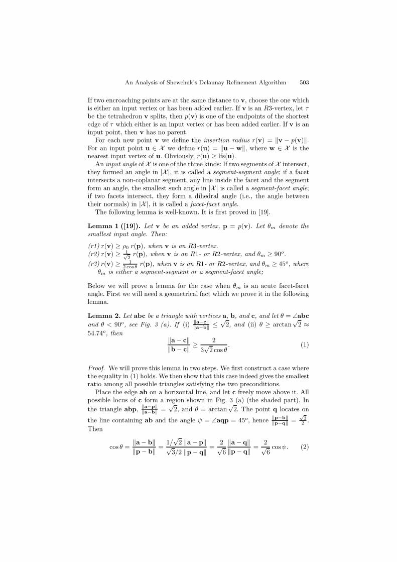
Lemma 2. Let abc be a triangle with vertices a, b, and c, and let θ = ∠abcand θ < 90o, see Fig. 3 (a). If (i) ‖a−c‖

‖a−b‖ ≤√

2, and (ii) θ ≥ arctan√

2 ≈54.74o, then

‖a− c‖‖b− c‖ ≥

23√

2 cos θ. (1)

Proof. We will prove this lemma in two steps. We first construct a case wherethe equality in (1) holds. We then show that this case indeed gives the smallestratio among all possible triangles satisfying the two preconditions.

Place the edge ab on a horizontal line, and let c freely move above it. Allpossible locus of c form a region shown in Fig. 3 (a) (the shaded part). Inthe triangle abp, ‖a−p‖

‖a−b‖ =√

2, and θ = arctan√

2. The point q locates on

the line containing ab and the angle ψ = ∠aqp = 45o, hence ‖p−b‖‖p−q‖ =

√3

2 .Then

cos θ =‖a− b‖‖p− b‖ =

1/√

2 ‖a− p‖√3/2 ‖p− q‖ =

2√6‖a− q‖‖p− q‖ =

2√6

cosψ. (2)

504 H. Si

θ ψ

a b

c

q

p

a b

c

p

θ

x c′

(a) (b)

Fig. 3. Proof of Lemma 2.

In the triangle aqp,we have the equality

‖a− p‖‖p− q‖ =

12 cosψ

,

substitute cosψ by eq. (2), and ‖p− q‖ by 2√3‖b− p‖ in above, we get

‖a− p‖‖b− p‖ =

1√6 cos θ

2√3

=2

3√

2 cos θ.

Next we show that the above ratio is the smallest one for all possiblechoices of c. First of all, if c lies inside or on the circle centered at a withradius ‖a − b‖, Pav [16] has proved that ‖a−c‖

‖b−c‖ ≥ 12 cos θ . Hence our claim

holds. In the following, we consider that c lies in the rest of the admissibleregion, see Fig. 3 (b).

For any point c in this region, we can find a point c′ which is at theintersection of the line bp and the circle C centered at a with radius ‖a−c‖,see Fig. 3 (b). It is easy to see that ‖a−c′‖

‖b−c′‖ <‖a−c‖‖b−c‖ . Now we show that

‖a−c′‖‖b−c′‖ >

‖a−p‖‖b−p‖ . Introduce an auxiliary point x at the intersection of the

circle C and the edge ap, see Fig. 3 (b), clearly, ‖x− p‖ < ‖c′ − p‖. Then

‖a− p‖‖b− p‖ =

‖a− x‖+ ‖x− p‖‖b− c′‖+ ‖c′ − p‖ ≤

‖a− c′‖‖b− c′‖ .

Since we have chosen c arbitrarily in the admissible region, so 23√

3 cos θis the

smallest ratio among all admissible choices of c.

The next lemma consider the case which is not given in Lemma 1.

Lemma 3. Let v be an added R2-vertex on facet F1, p = p(v) is an R2-vertex (not a rejected one) on facet F2. Let θ be the facet-facet angle formedby F1 and F2. Then


(r4) r(v) ≥ 13 cos θ r(p), when θ ≥ arctan

√2 ≈ 54.74o.

Proof. Let F1 v and F2 p be the two facets which intersect at a commonsegment R and form a dihedral angle θ < 90o, see Fig. 4 (a). xy is a subseg-ment of R. Let Bxy be the diametric ball of xy. Both v and p must lie outsideBxy (otherwise, xy is encroached and it must be split before we can add p orv). Let Bv denote the ball centered at v with a radius r. Bv is the diametricball of a subface on F1 encroached by p. Without loss of generality, we as-sume that v is closer to x than to y. Hence r(v) = ‖v − p‖ ≤ r ≤ ‖v − x‖,and r(p) ≤ ‖p− x‖.

Let p′ be the projection of p onto R, see Fig. 4 (b). Note that ‖v−p′‖ ≥‖v − x‖/√2, so in the triangle vp′p, ‖v−p‖

‖v−p′‖ ≤ ‖v−x‖‖v−p′‖ ≤

√2. Let θ′ be the

angle ∠vp′p. Note that θ′ ≥ θ (since θ is the dihedral angle between the twofacets). We now show that if θ ≥ arctan

√2, we can map the triangle vp′p

congruently to a triangle abc in Fig. 3 (a).

(a) (b)

(c) (d)

Fig. 4. Proof of Lemma 3.

506 H. Si

Let v = a, p′ = b, and θ′ = ∠vp′p = ∠abc. What remain is to map pto a point c in the shaded region in Fig. 3 (a). We start from a case whichv lies just on the bisector of Bxy and touch Bxy, p lies vertically on thetop of v at a distance ‖v − p‖ =

√2‖v − p′‖, see Fig. 4 (c). In this case,

θ = arctan√

2 ≈ 54.74o. Clearly vp′p is congruent to abp in Fig. 3 (a). Nowif θ > arctan

√2, since p must lie inside Bv, and v can not be inside Bxy,

hence it must be ‖v−p‖‖v−p′‖ <

√2, there exists a point c in the shaded region in

Fig. 3 (a) that can be mapped to p, and the two triangles vp′p and abc arecongruent.

So if θ ≥ arctan√

2, we can apply Lemma 2 on the triangle vp′p to get

‖v − p‖‖p′ − p‖ ≥

23√

2 cos θ′≥ 2

3√

2 cos θ. (3)

Note that ‖p − p′‖ ≥ 1√2‖p − x‖. The case when the equality holds is

shown in Fig. 4 (d), where p lies on the ball Bxy. With the help of (3), wehave ‖v − p‖

‖x− p‖ ≥1√2‖v − p‖‖p− p′‖ ≥

13 cos θ

. (4)

Remember that r(v) = ‖v − p‖, and r(p) ≤ ‖x− p‖, our claim holds bysubstituting corresponding terms in (4).

Lemma 3 allows us to prove an improved angle bound for the termination.

Theorem 1. Let X be a 3D PLS with its smallest input angle θm ≥arccos 1

3 ≈ 70.53o. Shewchuk’s algorithm terminates on X for any value ofρ0 ≥ 2.

Proof. Let lfsm = min{lfs(x) | x ∈ |X |}. We will show that no output edgeof this algorithm will have length shorter than lfsm.

Suppose for the sake of contradiction that the algorithm introduces an edgeshorter than lfsm into the mesh. Let xy be the first such edge introduced.Clearly, x and y cannot both be input vertices, nor can they lie on non-incident boundaries. Assume x was added after y. By assumption, no edgeshorter than lfsm exists before x was added, i.e., for any existing vertex q,r(q) ≥ lfsm.

Now let x be an added vertex, and p = p(x), we enumerate all the possiblecases for x and p:

• If x is an R1-vertex, and p is a rejected R3-vertex, i.e., p is the circum-center of a bad quality tetrahedron. Let g = p(p), then r(x) ≥ 1√

2r(p) ≥

ρ0√2r(g) ≥ lfsm.

• If x is an R1-vertex, and p is a rejected R2-vertex, i.e., p is the circum-center of a an encroached subface σ, and σ is encroached by a rejectedR3-vertex. Let g = p(p), and e = p(g), then r(x) ≥ 1√

2r(p) ≥ 1

2r(g) ≥ρ02 r(e) ≥ lfsm.


• If x is anR1-vertex, and p is either anR1- orR2-vertex (not rejected), i.e.,p lies on an incident segment or facet. Then r(x) ≥ 1

2 cos θmr(p) ≥ lfsm.

• If x is an R2-vertex, and p is a rejected R3-vertex. Let g = p(p), thenr(x) ≥ 1√

2r(p) ≥ ρ0√

2r(g) ≥ lfsm.

• If x is an R2-vertex, and p is an R1-vertex (not rejected) lies on anincident segment. Then r(x) ≥ 1√

2 cos θmr(p) ≥ lfsm.

• If x is an R2-vertex, and p is an R2-vertex (not rejected) lies on anincident facet. Then r(x) ≥ 1

3cosθmr(p) ≥ lfsm.

• If x is an R3-vertex, no matter what type of p has, r(x) ≥ ρ0 r(p) ≥ lfsm.

Hence r(x) ≥ lfsm in all cases, contradicting the assumption. It must bethat no edge shorter than lfsm is ever introduced, hence the algorithm willterminate.

4 Parent Sequences

Since every new vertex v has a unique parent point, we can form a sequence ofpoints by tracing the parents. In this section, we derive relations of insertionradii of a new vertex v and points in its parent sequence.

Definitions: The parent sequence of a new vertex v is a sequence of points,{vi}m+1

i=0 , such that v = v0, for i = 1, 2, ...,m, vi is an existing R3-vertex (nota rejected one), vm+1 is either an R1-, or R2-vertex, or an input vertex (i.e.,vm+1 is a boundary vertex), for i = 1, 2, ...,m, vi+1 is the parent of vi. Notethat v1 may not be the parent of v0 when v0 is an R1- or R2-vertex. Denoteg(v) = vm+1 the grandparent of v. A parent sequence of v has at least twovertices, namely v and g(v). Note that m counts the number of R3-verticesin this sequence.

Any parent sequence whose last vertex is not an input vertex can beextended to a longer sequence. We define the maximal sequence of v as asequence of parent sequences, {{vj

i }mj+1i=0 }k−1

j=0 , such that k ≥ 1, for j =0, 1, ..., k − 2, {vj

i }mj+1i=0 is a parent sequence of the vertex vj

0 (which has mj

R3-vertices), vj+10 = g(vj

0), and vk−1mk−1+1 (the last vertex) is an input vertex,

it is called the ancestor of v, denoted as a(v). An expansion of the maximalsequence of v looks like follows

k

⎧⎪⎪⎪⎪⎪⎪⎪⎪⎪⎨

⎪⎪⎪⎪⎪⎪⎪⎪⎪⎩

v = v0, v01,v

02, · · ·︸︷︷︸

m0

, v0m0+1,

v0m0+1 = v1, v1

1,v12, · · ·︸︷︷︸

m1

, v1m1+1,

· · · , · · · ,vk−2

mk−2+1 = vk−1, vk−11 ,vk−1

2 , · · ·︸︷︷︸

mk−1

, vk−1mk−1+1 = a(v).

(5)

508 H. Si

Given a geometric series with a common ratio xρ0

, let Cnx denote the sum

of its first n terms, i.e., Cnx = 1 + x

ρ0+(

xρ0

)2

+ · · · +(

xρ0

)n

= 1−(x/ρ0)n+1

1−(x/ρ0).

In particular, C0x = 1 and C∞x = 1

1−(x/ρ0) .

The following lemma derives the relations of the insertion radii of v, andg(v) for a new vertex v.

Lemma 4. Let {vi}m+1i=0 be the parent sequence of v, and let w = g(v).

(r5) If v is an R3-vertex, then r(v) ≥ ρm+10 r(w), and r(v) ≥ 1

Cm1‖v −w‖.

(r6) If v is an R2-vertex, then r(v) ≥ 1√2ρm+10 r(w), and r(v) ≥ 1

1+√

2Cm1‖v−

w‖.(r7) If v is an R1-vertex, then r(v) ≥ 1

2ρm+10 r(w), and r(v) ≥ 1

1+√

2+2Cm1‖v−

w‖.Proof. If v is an R3-vertex, for i = 0, ...,m + 1, r(vi) ≥ ρ0r(vi+1) (by(r1)). Then r(v0) ≥ ρ0r(v1) ≥ ρ2

0r(v2) ≥ · · · ≥ ρm+10 r(vm+1) =⇒ r(v) ≥

ρm+10 r(w), which is the first part of (r5). The second part of (r5) can be

proved by

‖v −w‖ ≤ ‖v0 − v1‖+ ‖v1 − v2‖+ · · ·+ ‖vm − vm+1‖= r(v0) + r(v1) + r(v2) · · ·+ r(vm)≤ (1 + 1/ρ0 + (1/ρ0)2 + · · ·+ (1/ρ0)m)r(v0)= Cm

1 r(v).

When v is an R1-vertex, v1 may not be the parent of v0. In the worstcase, there will be two rejected vertices, p and q, such that p = p(v0),

S

v2

v1

q

√2rv

√2rv

2rv

rv

2rv

e

vm

vm+1 = w

· · ·

F p

v

Fig. 5. Proof of Lemma 4. v is an R1-vertex on a segment S. p is a rejected R2-vertex on facet F (it encroaches upon the ball centered at v), and q is a rejected R3-vertex (it encroaches upon the ball centered at p). The rest vertices, v1, ...,vm+1,are in the parent sequence of v.


q = p(p), and v1 = p(q), see Fig. 5. Then by (r1), r(v0) ≥ 1√2r(p), r(p) ≥

1√2r(q), r(q) ≥ ρ0r(v1) =⇒ r(v0) ≥ 1

2ρ0r(v1). By (r5) we have r(v1) ≥ρm0 r(vm+1). Thus, r(v) ≥ 1

2ρm+10 r(w). The gives the first half of (r7). The

second half of (r7) can be proved by

‖v−w‖ ≤ ‖v0−p‖+ ‖p− q‖+ ‖q− v1‖+ ‖v1 − v2‖+ · · ·+ ‖vm − vm+1‖= r(v0) + r(p) + r(q) + r(v1) + r(v2) · · ·+ r(vm)

≤ (1 +√

2 + 2 + 2/ρ0 + 2(1/ρ0)2 + · · ·+ 2(1/ρ0)m)r(v0)

= (1 +√

2 + 2Cm1 )r(v).

Finally, the proof of (r6) is similar to the proof of (r7) and is skipped.

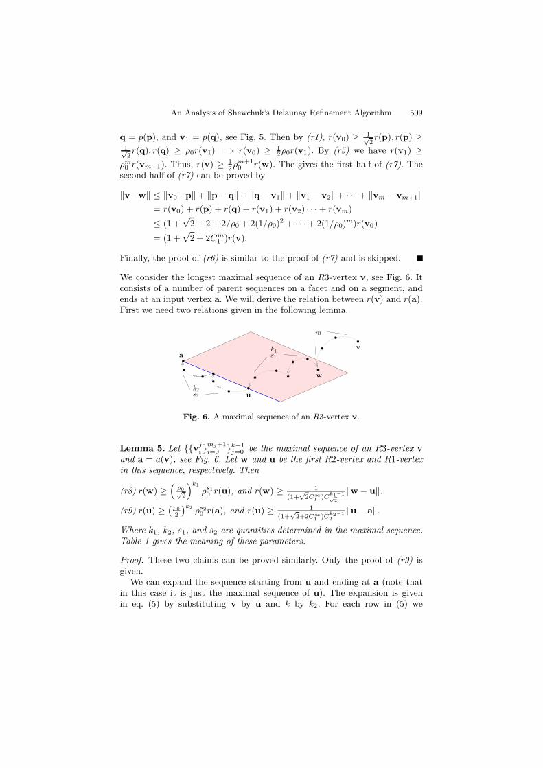
We consider the longest maximal sequence of an R3-vertex v, see Fig. 6. Itconsists of a number of parent sequences on a facet and on a segment, andends at an input vertex a. We will derive the relation between r(v) and r(a).First we need two relations given in the following lemma.

v

w

u

a

s2

s1

m

k1

k2

Fig. 6. A maximal sequence of an R3-vertex v.

Lemma 5. Let {{vji }mj+1

i=0 }k−1j=0 be the maximal sequence of an R3-vertex v

and a = a(v), see Fig. 6. Let w and u be the first R2-vertex and R1-vertexin this sequence, respectively. Then

(r8) r(w) ≥(

ρ0√2

)k1

ρs10 r(u), and r(w) ≥ 1

(1+√

2C∞1 )C

k1−1√2

‖w − u‖.(r9) r(u) ≥ (ρ0

2

)k2ρs20 r(a), and r(u) ≥ 1

(1+√

2+2C∞1 )C

k2−12

‖u− a‖.Where k1, k2, s1, and s2 are quantities determined in the maximal sequence.Table 1 gives the meaning of these parameters.

Proof. These two claims can be proved similarly. Only the proof of (r9) isgiven.

We can expand the sequence starting from u and ending at a (note thatin this case it is just the maximal sequence of u). The expansion is givenin eq. (5) by substituting v by u and k by k2. For each row in (5) we

510 H. Si

Table 1. A summary of the parameters of Lemma 5

m the number of R3-vertices between v and w m ≥ 0s1 the number of R3-vertices between w and u s1 ≥ 0s2 the number of R3-vertices between u and a s2 ≥ 0k1 the number of parent sequences between w and u k1 ≥ 1k2 the number of parent sequences between u and a k2 ≥ 1

can apply (r7): r(u0) ≥ ρ02 ρ0

m0r(u1), r(u1) ≥ ρ02 ρ0

m1r(u2), ..., r(uk2−1) ≥ρ02 ρ0

mk2−1r(a) =⇒ r(u) ≥ (ρ02

)k2ρs20 r(a). This proves the first half of (r9).

Next

‖u− a‖ ≤ ‖u0 − u1‖+ ‖u1 − u2‖+ · · ·+ ‖uk2−1 − a‖ (apply (r7))

≤ (1 +√

2 + 2Cm01 )r(u0) + (1 +

√2 + 2Cm1

1 )r(u1) + · · ·+(1 +

√2 + 2Cmk2−1

1 )r(uk2−1)

≤ (1 +√

2 + 2C∞1 )(r(u0) + r(u1) + · · ·+ r(uk2−1) (apply (r7))

≤ (1 +√

2 + 2C∞1 )(

1 +2ρ0

(1ρ0

)m0

+(

2ρ0

)2( 1ρ0

)m0+m1

+ · · ·+

(2ρ0

)k2−1( 1ρ0

)∑k2−2i=0 mi

⎞

⎠ r(u)

≤ (1 +√

2 + 2C∞1 )Ck2−12 r(u)

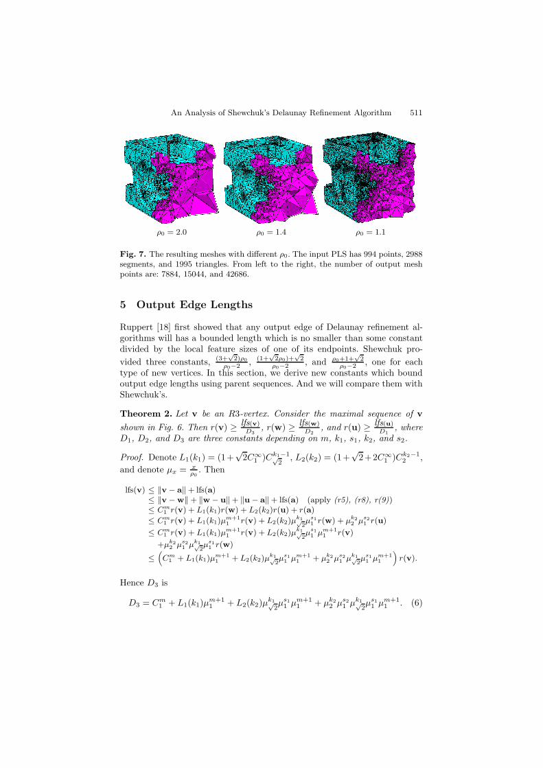
Comments on termination and mesh quality: The termination guar-antee of this algorithm requires that ρ0 ≥ 2. This is explained by the dataflow diagram in [19]. It is observed that the algorithm usually terminates ata much smaller ρ0, see Fig. 7. This fact can be explained using the maxi-mal sequence. The number m of R3-vertices in the parent sequences playsan important role which is not visible by the data flow diagram. From (r9)we see if there is at least one R3-vertex in the maximal sequence of u, thenr(u) ≥ 1

2ρ20r(a). This immediately relaxes the requirement of termination to

be ρ0 ≥√

2. Moreover, if s1 and s2 are larger (there are more R3-vertices inthe sequence), ρ0 can be much smaller.

Note that D3 is smaller if the number of R3-vertex in parent sequence (m)is large. This means vertices having a long parent sequence (which meansthey are far away from the boundary) will have longer edge lengths than thosevertices close to boundary, see Fig. 7. This also explains why the algorithmwill terminate fast.


ρ0 = 2.0 ρ0 = 1.4 ρ0 = 1.1

Fig. 7. The resulting meshes with different ρ0. The input PLS has 994 points, 2988segments, and 1995 triangles. From left to the right, the number of output meshpoints are: 7884, 15044, and 42686.

5 Output Edge Lengths

Ruppert [18] first showed that any output edge of Delaunay refinement al-gorithms will has a bounded length which is no smaller than some constantdivided by the local feature sizes of one of its endpoints. Shewchuk pro-vided three constants, (3+

√2)ρ0

ρ0−2 , (1+√

2ρ0)+√

2ρ0−2 , and ρ0+1+

√2

ρ0−2 , one for eachtype of new vertices. In this section, we derive new constants which boundoutput edge lengths using parent sequences. And we will compare them withShewchuk’s.

Theorem 2. Let v be an R3-vertex. Consider the maximal sequence of vshown in Fig. 6. Then r(v) ≥ lfs(v)

D3, r(w) ≥ lfs(w)

D2, and r(u) ≥ lfs(u)

D1, where

D1, D2, and D3 are three constants depending on m, k1, s1, k2, and s2.

Proof. Denote L1(k1) = (1+√

2C∞1 )Ck1−1√2

, L2(k2) = (1+√

2+2C∞1 )Ck2−12 ,

and denote μx = xρ0

. Then

lfs(v) ≤ ‖v − a‖+ lfs(a)≤ ‖v −w‖+ ‖w − u‖+ ‖u− a‖+ lfs(a) (apply (r5), (r8), r(9))≤ Cm

1 r(v) + L1(k1)r(w) + L2(k2)r(u) + r(a)≤ Cm

1 r(v) + L1(k1)μm+11 r(v) + L2(k2)μk1√

2μs1

1 r(w) + μk22 μs2

1 r(u)≤ Cm

1 r(v) + L1(k1)μm+11 r(v) + L2(k2)μk1√

2μs1

1 μm+11 r(v)

+μk22 μs2

1 μk1√

2μs1

1 r(w)

≤(Cm

1 + L1(k1)μm+11 + L2(k2)μk1√

2μs1

1 μm+11 + μk2

2 μs21 μ

k1√2μs1

1 μm+11

)r(v).

Hence D3 is

D3 = Cm1 + L1(k1)μm+1

1 + L2(k2)μk1√2μs1

1 μm+11 + μk2

2 μs21 μ

k1√2μs1

1 μm+11 . (6)

512 H. Si

Using the same approach, it can be shown that D1 and D2 are as follows:

D2 = L1(k1) + L2(k2)μk1√2μs1

1 + μk22 μ

s21 μ

k1√2μs1

1 , (7)

D1 = L2(k2) + μk22 μ

s21 . (8)

Since the constants D1, D2, and D3 are obtained from the longest maximalsequence of v (and for w and u as well), they are the largest ones for newvertices of the same type. In other words, they bound the edge lengths at newvertices of the same type. However, the exact values of these constants dependon their maximal sequences. Below we discuss the asymptotic behavior ofthese constants.

It can be shown that for ρ0 > 2, D1, D2, and D3 are upper bounded. Notethat increasing s1 and s2 can only make D3 smaller. The maximum of D3 isattained when m = s1 = s2 = 0, k1 = 1, and K2 →∞, which is

D3,max = C01 + (1 +

√2C∞1 )C0√

2μ1 + (1 +

√2 + 2C∞1 )C∞2 μ√2 μ1

= 1 + (1 +√

2ρ0ρ0−1 ) 1

ρ0+ (1 +

√2 + 2ρ0

ρ0−1 )√

2(ρ0−2)ρ0

The maximums of D2 and D1 are attained when k1 → ∞ and k2 → ∞,respectively,

D2,max = (1 +√

2C∞1 )C∞√2

= (1 +√

2ρ0−1 )

√2

ρ0−√

2

D1,max = (1 +√

2 + 2C∞1 )C∞2 = (1 +√

2 + 2ρ0ρ0−1 ) ρ0

ρ0−2

Compare to Shewchuk’s constants. Suppose ρ0 = 2.5. D3 is in the rangefrom 1.667 (m =∞) to 5.33 (m = s1 = s2 = 0, k1 = 1, k2 = 7). Shewchuk’sconstant (ρ0+1+

√2

ρ0−2 ) is about 9.83. D2 is in the range from 3.35 (k1 = 1) to

7.73 (k1 ≥ 25). While Shewchuk’s constant (1+√

2ρ0)+√

2ρ0−2 ) gives about 14.9.

At last, D1 is in the range from 5.75 (k2 = 1) to 28.74 (k2 ≥ 58). Shewchuk’sconstant ( (3+

√2)ρ0

ρ0−2 ) is about 22.07. Only D1,max is larger than Shewchuk’sconstant. Note that it is obtained by ignoring all R3-vertices in the maximalsequence of u which is not realistic, i.e., the estimation for (r9) is much toolarge.

6 Vertex Degrees

Talmor [25] showed that each vertex of a tetrahedral mesh with boundedradius-edge ratio only belongs to at most some fixed number of edges, andthe number only depends on the ratio. However, the constant given in [25]is miserably large1. In this section, we show a simple proof of this fact andbring the constant down to a reasonable size.1 In [25], Theorem 3.4.4, the proved constant is (2C2 +1)3, where C = CC3

2 , whichis at least (4ρ2

0)C3 , and C3 is the number of circular caps having a cone angle θdepending on ρ0 that form a cover of a unit sphere.


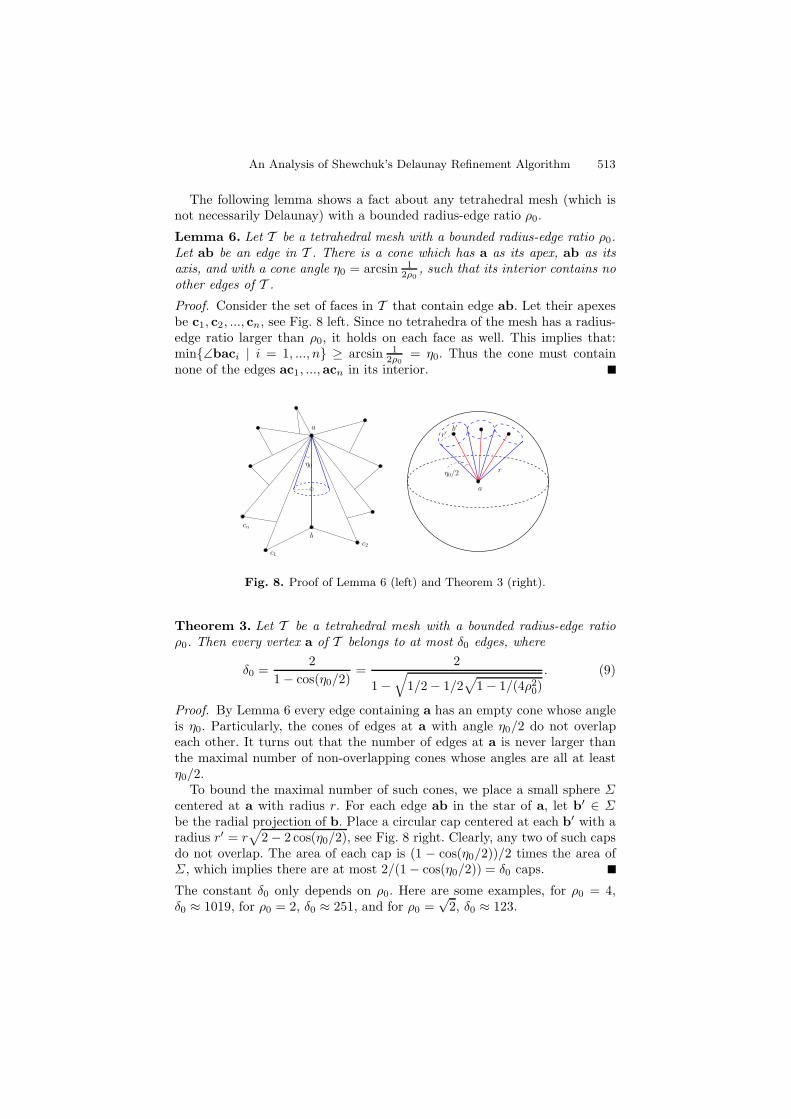
The following lemma shows a fact about any tetrahedral mesh (which isnot necessarily Delaunay) with a bounded radius-edge ratio ρ0.

Lemma 6. Let T be a tetrahedral mesh with a bounded radius-edge ratio ρ0.Let ab be an edge in T . There is a cone which has a as its apex, ab as itsaxis, and with a cone angle η0 = arcsin 1

2ρ0, such that its interior contains no

other edges of T .

Proof. Consider the set of faces in T that contain edge ab. Let their apexesbe c1, c2, ..., cn, see Fig. 8 left. Since no tetrahedra of the mesh has a radius-edge ratio larger than ρ0, it holds on each face as well. This implies that:min{∠baci | i = 1, ..., n} ≥ arcsin 1

2ρ0= η0. Thus the cone must contain

none of the edges ac1, ...,acn in its interior.

η0

a

b

c1

c2

cn

r

a

b′

η0/2

r′

Fig. 8. Proof of Lemma 6 (left) and Theorem 3 (right).

Theorem 3. Let T be a tetrahedral mesh with a bounded radius-edge ratioρ0. Then every vertex a of T belongs to at most δ0 edges, where

δ0 =2

1− cos(η0/2)=

2

1−√

1/2− 1/2√

1− 1/(4ρ20). (9)

Proof. By Lemma 6 every edge containing a has an empty cone whose angleis η0. Particularly, the cones of edges at a with angle η0/2 do not overlapeach other. It turns out that the number of edges at a is never larger thanthe maximal number of non-overlapping cones whose angles are all at leastη0/2.

To bound the maximal number of such cones, we place a small sphere Σcentered at a with radius r. For each edge ab in the star of a, let b′ ∈ Σbe the radial projection of b. Place a circular cap centered at each b′ with aradius r′ = r

√2− 2 cos(η0/2), see Fig. 8 right. Clearly, any two of such caps

do not overlap. The area of each cap is (1 − cos(η0/2))/2 times the area ofΣ, which implies there are at most 2/(1− cos(η0/2)) = δ0 caps.

The constant δ0 only depends on ρ0. Here are some examples, for ρ0 = 4,δ0 ≈ 1019, for ρ0 = 2, δ0 ≈ 251, and for ρ0 =

√2, δ0 ≈ 123.

514 H. Si

7 Output Mesh Size

In this section, we analyze the output mesh size, i.e., the number of outputvertices and tetrahedra of the Delaunay refinement algorithm.

We assume that the input is only a finite set S of points in R3. To distillthe boundary effect, we assume that S is a periodic point set [2], i.e., S ⊆[0, 1)3 is a finite set of points, and duplicated within each integer unit cube:S′ = S+Z3, where Z3 is the three-dimensional integer grid. For refining sucha point set, only the rule R3 is needed, i.e., to generate the circumcentersof bad quality tetrahedra. Let L denote the diameter of S, while s denotesthe smallest pairwise distance among input features, the ratio Δ = L/s isreferred as spread of S [8].

The following theorem shows that for a periodic point sets, the total num-ber of output points depends on the input parameters.

Theorem 4. Let S be a set of n periodic points in R3 with spread Δ. Letρ0 > 1. The output mesh of Shewchuk’s algorithm has O(n�logρ0

Δ�) vertices.

Proof. Let V denote the set of output vertices. Let | · | denote the cardinalityof a set. Hence |S| = n. We want to show that |V | = O(n�logρ0

Δ�).We first sort all new vertices produced by the algorithm into a collection of

subsets of V by the following approach: Let v be a new vertex and {vi}m+1i=0

be its parent sequence. Then it is called a rank-m vertex, i.e., there are mR3-vertices between v and g(v). Denote Vm be the set of all rank-m vertices.Let V = {V0, V1, ..., Vl−1} be the collection of all sets of rank-m vertices.Obviously, Vi ∩ Vj = ∅ for any Vi, Vj ∈ V . Hence we have

|V | = |S|+ |V0|+ |V1|+ · · ·+ |Vl−1|. (10)

Next we show that the collection V has a finite size. Note that an edgeconnecting at a rank-m vertex v has a length at least r(v). By (r5), r(v) ≥ρm+10 r(p), where p = g(v). Since here p is an input vertex, r(p) ≥ lfs(p) ≥ s.

Also note that r(v) ≤ L. Hence L ≥ r(v) ≥ ρm+10 ≥ s =⇒ ρm+1

0 ≤ L/s =⇒m+ 1 ≤ logρ0

(L/s). The largest number of subsets in V is:

l = �logρ0Δ� − 1. (11)

Next we show a key fact, that is the set V0 has the “capability” to havethe largest cardinality among all sets in V . Note it does not mean that thecardinality of V0 must be the largest in V . It means that no set in V will havea cardinality larger than the maximal possible cardinality of V0.

Let D(S) be the Delaunay tetrahedralization for S, and let V(S) be thedual Voronoi diagram of D(S). V(S) forms a space partition of the convexhull, conv(S) of S. All vertices in V(S) are candidates of rank-0 vertices to beadded by this algorithm. Let S0 be the set formed by all vertices of S and onlyrank-0 vertices (no rank-1 vertices are added yet). V(S0) is a new partition ofconv(S). A candidate for rank-1 vertex is a Voronoi vertex in V(S0) which is


the circumcenter of a bad quality tetrahedron which must have a short edgeformed by two rank-0 vertices. Obviously, the candidates for rank-1 verticesare locally restricted in V(S0) since they depend on the locations of rank-0 vertices. This shows that the space which rank-0 vertices can be addedare much larger than the space for adding rank-1 vertices. The same holdsfor vertices having higher ranks, since a new vertex is always added at the“locally sparest” location. The updated Voronoi diagram becomes sparserafter new vertices are added. Fig. 9 illustrates this fact in 2D case. Hence V0

has the capability to have the largest cardinality among other sets in V .

(a) The initial DT (b) The first added rank-1 vertex

(c) All rank-1 vertices are circled (d) All rank-2 vertices are circled

Fig. 9. Output mesh size analysis. From (a)-(d) are output meshes of a 2D Delaunayrefinement algorithm (produced by Triangle [21]) on a planar straight line graph(Lake Superior). The initial Delaunay mesh and its dual Voronoi partition are shownin (a). All Voronoi vertices are candidates of rank-0 vertices. The circled vertex in(b) is the first rank-1 vertex added by this algorithm, it is the circumcenter of theshaded triangle. For this example, the algorithm has added 326 new vertices, inwhich 313 are rank-0 vertices, 11 rank-1 vertices and 2 rank-2 vertices. (c) and (d)show the locations of rank-1 and rank-2 vertices, respectively.

It remains to find out what is the largest possible number of rank-0 vertices.Let v be an input vertex. Let e be an edge connecting at v, and e is theshortest edge of a bad quality tetrahedron t0 in a Delaunay mesh T . The worstradius-edge ratio of t0, ρ(t0) ≤ L/s = Δ. The Delaunay refinement algorithmwill remove t0 by adding its circumcenter c0. Let t1 be the tetrahedron t1 e, created by the insertion of c0. It must be ρ(t1) ≤ 1

2Δ. If ρ(t1) > ρ0,then t1 is again removed by adding its circumcenter c1. This will create anew tetrahedron t2 e, with ρ(t2) ≤ 1

4Δ. This process will repeat until atetrahedron tk e with ρ(tk) ≤ (1

2 )kΔ ≤ ρ0 is created. Hence a short edge ecould produce at most k ≤ �log2Δ� new vertices.

516 H. Si

Hence after adding at most �log2Δ� rank-0 vertices, v gets an edge whichdoes not belong to any bad quality tetrahedron. By Theorem 3, there are atmost δ0 edges connected at v, thus, after inserting at most δ0�log2Δ� vertices,all edges connecting at v do not belong to any bad quality tetrahedron. Sincethere are n input vertices, thus, the total number of rank-0 vertices are:

|V0| ≤ (δ0�log2Δ�)n. (12)

Note that δ0�log2Δ� is a constant which does not depend on n. The totalsize of V can be estimated by substituting (11) and (12) into (10),

|V | ≤ (l+ 1)(δ0�log2Δ�)n = O(n�logρ0Δ�),

The above theorem shows that for a periodic point set, the output size of theDelaunay refinement algorithm depends on n and a value logρ0

Δ. Table 2shows some tests on different values of logρ0

Δ. In this experiment, we see

Table 2. Relations between logρ0Δ and the output sizes. R10, R100, and R1k arethree PLSs. R10 is formed by two spheres, one inside the other, the outer spherehas radius r = 10 (see Fig. 10). R100 and R1k are obtained from R10 by scaling theouter sphere to the radii r = 100 and r = 1000, respectively. nin, nout, and nadd

are the number of input nodes, output nodes, and added nodes, respectively.

PLS nin ρ0 Δ logρ0Δ nout nadd

R10 772 2.0 130.10 7.022 1085 313R100 1301.08 10.350 1153 381R1k 13010.80 13.670 1208 436R10 772 1.4 130.10 14.050 1586 814R100 1301.08 20.700 1821 1049R1k 13010.80 27.345 2034 1262R10 772 1.2 130.10 26.700 2560 1788R100 1301.08 39.330 3380 2608R1k 13010.80 51.960 4081 3309

Fig. 10. Left: The PLS R10 (772 nodes, 1536 faces), formed by two spheres, oneinside the other, the outer sphere has radius r = 10, the inner one has r = 1. Right:The output Delaunay mesh (1085 nodes, 5121 tetrahedra) at ρ0 = 2.


that the value logρ0Δ approximately add a factor of O(log n) to the output

number of points.

8 Conclusions

In this paper we reanalyzed Shewchuk’s Delaunay refinement algorithm. Ournew result on the termination condition arccos 1

3 ≈ 70.53o expands the ac-ceptable class of inputs for this algorithm. The output mesh size boundO(n�logρ0

Δ�) is a theoretical guarantee that this algorithm will producesmall mesh size. Our new bounds on output edge lengths and vertex degreesbetter explain the practical behaviors of this algorithm.

However, our analysis is still far from complete. A number of interestedissues remain to be investigated. A very interested question is: Can the 70.53o

bound be reduced? Our practical experience is that a 60o bound never hurtsthe termination. In the output mesh size proof, can we show that V0 has thelargest cardinality quantitatively among other sets in V? Experiments showedthat this algorithm is able to generate a true quality mesh if it also adds thecircumcenters of slivers. In such case, what is the dihedral angle bound forall output tetrahedra?

References

1. Bern, M., Eppstein, D., Gilbert, J.R.: Provably good mesh generation. Journalof Computer and System Sciences 48(3), 384–409 (1994)

2. Cheng, S.-W., Dey, T., Edelsbrunner, H., Facello, M.A., Teng, S.-H.: Sliverexudation. J. Assoc. Comput. Mach. 47, 883–904 (2000)

3. Cheng, S.-W., Dey, T.K., Levine, J.A.: A practical Delaunay meshing algorithmfor a large class of domains. In: Proc. 16th International Meshing Roundtable,pp. 477–494 (2007)

4. Cheng, S.-W., Dey, T.K., Ramos, E.A., Ray, T.: Quality meshing for polyhe-dra with small angles. International Journal on Computational Geometry andApplications 15, 421–461 (2005)

5. Cheng, S.-W., Poon, S.-H.: Three-dimensional Delaunay mesh generation. Dis-crete and Computational Geometry 36, 419–456 (2006)

6. Chew, P.L.: Guaranteed-quality triangular meshes. Technical Report TR 89-983, Dept. of Comp. Sci., Cornell University (1989)

7. Delaunay, B.N.: Sur la sphere vide. Izvestia Akademii Nauk SSSR, OtdelenieMatematicheskikh i Estestvennykh Nauk 7, 793–800 (1934)

8. Erickson, J.: Nice point sets can have nasty Delaunay triangulations. Discreteand Computational Geometry 30(1), 109–132 (2003)

9. Gabriel, K.R., Sokal, R.R.: A new statistical approach to geographic analysis.Systematic Zoology 18(3), 259–278 (1969)

10. Hudson, B., Miller, G.L., Phillips, T.: Sparse voronoi refinement. In: Proc. 15thInternational Meshing Roundtable, pp. 339–356 (2006)

11. Hudson, B., Miller, G.L., Phillips, T., Sheehy, D.: Size complexity of volumemeshes vs. surface meshes. In: 20th Annual ACM-SIAM Symposium on DiscreteAlgorithms, pp. 1041–1047 (2009)

518 H. Si

12. Miller, G.L., Phillips, T., Sheehy, D.: Linear-size meshes. In: 20th CanadianConference on Computational Geometry (2008)

13. Miller, G.L., Talmor, D., Teng, S.-H., Walkington, N.J., Wang, H.: Controlvolume meshes using sphere packing: Generation, refinement and coarsening.In: Proc. 5th International Meshing Roundtable (1996)

14. Mitchell, S.A., Vavasis, S.A.: Quality mesh generation in higher dimensions.SIAM Journal on Computing 29, 1334–1370 (2000)

15. Oudot, S., Rineau, L., Yvinec, M.: Meshing volumes bounded by smooth sur-faces. In: Proc. 14th International Meshing Roundtable, pp. 203–220 (2005)

16. Pav, S.E.: Delaunay Refinement Algorithm. PhD thesis, Department of Mathe-matical Sciences, Carnegie Mellon University, Pittsburgh, Pennsylvania (2003)

17. Pav, S.E., Walkington, N.J.: Robust three dimensional Delaunay refinement.In: Proc. 13th International Meshing Roundtable (2004)

18. Ruppert, J.: A Delaunay refinement algorithm for quality 2-dimensional meshgeneration. Journal of Algorithms 18(3), 548–585 (1995)

19. Shewchuk, J.R.: Delaunay Refinement Mesh Generation. PhD thesis, Depart-ment of Computer Science, Carnegie Mellon University, Pittsburgh, Pennsyl-vania (1997)

20. Shewchuk, J.R.: Pyramid (2006) (Unpublished)21. Shewchuk, J.R.: Triangle (2006),

http://www.cs.cmu.edu/~quake/triangle.html

22. Si, H.: TetGen (2007), http://tetgen.berlios.de23. Si, H.: Adaptive tetrahedral mesh generation by constrained delaunay refine-

ment. International Journal for Numerical Methods in Engineering 75(7), 856–880 (2008)

24. Si, H.: Three dimensional boundary conforming Delaunay mesh generation.PhD thesis, Institute fur Mathematik, Technische Universitat Berlin (2008)

25. Talmor, D.: Well-spaced points for numerical methods. PhD thesis, Dept.of Computer Science, Carnegie Mellon University, Pittsburgh, Pennsylvania(1997)

http://www.cs.cmu.edu/~quake/triangle.html

http://tetgen.berlios.de

an analysis of shewchuk’s delaunay reﬁnement algorithm · shewchuk’s delaunay reﬁnement...

Documents