1

An Analysis of Stabilizing 3U CubeSats Using Gravity Gradient Techniques and a Low

Power Reaction Wheel

A Senior Project

presented to

the Faculty of the Aerospace Engineering Department

California Polytechnic State University, San Luis Obispo

In Partial Fulfillment

of the Requirements for the Degree

Aerospace Engineering; Bachelor of Science

by

Erich Bender

June 2011

© 2011 Erich Bender

2

An Analysis of Stabilizing 3U CubeSats Using Gravity

Gradient Techniques and a Low Power Reaction Wheel

Erich Bender

1

California Polytechnic State University – San Luis Obispo, San Luis Obispo, CA, 93401

The purpose of this paper is to determine the feasibility of gravity

gradient stabilizing a 3U CubeSat and then using a miniature reaction wheel

to further increase stability characteristics. This paper also serves as a guide

to understanding and utilizing quaternions in attitude control analysis. The

analytical results show that using 33 centimeter booms and 400 gram tip

masses, a 3U CubeSat will experience a maximum of 6 degrees of angular

displacement in yaw and pitch, and less than .5 degrees of angular

displacement in the nadir axis. A .120 kilogram miniature reaction wheel

developed by Sinclair Interplanetary was introduced into the analysis to

understand how it affected stability. Spinning at 3410 RPM and using only

160 milli-Watts of power, the wheel was placed so that it spun around the

direction of the velocity vector. The results show that a 3U CubeSat will

experience less than .05 degrees of angular displacement in all body axes over

many orbital periods.

Nomenclature Symbol

A = direction cosine element

a = reference frame vector

b = body frame vector

d = depth, m

dCM = distance from the center of mass, m

e = eigenvector

h = height, m

I = total mass moment of inertia, m4 = mass moment of inertia, m

4

J = mass moment of inertia of the reaction wheel, m4

K = Smelt parameter

l = length, m

M = gravitational moment torque, Nm

m = mass, kg

mG = mass of reaction wheel, kg

R = distance from the center of the Earth, km

r = radius, m

w = width, m

α = angular rotation around an eigenvector, degrees

ε = quaternion = quaternion change with respect to time

θ = pitch, degrees

1 Undergraduate, Aerospace Engineering Department, California Polytechnic State University – San Luis Obispo, 1

Grand Avenue, San Luis Obispo, CA, 93401

3

µ = gravitational parameter, km3/s

2

φ = roll, degrees

ψ = yaw, degrees

Ω = mean motion, m/s

ω = angular velocity, m/s = change in angular velocity with respect to time

Subscripts

x = body axis

y = body axis

z = body axis

I. Introduction

HE CubeSat project is the brainchild of California Polytechnic State University’s aerospace engineering

professor Jordi Puig-Suari and is an international collaboration of over 40 universities, high schools, and

private firms developing picosatellites containing scientific,

private, and government payloads.1 CubeSats are becoming

increasingly popular as aerospace technology companies, research

institutes (including NASA) and universities are continually

looking for alternative low cost methods with which to develop

and test new space technology for research and education that

doesn’t need the support and costs associated with that of a full

scale spacecraft. Cost to the developer is minimized by the use of

commercial-off-the-shelf products that do not require extensive

development and testing. Additionally, the launch cost to the

developer is further minimized by the small size of the total

payload, which typically is a 10cm x 10cm x 10cm cube that has a

maximum mass of 1 kilogram. The aforementioned 10cm x 10cm

x 10cm cube is known as the standard design unit or the 1U

CubeSat. It is pictured in Figure 1. There are variations on the

design of the CubeSat allowing for the picosatellites to extend

their length up to 34 cm and have a total mass of 4 kilograms –

this design is known as the 3U CubeSat.

These small picosatellites are unique

in their ability that allows them to “piggy

back” on larger scale launches and deploy

independently with no effect on the main

payload through the use of Cal Poly’s P-POD

(Poly-Picosatellite Orbital Deployer)

deployment mechanism shown in Figure 2. A

pertinent and recent example of this was with

the launch of commercial aerospace giant

SpaceX’s Dragon Capsule, which featured a

3U CubeSat called MAYFLOWER that is a

joint project between Northrop Grumman’s

NOVAWORKS division and USC’s

Department of Astronautical Engineering.

USC also provided a 1U unit called CAERUS

(the Greek word for "opportunity") to support

communications. The picosatellite CAERUS is

now orbiting around the earth about every 90

minutes at an altitude of more than 300

kilometers.4 A picture of the Dragon Capsule

T

Figure 2. P-POD deployment mechanism.3

Figure 1. A 1U CubeSat.2

4

and the attached P-PODs loaded with CubeSats is shown in Figure 3. Note the P-PODs outlined in the

boxes.

The future remains bright for the

CubeSat program as more developers are

beginning to see the practicality for picosatellite

design. In recent news, NASA has just

announced a five-year contract award to Cal

Poly to provide a broad range of P-POD services

for NASA’s own CubeSat program.5

Applications and research opportunities for new

equipment are only going to increase in the

coming years and there is a desire to take

picosatellite performance to the next level.

Unfortunately, there are some limitations to the

applications of the CubeSats, primarily anything

that would necessitate stability along any axis.

Sensors and scientific instruments that have

strict pointing requirements present a problem

for the CubeSat platform because of its lack of

axial stability. The instability issues of the

CubeSat could certainly be rectified with an active attitude determination and control system (ADCS);

however, the implications of a full ADCS on the CubeSat bus are tremendous. Such a system would require

large amounts of the minimally available on board power for utilizing small reaction wheels, as well as

power necessary for computer processing. This, in turn, would increase thermal loads and take available

power away from potential payloads.

In spite of these challenges, there is still great interest within the CubeSat community, as well as the

scientific community in expanding the capabilities of the CubeSat platform to include devices that have

strict pointing requirements. The purpose of this paper is to investigate the feasibility of stabilizing a

CubeSat, more specifically a 3U CubeSat, to rectify the aforementioned stability issue. It will be

demonstrated that implementing a combination of passive and active stabilization techniques will have

minimal impact on the other subsystems of the CubeSat. The design of the 3U CubeSat, in terms of its

shape, inherently lends itself to the applications of gravity gradient stabilization. In addition, a small reaction

wheel will be considered with the intention of providing additional stability with only minimal power

consumption. The following sections of this paper will detail the analysis required to examine this problem

followed by a direct discussion of the results. Finally, a conclusion to summarize results and remarks will be

made about the overall feasibility of stabilizing a 3U CubeSat.

II. Analysis

The first step in this analysis is to understand the shape that is being worked with. In its simplest

form, a 3U CubeSat is a rectangular prism and it will be treated as such. For the purpose of analysis, the 3U

CubeSat will be considered a homogeneous solid with its center of mass and gravity in the middle of the

prism. In addition, there are two other major components that are going to contribute to the overall mass

moments of inertia: the booms and the tip masses. One boom and tip mass is located on the top of the 3U

CubeSat, and the other boom and tip mass is located on the bottom.

Analysis of the mass moments of inertia will take place in all three coordinate axes, x, y and z. The

inertia tensor, shown in Equation 1, is a matrix of the moments of inertia, which are located on the diagonal,

and the products of inertia which fill in the other positions of the matrix.

(1)

By changing the orientation of the axes relative to the body, the moments of inertia and the

products of inertia will change in value. There is a specific and unique orientation for the x-y-z axes that

Figure 3. Dragon Capsule with P-PODs attached

(outlined in the boxes).6

5

eliminate the products of inertia and the moments of inertia maintain a constant value. The set of axes that

allows for this simplification is known as the principal axes. The inertia values located on the diagonal of the

inertia tensor are called the principal moments of inertia.7 This is demonstrated in Equation 2 below.

0

0 0

0 00 00 0 (2)

The principal axes allow for a great simplification of the otherwise computationally intensive

inertia tensor. The rest of the analysis will continue assuming that the x-y-z coordinate system of the 3U

CubeSat is aligned with the principal axes. This coordinate system is explained in greater detail at a later

point in the paper. Refer to Figure 4 for clarity.

The methodology for calculating the inertia tensor of the tip mass is shown in Equation 3. The tip

mass is assumed to be cylindrical in shape with a mass m, a height of h and a radius of r. In addition, the

principal axes will be utilized as the main coordinate system for the tip mass.

3 0 00 00 0 3

(3)

The calculation of the inertia tensor for the boom rod that holds the tip mass is shown in Equation

4. The boom rod is assumed to be a thin, slender rod with mass of m and length of l. Its coordinate system is

aligned with the principal axes and it has negligible contribution to the principal moment of inertia in the

nadir direction (z-direction) because it is a thin rod.

0 00 00 0 0 (4)

The calculation for the inertia tensor of the 3U CubeSat main body is shown in Equation 5. As

stated earlier, the body is considered to be a homogeneous solid with a mass of m, a height of h, width of w,

and a depth of d.

0 00 ! 00 0 !

(5)

In addition to the mass moments of inertia that each separate piece generates based on its own mass

and dimensions, there is also a component of inertia for each component that is not strictly located at the

center of the mass. In this case, the boom rod and the tip mass are not located at the center of mass; however,

they both have one axis going through the center of mass so the total mass moment of inertia can be easily

calculated by utilizing the parallel axis theorem, shown in Equation 6.8

"# (6)

6

I represents the total mass moment of inertia of the object. is the calculated mass moment of

inertia of the part under consideration with a mass of m. The total mass moment of inertia is a function of the

distance squared that the object is away from the center of mass, "# . Since there are two rods and two tip

masses associated with the design, the total mass moment of inertia needs to be calculated for each rod and

tip mass with respect to its position. Keep in mind that the locations of each tip mass and rod have three

components, one each in the x, y and z directions. Equation 7 shows the total mass moment of inertia tensor

for the boom rod and Equation 8 shows the total mass moment of inertia for the tip mass.

$%& $%& $%& "# (7)

'() '() '() "# (8)

The total mass moment of inertia tensor for a 3U CubeSat is the addition of the results from

Equations 5, 7 and 8 and is shown in Equation 9. The resultant tensor will be a three by three matrix with the

principal moments of inertia along the diagonal.

*+ ,%& $%&- $%&. '()- '(). (9)

While maintaining the principal axes, and with the principal moments of inertia calculated in

Equation 9, the inherent stability of the 3U CubeSat can be analyzed by non-dimensionalizing the principal

moments of inertia. This is done by setting up a constant of proportionality that is a function of each

principal moment of inertia. The constants of proportionality can then be plotted on a stability chart to

understand the natural stability characteristics of the shape under analysis. Equations 10, 11 and 12 are the

three constants of proportionality, known as Smelt parameters, for the analysis where is the principal

moment of inertia located in the upper left diagonal of the inertia tensor, is the middle diagonal and is

the lower right diagonal.

/ 0120304 (10)

/ 0320401 (11)

/* 5-25.65-5. (12)

With the principal inertias and the stability characteristics accounted for, the analysis will now

move towards describing and defining the attitude of the CubeSat in space. The attitude of a three

dimensional body is most conveniently defined with a set of axes fixed to the body. This set of axes is

generally a set of three orthogonal coordinates, or a dextral set, and is typically referred to as the body

coordinate frame. The attitude of a body is thought of as a coordinate transformation that transforms a

defined set of reference coordinates into the body coordinates of the spacecraft.9 This portion of the analysis

will begin by establishing the direction cosine matrix in Equation 13. The central matrix, which will be

referred to as the A matrix, is comprised of the three components of the unit vectors along each axis of the

reference coordinate frame. The central matrix of unit vector components is then multiplied by components

of the reference frame, the vector a, to generate the coordinates in the body frame, the vector b.

777 89 9 9*9 9 9*9* 9* 9**: 8;;; : (13)

Mathematics dictates that the A matrix be an orthogonal matrix. This means that at any time, each

of the elements in the matrix is the cosine of the angle between a body unit vector and a reference axis, the

unit vectors (the rows of the A matrix), when summed and squared, have a length of 1, and the unit vectors

are also orthogonal to each other so multiplication of unit vectors yields a result of 0.

7

Now that it is established that A is a proper and real matrix, it can be multiplied by another proper

and real matrix – this multiplication yields a rotation. It is common in spacecraft control and dynamics to

perform a chain of successive rotations to re-orient the spacecraft body or to understand how the parameters

of the body frame with respect to the reference frame have changed when the body is subjected to

disturbances.10

The rotations are commonly referred to as Euler angle rotations and there are many possible

ways to rotate around the three body axes. Rotations can occur around each separate body axis successively,

or first and third rotations can occur about the same axis with the second rotation about one of the two

remaining axes.11

A rotation around the z axis is shown in Equation 14 for clarity assuming that the body

axes and reference coordinate frame are initially aligned with each other, meaning that the a vector is the

original position of the spacecraft. The angle of rotation between the body frame and reference frame will be

denoted by ψ.

777 8cos ψ sin ψ 0sin ψ cos ψ 00 0 1: 8;;; : (14)

In order to avoid certain singularities during the computational process it is advantageous to use the

second type of rotation explained above, that is, a first and third rotation around one axis and a second

rotation about one of the two remaining axes. For the purpose of this analysis, a 3-1-3 Euler rotation will be

the standard with ψ being the first angle of rotation, θ being the angle of the second rotation and φ being the

angle of the third rotation. This rotation requires multiplying three 3x3 matrices together, one for each

rotation and is shown in Equation 15.

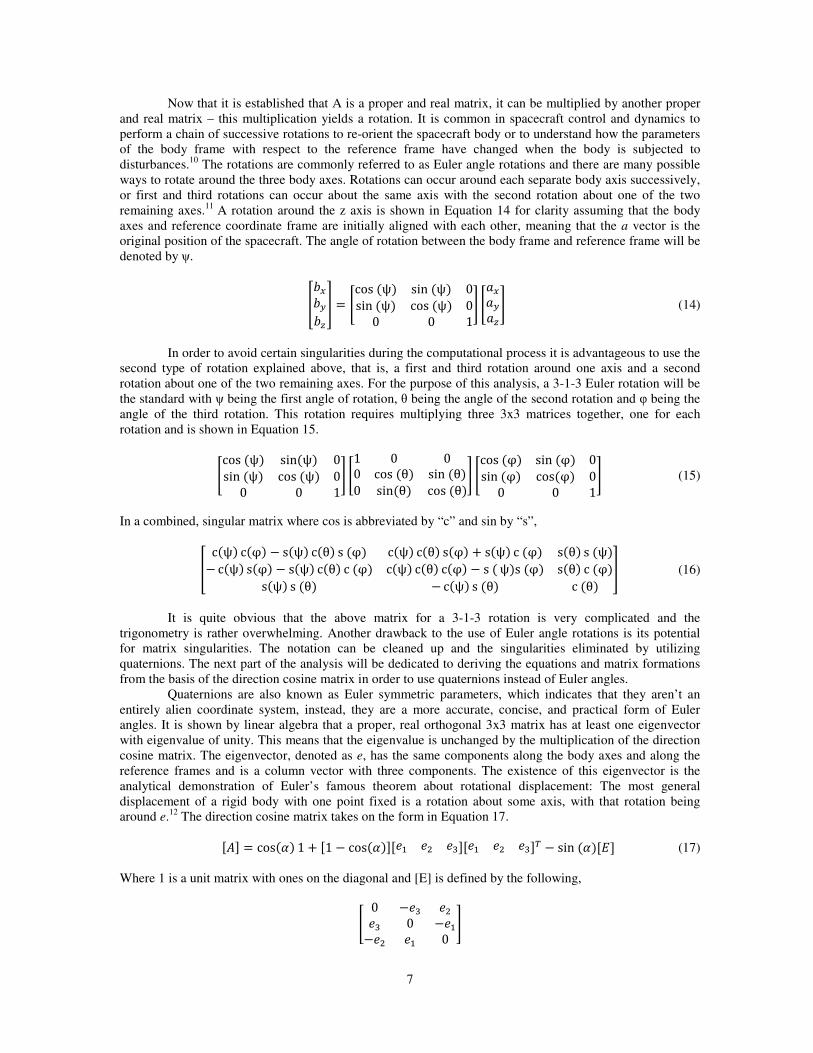
8cos ψ sinψ 0sin ψ cos ψ 00 0 1: 81 0 00 cos θ sin θ0 sinθ cos θ: 8cos φ sin φ 0sin φ cosφ 00 0 1: (15)

In a combined, singular matrix where cos is abbreviated by “c” and sin by “s”,

cψ cφ sψ cθ s φ cψ cθ sφ sψ c φ sθ s ψ cψ sφ sψ cθ c φ cψ cθ cφ s ψs φ sθ c φsψ s θ cψ s θ c θ (16)

It is quite obvious that the above matrix for a 3-1-3 rotation is very complicated and the

trigonometry is rather overwhelming. Another drawback to the use of Euler angle rotations is its potential

for matrix singularities. The notation can be cleaned up and the singularities eliminated by utilizing

quaternions. The next part of the analysis will be dedicated to deriving the equations and matrix formations

from the basis of the direction cosine matrix in order to use quaternions instead of Euler angles.

Quaternions are also known as Euler symmetric parameters, which indicates that they aren’t an

entirely alien coordinate system, instead, they are a more accurate, concise, and practical form of Euler

angles. It is shown by linear algebra that a proper, real orthogonal 3x3 matrix has at least one eigenvector

with eigenvalue of unity. This means that the eigenvalue is unchanged by the multiplication of the direction

cosine matrix. The eigenvector, denoted as e, has the same components along the body axes and along the

reference frames and is a column vector with three components. The existence of this eigenvector is the

analytical demonstration of Euler’s famous theorem about rotational displacement: The most general

displacement of a rigid body with one point fixed is a rotation about some axis, with that rotation being

around e.12

The direction cosine matrix takes on the form in Equation 17.

E9F cosG 1 E1 cosGFEH H H*FEH H H*FI sin GEJF (17)

Where 1 is a unit matrix with ones on the diagonal and [E] is defined by the following,

8 0 H* HH* 0 HH H 0 :

8

Substituting, Equation 17 becomes,

cosG H1 cosG HH1 cosG H*sin G HH*1 cosG Hsin GHH1 cosG H*sin G cosG H1 cosG HH*1 cosG Hsin GHH*1 cosG Hsin G HH*1 cosG Hsin G cosG H*1 cosG (18)

The elements of the eigenvector can be expressed as a function of the angular rotation around the

eigenvector, α, and the elements of the direction cosine matrix, with components aij, shown in Equation 18.

The three elements of the eigenvector are calculated in Equations 19-21.

H K.L2KL.MNO P (19)

H KL-2K-LMNO P (20)

H* K-.2K.-MNO P (21)

The elements of the quaternions can be expressed in terms of the principal eigenvector, e, and the

singular rotation angle around that eigenvector, α. This is shown in the next four equations.

Hsin P (22)

Hsin P (23)

* H*sin P (24)

Q cosP (25)

` There is a method by which to check the validity of the calculated quaternions that involves

summing the squares of each quaternion. The magnitude of this operation must always equal 1 (or

something very close).

* Q 1 (26)

With the key relationships developed in Equations 19-26, the direction cosine matrix from Equation

18 can be expressed in terms of quaternions that transform the spacecraft attitude from the reference frame

(old body frame) to a new body frame.

777 1 2 * 2 *Q 2* Q2 *Q 1 2 * 2* Q2* Q 2* Q 1 2 8;;; : (27)

Equations for individual quaternion values can now be determined by setting the quaternion matrix

in Equation 27 equal to the direction cosine matrix in Equation 13 as shown below. The first three elements

are computed by subtracting the off-diagonal elements from each other and the fourth element is calculated

by summing the squares of the diagonal. The algebra will be omitted for the sake of brevity and the solutions

are displayed in Equations 28-31. Note that the conversion between direction cosines and quaternions works

both ways, that is, the quaternion matrix can just as easily be converted back into a direction cosine matrix.

9

89 9 9*9 9 9*9* 9* 9**: 1 2 * 2 *Q 2* Q2 *Q 1 2 * 2* Q2* Q 2* Q 1 2

Q ST--6T..6TLL6 (28)

T.L2TL.QUV (29)

TL-2T-LQUV (30)

* T-.2T.-QUV (31)

Once again, Equation 26 is used in conjunction with Equations 28-31 to verify that the quaternions

are making correct transformations between body and reference frames. Now that there is an established

method by which to rotate and transform body axes the analysis can move forward towards understanding

how the angular rates and quaternions change with time when perturbed. This last part of the analysis will

begin by defining a few orbital parameters and then identifying the equations of motion that describe the

motion of a body under gravitational moment in a circular orbit.

The first parameter that must be established is mean motion, which is a measure of the angular

velocity of the Earth. It is a function of the gravitational parameter, µ, and the distance from the center of the

Earth, R, and is shown in Equation 32.13

W X YZL (32)

CubeSats are often injected into circular orbits around the Earth after they are launched. This type

of orbit, with a fixed radius of R and constant mean motion (Equation 32), allows the problem at hand to be

simplified and the equations of motion to become less complicated than they would otherwise be if a

CubeSat was placed in some type of eccentric orbit. The gravitational gradient torque for each axis of a

CubeSat (or any spacecraft) in the aforementioned orbit is shown in Equations 33-35. The equations are a

function of the mean motion, elements of the quaternion matrix and the principal moments of inertia.

[ *YZL 99*E F (33)

[ *YZL 99*E F (34)

[ *YZL 99E F (35)

From Equations 33-35, the angular rates for a CubeSat in a circular orbit with a fixed orbital radius

can be derived and calculated. The derivation will be omitted due to length, but the resulting coupled

differential equations will be shown. Recall the constants of proportionality originally defined in Equations

10-12 as they are directly related to the angular rate equations of the CubeSat. Like the gravitational gradient

torques, the angular rates are also dependent upon elements of the quaternion matrix, or the orientation of

the CubeSat. The angular rates are shown in Equations 36-38.

/E 3W99*F (36)

10

/E 3W9*9F (37)

/*E 3W99F (38)

In addition to the angular rates of the CubeSat changing with respect to time (and CubeSat

orientation as well), the quaternions that define the current frame of the body axes change with respect to

time and the angular rates defined in Equations 36-38. Equations 39-42 clearly illustrate this.14

E W * QF (39)

E W * QF (40)

* E WQ F (41)

Q E W* F (42)

The preceding seven equations are absolutely critical for analyzing how the CubeSat’s orientation

changes with respect to time and form the foundation of the dynamic model. Disturbances (i.e. solar

pressure, magnetic fields, etc) can be added into the model to understand how the CubeSat reacts to said

disturbances.

With the foundation of the dynamic model ready to go, keep in mind that utilizing gravity gradient

torques is a passive stabilization technique that relies solely on the Earth’s gravitational force. There may be

a need to supply additional torque to the CubeSat in the case that Earth’s gravitational force is insufficient in

minimizing disturbances, or is not supplying enough stabilization. The additional torque can be provided by

a miniature reaction wheel manufactured specifically for picosatellite applications. The inertial properties of

a reaction wheel are defined in Equation 43, where mG is the mass of the reaction wheel and rG is the radius

of the reaction wheel.15

\ ]^$. (43)

With the inertia of the reaction wheel defined, it can now be added to the dynamic model. Aligning

the center of the reaction wheel with the z-axis of the body frame (nadir pointing) and spinning around the z-

axis creates torque in the x and y directions of the body frame that can be managed by increasing or

decreasing σ, the speed of the wheel in revolutions per minute. Equations 44-46 redefine Equations 36-38

with the reaction wheel added. Note that the equation of motion for the body axis that the reaction wheel is

placed on is not affected, but due to the nature of the coupled differential equations it has an effect on the

other two body axes.

/E 3W99* _01F (44)

/E 3W9*9 _03F (45)

/*E 3W99F (46)

Recall that a significant portion of the

analysis was dedicated to understanding how

quaternions operate and can be used for this

analysis. Also recall that the conversion from

Euler angles to quaternions can be made both

ways. While the analysis was conducted using

quaternions, the following figures will be

presented in terms of yaw, pitch and roll

familiar Euler angles that are easy to visualize

and think about. Each time a set of figures

showing yaw, pitch and roll is discussed there

will be a figure showing the magnitude of the

sum of squares (Equation 26) to validate that

the Euler angles are indeed correct.

Before the figures of yaw, pitch and

roll are presented, the parameters of the

analysis will be established. The 3U CubeSat

is assumed to be in a circular orbit that has an

altitude of 500 kilometers. At this altitude, the

orbital period is 5,676.8 seconds, or 94.614

minutes. Initial values of yaw, pitch and roll

are 0 degrees, which means that the body

frame and the reference frame are initially

aligned. To understand the behavior of the

Figure 4. CAD model of a 3U

CubeSat with booms and masses

11

III. Results and Discussion

Recall that a significant portion of the

analysis was dedicated to understanding how

quaternions operate and can be used for this

analysis. Also recall that the conversion from

Euler angles to quaternions can be made both

ways. While the analysis was conducted using

quaternions, the following figures will be

h and roll – the

familiar Euler angles that are easy to visualize

and think about. Each time a set of figures

showing yaw, pitch and roll is discussed there

will be a figure showing the magnitude of the

26) to validate that

er angles are indeed correct.

Before the figures of yaw, pitch and

roll are presented, the parameters of the

analysis will be established. The 3U CubeSat

is assumed to be in a circular orbit that has an

meters. At this altitude, the

orbital period is 5,676.8 seconds, or 94.614

minutes. Initial values of yaw, pitch and roll

are 0 degrees, which means that the body

frame and the reference frame are initially

aligned. To understand the behavior of the

Figure 5. Stability chart based on principal moments of

inertia from Spacecraft Dynamics.15

Figure 6. Stability chart generated in MATLAB for a

3U CubeSat.

. CAD model of a 3U

CubeSat with booms and masses.16

. Stability chart based on principal moments of 15

. Stability chart generated in MATLAB for a

12

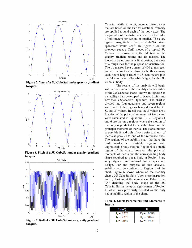
CubeSat while in orbit, angular disturbances

that are based on the Earth’s rotational velocity

are applied around each of the body axes. The

magnitudes of the disturbances are on the order

of millimeters per second or smaller. These are

typical magnitudes that a CubeSat sized

spacecraft would see.17

In Figure 4 on the

previous page, a CAD model of a typical 3U

CubeSat is shown with the addition of the

gravity gradient booms and tip masses. The

model is by no means a final design, but more

of a rough idea for the purpose of visualization.

The tip masses have a mass of 400 grams each

and are one meter apart from each other making

each boom length roughly 33 centimeters plus

the 34 centimeter allowable height for the 3U

CubeSat body The results of the analysis will begin

with a discussion of the stability characteristics

of the 3U CubeSat shape. Shown in Figure 5 is

a stability chart developed in Kane, Likins and

Levinson’s Spacecraft Dynamics. The chart is

divided into four quadrants and seven regions

with each of the regions being defined by K1,

K2 and K3 values. Recall that the K values are a

function of the principal moments of inertia and

were calculated in Equations 10-12. Regions 1

and 6 are the only regions where the motion of

the body is predicted to be stable based on the

principal moments of inertia. The stable motion

is possible if and only if each principal axis of

inertia is parallel to one of the reference axes.

The regions of the stability chart that have the

hash marks are unstable regions with

unpredictable body motion. Region 6 is a stable

region of the chart; however, the principal

moments of inertia and the corresponding body

shape required to put a body in Region 6 are

very atypical and unusual for a spacecraft

design. For the purpose of this analysis,

stability will be confined to Region 1 of the

chart. Figure 6 shows where on the stability

chart a 3U CubeSat falls. Upon close inspection

and by looking at the numbers in Table 1, the

“X” denoting the body shape of the 3U

CubeSat lies in the upper right corner of Region

1, which was previously denoted as the only

major stability region of the chart.

Table 1. Smelt Parameters and Moments of

Inertia

Figure 7. Yaw of a 3U CubeSat under gravity gradient

torques.

Figure 8. Pitch of a 3U CubeSat under gravity gradient

torques.

Figure 9. Roll of a 3U CubeSat under gravity gradient

torques.

13

Figure 6 was generated using MATLAB code, which is available for viewing in Section A of the

Appendix. The inertia values and the K values are displayed in Table 1 for reference. With the body shape of

the 3U CubeSat determined to be innately stable, the analysis can now proceed to understanding how

gravitational moments will affect the movement of the body especially when the body is perturbed.

Now that specifications, orbital

parameters and stability characteristics have

been established, the discussion can move

forward to demonstrating how gravity

gradient torques effect the body. In Figures

7, 8 and 9 the yaw, pitch and roll of a 3U

CubeSat under the effect of gravity gradient

torques are shown. For clarity, yaw is

defined as a rotation around the direction of

travel, known as the RAM direction, which

is aligned with one of the body axes. Nadir is

defined as the axis that points towards the

center of the Earth, which is aligned with the

z-body axis. Pitch is defined around the axis

that completes the right-hand rule between

the RAM direction and the Earth pointing z-

axis. Note how closely related the yaw and

pitch movements are – this is due to the

highly coupled nature of the equations of

motion (Equations 36-38). Figures 7, 8 and 9

show angular displacement of the body frame with respect to the reference frame over a 24 hour time

interval, or about 16 Earth orbits. A maximum displacement of 6 degrees from the reference frame is

observed in both yaw and pitch. The nadir direction shows an angular displacement of less than .3 degrees,

meaning that the body axis that is pointing towards the center of the Earth is maintaining high pointing

accuracy, however the motion is much more oscillatory than what is observed in yaw and pitch.

Keep in mind that the oscillatory displacements shown in Fig. 9 occur over a 24 hour period. At

first glance the figure seems to indicate that the body oscillates at a very high frequency, but when inspected

closely, there are 5 oscillations per orbital period. The oscillations in yaw and pitch are very slow and

smooth with a full oscillation taking roughly 8 hours, or about 5 orbital periods, to complete. These figures

indicate a significant amount of passive stability, which comes at no cost to the bus of the CubeSat in terms

of power expenditure for active attitude control. Figure 10 shows the sum of the squares of the quaternions

for this analysis to verify that there were no miscalculations or mistakes made. Recall from Equation 26 that

the magnitude of the sum of squares

should always be 1 as is clearly shown.

The preliminary results of the

analysis bode well for the 3U CubeSat

platform. Passive stabilization using

gravity gradient torques appears to

effectively stabilize the body. This

means that payloads requiring

moderate pointing accuracies of around

±4° (total of 8° displacement) could

feasibly be included on board the

CubeSat. Without the need for active

attitude control and the necessary

power that goes with it, there is a real

potential to include more payload

instruments on board. Including more

instruments would greatly increase scientific return. Also, take special note of the Earth pointing body axis

(nadir) in Fig. 9, which exhibits that very tight pointing accuracy. Optical sensors and small cameras could

be mounted on an Earth facing surface in conjunction with a small sensor designed to acquire pointing

knowledge (i.e. a Sun sensor) to produce high quality images from the CubeSat.

Figure 10. Quaternion magnitude check.

Figure 11. Sinclair Interplanetary miniature reaction wheels.18

14

Continuing in the vein of improving

scientific return, there is a possibility of further

stabilizing the CubeSat by using a low power

miniature reaction wheel designed specifically

for picosatellite applications. Pictured in Figure

11 is a front and side view of a fully

manufactured picosatellite reaction wheel

developed by Sinclair Interplanetary. The

reaction wheel dimensions are 50 by 50 by 30

millimeters and the total mass is .120 kilograms.

The wheel can be controlled by speed or torque

with its built-in computer. The nominal

momentum supplied by the wheel at 3410

revolutions per minute (RPM) is 10 mNm-s and

the nominal torque is 1 mNm. It’s fed by a

supply voltage ranging from 3.4V to 6V (8V

max) and is fully space qualified and tested with

diamond coated hybrid ball bearings and

redundant motor windings for increased

reliability. Additionally, it has more than two

years of flight heritage aboard the CanX-2

CubeSat mission.19

Due to the highly coupled nature of the

differential equations that govern the motion of

the body under gravity gradient torques, adding

a reaction wheel will significantly improve the

yaw, pitch and roll of the CubeSat from what

was observed in Figs. 7, 8 and 9. With the

addition of the reaction wheel, the dynamic

model will now utilize Equations 44-46 to

understand the behavior of the CubeSat. Two

possible configurations will be presented, one

with the reaction wheel providing half of the

nominal momentum (5mNm at 1705 RPM) for

a power friendly configuration that uses roughly

90 mW, the second scenario will have the

reaction wheel spinning at 3410 RPM to

generate 10mNm of momentum in a more

power hungry configuration that will use 160

mW. As a point of reference, a 3U CubeSat

can supply as much as 3W of power with its

solar cells. This reaction wheel will be using a

small fraction of the available power.

With the way the equations of motion

(Equations 39-42 and 44-46) are structured, it

is entirely possible to use just one reaction

wheel and spin it around one body axis to

obtain increased stability around all three body

axes. Figures 12, 13 and 14 will introduce the

miniature reaction wheel into the system to

understand how the behavior of the CubeSat

changes when the reaction wheel is spun. The

1705 RPM scenario will be shown first

followed by the 3410 RPM scenario. Recall

that the reaction wheel has a mass of .120

kilograms. Its calculated inertia is .00015 in4.

Figure 12. Yaw of a 3U CubeSat under gravity gradient torques

and the effect of a reaction wheel spinning at 1705 RPM.

Figure 13. Pitch of a 3U CubeSat under gravity gradient torques

and the effect of a reaction wheel spinning at 1705 RPM.

Figure 14. Roll of a 3U CubeSat under gravity gradient torques

and the effect of a reaction wheel spinning at 1705 RPM.

15

Figures 12, 13 and 14 show the yaw, pitch and roll for the power friendly reaction wheel

configuration. Figure 12 shows a maximum angular displacement of slightly less than .05 degrees in yaw

after a 24 hour period (roughly 16 orbits). The reaction wheel was able to successfully dampen the

magnitude of the oscillations from 6 degrees down to .05 degrees, as well as introduce smoothness to the

displacement curve. This is a huge improvement in stability. As with any reaction wheel, they become

saturated with momentum as time goes on. This is observed in the figures by the gradual increase in the

angular displacement. The frequency of oscillation has increased, however the displacement between the

oscillations is on the order of hundredths of a degree.

Figure 13 is the angular

displacement in pitch, which also shows a

maximum angular displacement from the

reference frame of less than .05 degrees. The

behavior of the CubeSat in the cross-track

direction is noticeably different than what is

seen in the RAM direction with large

oscillatory peaks occurring 2-3 times per

orbit. Though these spikes appear

disconcerting, they show predictable

behavior and maintain very small

magnitudes. The displacement in pitch

exhibits the same slow and gradual increase

in the magnitude of the displacement as is

observed in yaw. This is due to the

saturation of the reaction wheel, which at

some point will have to be relieved by a

momentum dumping maneuver.

Figure 14 is the angular

displacement in roll, which shows similar behavior to Fig. 13 with a total angular displacement of less than

.05 degrees and the same oscillatory spikes of small magnitude. This coupled behavior between pitch and

roll is due to the placement of the reaction wheel and the equations of motion. With the addition of the

reaction wheel spinning around the velocity vector (RAM direction), the pitch and roll receive the additional

terms in their equations of motion (Equations 44 and 45) while the equation of motion for the yaw direction

remains the same, however, its motion is still affected because of its dependency on the orientation in the

pitch and roll directions.

Figure 15 is the check on the

magnitude of the quaternions to ensure

that the analysis with the reaction wheel at

half speed is correct. The straight line with

a value of 1 in Fig. 15 indicates that there

were no errors while performing the

analysis.

The last set of figures presented

in this section will illustrate the behavior

of the CubeSat under the power hungry

reaction wheel configuration using 160

mW of power and spinning at 3410 RPM

providing 10 mNm of momentum. The

analysis was only able to run over 11

orbits due to computational intensity,

however, this does not diminish the

validity of the results. Figure 16 depicts

the angular displacement in the RAM

direction, or the yaw of the CubeSat. It is

similar in shape to the displacement

observed in Fig. 12.

Figure 15. Quaternion magnitude check.

Figure 16. Yaw of a 3U CubeSat under gravity gradient

torques and the effect of a reaction wheel spinning at 3410

RPM.

16

The maximum angular

displacement is very much the same at about

.05 degrees, though the magnitudes of the

oscillations are smaller. The extra

momentum supplied by spinning the wheel

at 3410 RPM essentially tightens everything

up. For example, in Fig. 16 at 60,000

seconds on the x-axis, there is .008 degrees

of difference between the maximum and

minimum of the oscillations. In Fig. 12 at

the same point, there is .016 degrees of

difference between oscillations. Doubling

the RPM of the reaction wheel reduced the

oscillations by 50%.

Figures 17 and 18 show the pitch

and roll of the CubeSat with the reaction

wheel spinning at 3410 RPM. As mentioned

before, the coupled differential equations

and the placement of the reaction wheel are

what make the motion in pitch and roll look

mostly the same. The motions are similar to

what is observed in Figs. 13 and 14 with the exception of the height of the peaks. They are shorter and more

round in Figs. 17 and 18, taller and thinner in Figs. 13 and 14. The change in shape is due to the increase in

wheel speed. Figure 19 is the magnitude check on the quaternions to verify the analysis integrity with the

reaction wheel at full speed.

Whether the wheel is spun at 1705 RPM or 3410 RPM, it provides significantly increased stability

characteristics on top of the natural gravity gradient torques supplied by the booms and tip masses. With less

than .05 degrees of angular displacement around all of the body axes, the motion of the CubeSat is highly

predictable and stable. Devices, sensors and optics that require high pointing accuracies of ± .5° would

flourish in this type of environment. Because of this, there is practically no limit on the type of instruments

that could be included on board the CubeSat. The expanded CubeSat platform could serve well as a test bed

for developing existing technology as well as space qualifying newly developed instruments at low cost.

There would be challenges associated with the eventual saturation of the momentum wheel and the

development of the concept of operations to dump the necessary momentum to maintain functionality,

however, this analysis was aimed only at determining the feasibility of using gravity gradient torques and the

Figure 17. Pitch of a 3U CubeSat under gravity gradient

torques and the effect of a reaction wheel spinning at

3410 RPM.

Figure 18. Roll of a 3U CubeSat under gravity gradient

torques and the effect of a reaction wheel spinning at

3410 RPM. Figure 19. Quaternion magnitude check.

17

introduction of a reaction wheel to stabilize a 3U CubeSat. The results indicate that it is not only possible,

but could prove to be the next step in seriously expanding the market for the CubeSat platform. Developing

and integrating a 3U CubeSat with gravity gradient booms and a reaction wheel, and testing the design in

microgravity, would be the path forward in this analysis.

IV. Conclusion

The results of the analysis suggest that a 3U CubeSat has every potential to be gravity gradient

stabilized. Passive stabilization yielded a maximum of 6 degrees of angular rotation around two of the body

axes and .3 degrees around the nadir pointing axis. With the addition of a small reaction wheel using only 90

mW of continuous power, the overall stability of the 3U CubeSat was dramatically increased to less than .05

degrees of angular rotation around each of the three body axes. Both of the stabilization techniques have

significant implications for the future use of CubeSats in the space industry especially in terms of

developing and qualifying instruments at low cost to the customer. As previously stated, large companies

like Northrop Grumman are starting to take advantage of the possibilities that a picosatellite platform can

offer. The interest in the CubeSat community is only going to increase as other companies examine the

potential in this opportunity. NASA has already expressed significant interest in the CubeSat program and is

developing CubeSats with Cal Poly and other state universities around the country under the ELaNA

(Educational Launch of Nanosatellite) program.

Cal Poly’s excellent reputation as a CubeSat developer and as an institution for providing launch

support with the P-POD will only help to expand the current market of customers and project opportunities.

Because of the P-POD’s minimally invasive design, it can be integrated on to many launch vehicles without

issues. As a result CubeSats can be launched much more frequently than other conventional operations

which typically take years to come to fruition.

The analysis detailed in this paper is the gateway for large and innovative design modifications to

be applied to the current standard. Testing and further analysis should continue after the publication of this

paper. With the low power requirements of the miniature reaction wheel, it would be interesting to see what

a reaction wheel placed on each body axis would do for the stability characteristics. As the functionality of

the CubeSat platform increases, the general interest in using CubeSats for research, space flight tests, and

educational purposes will literally sky rocket.

Appendix

A. MATLAB code for mass moment of inertia calculation:

% Erich Bender % AERO 463/464 -- Senior Project

%% Mass Moment of Inertia % This function roughly approximates the mass moment of inertia for a 3U % CubeSat.

function [Ix, Iy, Iz] = massmoment3U(Tmass, Tradius, Theight, Rmass,

Rlength, Bheight, Bwidth, Bdepth, Rtip1, Rtip2, Rrod1, Rrod2)

% All masses in kilograms. Heights, widths, depths and radii are in

meters.

%Inertia tensor for tip mass:

Itip = [1/12*Tmass*(3*(Tradius)^2+(Theight)^2), 0, 0; 0,

1/2*Tmass*(Tradius)^2, 0; 0, 0, 1/12*Tmass*(3*(Tradius)^2+(Theight)^2)];

%Inertia tensor for deployment rods:

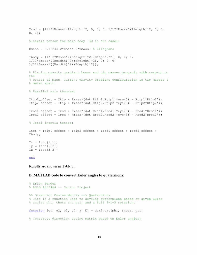
18

Irod = [1/12*Rmass*(Rlength)^2, 0, 0; 0, 1/12*Rmass*(Rlength)^2, 0; 0,

0, 0];

%Inertia tensor for main body (3U in our case):

Bmass = 3.18244-2*Rmass-2*Tmass; % kilograms

Ibody = [1/12*Bmass*((Bheight)^2+(Bdepth)^2), 0, 0; 0,

1/12*Bmass*((Bwidth)^2+(Bheight)^2), 0; 0, 0,

1/12*Bmass*((Bwidth)^2+(Bdepth)^2)];

% Placing gravity gradient booms and tip masses properly with respect to

the % center of mass. Current gravity gradient configuration is tip masses 1 % meter apart:

% Parallel axis theorem:

Itip1_offset = Itip + Tmass*(dot(Rtip1,Rtip1)*eye(3) - Rtip1*Rtip1'); Itip2_offset = Itip + Tmass*(dot(Rtip2,Rtip2)*eye(3) - Rtip2*Rtip2');

Irod1_offset = Irod + Rmass*(dot(Rrod1,Rrod1)*eye(3) - Rrod1*Rrod1'); Irod2_offset = Irod + Rmass*(dot(Rrod2,Rrod2)*eye(3) - Rrod2*Rrod2');

% Total inertia tensor:

Itot = Itip1_offset + Itip2_offset + Irod1_offset + Irod2_offset +

Ibody;

Ix = Itot(1,1); Iy = Itot(2,2); Iz = Itot(3,3);

end

Results are shown in Table 1.

B. MATLAB code to convert Euler angles to quaternions:

% Erich Bender % AERO 463/464 -- Senior Project

%% Direction Cosine Matrix --> Quaternions % This is a function used to develop quaternions based on given Euler % angles phi, theta and psi, and a full 3-1-3 rotation.

function [e1, e2, e3, e4, a, E] = dcm2quat(phi, theta, psi)

% Construct direction cosine matrix based on Euler angles:

19

DCM1 = [cosd(phi)*cosd(psi)-sind(phi)*cosd(theta)*sind(psi),

cosd(phi)*cosd(theta)*sind(psi)+sind(phi)*cosd(psi),

sind(theta)*sind(psi)];

DCM2 = [-cosd(phi)*sind(psi)-sind(phi)*cosd(theta)*cosd(psi),

cosd(phi)*cosd(theta)*cosd(psi)-sind(phi)*sind(psi),

sind(theta)*cosd(psi)];

DCM3 = [sind(phi)*sind(theta), -cosd(phi)*sind(theta), cosd(theta)];

DCM = [DCM1;DCM2;DCM3];

% Formulae for extracting quaternions out of direction cosine matrix:

e4 = .5*sqrt(DCM(1,1)+DCM(2,2)+DCM(3,3)+1); e3 = (DCM(1,2) – DCM(2,1))/(4*e4); e2 = (DCM(3,1) – DCM(1,3))/(4*e4); e1 = (DCM(2,3) – DCM(3,2))/(4*e4);

% Fundamental check on the validity of the quaternions. “a” should be

equal % to 1, or very close to it.

A = (e1)^2 + (e2)^2 + (e3)^2 + (e4)^2;

% Using the quaternion values e1, e2, e3 and e4, construct the

quaternion % matrix, E:

E1 = [(1 – 2*(e2^2+e3^2)), 2*(e1*e2 + e3*e4), 2*(e1*e3 – e2*e4)]; E2 = [2*(e1*e2 – e3*e4),(1 – 2*(e1^2+e3^2)), 2*(e2*e3 + e1*e4)]; E3 = [2*(e1*e3 + e2*e4), 2*(e2*e3 – e1*e4), (1 – 2*(e1^2+e2^2))];

E = [E1; E2; E3];

end

C. MATLAB code for the dynamic analysis:

% Erich Bender % AERO 463/464 -- Senior Project

%% Non Linear Simulation % This function utilizes ode45, quaternions and the non-linear equations

of motion to % predict angular rates of a body with supplied mass moments of inertia.

function wdot = simulation(t,x)

% Global parameters from main file:

global Ix global Iy

20

global K1 global K2 global K3

global J

% Orbital Parameters

R = 6378 + 500; %km mu = 398600; %km^3/s^2

omega = sqrt(mu/(R^3));

% Reaction Wheel rotation rate

% sigma = 0; sigma = (1705*2*pi)/(60); % RPM to rad/sec

E = [(1 – 2*(x(5)^2+x(6)^2)), 2*(x(4)*x(5) + x(6)*x(7)), 2*(x(4)*x(6) –

(x(5)*x(7))); 2*(x(4)*x(5) – x(6)*x(7)),(1 – 2*(x(4)^2+x(6)^2)),

2*(x(5)*x(6) + x(4)*x(7)); 2*(x(4)*x(6) + x(5)*x(7)), 2*(x(5)*x(6) –

x(4)*x(7)), (1 – 2*(x(4)^2 + x(5)^2))];

% Equations of motion

wdot(1) = K1*(x(2)*x(3) – 3*omega^2*E(2,1)*E(3,1)) – sigma*x(2)*(J/Ix);

% w1 wdot(2) = K2*(x(1)*x(3) – 3*omega^2*E(3,1)*E(1,1)) + sigma*x(1)*(J/Iy);

% w2 wdot(3) = K3*(x(1)*x(2) – 3*omega^2*E(1,1)*E(2,1)); % w3

wdot(4) = -.5*(-(x(3) + omega)*x(5) + x(2)*x(6) – x(1)*x(7)); %e1 wdot(5) = -.5*(-x(1)*x(6) – x(2)*x(7) + (x(3) + omega)*x(4)); %e2 wdot(6) = -.5*(x(1)*x(5) – x(2)*x(4) – (x(3) – omega)*x(7)); %e3 wdot(7) = -.5*(x(1)*x(4) + x(2)*x(5) + (x(3) – omega)*x(6)); %e4

wdot = wdot’;

end

D. MATLAB code for the main file to run the simulation:

% Erich Bender % AERO 463/464 -- Senior Project

close all clear all clc

%% Mass Moments of Inertia and Stability Chart

21

% Reference frame: The moments of inertia will be calculated along a

body % frame with: % - x pointing in the RAM direction % - y pointing in the cross-track direction to the right of the RAM % - z pointing in the Nadir direction

Tmass = .40; % tip mass (kg) Theight = .010; % height of cylindrical tip mass (m) Tradius = .015; % radius of cylindrical tip mass (m) Rmass = .010; % mass of boom (kg) Rlength = .34775; % length of boom (m) Bheight = .3405; % height of rectangular body (m) Bwidth = .10; % width of rectangular body (m) Bdepth = .10; % depth of rectangular body (m) Rtip1 = [0; 0; -.5]; % vector describing position (x,y,z) of tip mass 1

from C.M. to component in m Rtip2 = [0; 0; .5]; % vector describing position (x,y,z) of tip mass 2

from C.M. to component in m Rrod1 = [0; 0; -.335125]; % vector describing position (x,y,z) of

deployment device 1 from C.M. to component in m Rrod2 = [0; 0; .335125]; % vector describing position (x,y,z) of

deployment device 2 from C.M. to component in m

global Ix; global Iy;

[Ix, Iy, Iz] = massmoment3U(Tmass, Tradius, Theight, Rmass, Rlength,

Bheight, Bwidth, Bdepth, Rtip1, Rtip2, Rrod1, Rrod2)

global K1 K1 = ((Ix) - (Iy))/(Iz) % K1 = -.6; global K2 K2 = ((Iy) - (Iz))/(Ix) % K2 = .8824; global K3 K3 = -((K1 + K2)/(1 +K1*K2))

% Stability Chart

x1=linspace(-1,1,1000); for i=1:length(x1) y1(i)=-x1(i); end

figure(1) plot(x1,y1, K1, K2, 'xr','MarkerSize',10) axis([-1 1 -1 1]) grid off hold on line([-1,1],[0,0]) line([0,0],[-1,1]) hold off title('Stability Chart')

22

xlabel('K1') ylabel('K2')

%% Orbital Parameters

R = 6378 + 500; %km

mu = 398600; %km^3/s^2

T = ((2*pi)/sqrt(mu))*(R^(3/2)); % period in seconds

omega = sqrt(mu/(R^3)); % spin of the earth m/s

%% Initial Position (Euler Angles)

phi=0; theta=0; psi=0;

[e1i, e2i, e3i, e4i, a, E] = dcm2quat(phi, theta, psi);

%% Time Interval

ti = 0; tf = 16*T; %propagate over about 24 hours

%% Inertia Properties of Gyro/Reaction Wheel

m = .120; % kg r = .050; % m

global J J = (m*r^2)/2;

%% Gravity Gradient Simulation

x = [.01*omega, .01*omega, omega, e1i, e2i, e3i, e4i];

options=odeset('RelTol',1e-10);

[t,y]=ode45('simulation',[ti,tf],x,options);

for i = 1:length(t) e1n = y(i,4); e2n = y(i,5); e3n = y(i,6); e4n = y(i,7); a(i) = sqrt(((y(i,4))^2)+((y(i,5))^2)+((y(i,6))^2)+((y(i,7)^2))); E = [(1 - 2*(e2n^2+e3n^2)),2*(e1n*e2n + e3n*e4n),2*(e1n*e3n -

e2n*e4n);2*(e1n*e2n - e3n*e4n),(1 - 2*(e1n^2+e3n^2)),2*(e2n*e3n +

e1n*e4n);2*(e1n*e3n + e2n*e4n),2*(e2n*e3n - e1n*e4n),(1 -

2*(e1n^2+e2n^2))]; yaw(i,1)=acos(E(3,3))*180/pi;

23

pitch(i,1)=acos(E(2,2))*180/pi; roll(i,1)=acos(E(1,1))*180/pi; end

figure(2) plot(t, yaw) title('Yaw (RAM)') xlabel('Time (s)') ylabel('(deg)')

figure(3) plot(t, pitch) title('Pitch (Crosstrack)') xlabel('Time (s)') ylabel('(deg)')

figure(4) plot(t, roll) title('Roll (Nadir)') xlabel('Time (s)') ylabel('(deg)')

figure(5) plot(t,a) axis([0 tf .99 1.01]) title('Validity Check For Quaternions') xlabel('Time (s)') ylabel('Sum of the Squares')

References

1 CubeSat Project. “About Us”. URL: http://www.cubesat.org/index.php/about-us [cited 22 March 2011]

2 URL: http://www.nasa.gov/images/content/429962main_cubesat_2.jpg [cited 23 March 2011]

3 URL: http://ceng.calpoly.edu/media/uploads/articles/p-pod_300.jpg [cited 23 March 2011]

4 Department of Astronautical Engineering. “USC Nano-Satellite Blasts Off From Cape Canaveral on

SpaceX Launch”. URL: http://astronautics.usc.edu [cited 23 March 2011]

5 Hewes, Amy. “NASA Signs On with Cal Poly’s Picosatellite Deployer”. Cal Poly News. URL:

http://www.calpolynews.calpoly.edu/news_releases/2010/September/NASA.html [cited 23 March 2011]

6 URL: http://www.cubesat.org [cited 23 March 2011]

7, 8

Kraige, L. G., Meriam, J. L. Engineering Mechanics – Dynamics, 6th

Edition. John Wiley & Sons,

Inc. United States of America, 2007, pp. 556 and 665.

9, 10, 11, 12

Sidi, Marcel J. Spacecraft Dynamics & Control – A Practical Engineering Approach.

Cambridge University Press, New York, 2000, pp. 318- 320, 322-323.

13, 14, 15

Kane, T.R., Levinson, D. and Likins P.W. Spacecraft Dynamics. McGraw Hill Book Company,

San Francisco, 1983, pp. 200, 202, 241.

24

16 CAD model courtesy of Ryan Sellers.

17

CubeSat Design Specification Rev. 12, The CubeSat Program, Cal Poly - SLO. URL:

http://www.cubesat.org/images/developers/cds_rev12.pdf [cited 4 April 2011]

18, 19

Sinclair Interplanetary. Picosatellite Reaction Wheels (RW-0.01-4). URL:

http://www.sinclairinterplanetary.com/reactionwheels/10mNm-secwheel2010a.pdf [cited 5 April 2011]