an analytic solution for fractional order riccati ... solitary wave solution of a nonlinear partial...

$: An Analytic Solution for Fractional Order Riccati ... solitary wave solution of a nonlinear partial di erential ... ing the Riccati equations using fractional order ... Adomian decomposition$
Applied Mathematical Sciences, Vol. 10, 2016, no. 23, 1131 - 1150HIKARI Ltd, www.m-hikari.com

http://dx.doi.org/10.12988/ams.2016.6118

An Analytic Solution for Fractional Order

Riccati Equations by Using Optimal

Homotopy Asymptotic Method

Mohammad Hamarsheh, Ahmad Izani Ismail

School of Mathematical SciencesUniversity Sains Malaysia11800, Penang, Malaysia

Zaid Odibat

Department of Mathematics, Faculty of ScienceAl-Balqa Applied University

Al-Salt 19117, Jordan

Copyright c© 2016 Mohammad Hamarsheh et al. This article is distributed under the

Creative Commons Attribution License, which permits unrestricted use, distribution, and

reproduction in any medium, provided the original work is properly cited.

Abstract

The paper must have abstract. In this paper, we present an ap-proximate analytical algorithm to solve non-linear quadratic Riccatidifferential equations of fractional order based on the optimal homo-topy asymptotic method (OHAM). OHAM has the benefit of adjustingthe convergence rate and the region of the solution series via several aux-iliary parameters over the homotopy analysis method (HAM) that hasonly one auxiliary parameter. The proposed algorithm is applied to ini-tial value problems of the fractional order Riccati equations employingboth non-integer and integer derivatives. Additionally, our proposed al-gorithm outcomes are compared against the Adams-Bashforth-Moultonnumerical method (ABFMM) and other well-known analytical methods.

Keywords: Riccati equation, Fractional differential equation, Caputo frac-tional derivative, Optimal homotopy asymptotic method

1132 Mohammad Hamarsheh et al.

1 Introduction

An approximate analytical method is presented for the Riccati differentialequations of arbitrary order. The general form of the fractional order Riccatidifferential equation has the form

Dα∗ u(t) = A(t) +B(t)u(t) + C(t)u2(t), 0 < t ≤ T, n− 1 < α ≤ n, (1)

subject to the initial conditions

u(k)(0) = ck, k = 0, 1, . . . , n− 1, (2)

where A(t), B(t) and C(t) are given functions, ck, k = 0, 1, . . . , n − 1, arearbitrary constants, and Dα

∗ is the Caputo fractional differential operator, in-troduced in section 2, of order α.

The advantages of using fractional order differential equations in mathe-matical modelling is their non-local property. It is well-known that the integerorder differential operator is a local operator; while the fractional order dif-ferential operator is a non-local operator in that the next system state relieson its current state as well as its proceeding states. Nevertheless, becauseof several inherent differences between integer order differential equation andfractional order differential equation, many methods that are available to solvethe integer order differential equations are unsuitable for the fractional orderdifferential equations [6].

Variations of Eq. (1), with different orders, play a significant role in numer-ous applications. The solitary wave solution of a nonlinear partial differentialequation [9] and the one dimensional static Schrodinger equation [23] are ad-dressed by employing Riccati differential equations using integer order deriva-tives. Many classical and modern dynamic systems were modelled incorporat-ing the Riccati equations using fractional order derivatives [11, 20, 27]. Severalapplied science and engineering applications; including robust stabilization,network synthesis, diffusion problems, optimal filtering, controls, stochastictheory and financial mathematics, have involved the use of Riccati differentialequations [5, 7, 16, 32, 36].

There are several methods that are used to solve fractional order Ric-cati differential equations, such as Adomian decomposition method (ADM)[2], variational iteration method (VIM) [1], homotopy perturbation method(HPM) [3, 4, 21, 34], homotopy analysis method (HAM) [8, 38], combina-tion of Laplace, Adomian decomposition and Pade approximation methods[22], Taylor matrix method [15], a combination of finite difference and Pade-variational iteration numerical scheme [37] and fractional variational iteration

Fractional order Riccati equations 1133

method (FVIM) [31].Marinca et al. [19, 28, 29, 30] introduced a new analytical method in 2008,

namely the optimal homotopy asymptotic method (OHAM), to solve a varietyof nonlinear problems. Furthermore, they showed that HAM and HPM are par-ticular cases of OHAM. The OHAM is an approximate analytical tool methodthat is simple and straightforward and does not necessitate the presence of anylarge or small parameters; unlike the traditional perturbation techniques.TheOHAM has been successfully applied for obtaining an approximate solution offractional differential equation [18].

In this paper, a new algorithm based on the OHAM for solving the nonlin-ear Riccati differential Eq. (1) subject to the initial conditions given in (2) isproposed. Some basic definitions and important relations of fractional differ-ential equations are introduced in Section 2. A brief analysis of the numericalmethod ABFMM for solving fractional order Riccati differential equations isillustrated in Section 3. The analysis of the proposed algorithm of OHAM ispresented in Section 4. Some numerical experiments are discussed in Section5 to illustrate the superiority of OHAM over some existing methods.

2 Basic definitions and preliminaries

In this section we state some definitions and results from the literature whichare relevant to our work. We will adopt Caputo’s definition for the fractionalderivative which is a modification of the Riemann–Liouville definition. Thishas the advantage of being more appropriate for initial value problems in whichthe initial conditions are given in terms of the field variables and their integerorder, which is the case in most physical processes [33].

Definition 2.1 A real function f(t), t > 0 is said to be in the space Cµ (µ > 0)if it can be written as f(t) = tpf1(t) for some p > µ where f1(t) is continuousin [0,∞), and it is said to be in the space Cm

µ iff fm ∈ N ∪ 0 [24].

Definition 2.2 The Riemann-Liouville fractional integral operator (Jα) of or-der α ≥ 0, of a function f ∈ Cµ, µ ≥ −1, is defined as [17]

Jαf(t) =1

Γ(α)

∫ t

0

(t− τ)α−1f(τ)dτ, α > 0, t > 0,

J0f(t) = f(t),

where Γ(z) is the well-known Gamma function.

Details and properties of the operator Jα can be found in [35]. Note that: Forf ∈ Cµ, µ ≥ −1, α, β ≥ 0 and λ > −1, we have


• JαJβf(t) = Jα+βf(t),

• JαJβf(t) = JβJαf(t),

• Jαtλ = Γ(λ+1)Γ(λ+1+α)

tλ+α.

Definition 2.3 Let f ∈ Cm−1, m ∈ N ∪ 0. Then the Caputo fractional

derivative of f of order α > 0 is defined as [17, 25, 26]

Dα∗ f(t) = Jm−αf (m)(t) =

1

Γ(m− α)

∫ t

0

(t− τ)m−α−1f (m)(τ)dτ, t > 0,

where m− 1 < α ≤ m.

For m− 1 < α ≤ m, m ∈ N , and f, g ∈ Cmµ , µ ≥ −1, the following properties

hold [35]

• Dα∗ (af(t) + bg(t)) = aDα

∗ f(t) + bDα∗ g(t), a, b ∈ R,

• Dα∗ J

αf(t) = f(t),

• JαDα∗ f(t) = f(t)−

∑k−1j=0 f

(j)(0) tj

j!, t > 0.

3 Adams-Bashforth-Moulton method

Here we introduce the Adams-Bashforth-Moulton method (ABFMM) [12, 13]which is based on the predictor-corrector scheme [12, 10] to solve the Riccatiequation for non-integer order. Results of this method are used as a benchmarkfor comparison in our study. Let us write Eq. (1) as

Dαu(t) = r(t, u(t)) 0 < t ≤ T, (3)


u(k)(0) = ck, k = 0, 1, . . . , dαe − 1,

where r(t, u(t)) = A(t)+B(t)u(t)+C(t)u2(t). The above fractional differentialequation is equivalent to the Volterra integral equation [14]

u(t) =

dαe−1∑k=0

cktk

k!+

1

Γ(α)

∫ t

0

(t− τ)α−1r(τ, u(τ))dτ. (4)


The step size is equally spaced i.e. h = T/N where tn = nh for n = 0, 1, . . . , N .Then Eq. (4) can be rewritten in the updated form as follows

u(tn+1) =

dαe−1∑k=0

cktk

k!+

hα

Γ(α + 2)

(r(tn+1, u

p(tn+1) +n∑j=0

aj,n+1r(tj, u(tj))

),

(5)where aj,n+1 and up(tn+1) are given by

aj,n+1 =

nα+1 − (n− α)(n+ 1)α, j = 0(n− j + 2)α+1 + (n− j)α+1 − 2(n− j + 1)α+1, 1 ≤ j ≤ n1, j = n+ 1

up(tn+1) =

dαe−1∑k=0

cktk

k!+

1

Γ(α)

n∑j=0

bj,n+1r(tj, u(tj),

and

bj,n+1 =hα

α((n+ 1− j)α − (n− j)α) .

The error of this approximation is of order p, which is given by the followingexpression:

o(hp) = maxj=0,1,...,N

|u(tj)− u(tj)|,

where, p = min(2, 1 + α).

4 Analysis of the method

The OHAM was introduced and developed by Marinca et al. [29, 19, 28, 30].This method is a modification of the HAM which is based on minimizing theresidual error. In OHAM, the control and adjustment of the convergence regionare conveniently provided.

Now, we apply the OHAM to the following nonlinear fractional differentialequation

A(u(t)) + f(t) = 0, t ∈ Ω (6)

orDα∗ u(t) +N (u(t)) + f(t) = 0, t ∈ Ω (7)


B(u,du

dt) = 0, (8)

where A = Dα∗ +N , Dα

∗ is the fractional differential operator considered as a


linear operator, N is a nonlinear operator, Ω is the problem domain, t denotesthe independent variable, u(t) is an unknown function, f(t) is a known functionand B is a boundary operator.According to OHAM, the homotopy ϕ(t; q) : Ω × [0, 1] → R is constructedwhich satisfies

(1− q)[L(ϕ(t; q) + f(t)]−H(q)[A(ϕ(t; q)) + f(t)] = 0, (9)

where q ∈ [0, 1] is an embedding parameter, H(q) is a nonzero auxiliary func-tion for q 6= 0, and H(0) = 0, ϕ(t; q) is an unknown function. By substitutingq = 0 and 1 in Eq. (9), we have ϕ(t; 0) = u0(t) and ϕ(t; 1) = u(t), respectively.Hence as q increases from 0 to 1, the solution ϕ(t; q) varies continuously fromu0(t) to the exact solution u(t).By substituting q = 0 in Eq. (9), the initial approximation u0(t) = ϕ(t; 0) isobtained as the solution of the following problem.

Dα∗ (u0(t)) + f(t) = 0, B(u0,

du0

dt) = 0. (10)

We choose the auxiliary function H(q) in the form

H(q) = qC1 + q2C2 + q3C3 + . . . , (11)

where C1, C2, C3,. . . are parameters which can be determined later. Expandingϕ(t; q, C1, C2, C3, . . .) in a Taylor series with respect to q, one has

ϕ(t; q, C1, C2, C3, · · · ) = u0(t) +∞∑i=1

ui(t, C1, C2, C3, . . .)qi. (12)

Substituting Eqs. (12) and (11) into Eq. (9) and equating the coefficient oflike powers of q, then the zero order deformation equation is obtained as givenin Eq. (10). The first and the second order deformation equations are givenby

Dα∗ (u1(t)) = C1N0(u0(t)), B(u1,

du1

dt) = 0, (13)

Dα∗ (u2(t)) = Dα

∗ (u1(t))+C2N0(u0(t))+C1[Dα∗ (u1(t))+N1(u0(t), u1(t))], B(u2,

du2

dt) = 0,

(14)

and hence, the general governing equations for uj(t) are given by

Dα∗ (uj(t)) = Dα

∗ (uj−1(t))+


CjN0(u0(t)) +

j−1∑i=1

Ci[Dα∗ (uj−i(t)) +Nj−i(u0(t), u1(t), · · · , uj−1(t))],

B(uj,dujdt

) = 0; j = 3, 4, . . . ,

(15)

where Nm(u0(t), · · · , um(t)) is the coefficient of qm, obtained by expandingN (ϕ(t; q, C1, C2, C3, . . .)) in series with respect to the embedding parameter q,

N (ϕ(t; q, C1, C2, C3, . . .)) = N0(u0(t)) +∞∑j=1

Nj(u0, u1, ..., uj)qj, (16)

where ϕ(t; q, C1, C2, C3, . . .) is given in Eq. (12). It should be noted that uj forj ≥ 0 are governed by linear equations with linear boundary conditions fromthe original problem and this can be easily solved. The convergence of theseries given in Eq. (12) depends upon the auxiliary parameters C1, C2, C3, . . ..If it converges at q = 1, we have

u(t;C1, C2, C3, . . .) = u0(t) +∞∑j=1

uj(t;C1, C2, C3, . . .). (17)

Truncating the series solution (17) at level j = m, then the approximatesolution at level m is given by

um(t, C1, C2, C3, . . . , Cm) = u0(t) +m∑i=1

ui(t, C1, C2, C3, . . . , Ci). (18)

Substituting Eq. (18) into Eq. (7), we obtain the following expression for theresidual error

R(t;C1, C2, C3, . . . , Cm) =

Dα∗ (um(t;C1, C2, C3, . . . , Cm)) +N (um(t;C1, C2, C3, . . . , Cm)) + f(t). (19)

If R = 0, then um is the exact solution. In general, such a case will not arisefor nonlinear and fractional problems. For the determination of the requiredauxiliary parameters C1, C2, C3, . . ., there are many methods such as Galerkinsmethod, the Ritz method, the least squares method and the collocation methodto find the optimal values of C1, C2, C3, . . .. Here, we apply the method of leastsquares to compute the auxiliary parameters as we find it accurate and easyto implement.In theory, at the mth order of approximation, we define the exact squareresidual error, Jm(C1, C2, C3, . . . , Cm), as

Jm(C1, C2, C3, . . . , Cm) =

∫ b

a

R2(t;C1, C2, C3, . . . , Cm)dt, (20)


where the values a and b depend on the given problem. Thus, at the givenlevel of approximation m, the corresponding optimal values of convergencecontrol parameters C1, C2, C3, . . . , Cm are obtained by minimizing the exactsquare residual error, Jm, which corresponds to the following set of n algebraicequations

∂Jm∂Ci

= 0 i = 1, 2, · · · ,m. (21)

It is interesting to point out that when these parameters are determined, thenthe mth order approximate solution given by Eq. (18) will be constructed.Further details of OHAM can be found in [29, 19, 28, 30].

5 Numerical Experiments

In this section, two examples are presented to illustrate the effectiveness of theOHAM for solving the fractional order Riccati equation.Example 1. Consider the following fractional order Riccati equation [34]

Dα∗ u(t) = −u2(t) + 1, 0 ≤ t ≤ 1, 0 < α ≤ 1, (22)

subject to the initial condition

u(0) = 0. (23)

The exact solution of the equation for α = 1 is given as

u(t) =e2t − 1

e2t + 1. (24)

In view of our algorithm based on OHAM, presented in section 3, we canconstruct the following homotopy

(1− q)(Dα∗ϕ(t; q)− 1) = H(p)[Dα

∗ϕ(t; q) + ϕ2(t; q)− 1], (25)

where

ϕ(t; q) = u0(t) +∞∑j=1

uj(t)qj, (26)

H(q) = qC1 + q2C2 + q3C3 + · · · . (27)

Substituting Eq. (26) and Eq. (27) into Eq. (25), and equating the coefficientsof the same powers of q, yields the following set of linear fractional differentialequations

q0 : Dα∗ u0(t) = 1, (28)


q1 : Dα∗ u1(t) = (1 + C1)Dα

∗ u0(t) + C1u20(t)− C1 − 1, (29)

q2 : Dα∗ u2(t) = (1 +C1)Dα

∗ u1(t) +C2Dα∗ u0(t) +C2u

20(t) + 2C2u0(t)u1(t)−C2,

(30)and so on. Applying the operator Jα to both sides of Eqs. (28)-(30) and usingthe initial condition, we obtain

u0(t) =1

Γ(α + 1)tα, (31)

u1(t;C1) =22αΓ(α + 1

2)C1√

πΓ(α + 1)Γ(3α + 1)t3α, (32)

u2(t;C1, C2) =2(2α+1)3(−3α− 1

2)√πΓ(α+ 1

2)(C21 + C1 + C2)

Γ(α+ 1)2Γ(α+ 13)Γ(α+ 2

3)t3α

+2(8α+4)3(−3α− 1

2)5(−5α− 1

2)√π3Γ(α+ 1

2)Γ(2α+ 12)C2

1

Γ(α+ 1)3Γ(α+ 13)Γ(α+ 2

3)Γ(α+ 15)Γ(α+ 2

5)Γ(α+ 35)Γ(α+ 4

5)t5α. (33)

and so on. From Eq. (18), the third order approximate solution can beobtained by using the formula

u3(t) = u0(t) + u1(t;C1) + u2(t;C1, C2) + u3(t;C1, C2, C3). (34)

Table 1 shows the optimal values of the convergence control constants C1, C2,and C3 in u3(t) given in Eq. (34) for different values of α which can be obtainedusing the procedure mentioned in (19)-(21).

Table 1: Values of auxiliary parameters for the third-order OHAM solution ofEq. (22) for different orders.auxiliary parameters α = 1 α = 0.25 α = 0.5 α = 0.75 α = 0.9

C1 -0.7647692611 -0.4161392146 -0.4929758923 -0.6255388128 -0.7106697135

C2 -0.0018224597 -0.0455885997 -0.0252795594 -0.0103605496 -0.0042934878

C3 0.0000355106 -0.0070352669 -0.0042059429 -0.0011524576 -0.0002328713

Table 2 shows approximate solutions for Eq. (22), when α = 1, obtainedusing the third order OHAM solution, the exact solution given in (24), thenumerical method ABFMM [12], with h = 0.001, the fourth-component ho-motopy perturbation method (HPM) solution [34] and the eleventh-componentAdomian decomposition method (ADM) solution [1]. In Fig. 1, we plot thethird order OHAM solution, when α = 1, and the exact solution given in (24).From the numerical results shown in Fig. 1 and Table 2, we can conclude thatthe approximate solutions obtained using OHAM are in good agreement with


Table 2: Comparison of numerical results for the solution of Eq. (22) whenα = 1.

t Exact OHAM ABFMM [12] HPM [34] ADM [1]0 0.0000000000 0.0000000000 0.0000000000 0.0000000000 0.000000

0.1 0.0996679946 0.0996718794 0.0996679944 0.0996679946 0.0996670.2 0.1973753202 0.1974023559 0.1973753198 0.1973753092 0.1973750.3 0.2913126124 0.2913840225 0.2913126119 0.2913121971 0.2913120.4 0.3799489622 0.3800652965 0.3799489615 0.3799435784 0.3799480.5 0.4621171572 0.4622479172 0.4621171563 0.4620783730 0.4621170.6 0.5370495669 0.5371479432 0.5370495658 0.5368572343 0.5370490.7 0.6043677771 0.6044080838 0.6043677757 0.6036314822 0.6043670.8 0.6640367702 0.6640492005 0.6640367687 0.6617060368 0.6640370.9 0.7162978701 0.7163488085 0.7162978685 0.7099191514 0.7163001 0.7615941559 0.7616344154 0.7615941542 0.7460317460 0.761622

Table 3: Comparison of numerical results for the solution of Eq. (22), whenα = 0.25 and α = 0.5, (Error= |u3

OHAM(t)− uABFMM(t)| ).α = 0.25 α = 0.5

t OHAM ABFMM [12] HPM [34] Error OHAM ABFMM [12] HPM [34] Error0 0.000000 0.000000 0.000000 0 0.000000 0.000000 0.000000 0

0.1 0.486984 0.487151 0.334466 1.67E-04 0.331621 0.330106 0.273875 1.51E-030.2 0.538973 0.540879 0.576509 1.91E-03 0.438686 0.436835 0.454125 1.85E-030.3 0.570009 0.571773 0.738363 1.76E-03 0.505937 0.504885 0.573932 1.05E-030.4 0.592567 0.593261 0.826507 6.94E-04 0.553768 0.553779 0.644422 1.10E-050.5 0.610211 0.609616 0.848948 5.95E-04 0.590524 0.591191 0.674137 6.67E-040.6 0.624346 0.622749 0.816636 1.60E-03 0.620381 0.621011 0.671987 6.30E-040.7 0.635615 0.633677 0.743767 1.94E-03 0.645483 0.645482 0.648003 1.00E-060.8 0.644340 0.643005 0.647567 1.33E-03 0.666771 0.666016 0.613306 7.55E-040.9 0.650691 0.651121 0.547686 4.30E-04 0.684379 0.683549 0.579641 8.30E-041 0.654753 0.658290 0.465263 3.54E-03 0.697850 0.698737 0.558557 8.87E-04

exact solution for all values of t. It is clear that the overall error can be madesmaller by computing further terms using the OHAM.

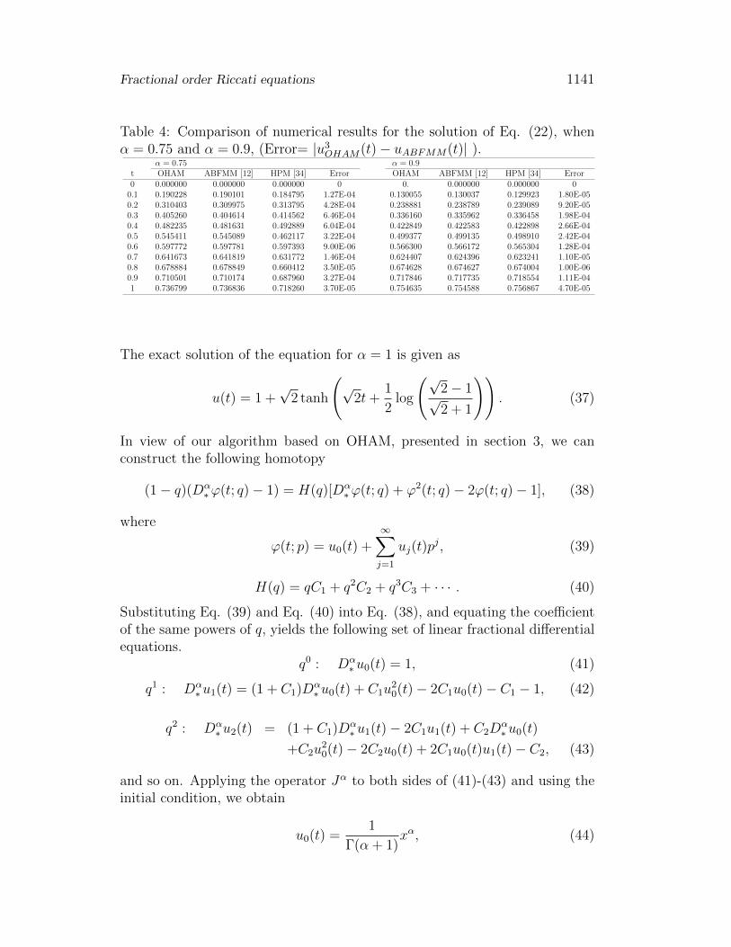
The exact solution of Eq. (22) for the fractional order case is not known,however multiple numerical solutions are available, for example, using ABFMM[12]. Tables 3 and 4 show approximate solutions for Eq. (22) using the third-order OHAM, the HPM [34] and ABFMM, with h = 0.001, for different valuesof α. From the numerical results in Tables 3 and 4, it is to be noted that theOHAM solution follows the numerical one whereas HPM needs more modifi-cation. The third order approximate solutions of Eq. (22) and the residualerrors are shown in Fig. 2 and Fig. 3, respectively, for different values of α.

Example 2. Let us consider the following fractional order Riccati equation[34]

Dα∗ u(t) = 2u(t)− u2(t) + 1, 0 ≤ t ≤ 1, 0 < α ≤ 1, (35)

u(0) = 0. (36)


Table 4: Comparison of numerical results for the solution of Eq. (22), whenα = 0.75 and α = 0.9, (Error= |u3

OHAM(t)− uABFMM(t)| ).α = 0.75 α = 0.9

t OHAM ABFMM [12] HPM [34] Error OHAM ABFMM [12] HPM [34] Error0 0.000000 0.000000 0.000000 0 0. 0.000000 0.000000 0


The exact solution of the equation for α = 1 is given as

u(t) = 1 +√

2 tanh

(√

2t+1

2log

(√2− 1√2 + 1

)). (37)

In view of our algorithm based on OHAM, presented in section 3, we canconstruct the following homotopy

(1− q)(Dα∗ϕ(t; q)− 1) = H(q)[Dα

∗ϕ(t; q) + ϕ2(t; q)− 2ϕ(t; q)− 1], (38)

where

ϕ(t; p) = u0(t) +∞∑j=1

uj(t)pj, (39)

H(q) = qC1 + q2C2 + q3C3 + · · · . (40)

Substituting Eq. (39) and Eq. (40) into Eq. (38), and equating the coefficientof the same powers of q, yields the following set of linear fractional differentialequations.

q0 : Dα∗ u0(t) = 1, (41)

q1 : Dα∗ u1(t) = (1 + C1)Dα

∗ u0(t) + C1u20(t)− 2C1u0(t)− C1 − 1, (42)

q2 : Dα∗ u2(t) = (1 + C1)Dα

∗ u1(t)− 2C1u1(t) + C2Dα∗ u0(t)

+C2u20(t)− 2C2u0(t) + 2C1u0(t)u1(t)− C2, (43)

and so on. Applying the operator Jα to both sides of (41)-(43) and using theinitial condition, we obtain

u0(t) =1

Γ(α + 1)xα, (44)


u1(t;C1) = − 2C1

Γ(2α + 1)t2α +

2(2α+1)3(−3α− 12

)√πΓ(α + 1

2)C1

Γ(α + 1)2Γ(α + 13)Γ(α + 2

3)t3α (45)

u2(x;C1, C2) = −2(C2

1 + C1 + C2)

Γ(2α+ 1)t2α

+

2(2α+1)3(−3α− 12)√πΓ(α+ 1

2)(C2

1 + C1 + C2)

Γ(α+ 1)2Γ(α+ 13

)Γ(α+ 23

)+

(8)3(−3α− 12)πC2

1

Γ(α+ 1)Γ(α+ 13

)Γ(α+ 23

)

t3α

−

2(−4α+1)3(3α+12)Γ(α+ 1

3)Γ(α+ 2

3)C2

1√πΓ(2α+ 1)2Γ(2α+ 1

2)

+2(−4α+1)√πC2

1

Γ(α+ 1)2Γ(2α+ 12

)

t4α

+2(8α+4)3(−3α− 1

2)5(−5α− 1

2)π

32 Γ(α+ 1

2)Γ(2α+ 1

2)C2

1

Γ(α+ 1)3Γ(α+ 13

)Γ(α+ 23

)Γ(α+ 15

)Γ(α+ 25

)Γ(α+ 35

)Γ(α+ 45

)t5α (46)

and so on. From Eq. (18), the third order approximate solution can beobtained by using the formula

u3(t) = u0(t) + u1(t;C1) + u2(t;C1, C2) + u3(t;C1, C2, C3). (47)

Table 5 shows the optimal values of the convergence control constants C1, C2,

Table 5: Values of auxiliary parameters for the third-order OHAM solution ofEq. (35) for different orders.auxiliary parameters α = 1 α = 0.25 α = 0.5 α = 0.75 α = 0.9

C1 -1.1359566363 -0.9902232695 -1.1755715072 1.2098520258 -1.1583109862

C2 0.2616729933 0.8471223014 1.0004637483 0.7728257720 0.4464233960

C3 -0.0609082055 -0.5151531380 -0.4650950514 -0.2417261664 -.1198033485

Table 6: Comparison of numerical results for the solution Eq. (35) when α = 1.t Exact OHAM ABFMM [12] HPM [34] VIM [1]0 0.0000000000 0.0000000000 0.0000000000 0.0000000000 0.000000

0.1 0.1102951969 0.1112136763 0.1102951933 0.1102943724 0.1102950.2 0.2419767996 0.2443164581 0.2419767925 0.2419648204 0.2419770.3 0.3951048486 0.3980915664 0.3951048385 0.3951055971 0.3951130.4 0.5678121662 0.5702708053 0.5678121542 0.5681149562 0.5678450.5 0.7560143934 0.7571636961 0.7560143809 0.7575644842 0.7560860.6 0.9535662164 0.9535657064 0.9535662047 0.9582588343 0.9536660.7 1.1529489669 1.1529057040 1.1529489566 1.163458660 1.1530370.8 1.3463636553 1.3475927635 1.3463636463 1.365239549 1.3463790.9 1.5269113132 1.5295224574 1.5269113048 1.554959751 1.5264111 1.6894983915 1.6907027573 1.6894983828 1.723809524 1.686027

and C3 in u3(t) given in Eq. (47) for different values of α which can be obtainedusing the procedure mentioned in (19)-(21). Table 6 shows approximate


Table 7: Comparison of numerical results for the solution Eq. (35), whenα = 0.25 and α = 0.5, (Error= |u3

OHAM(t)− uABFMM(t)| ).α = 0.25 α = 0.5



Table 8: Comparison of numerical results for the solution Eq. (35), whenα = 0.75 and α = 0.9, (Error= |u3

OHAM(t)− uABFMM(t)| ).α = 0.75 α = 0.9



solutions for Eq. (35), when α = 1, obtained using the third order OHAMsolution, the exact solution given in (37), the numerical method ABFMM[12], with h = 0.001, the fourth-component homotopy perturbation method(HPM) solution [34] and the third-component variational iteration method(VIM) solution [1]. In Fig. 4, we plot the third order OHAM solution, whenα = 1, and the exact solution given in (37). From the numerical results shownin Fig. 4 and Table 6, it can be concluded that the approximate solutionsobtained using OHAM are in good agreement with the exact solution for allvalues of t. Tables 7 and 8 show approximate solutions for Eq. (35) usingthe third-order OHAM, the HPM [34] and ABFMM, when h = 0.001, for thedifferent values of α. From the numerical results in Tables 7 and 8, it is clearthat the OHAM solutions are in high agreement with the ABFMM numericalsolutions. The third order approximate solutions of Eq. (35) and the residualerrors are shown in Fig. 5 and Fig. 6, respectively, for different values of α.


6 Conclusion

In this paper, we have utilized the OHAM to obtain approximate analyticalsolutions to fractional order Riccati equations. The obtained results indicatethat the OHAM could be reliable and effective tool in solving fractional differ-ential equations. The OHAM provides a simple way to control and adjust theconvergence of the series solution using the auxiliary constants Cis which areoptimally determined. Furthermore, by using different forms of the auxiliaryfunction, more accuracy can be obtained.

References

[1] S. Abbasbandy, A new application of He’s variational iteration method forquadratic Riccati differential equation by using Adomian’s polynomials,Journal of Computational and Applied Mathematics, 207 (2007), no. 1,59-63. http://dx.doi.org/10.1016/j.cam.2006.07.012

[2] S. Abbasbandy, Homotopy perturbation method for quadratic Riccatidifferential equation and comparison with Adomian’s decompositionmethod, Applied Mathematics and Computation, 172 (2006), no. 1, 485-490. http://dx.doi.org/10.1016/j.amc.2005.02.014

[3] S. Abbasbandy, Iterated He’s homotopy perturbation method forquadratic Riccati differential equation, Applied Mathematics and Com-putation, 175 (2006), no. 1, 581-589.http://dx.doi.org/10.1016/j.amc.2005.07.035

[4] H. Aminikhah, M. Hemmatnezhad, An efficient method forquadratic Riccati differential equation, Communications in Nonlin-ear Science and Numerical Simulation, 15 (2010), no. 4, 835-839.http://dx.doi.org/10.1016/j.cnsns.2009.05.009

[5] B. D. Anderson, J. B. Moore, Optimal Control: Linear Quadratic Meth-ods, Courier Corporation, 2007.

[6] V. K. Baranwal, R. K. Pandey, M. P. Tripathi, O. P. Singh, An analyticalgorithm for time fractional nonlinear reaction-diffusion equation basedon a new iterative method, Communications in Nonlinear Science andNumerical Simulation, 17 (2012), no. 10, 3906-3921.http://dx.doi.org/10.1016/j.cnsns.2012.02.015

[7] S. Brittanti, History and Prehistory of the Riccati Equation, Proceedingsof 35th IEEE Conference on Decision and Control, 2 (1996), 1599-1604.http://dx.doi.org/10.1109/cdc.1996.572758


[8] J. Cang, Y. Tan, H. Xu, S.-J. Liao, Series solutions of non-linear Riccatidifferential equations with fractional order, Chaos, Solitons and Fractals,40 (2009), no. 1, 1-9. http://dx.doi.org/10.1016/j.chaos.2007.04.018

[9] R. Conte, M. Musette, Link between solitary waves and projective Riccatiequations, Journal of Physics A: Mathematical and General, 25 (1992),no. 21, 5609-5623. http://dx.doi.org/10.1088/0305-4470/25/21/019

[10] K. Diethelm, An algorithm for the numerical solution of differential equa-tions of fractional order, Electronic Transactions on Numerical Analysis,5 (1997), no. 1, 1-6.

[11] K. Diethelm, J. M. Ford, N. J. Ford, M. Weilbeer, Pitfalls in fastnumerical solvers for fractional differential equations, Journal of Com-putational and Applied Mathematics, 186 (2006), no. 2, 482-503.http://dx.doi.org/10.1016/j.cam.2005.03.023

[12] K. Diethelm, N. J. Ford, A. D. Freed, A predictor-corrector approachfor the numerical solution of fractional differential equations, NonlinearDynamics, 29 (2002), no. 1, 3-22.http://dx.doi.org/10.1023/a:1016592219341

[13] K. Diethelm, N. J. Ford, A. D. Freed, Detailed error analysis for a frac-tional Adams method, Numerical Algorithms, 36 (2004), no. 1, 31-52.http://dx.doi.org/10.1023/b:numa.0000027736.85078.be

[14] K. Diethelm, N. J. Ford, Analysis of fractional differential equations, Jour-nal of Mathematical Analysis and Applications, 265 (2002), no. 2, 229-248.http://dx.doi.org/10.1006/jmaa.2000.7194

[15] M. Gulsu, M. Sezer, On the solution of the Riccati equation by the Taylormatrix method, Applied Mathematics and Computation, 176 (2006), no.2, 414-421. http://dx.doi.org/10.1016/j.amc.2005.09.030

[16] H. H. Goldstine, A History of the Calculus of Variations from the 17ththrough the 19th Century, vol. 5, Springer Science and Business Media,2012. http://dx.doi.org/10.1007/978-1-4613-8106-8

[17] R. Gorenflo, F. Mainardi, Fractional Calculus: Integral and Differ-ential Equations of Fractional Order, Chapter in Fractals and Frac-tional Calculus in Continuum Mechanics, Springer, 1997, 223-276.http://dx.doi.org/10.1007/978-3-7091-2664-6 5

[18] M. Hamarsheh, A. Ismail, Z. Odibat, Optimal homotopy asymptoticmethod for solving fractional relaxation-oscillation equation, Journal of


Interpolation and Approximation in Scientific Computing, 2015 (2015),no. 2, 98-111. http://dx.doi.org/10.5899/2015/jiasc-00081

[19] N. Herisanu, V. Marinca, T. Dordea, G. Madescu, A new analytical ap-proach to nonlinear vibration of an electrical machine, Proceedings of theRomanian academy, Series A, 9 (2008), no. 3, 229-236.

[20] Jiunn-Lin Wu, Chin-Hsing Chen, A new operational approach for solvingfractional calculus and fractional differential equations numerically, IE-ICE Transactions on Fundamentals of Electronics, Communications andComputer Sciences, 87 (2004), no. 5, 1077-1082.

[21] N. A. Khan, A. Ara, M. Jamil, An efficient approach for solving theRiccati equation with fractional orders, Computers and Mathematics withApplications, 61 (2011), no. 9, 2683-2689.http://dx.doi.org/10.1016/j.camwa.2011.03.017

[22] N. A. Khan, A. Ara, N. A. Khan, Fractional-order Riccati dif-ferential equation: analytical approximation and numerical re-sults, Advances in Difference Equations, 2013 (2013), no. 1, 1-16.http://dx.doi.org/10.1186/1687-1847-2013-185

[23] V. V. Kravchenko, Applied Pseudoanalytic Function Theory, Springer Sci-ence and Business Media, 2009.http://dx.doi.org/10.1007/978-3-0346-0004-0

[24] Y. F. Luchko, H. Srivastava, The exact solution of certain differen-tial equations of fractional order by using operational calculus, Com-puters and Mathematics with Applications, 29 (1995), no. 8, 73-85.http://dx.doi.org/10.1016/0898-1221(95)00031-s

[25] Y. Luchko, R. Gorenflo, The initial value problem for some fractionaldifferential equations with the Caputo derivatives, 1998.

[26] F. Mainardi, Fractional Calculus: Some Basic Problems in Con-tinuum and Statistical Mechanics, Chapter in Fractals and Frac-tional Calculus in Continuum Mechanics, Springer, 1997, 291-348.http://dx.doi.org/10.1007/978-3-7091-2664-6 7

[27] F. Mainardi, G. Pagnini, R. Gorenflo, Some aspects of fractional diffusionequations of single and distributed order, Applied Mathematics and Com-putation, 187 (2007), no. 1, 295-305.http://dx.doi.org/10.1016/j.amc.2006.08.126


[28] V. Marinca, N. Herisanu, Application of optimal homotopy asymptoticmethod for solving nonlinear equations arising in heat transfer, Inter-national Communications in Heat and Mass Transfer, 35 (2008), no. 6,710-715. http://dx.doi.org/10.1016/j.icheatmasstransfer.2008.02.010

[29] V. Marinca, N. Herisanu, C. Bota, B. Marinca, An optimal homotopyasymptotic method applied to the steady flow of a fourth-grade fluid pasta porous plate, Applied Mathematics Letters, 22 (2009), no. 2, 245-251.http://dx.doi.org/10.1016/j.aml.2008.03.019

[30] V. Marinca, N. Herisanu, I. Nemes, Optimal homotopy asymptoticmethod with application to thin film flow, Central European Journal ofPhysics, 6 (2008), no. 3, 648-653.http://dx.doi.org/10.2478/s11534-008-0061-x

[31] M. Merdan, On the solutions fractional Riccati differential equation withmodified Riemann-Liouville derivative, International Journal of Differen-tial Equations, 2012 (2012), 1-17.http://dx.doi.org/10.1155/2012/346089

[32] S. K. Mitter, Filtering and stochastic control: a historical per-spective, IEEE Control Systems Magazine, 16 (1996), no. 3, 67-76.http://dx.doi.org/10.1109/37.506400

[33] S. Momani, Z. M. Odibat, Fractional green function for linear time-fractional inhomogeneous partial differential equations in fluid mechan-ics, Journal of Applied Mathematics and Computing, 24 (2007), no. 1,167-178. http://dx.doi.org/10.1007/bf02832308

[34] Z. Odibat, S. Momani, Modified homotopy perturbation method:application to quadratic Riccati differential equation of fractionalorder, Chaos, Solitons and Fractals, 36 (2008), no. 1, 167-174.http://dx.doi.org/10.1016/j.chaos.2006.06.041

[35] I. Podlubny, Fractional Differential Equations: An Introduction to Frac-tional Derivatives, Fractional Differential Equations, to Methods of theirSolution and some of their Applications, 198, Academic Press, 1998.

[36] W. T. Reid, Riccati Differential Equations, Elsevier, 1972.

[37] N. Sweilam, M. Khader, A. Mahdy, Numerical studies for solving frac-tional Riccati differential equation, Applications and Applied Mathemat-ics, 7 (2012), no. 2, 595-608.


[38] Y. Tan, S. Abbasbandy, Homotopy analysis method for quadratic Riccatidifferential equation, Communications in Nonlinear Science and Numer-ical Simulation, 13 (2008), no. 3, 539-546.http://dx.doi.org/10.1016/j.cnsns.2006.06.006

Received: January 27, 2016; Published: March 30, 2016


Figure 1: Comparison of third-order OHAM solution and exact solu-tion in Example 1.

Figure 2: A third order OHAM solution of Eq. (22) for differentvalues of α

(a) α = 0.25 (b) α = 0.5 (c) α = 0.75 (d) α = 0.9

Figure 3: The residual errors for Eq. (22) by using 3-rd order OHAM


Figure 4: Comparison of third-order OHAM solution and exact solu-tion in Example 2.

Figure 5: A 3-rd order OHAM solution of Eq. (35) for different valuesof α

(a) α = 0.25 (b) α = 0.5 (c) α = 0.75 (d) α = 0.9

Figure 6: The residual errors for Eq. (35) by using 3-rd order OHAM

an analytic solution for fractional order riccati ... solitary wave solution of a nonlinear partial...

Documents