1

AN ANALYTICAL REAL OPTION REPLACEMENT MODEL WITH DEPRECIATION Roger Adkins* University of Salford, UK Dean Paxson** University of Manchester, UK JEL Classifications: D81, G31 Keywords: Asset replacement, two factor model, depreciation tax allowance * SBS, University of Salford, Greater Manchester, M5 4WT, UK. r.adkins@salford.ac.uk, +44 (0)1612953206. Corresponding author. ** Manchester Business School, Manchester, M15 6PB, UK.

2

AN ANALYTICAL REAL OPTION REPLACEMENT MODEL WITH DEPRECIATION Abstract A replacement model is presented for a productive asset subject to stochastic input decay, tax allowances due to a deterministic depreciation variable, and a fixed investment cost. The risk neutral valuation function is formulated and optimal trigger levels signalling replacement for the two factors is determined analytically although not as a closed-form solution. We demonstrate that the operating cost trigger level depends on asset age and increases monotonically due to positive volatility changes and that the model solution furnishes the results for certain special cases. The analysis is conducted both for a depreciation schedule specified by the declining balance and straight line method. The comparative analysis shows that although no universal ideal depreciation schedule exists between the two, the declining balance method is preferred. Finally, the solution method is sufficiently tractable to be applied in principle to real option models where time is a critical factor. 1. Introduction

The replacement policy for productive assets is normally governed by the degree of their

quality degradation, which is manifested through the stream of possible tax credits

attributable to the depreciation schedule in use as well as the operating cash flows that the

asset under study generates. For productive assets, especially those belonging to long-

lived expensive projects, these depreciation tax allowances distributed over the asset’s

lifetime can represent significant positive cash flows, which can crucially influence the

decision of whether to continue with or to replace the incumbent. By formulating these

allowances within a real option model under input decay, an analytical expression for the

optimal replacement policy is developed from the risk neutral valuation relationship so

that the extent of their significance can be evaluated.

This paper examines the replacement policy for an incumbent productive asset when the

stochastic operating cost is described by geometric Brownian motion, tax allowances due

to a deterministic depreciation variable are available and when the replacement

investment cost is fixed. The after tax risk neutral valuation relationship for the asset

value including the embedded replacement option is formulated and analytically

determined. The optimal replacement policy is then derived from the economic boundary

conditions that yield a set of simultaneous equations from which the optimal trigger

3

levels for the two focal variables are evaluated. Analysis on the stochastic replacement

model establishes that solutions to the special cases of an absent depreciation variable

and a zero underlying volatility can be derived from the general result. Numerical

analysis on the solution reveals real option model paradigm that the trigger level for the

stochastic variable and the value relationship are both increasing functions of the

underlying volatility. Since the stochastic model is constructed on two alternative

depreciation schedules, declining balance and the straight line method, a comparison is

conducted on the distinct effect of each schedule on the replacement policy to reveal that

although no depreciation schedule is universally ideal, the declining balance method is

preferred.

Fundamentally, the applications of real options methods to a decision making context in

the presence of uncertainty are founded on the valuation of perpetual American options

under risk neutrality, Samuelson (1965), and the deduction that traditional capital

budgeting techniques misprice the option value, Myers & Turnball (1976). Amongst the

original contributors to real option applications include Tourinho (1979) who values oil

shale reserves and determined the oil price trigger level signalling exploitation,

McDonald & Siegel (1985) who investigate the abandonment option, McDonald & Siegel

(1986) who demonstrate that the optimal investment policy is often to defer in the

presence of uncertainty, and Brennan & Schwartz (1985) who from deriving the optimal

conditions governing the temporary suspensions of operations and their re-enactment,

then proceed to demonstrate the effect of hysteresis.

The first investigations of stochastic replacement models are conducted using a dynamic

programming formulation, Bellman (1955), Rust (1987). Subsequent formulations seek to

identify the optimal replacement conditions when the asset degradation is described

entirely by input decay by ignoring output decay, Feldstein & Rothschild (1974), and the

operating cost uncertainty is well described by a known stochastic process. Ye (1990)

who treats the behaviour of the operating cost to be arithmetic Brownian motion,

demonstrates that the effect of uncertainty is to defer the replacement decision. Similar

results are obtained by models grounded on geometric Brownian motion. Mauer & Ott

4

(1995) devise a sophisticated formulation that is constructed on the after tax risk neutral

valuation for a replacement model involving the variations in operating cost, depreciation

and salvage price. An additional model is presented by Dobbs (2004). Other real options

models related to the productive asset replacement context include Malchow-Møller &

Thorsen (2005) on technology replacement, see also Malchow-Møller & Thorsen (2006)

and Williams (1997) on real asset redevelopment.

The present model extends the analytical scope of these real option replacement

representations by introducing the depreciation schedule as a distinct variable into the

formulation based on input decay. The introduction is completed through expressing

depreciation as a deterministic time dependent variable. This entails modelling the

depreciation variable as geometric Brownian motion with zero underlying volatility for

depreciation computed using the declining balance method and as arithmetic Brownian

motion with zero underlying volatility when using the straight line method. The

incorporation of the additional variable into the formulation means that the valuation

function for the asset including its embedded replacement option depends on two distinct

factors and that the search for the optimal trigger levels for those two factors requires the

analytical solution to a two-dimensional valuation relationship.

Previous multifactor real option models have adopted one of three methods for deriving

their results. The first approach pivots on the valuation function possessing the property

of homogeneity of degree one. Effectively, this approach treats the phenomenon under

study as an exchange option, Margrabe (1978) and Sick (1989), and uses a ratio

transformation to reduce the model dimensionality from two to one from which a closed-

form solution is generated. Illustrations of this approach include McDonald & Siegel

(1986), Williams (1991) and Malchow-Møller & Thorsen (2005). However, since the

replacement investment cost is fixed, this approach is not tenable, Adkins & Paxson

(2006). The second approach, proposed by Mauer & Ott (1995), conjectures that the

depreciation and salvage price variables can be reliably expressed as functions of the

operating cost. These substitutions entail the significant compromise that a deterministic

depreciation variable can be satisfactorily represented by a stochastic factor and that

5

salvage value is only determined by the operating cost. The third approach employs

numerical finite difference methods to solve the multi-factor valuation relationship.

Although this approach makes no compromising simplifying assumptions, it does possess

disadvantages to the method used in the present formulation. Principally, from the

method adopted here, we establish analytically the results for special cases from the

general solution. Further, it is possible in principle to derive analytical expressions for

various key indicators such as vega.

The outstanding reason for adopting the analytical procedure canvassed in this paper is

that its scope of analysis goes beyond the confines of the replacement phenomenon under

study. Since the valuation function depends on two factors, the solution method is

applicable to other two factor models for which the property of homogeneity of degree

one cannot be invoked for sound logical reasons. Secondly, the introduction of a time

dependent variable into the formulation and the analytical derivation of the resulting

valuation relationship mean that real option formulations involving a time dependent

variable should in principle be amenable to analysis and yield a quasi-analytical solution.

Potentially, this paves the way for developing and solving real option models in which

time is a critical factor such as the replacement of assets which have a finite life.

This paper is organised in the following way. In section 2, we formulate and develop the

analytical solution to the stochastic replacement real option model for an asset whose

depreciation follows a declining balance process. By modifying the parametric values, it

is demonstrated that expressions for the optimal trigger level for the operating cost is

derivable from this general model. In the following section, we conduct a variety of

simulation experiments to reveal the behaviour of the solution and to supply a greater

insight into the nature of the model. Section 4 re-examines the stochastic replacement real

option model for a straight line depreciation charge and an investigation of its sensitivity

to parametric changes is performed in the following section. A comparison of the model

results under the declining balance and straight line method is discussed in section 6. The

conclusion in section 7 brings the paper to a close. The deterministic replacement model

6

for the two variant forms of depreciation represents a benchmark for assessing the model

results and this analysis is relegated to Appendix A.

2. Replacement Opportunity with Declining Depreciation

Consider a capital asset deployed in a productive process, which has a significant bearing

on business performance. This asset suffers degradation in quality due to usage and its

degree of deterioration is reflected through increases in its operating cost. As the

operating costs for this asset become increasingly more inferior relative to those of a

newly installed replica, a decision has to be reached on whether to continue with the

incumbent asset or to replace it with a replica having a superior operating performance.

Under uncertainty, the solution for the asset replacement model is determined from

optimising the expected present value of the after tax uncertain stream of net cash flows

attributable to the asset for all possible replacement policies. The solution for the model

with a single stochastic variable is characterised by an upper critical limit, beyond which

replacement is the prescribed policy. Introducing a depreciation charge into the model,

even though it is a deterministic variable, alters the critical limit from a single point level

to a two-dimensional discriminatory boundary. The optimal policy for the replacement

model involving a stochastic operating cost variable and a deterministic depreciation

charge variable is jointly settled by their prevailing values. The discriminatory boundary,

which separates the region of continuance from replacement, is evaluated by comparing

the expected present value for the incumbent asset with that for a replica with its

improved performance less the fixed investment cost incurred from obtaining the

improvement net of any residual depreciation tax shield.

For some point of time, the operating cost for the asset under consideration is denoted by

the time dependent stochastic variable C . The notation we use in the stochastic

replacement model ignores the time subscript since its omission leads to no confusion. In

their real options analysis of capital replacement, Mauer & Ott (1995) and Dobbs (2004)

assume that the stochastic cost behaviour is adequately represented by a geometric

7

Brownian motion process with positive drift. Similarly, we will adopt the same process

by specifying the before tax operating cost as:

C C CdC Cdt Cdz= α +σ , (1)

where αC is its instantaneous drift rate, σC is the instantaneous volatility rate, and Cdz is

the increment of a standard Wiener process. The operating cost is a measure of input

decay and since the asset deteriorates with age, αC is expected to be positive.

Since the capital allowances attributed to the asset under consideration acts as a tax

shield, this factor influences the replacement decision and plays a role in determining the

discriminatory boundary. The capital allowance is represented by the depreciation charge

D , which is calculated on the basis of a declining balance and is described by a

deterministic geometric process:

DdD Ddt= −α , (2)

where αD is the constant proportional depreciation rate. Since the depreciation charge is

described deterministically by a time dependent variable then from knowing the

depreciation charge at the time of replacement, the prevailing depreciation charge level

determines the time elapsed since the last replacement.

The degradation the asset suffers is assumed to be due to input decay and impairments in

performance arising from usage are manifested in its operating cost. Output decay is

treated as not relevant for the model context and the revenues generated by the asset

under consideration remain at the constant level 0P . At the replacement event, replacing

the incumbent by a replica asset incurs a fixed known investment cost, which is denoted

by K . The replacement investment is considered to be irreversible and the asset owner is

unable to recoup any of the capital outlay on its discharge. Any salvageable value

available on discharge is assumed to be constant and is absorbed by the replacement

investment cost. If the replacement investment cost carries any instantaneous tax credits,

these are fully absorbed by K . When the incumbent is replaced by a superior replica

asset, the operating cost is restored to the superior original level 0C and the depreciation

charge level becomes 0D . If the investment cost is fully depreciable for tax purposes, 0D

8

and K are related by 0D K= θ . Although this adjustment can be accommodated in the

initial formulation, we leave it open since it is straightforward to make the refinement by

modifying the model solution.

The possession of an operating asset conveys to its owner a portfolio of options including

the option to replace. Although other operating opportunities such as changes in scale or

temporary suspension may be available, we assume that the replacement decision for the

asset under consideration is made in isolation to any other enacted policies and that these

other flexibilities are absent. We introduce the valuation function F , which is defined as

the value of the incumbent asset including its embedded replacement option. This

valuation function depends on the critical variables that influence the replacement policy.

These are the operating cost for the incumbent asset and its depreciation charge, and

( )F F C,D= . The value of the asset in use is determined in part by its attributed after tax

cash flows:

( ) ( )1− − τ + τP C D .

where τ denotes the relevant corporate tax rate. By assuming complete markets, standard

contingent claims analysis can be applied to the asset with value F to determine its risk

neutral valuation relationship as a partial differential equation (the derivation is presented

in Appendix B), Constantinides (1978), Mason & Merton (1985). The valuation

relationship is:

( )( )2

2 21C C D2 2

F F Fσ C θ C θ D P C 1 τ Dτ rF 0C C D∂ ∂ ∂

+ − + − − + − =∂ ∂ ∂

, (3)

where r denotes the risk-free rate of interest, Cθ the risk-adjusted drift rate for the

operating cost and D Dθ = α . An alternative derivation for (3) relies on using an arbitrage

argument, Shimko (1992), in which case r = µ and C Cθ = α .

The nature of F can be partly resolved by examining its behaviour as the variables

approach their limiting values. Ignoring higher derivatives greater than one, the particular

solution PF to (3) is:

9

( ) ( )0P

C D

P 1 τ C 1 τ DτFr r θ r θ− −

= − +− +

.

F , which has to be non-negative otherwise there would be no initial asset investment, is

conceived as the combination of the incumbent asset value VF and the replacement

option RF , with V RF F F= + . Since the option value is always non-negative, then VF F≥ ,

Trigeorgis (1996). Assuming an infinite lifetime:

( ) ( ) ( )0V P

C D

P 1 τ C 1 τ DτF t Fr r θ r θ− −

→ ∞ = − + =− +

.

When the operating costs for the incumbent asset become increasingly adverse and

approach infinity, there would normally exist a cogent economic justification for

replacing the incumbent. For C →∞ , the asset value becomes negative and is dominated

by the replacement option value which tends to infinity. In contrast, when the operating

costs become increasingly favourable and approach zero, no economic justification exists

for replacing the incumbent. For C 0→ , the asset value is strongly positive but the

replacement option value is close to zero. We now consider the effect of the limiting

values for the depreciation charge on the replacement option. Seemingly, we may wish to

contend that old assets are probably inefficient and ready for replacement, and so the

replacement option value is greatest when the depreciation charge tends to zero.

However, that is not the case because of the effect of the residual depreciation charge on

the replacement investment cost. Since the prevailing depreciation charge directly and

positively influences the residual depreciation tax shield, which in turn lowers the

replacement investment cost, the prevailing depreciation charge exerts its greatest

pressure on reducing the replacement investment cost when its value is at its maximum

level. This effect is palpable from the value matching relationship (8) since any reduction

in the replacement investment cost caused by the residual depreciation shield D

Dτθ

is

always greater than the present value of the depreciation tax shield in the limit D

Drτ+ θ

.

The option value for replacing the incumbent is positively influenced by the prevailing

depreciation charge and it attains its greatest value when the depreciation charge at its

10

maximum and its lowest value when it is at its minimum. Collectively, we can describe

these limiting boundary conditions by:

( ) ( ) ( ) ( )R R R RF C 0,D 0,F C ,D ,F C,D 0 0,F C,D→ → →∞ →∞ → → →∞ →∞ . (4)

The simplest kind of function satisfying (3) takes the generic form:

( ) ( )0 1 1β η − τ − τ τ

= + − +− θ + θC D

P C DF AD C

r r r, (5)

where A denotes a generic coefficient whose value is to be determined. This generic

form can be justified in two ways. Ignoring the after tax cash flow element, (3) is similar

to the valuation relationship formulated by McDonald & Siegel (1986) in their analysis of

an investment option. They express the valuation function as the solution to a two-

variable partial differential equation as a product power function. Although the partial

differential valuation relationships for the two models are not identical, (3) and theirs are

exactly the same when the variance of one variable is set to equal zero, so the solution to

their relationship with a zero variance for the relevant variable is the solution to (5).

McDonald & Siegel (1986) require that the product power function exhibits homogeneity

of degree one. We do not impose this condition on (5) and the sum of the parameters

β + η is permitted to be free. Second, (5) is the solution to (3) for the following

characteristic equation:

( ) ( )212 1 0β η = σ η η − + θ η − θ β − =C C DQ , r . (6)

This is the bivariate equivalent to the characteristic equation formulated for a single

variable model, Dixit & Pindyck (1994). Unlike the single variable case, additional

information required before the solution values for β and η can be determined. The

solutions for β and η are found from the boundary conditions. Their values are

identified by the point of intersection for the function Q and the function distilled from

the value matching relationship and associated smooth pasting condition. Since the

function Q specifies a parabola that exerts a presence in all four quadrants, the solution

values for β and η may possibly belong to any of the four quadrants, that is:

11

{ }{ }{ }{ }

1 1 1 1

2 2 2 2

3 3 3 3

4 4 4 4

I : β ,η β 0,η 0;

II : β ,η β 0,η 0;

III : β ,η β 0,η 0;

IV : β ,η β 0,η 0.

≥ ≥

≥ ≤

≤ ≥

≤ ≤

This suggests that the specific form of (5) is:

( ) ( )

i i

40β η

ii 1 C D

P 1 τ C 1 τ DτF A D Cr r θ r θ=

− −= + − +

− +∑ .

By invoking the limiting boundary conditions (4), 2 3 4A A A 0= = = and the specific

valuation function simplifies to:

( ) ( )

1 1 01

C D

P 1 C 1 DF A D Cr r r

β η − τ − τ τ= + − +

−θ + θ. (7)

The switch between assets occurs when the value of the incumbent asset attains the value

of the replica less the net replacement investment cost, where the value is determined

from the combined expected after tax net cash flow and the value of the replacement

opportunity and is specified by (7). At the replacement event, the model variables C and

D simultaneously achieve their respective trigger levels C and D . Unlike the single

variable real option models where the trigger level is represented by a single point, the

composite trigger level for the two variable model under consideration is described by an

uncountable set of paired trigger levels { }ˆ ˆC,D . There exists for this two variable model

any number of distinct trigger level possibilities because of the trade-off that exists

between the operating cost and depreciation trigger levels. If replacement is economically

viable for a specific pair of trigger levels, a small change in one trigger level

accommodated by a commensurate change in the other also satisfies the condition

conducive to optimal replacement. The uncountable set of paired trigger levels is

represented by the function G with ( )ˆ ˆG C, D 0= .

At the replacement event, the difference in the values for the incumbent and replica assets

has to equal the net replacement investment cost. The depreciation for the incumbent

12

asset at replacement is D and its residual depreciation defined as the accumulation over

its remaining life is θDD / . By assuming that the whole residual depreciation is

allowable against tax, the residual depreciation tax credit is τ θDD / and the net

replacement investment cost is − τ θDˆK D / . Similar to Mauer & Ott (1995) and Dobbs

(2004), the economic condition signaling replacement is:

( ) ( )0 0= − + τ θDˆ ˆ ˆF C,D F C ,D K D /

which can be expressed as:

( ) ( )

1 1 1 1 0 01 1 0 0

C D C D D

ˆ ˆ ˆC 1 C 1 DD DˆˆA D C A D C Kr r r r

β η β η− τ − τ ττ τ− + = − + − +

−θ + θ −θ + θ θ. (8)

Associated with the value matching relationship (8) are two smooth pasting conditions

with respect to C and D . From these, we establish that:

( )( ) ( )

1 11

1 C 1 D D

ˆ ˆ1 C rDˆˆA D C 0r r

β η − τ τ= = ≥η −θ β θ + θ

(9)

Since the option value is non-negative, 1A 0≥ , which corroborates that both 1β and 1η

are non-negative. By using (9), we eliminate 1A from (8) to yield:

( )( )

( )( ) ( )

1 100 0 0

1 11 C C D

C 1 C 1D C D1 Kˆ ˆr r rD C

β η⎛ ⎞− τ − τ τ⎛ ⎞ ⎛ ⎞η +β − + = − +⎜ ⎟⎜ ⎟ ⎜ ⎟⎜ ⎟η −θ −θ + θ⎝ ⎠ ⎝ ⎠⎝ ⎠. (10)

Since both sides of (8) have the same sign, 1 1 1β +η > .

The reduced forms of the value matching relationship and smooth pasting condition, (10)

and (9) respectively, and the characteristic equation (6) collectively constitute the model

for the value of an active productive process that embodies a replacement option to

exchange the incumbent asset with a replica. These three equations are sufficient to

determine the discriminatory boundary separating the continuance from the replacement

region. Although this model comprises four unknowns in total, C , D , 1β and 1η , the

requirement for model determinacy is satisfied since the construction of the

discriminatory boundary requires one of the variables to have a pre-specified value and

13

the function ( )ˆ ˆG C, D 0= makes up the missing equation. No closed-form analytical

solution exists for the general model and we have to resort to determining the model

solution by solving numerically the set of simultaneous equations. In the next section, we

present the simulation analysis and discuss the results that it generates.

An alternative interpretation of the reduced form value matching relationship is from

recognising that depreciation is only a time dependent variable. From (2) DT0D D e−θ=

where T denotes the elapsed time between replacements. This means that the value

matching relationship can be cast in terms of the optimal elapsed time. By replacing D

by T and eliminating C , (10) becomes:

( ) ( ) ( )

( ) ( )D

1 D 1

Tˆ 0T0 0

1 1 V1 D D C D

C 1rD e D1 e C Kr r r

−θβ θ η − ττ τ

η +β − + = − +β θ + θ −θ + θ

, (11)

where:

( ) ( )

( )D

0 1 D DV T

1 C0

1 C rC

r rD e−θ

− τ β θ + θ=

η −θτ.

The revised value matching relationship (11) and the characteristic equation (6) now form

the replacement model and by setting T to equal a pre-specified value, solutions to the

unknown parameters 1β and 1η can be determined from these two simultaneous

equations. From these values, C can be found from (9). This means that the operating

cost trigger level is time dependent and the optimal replacement policy depends on the

age of the incumbent asset. Older assets are retired and replaced by a replica at a different

operating cost trigger level than younger assets and asset usage plays a significant role in

governing the replacement policy.

By formulating the evolution of both the operating cost and depreciation, the stochastic

replacement model adopts a general form from which certain special cases can be

derived. The deterministic replacement model emerges when the volatility of the

operating cost is set to equal zero. In Appendix C, we establish that when the stochastic

14

model is constructed from applying an arbitrage approach grounded on dynamic

programming, the stochastic formulation for a zero operating cost volatility simplifies to

yield the solution to the deterministic replacement model. Second, the model presented

by Dobbs (2004) that excludes the depreciation variable from the formulation is a special

case of the general replacement model when adjustments are made to the depreciation

variable. The omission of the depreciation variable from the general replacement model

implies that Dθ is set to equal zero and the variable D is excluded from the valuation

relationship, so 1 0β = . It follows that (10) simplifies to the solution supplied by Dobbs

(2004):

( )( )

( )( )

100

11 C C

C 1 C 1C1 Kˆr rC

η⎛ ⎞− τ − τ⎛ ⎞η − + = +⎜ ⎟⎜ ⎟⎜ ⎟η −θ −θ⎝ ⎠⎝ ⎠, (12)

with:

2

C C1 11 2 22 2 2

C C C

2r⎛ ⎞ ⎛ ⎞θ θη = − + − +⎜ ⎟ ⎜ ⎟σ σ σ⎝ ⎠ ⎝ ⎠

.

A similar form to (12) is generated by modifying the definition of the residual

depreciation tax credit. By treating the residual depreciation as the discounted

depreciation accumulated over its remaining lifetime, the residual depreciation equals

( )D / µ+θ and its tax credit becomes ( )D /τ µ + θ . When this value is substituted in (8),

the depreciation trigger level D appears in the resulting value matching relationship only

through the option element and consequently, its exponent 1β is zero. The solution to the

replacement model that has a residual depreciation specified by discounting is:

( )( )

( )( )

100 0

11 C C D

C 1 C 1C D1 Kˆr r rC

η⎛ ⎞− τ − τ τ⎛ ⎞η − + = − +⎜ ⎟⎜ ⎟⎜ ⎟η −θ −θ + θ⎝ ⎠⎝ ⎠, (13)

with 1η defined as above.

Although no closed-form solution exists for the three replacement model variants, it is

possible to discern the comparative extent of the solutions they produce. Under the Dobbs

(2004) model as specified by (12), there is no residual depreciation tax credit to reduce

the replacement investment cost and its operating cost trigger level is the greatest of the

15

three since the productive asset has to operate the longest to render sufficient

compensation to balance the greatest investment cost. When the residual depreciation is

measured by its present value, the residual depreciation tax credit reduces the

replacement investment cost and consequently, the operating cost trigger level for this

model as specified by (13) is less than the level supplied by the Dobbs (2004) model.

Finally, the residual depreciation tax credit attains its greatest value for the residual

depreciation that is measured by its accumulation over its remaining potential life. This

measure consequently reduces the effective investment cost by the greatest amount and

the operating cost trigger level for this model as indicated its value matching relationship

(10) is the least amongst the three variants.

3. Simulation Results for Declining Balance Model

Further insights into the nature of the replacement model founded on the stochastic

operating cost and deterministic depreciation variable is leveraged through numerical

simulations and sensitivity analysis. Because no closed-form solution exists for the model

variants, a comparative evaluation of their properties and the identification of any

shortcomings is only achievable through the use of numerical techniques. Our primary

aim is to compare the trigger levels yielded by the models proposed by Mauer & Ott

(1995) and Dobbs (2004) relative to those produced by the present formulation. We then

proceed to penetrate the behaviour of the present formulation by examining the way the

solution changes due to variations in key variables. The numerical analysis is conducted

using the base case data that is exhibited in Table 1. This ignores the value for the

constant revenue level 0P since it is not included in the solutions. In the base case, the

initial depreciation level 0D for a replica is purposely set to equal the replacement

investment cost K adjusted by the declining balance rate Dθ with 0 DD θ K= so that

variations in these factors naturally percolate through into the computed trigger levels.

16

Table 1 Base Case Data

Replacement investment cost K 100Initial operating cost for a replica 0C 10Risk neutral operating cost drift rate Cθ 4%Operating cost volatility Cσ 25%Initial depreciation charge 0D 10Depreciation declining balance rate Dθ 10%Risk-free interest rate r 7%Relevant corporate tax rate τ 30%

The discriminatory boundaries as mapped out by the respective trigger level for the

models proposed by Mauer & Ott (1995) and Dobbs (2004) and for the present

formulation are collectively presented in Figure 1. This reveals that the discriminatory

boundary for the present formulation, which is represented by the line AB, is a declining

relationship between the respective trigger levels. The operating cost trigger level is at its

lowest value when the replica is just installed for D 10= . As the depreciation trigger

level decreases and the incumbent asset grows old, the operating cost trigger level

increases until it attains its maximum for D 0= when its age reaches infinity. The

discriminatory boundary AB distinguishes the regions of continuance and replacement.

The appropriate policy is to replace the incumbent when its prevailing operating cost and

depreciation values are located above the line AB or to continue operations with the

incumbent when otherwise.

The discriminatory boundaries for the Mauer & Ott (1995) and Dobbs (2004) models are

represented by horizontal straight lines since depreciation is respectively related to the

cost trigger level or it is ignored. For both models, the replacement region lies above its

discriminatory boundary. We know from section 2 that the discriminatory boundary for

the Dobbs (2004) model has to be situated above that for the present formulation. The

location of the Mauer & Ott (1995) discriminatory boundary relative to that for the

present formulation is obscured since it depends on the base case values. Changes in the

base case values may sufficiently lower the Mauer & Ott (1995) discriminatory boundary

17

to enable it to intersect the line AB. Notwithstanding, the model proposed by Mauer &

Ott (1995) is founded on the compromise that the deterministic depreciation variable can

be reliably represented by a function of the stochastic operating cost variable. This model

produces a discriminatory boundary that is horizontal instead of one characterised by a

declining relationship and this difference is likely to be more pronounced for younger

rather than older assets.

The profiles of 1β and 1η due to variations in the depreciation trigger level for the two

variable replacement model are presented in Figure 2. This figure reveals that the values

of both these parameters are not fixed, unlike the case for an effectively single variable

real option model, but change with the value of the depreciation trigger level. Over the

relevant range, the sum of the two parameters always exceeds one. They are increasing

functions of D , and attain their maximum levels at D 10= for a just installed asset and

their minimum levels at D 0= for an infinitely aged asset. When the asset age is infinite,

1β 0= and 1η takes on the value prescribed by the replacement model for a residual

depreciation evaluated according to its present value, (13).

4. Replacement Opportunity with Straight Line Depreciation

Since the developments of the stochastic replacement models for depreciation measured

according to the declining balance and straight line methods follow an identical structure,

we present in this section only those aspects of the analysis that are dissimilar. The

method for solving the straight line depreciation replacement model involves maximizing

the expected present value of their after tax net cash flows for all possible replacement

policies. The valuation relationship is based on risk neutrality, see Appendix B. The

solutions are described by a discriminatory boundary that separates the continuance and

replacement regions and which is found from comparing the net expected present values

for the incumbent asset and the replica. The fundamental difference between the two

models lies in the specification of the depreciation, and this has consequences for the

analysis. The remaining variables maintain their definitions from section 2.

18

The quality degradation for the asset under consideration is due to input decay and is

manifested by an operating cost evolution described by (1). Unlike declining balance

depreciation whose value does not reach zero in a finite time, straight line depreciation

introduces a complication into the formulation because of its asymmetric behaviour due

to its depletion within a finite time. When the depreciation balance is exhausted, the

depreciation level falls to zero and remains at zero until the asset is replaced. On the

installation of the replica, its cumulative depreciation CD over a notional lifetime N is

allocated evenly over its lifetime with periodic charges N CD D / N= . The remaining

cumulative depreciation charge for the asset with elapsed lifetime t is tX so 0 CX D=

and t NX 0≥ = . Straight line depreciation entails that the remaining cumulative

depreciation charge declines at the constant absolute rate ND for t N≤ :

NdX D dt= − . (14)

The value for the incumbent asset including its replacement option for straight line

depreciation is denoted by 2F , which depends on the operating costs C and the

remaining cumulative depreciation for X 0≥ or t N≤ , and from there on by only its

operating cost:

( )( )

212

22

F C, X for X 0,F

F C for X 0.

⎧ >⎪= ⎨=⎪⎩

(15)

When a zero cumulative depreciation charge is attained, the asset shares identical values

under the two regimes with ( ) ( )21 22F C, 0 F C= . Identification of the optimal replacement

policy for any time t requires that we first examine 22F and then progress to consider 21F

since its derivation depends on 22F .

For t N≥ when the remaining cumulative depreciation is zero, the straight line

depreciation replacement model reduces to the original model in the absence of

depreciation and reverts to the formulation as proposed by Dobbs (2004). This means that

the valuation function 22F for the model with straight line depreciation is:

19

( ) ( )

1 022 2

C

P 1 C 1F B C

r rη − τ − τ

= + −−θ

.

and its discriminatory boundary is specified by C in (12).

For t N< when the remaining cumulative depreciation is positive, the risk neutral

valuation relationship for 21F is:

( )( )2

2 2 21 21 211C C N 21 0 N2 2

F F Fσ C θ C D rF P C 1 τ τD 0C C X

∂ ∂ ∂+ − − + − − + =

∂ ∂ ∂. (16)

The solution to (16) is identified by splitting the partial differential equation into its

homogenous element that reflects the replacement option value and the particular element

that governs the long run asset value. The homogenous element is:

2

2 2 21 21 211C C N 212 2

F F Fσ C θ C D rF 0C C X

∂ ∂ ∂+ − − =

∂ ∂ ∂,

whose generic solution takes the form:

ψ λX21 1F B C e= .

As before, we adopt a product function as the solution to the homogenous element except

that one of its components is specified by λXe since the partial differential term with

respect to X does not involve X as a coefficient. Single variable real option models

grounded on arithmetic Brownian motion are discussed by Shimko (1992). By

substituting the solution in the homogenous element, we demonstrate that the

homogenous element is satisfied with characteristic equation:

( ) ( )212 C C N2Q ψ,λ σ ψ ψ 1 θ ψ D λ r 0= − + − − = . (17)

By adopting a similar argument as described in section 2 that explains the signs of the

exponents, we conclude that both ψ and λ are non-negative. It follows that:

1 1ψ λ X21 11F B C e= . (18)

The particular element of (16) is:

( )( )21 21C N 21 0 N

F Fθ C D rF P C 1 τ τD 0C X

∂ ∂− − + − − + =

∂ ∂, (19)

whose solution is:

20

( ) ( )0 bXN

21C

P 1 τ C 1 τ D τF aer r θ r− −

= − + +−

The unknown parameter b is found by substituting 21F in (19) to reveal that Nb r / D= − .

The complete solution to (16) is derived by stitching together the homogenous (18) and

particular elements to yield:

( ) ( )

N1 1 0 rX / Dψ λ X N21 11

C

P 1 τ C 1 τ D τF B C e aer r θ r

−− −= + − + +

−

When the remaining cumulative depreciation charge is zero, ( ) ( )21 22F C, 0 F C= . This

implies that Na τD / r= − Also when X 0= , 11 2B B= , 1 1ψ η= and 1λ 0= . It follows that:

( ) ( ) ( )N

1 1

rX / DN0ψ λ X

21 11C

D τ 1 eP 1 τ C 1 τF B C e

r r θ r

−−− −= + − +

−. (20)

The quantity N

rXD1 e

−

− is interpreted as a finite lifetime adjustment term, which equals

zero for NX D= where NX / D denotes the fraction of the remaining time before the

depreciation is fully depleted. Note that ( )NrX / DND τ 1 e / r−− represents the annuity

discounted at the risk-free rate r with a lifetime NX / D . The fundamental distinction

between the two replacement models is that the straight line variant has a finite lifetime

adjustment term to account for the eventual depletion of depreciation and the form of the

product function.

For X 0> , the remaining cumulative depreciation is positive. At the replacement event,

the difference between the values for the replica and the incumbent asset has to equal the

net replacement investment cost, where the value is determined collectively from the net

benefits. Since the remaining cumulative depreciation is denoted by X at the

replacement event and assuming that the whole amount is allowable for tax purposes, the

residual depreciation tax credit for the straight line method is ˆτX and the net replacement

investment cost becomes ˆK τX− . The value matching relationship given by

( ) ( )21 21 0 0ˆ ˆ ˆF C,X F C ,X X K= + τ − is expressed as:

21

( ) ( )

( ) ( )

N

1 1

1 01

ˆrX / DNˆψ λ X

11C

rNNλ X 0ψ

11 0C

ˆ D τ 1 eC 1 τˆB C er θ r

D τ 1 eC 1 τ ˆB C e K τX.r θ r

−

−

−−− +

−

−−= − + − +

−

(21)

The smooth pasting conditions associated with (21) is represented by:

( )( )

( )N

1 1

ˆrX / Dˆψ λ X

111 C 1

ˆ τ 1 eC 1 τˆB C eψ r θ λ

−−−= =

−. (22)

Since the replacement option element 1 1ˆψ λ X

11ˆB C e always takes on a non-negative value,

then 1ψ and 1λ are both non-negative. This corroborates our earlier conjecture. Further, a

positive change in the remaining cumulative depreciation charge produces an increase in

the replacement option value because of the presence of the residual depreciation tax

shield in the value matching condition. Using (22) to eliminate 11B from (21) yields:

( )( )

( )

( ) ( )

N1 01

1 1

ˆrX / Dλ Xψ N01 ˆψ λ X

1 C

rNN0

C

ˆ D τ 1 eC 1 τ C eψ 1 ˆψ r θ rC e

D τ 1 eC 1 τ ˆK τX.r θ r

−

−

−− ⎛ ⎞− + −⎜ ⎟− ⎝ ⎠

−−= − + −

−

(23)

The reduced forms of the value matching relationship and smooth pasting conditions,

(23) and (22) respectively, and the characteristic equation (17) collectively constitute the

valuation model for an active productive process embodying a replacement option when

depreciation is measured according to the straight line method for a positive cumulative

residual depreciation. Although the model is composed of three equations and contains

the four unknowns C , X , 1ψ , and 1λ , the model is sufficient because of the presence of

the discriminatory boundary ( )2ˆ ˆG C,X 0= . No closed-form analytical solution exists for

this model and it is necessary to recourse to numerical methods to generate the solution.

The model can be expressed in terms of T , which denotes the time elapsed between

successive replacements, by substituting C Nˆ ˆX D TD= − in (22) and (23).

22

For X 0= when the remaining cumulative depreciation is positive, the model has to be

modified to accommodate the absence of the residual depreciation tax credit and that the

installation of the replica confers a depreciation tax shield over its lifetime. At the

replacement event the value matching relationship, which is determined from

( ) ( )22 21 0 0ˆF C F C ,X K= − where 1λ 0= and 11 2B B= since X 0= , and is expressed as:

( ) ( ) ( )

12 12

rNN0ψ ψ

2 2 0C C

ˆ D τ 1 eC 1 τ C 1 τˆB C B C Kr θ r θ r

−−− −− = − + −

− −, (24)

with:

2

C C1 112 2 22 2 2

C C C

2r 1⎛ ⎞ ⎛ ⎞θ θ

ψ = − + − + ≥⎜ ⎟ ⎜ ⎟σ σ σ⎝ ⎠ ⎝ ⎠.

The associated smooth pasting condition is expressed:

( )( )

12ψ2

12 C

C 1 τˆB Cψ r θ

−=

−,

which demonstrates that 12ψ 0≥ for the replacement option element to be non-negative.

Substituting the smooth pasting condition in (24) yields:

( )( )

( ) ( )12

12

rNψN00

12 ψ12 C C

ˆ D τ 1 eC 1 τ C 1 τCψ 1 Kˆψ r θ r θ rC

−−− −⎛ ⎞− + = + − +⎜ ⎟− −⎝ ⎠

. (25)

Because the residual depreciation is depleted and X 0= , (25) supplies a single solution

value for C . This result differs from the solution proposed by Dobbs (2004) (12) by the

inclusion of the term representing the present value of the depreciation tax credit. It is

straightforward to demonstrate that the value matching relationships for this model when

X 0> and X 0= , (21) and (24) respectively, are identical for X 0= .

Finally, it is possible to demonstrate that stochastic model is general from which the

deterministic replacement solution can be derived for a zero operating cost volatility; the

proof is provided in Appendix C.

5. Simulation Results for Straight Line Method

23

We examine the effect of parametric changes on the solution results through the

application of sensitivity analysis in order to gain an insight into its behaviour.

Specifically, the investigation first evaluates the behaviour of the coefficients 1ψ , 1λ and

the cost level C signalling replacement due to changes in the prevailing remain

cumulative depreciation charge X . Then we compare the effect of alternative periodic

depreciation rates on C and contrast these with previous findings. Finally, we investigate

the impact of volatility changes on the solution. The analysis is initially performed on the

base case and then various parametric changes are introduced. The base case is specified

in Table 2.

Table 2

0C 0X K N ND τ r Cθ Cσ 40 80 100 8 10 30% 20% 15% 20%

As the previously explained method has indicated, the solution is derived from a pre-

specified value of the remaining cumulative depreciation charge X . However, we

express the behaviours in terms of the time spent since the previous re-investment T .

When the lifetime of the depreciation charge N and the initial remaining depreciation

charge 0X are set, then X determines T through 0

XT N 1X

⎛ ⎞= −⎜ ⎟⎜ ⎟

⎝ ⎠. Expressing the various

behaviours in terms of T rather than X is preferable because it is more meaningful and

enables the two regimes T N≤ and T N> to be incorporated on a single graph.

The profiles for 1ψ and 1λ , which are exhibited in Figure 7, clearly reveal the asymmetry

at the depletion event for the remaining cumulative depreciation charge, T N= . When

T N≤ , both the profiles are declining functions of T : 1λ declines to the value zero and

1ψ to 1.2846 at T N= , and they then remain at these respective values for T N> . When

the remaining cumulative depreciation charge is completely depleted, X plays no further

part in determining the optimal replacement policy. The asymmetry effect is also clearly

visible at T N= in Figure 8, which exhibits the joint behaviour of the optimal values

24

signalling replacement for the operating cost level, C and time T . The profile relating C

and T indicates the line of indifference between continuance with the incumbent asset

and its replacement. Whenever the prevailing operating cost level for a certain time since

the previous re-investment lies beneath the profile, the optimal decision is to continue

with the incumbent asset but whenever the prevailing operating cost lies above the profile

for a certain time, then the optimal decision is replacement. For T N> , the line of

indifference between continuance and replacement is independent of T since the

remaining cumulative depreciation charge is completely depleted. In contrast, there exists

a positive relationship between C and T when T N≤ . The tolerance for replacing

younger assets is less than for older assets and the degree of tolerance increases with

asset age until it reaches a maximum at the depletion event for the remaining cumulative

depreciation charge. Young machines that experience significantly high operating cost

levels will be replaced.

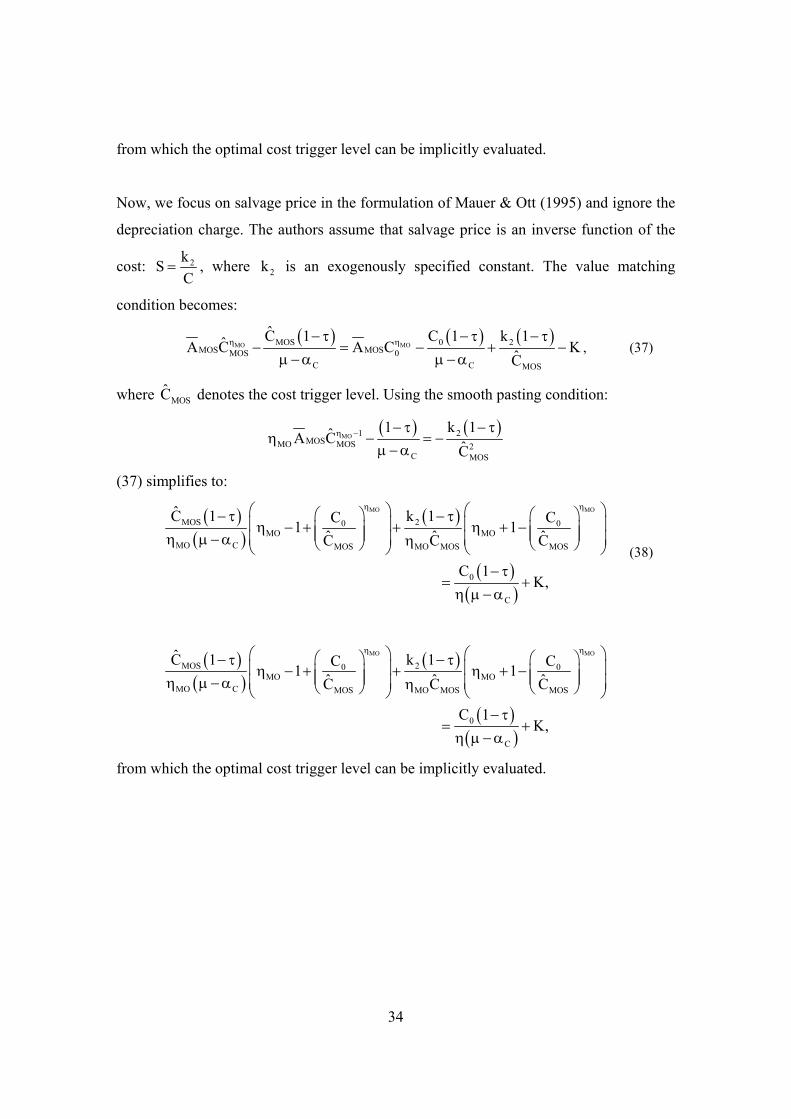
The effects of altering the depreciation lifetime for the asset are displayed in Figure 9,

which exhibits the various lines of indifference for N 20= , N 8= , N 4= and N 0= . This

figure also presents the lie of indifference for a zero depreciation amount, when

0 NX D 0= = , which is the solution to the model formulated by Dobbs (2004) and

represented by (25). When the depreciation lifetime tends to zero N 0→ , then the various

quantities involving depreciation in (21) and (23) adopt the following values:

NN 0 N

ˆD rXlim 1 exp 0r D→

⎧ ⎫⎛ ⎞⎛ ⎞τ −⎪ ⎪− →⎜ ⎟⎜ ⎟⎨ ⎬⎜ ⎟⎜ ⎟⎝ ⎠⎪ ⎪⎝ ⎠⎩ ⎭,

N 0ˆlim X 0

→τ →

and by l’Hospital’s rule:

N 00N 0 N

D rXlim 1 exp X

r D→

⎧ ⎫⎛ ⎞⎛ ⎞τ −⎪ ⎪− → τ⎜ ⎟⎨ ⎬⎜ ⎟⎜ ⎟⎝ ⎠⎪ ⎪⎝ ⎠⎩ ⎭.

As N decreases and the point of asymmetry shifts leftwards along the line of

indifference, the horizontal component to its right the reflecting (23) declines in value

while the slope of the component to its left reflecting (21) increases in value. As N

approaches zero, the component to the left of the point of asymmetry becomes

25

increasingly more insignificant and the horizontal component dominates. In contrast, as

N becomes increasingly large, then:

N 0N N

D rXlim 1 exp 0r D→∞

⎧ ⎫⎛ ⎞⎛ ⎞τ −⎪ ⎪− →⎜ ⎟⎨ ⎬⎜ ⎟⎜ ⎟⎝ ⎠⎪ ⎪⎝ ⎠⎩ ⎭

(24) and (25) are identical so the horizontal component to the right of the point of

asymmetry tends the solution value proposed by Dobbs (2004). The advantages of the

solution values yielded by Dobbs (2004) are its ease in calculation and the provision of

an upper limit. However, the present formulation demonstrates that a more efficient upper

limit is supplied by the horizontal component to the right of the point of asymmetry (24)

and that the two solution methods share a similar degree of computational ease.

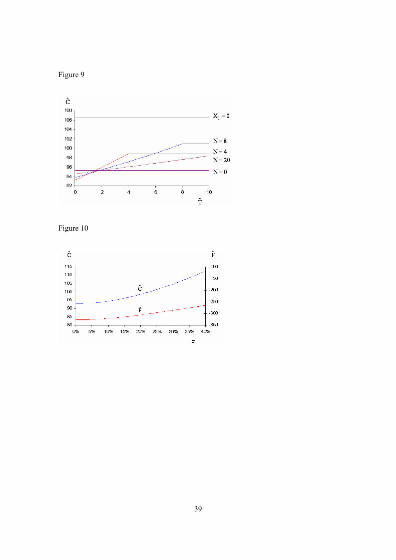
We now examine the effect of volatility changes on the solution. When C 0σ = , the

solutions for the base case to the deterministic model from (28), T 5.6315= and to the

stochastic model from (17), (21) and (22), X 23.6847= and C 93.0940= , are identical in

line with the analytical proof given in the Appendix C. It can be shown numerically that

positive changes in the volatility produce negative changes in both 1ψ and 1λ but C and

( )ˆˆ ˆF F C, X= are both increasing functions of σ . The profiles for C and F are exhibited in

Figure 10 for X 23.6847= ; in evaluating F we ignore the revenue term, which explains

its negative value. The behaviour of these profiles agree with the findings of previous

work on real options analysis and replacement models.

6. Comparison of Declining Balance and Straight Line Methods

The simulation results for the replacement real option model under declining balance and

straight line depreciation schedules presented in sections 3 and 5 respectively offer no

guidance on the comparative merits of the two alternative schedules. The aim of this

section is to compare the replacement policies for the two schedules under reasonably

similar conditions in order to identify the circumstances favouring one schedule relative

to the other and to discern whether either of the two alternatives can be classified as ideal.

Creating similar conditions underpinning the simulation exercise first requires setting the

26

variables common to both depreciation schedule to be identical. Secondly, we stipulate

that the implied expected lifetime for the incumbent asset to be set to be equal for the two

depreciation schedules. These two requirements imply that 0 DD θ K= for the declining

balance method and CD K= for the straight line method, with D1/θ N / 2= .

Table 3 Base Case Data for Comparing the Effects

of the Two Depreciation Schedules

Common Data Replacement investment cost K 100 Initial operating cost for a replica 0C 10 Risk neutral operating cost drift rate Cθ 4% Operating cost volatility Cσ 25% Risk-free interest rate r 7% Relevant corporate tax rate τ 30% Declining Balance Method Initial depreciation charge 0D 10 Depreciation declining balance rate Dθ 10% Straight Line Method Cumulative depreciation at replacement 0X 100 Length of depreciation duration N 20

In the presence of operating cost uncertainty, the comparison of the effects of the two

depreciation schedules on the replacement policy is simulated using the data presented in

Table 3. The data values for the common factors across the alternative depreciation

schedules are set to be identical. The remaining parameters, which are distinctive due to

the depreciation specification, are compelled to be comparable. The discriminatory

boundaries for the replacement model under the two depreciation schedules against the

age of the incumbent asset are presented in Figure 11.

The preferred depreciation schedule for the stochastic replacement model ought to

universally encourage the accelerated replacement of the incumbent asset relative to its

contender so that the productive process always experiences an incumbent asset that

suffers the less input decay. This criterion implies that the preferred depreciation

27

schedule ought to furnish the lower operating cost trigger level for all asset ages. Figure

11 reveals that there is no definitive winner. Although the declining balance schedule is

preferred for newly installed assets, its position changes with asset age. From

approximately 2 – 10 years, which is when the incumbent attains its expected life

according to the depreciation schedules, the straight line schedule furnishes a lower

operating cost trigger level and so represents the preferred method. The depreciation tax

allowance under the declining balance schedule continues to decline with asset age. Over

the critical range, the depreciation tax allowance for the straight line schedule becomes

relatively more pronounced as the asset ages, but its residual depreciation tax allowance

declines. The magnitude of the preference for the straight line method over this range is

not significantly large with a proportional change not exceeding 1%. When the

incumbent reaches its expected life according to the depreciation schedules, the preferred

method of depreciation reverts to declining balance. From this age onwards, the residual

depreciation tax allowance under the declining balance method becomes relatively more

pronounced and this causes comparatively accelerated replacement owing to effects on

the net replacement investment cost. Although there exists no universally ideal

depreciation method, the declining balance schedule is to be preferred since the

magnitude of the preference when it is second choice is only quite small.

7. Conclusion

In this paper, we analyse the replacement model for a productive asset that is subject to

input decay, depreciation tax allowances and a fixed investment cost. Previous real option

models on the stochastic replacement phenomenon have concentrated solely on single

factors representations. Although the model proposed by Mauer & Ott (1995) involves

three variables, these are condensed to a single variable by forcing depreciation and

salvage value to be functions of the stochastic operating cost. Real option models

specified for different contexts and involving more than a single factor either invoke the

property of homogeneity of degree one where it is logically valid in order to reduce

model dimensionality to a tractable level or resort to a purely numerical solution method.

The property of homogeneity of degree one does not hold for the formulation under

28

current study. Instead, we use an analytical approach to determining the levels triggering

replacement for the two factors by specifying the form of the valuation function and

deriving the trigger levels from the economic boundary conditions.

The quasi-analytical approach to determining the trigger levels has several comparative

advantages. We demonstrate that from the result for the general replacement model, we

can derive the special cases of a zero depreciation variable and for a zero operating cost

volatility. These derived results are shown to be identical to the single factor stochastic

replacement model under risk neutrality as proposed by Dobbs (2004) and the

deterministic model under the dynamic programming formulation. Further, it is possible

in principle to determine key indicators such as vega. The numerical results corroborate

the findings of similar past works by establishing that both the operating cost trigger level

and the valuation function increase for positive changes in the underlying volatility.

By analysing the replacement model under alternative depreciation schedules, it is

possible to discern the preferred form of schedule that comparatively accelerates the

replacement event. Although there exists no definitive victor, the schedule based on the

declining balance method is preferred for most asset ages and when it is second choice,

the difference in the operating cost trigger levels for the two methods is relatively slight.

By permitting the depreciation schedule to adopt one of two forms, a time dependent

variable is included in the formulation and the resulting valuation function depends on

two distinct factors. This two factor model is investigated through the quasi-analytical

approach which yields a set of simultaneous equations from which the trigger levels can

be generated. This approach has the potential that it can be extended to analysing multi-

factor real option models that involve a time dependent variable. This means that finite-

lived assets with embedded options, such as those whose productive life is constrained by

external obligations and natural resources, can now in principle be evaluated using this

approach.

Appendix A: Deterministic Replacement Model

29

In this appendix, we examine the replacement models in a deterministic world where the

depreciation charge is measured by (i) the declining balance and (ii) the straight line

method. The notation used here employs the subscript indexed by the time variable t

since the key variables are time dependent and the optimal solution is expressed in time

units.

(i) Declining Balance Depreciation Charge

The present value TV for an asset with a lifetime T measured in years is the discounted

future after tax net cash flows at the annualised continuous risk-adjusted rate of µ :

( ) ( ){ }C D

Tα t α t µt

T 0 0 00

V 1 τ P 1 τ C e τD e e dt− −= − − − +∫ . (26)

The asset is financially viable for some definite lifetime so Cα < µ . By adapting the

result by Lutz & Lutz (1951), the optimal replacement time for the asset is found from

maximising the value of the infinite chain V∞with respect to T , where:

( ) µTT TV V V τRD K e−= + + −∞ ∞

where TRD denotes the residual depreciation charge at replacement. Using the notation

% to represent a variable’s optimal value, the first order condition for V∞ to attain a

maximum is:

( ) TTT

T TT T

dV dRDV RD K e 0dT dT

−µ∞

==

⎛ ⎞= µ + τ − − τ =⎜ ⎟⎝ ⎠

%

%%%

. (27)

The optimal solution depends on the specification for the residual depreciation charge.

There are two alternatives. Under type A, the unused depreciation charge is granted as a

single amount allowed against tax, then TT

DRD =θ

and T*T T*

dRD DdT =

= − . (27) simplifies

to:

( ) ( )T* T*

T* 0C 0T*

C C

1 C 1 Ce De 11 D K−µ −µ− τ − τ⎛ ⎞ ⎛ ⎞α τ

+ − τ − = − +⎜ ⎟ ⎜ ⎟µ µ −α µ+ θ θ µ −α µ+θ⎝ ⎠⎝ ⎠. (28)

30

Under type B, residual depreciation allowance against tax is the present value of the

unused depreciation charges discounted at µ , then TT

DRD =µ + θ

and T

T T*

DdRDdT =

= −µ + θ

.

(27) simplifies to:

( ) ( )T*

T* 0C 0

C C

1 C 1 Ce D1 K−µ− τ − τ⎛ ⎞α τ

+ = − +⎜ ⎟µ µ −α µ−α µ+ θ⎝ ⎠. (29)

The optimal replacement time increases from type A to B because of the enhanced tax

credit on replacement.

(ii) Straight Line Depreciation Charge

Under the straight line method, the cumulative depreciation charge for capital allowance

purposes, denoted by CD , is equally apportioned over the asset’s presumed lifetime of

N . The periodic depreciation charge, ND , is given by N CD D / N= if the time point of

interest is not greater than N and ND 0= if otherwise.

When T N≤ , the present value for the asset becomes:

( ) ( ){ }C

Tα t µt

T 0 0 N0

V 1 τ P 1 τ C e τD e dt−= − − − +∫ .

The first order optimality condition is given by (27). Then under type A,

( )T NRD D N T= − with TN

dRD DdT

= − , and the optimal solution simplifies to:

( ) ( ) ( ) ( )

µT0µTT N

N

1 τ C 1 τ CτDαe1 1 e τD N T Kµ µ α µ µ α

−−⎛ ⎞− −

+ + − = − − +⎜ ⎟− −⎝ ⎠

%%% % (30)

When T N> , the present value for the asset becomes:

( ) ( ){ }0 00 0

1 1 α −µ −µ= − τ − − τ + τ∫ ∫T N

t t tT NV P C e e dt D e dt .

The value of the infinite chain becomes:

( ) −µ= + −∞ ∞T

TV V V K e .

31

And the first order optimality condition becomes:

( ) T*T

T T*

dV V K edT

−µ∞

=

= µ −

It is straightforward to derive the optimal solution:

( ) ( ) ( )T

0NT N1 C 1 CDe1 1 e K−µ

−µ⎛ ⎞− τ − ττα+ + − = +⎜ ⎟µ µ −α µ µ −α⎝ ⎠

%% . (31)

The differences between (31) and (28) are the use of N instead of T% on the left hand side

and the omission of the residual depreciation charge allowance against tax on the right

hand side.

Appendix B: Contingent Claims Analysis

Under a contingent claims formulation, a portfolio is constructed of one long unit of the

project F and ϖ short units of the operating cost C . When this portfolio is held over the

short time interval ( )t, t dt+ , it accrues a capital appreciation and cash flow gain from

its various constituents. These are shown in the following table:

F Cϖ

Capital appreciation dF dCϖ

Cash flow gain ( ) ( )( )0 1− − τ + τP C D dt Cdtϖφ

The coefficient φ represents the dividend yield for the traded security twinned with C .

Operating costs and the depreciation charge follow a geometric Brownian process (1) and

a geometric deterministic process (2) respectively. The overall gain for the portfolio over

the short time interval ( )t, t dt+ is:

( ) ( ) ( )( )1− ϖ + − − τ + τ − ϖφdF dC P C D C dt .

By invoking Ito’s lemma and setting FC∂

ϖ =∂

to eliminate terms in dZ , the overall gain

for the portfolio becomes:

32

( ) ( )2

2 212 2 1

⎛ ⎞∂ ∂ ∂σ − φ − α + − − τ + τ⎜ ⎟∂ ∂∂⎝ ⎠

D

F F FC C D P C D dt

C DC.

Since this portfolio enjoys a risk-free gain, the return on the portfolio value depends on

the risk-free rate r so:

( ) ( )2

2 212 2 1

⎛ ⎞∂ ∂ ∂ ∂⎛ ⎞− = σ − φ − α + − − τ + τ⎜ ⎟⎜ ⎟∂ ∂ ∂∂⎝ ⎠ ⎝ ⎠D

F F F Fr F C dt C C D P C D dt.

C C DC

Re-arranging, the risk neutral valuation relationship for the project F becomes:

( ) ( ) ( )2

2 212 2 1 0∂ ∂ ∂σ + − φ − α + − − τ + τ − =

∂ ∂∂ D

F F FC r C D P C D rF .

C DC (32)

When the deterministic process for the depreciation charge is arithmetic (14), the risk

neutral valuation relationship becomes:

( ) ( ) ( )2

2 212 2 1 0∂ ∂ ∂σ + − φ − α + − − τ + τ − =

∂ ∂∂ D

F F FC r C P C D rF .

C DC (33)

Except for the coefficient change, (32) and (33) are respectively identical to (3) and (16).

Appendix C

Zero variance

The stochastic model is recast within a dynamic programming framework by setting

D Dα = θ , C Cα = θ and rµ = . When C 0σ = , (6) simplifies to C 1 D 1α η −α β = µ . Further,

1 1

T0 0D C eˆ ˆD C

β η−µ⎛ ⎞ ⎛ ⎞ =⎜ ⎟ ⎜ ⎟

⎝ ⎠ ⎝ ⎠.

By making these substitutions in (10), it is straightforward to demonstrate that the

stochastic model simplifies to (28).

Mauer and Ott

Mauer & Ott (1995) treat depreciation as a function of cost and set the depreciation tax

shield over t to t dt+ equal to:

z

00

CDC

θ−

⎛ ⎞τ ⎜ ⎟

⎝ ⎠

33

where 21C C2z = α − σ . Ignoring the salvage price on disposal, their valuation relationship

is represented by the partial differential equation:

( ) ( )2

2 2 MO MO1C C 0 1 MO2 2

F FC C P 1 C 1 k C F 0C C

δ∂ ∂σ +α + − τ − − τ + τ −µ =

∂ ∂,

where 1 0 0k D C−δ= and zθ

δ = − . The solution to this partial differential equation is:

( ) ( )

MO 0 0 1MOD MOD

C

P 1 C 1 k CF A Cδ

η − τ − τ= + − +

µ µ −α Λ, (34)

where:

2

C C1 1MO 2 22 2 2

C C C

2⎛ ⎞ ⎛ ⎞α α µη = − + − +⎜ ⎟ ⎜ ⎟σ σ σ⎝ ⎠ ⎝ ⎠

,

and:

( )21C C2 1Λ = µ−α δ− σ δ δ− .

For the sake of comparison, we have ignored their reflecting barrier condition. Cancelling

out the revenue term on either side of the equation, the value matching condition

becomes:

( )

( )

MO

MO

MOD 1 MODMOD MOD

C

0 1 0 1 MODMOD 0

C

ˆ ˆC 1 k CˆA C

ˆC 1 k C k CA C K,δ δ

δη

η

− τ τ− +

µ −α Λ

− τ τ τ= − + + −

µ −α Λ θ

, (35)

where MODC represents the optimal cost trigger level under their formulation. Using the

smooth pasting condition:

( ) 1

MO

11 1 MOD 1 MOD

MO MOD MODC

ˆ ˆ1 k C k CˆA Cδ−δ−

η − − τ δ τ δ τη − + =

µ −α Λ θ.

(35) simplifies to:

( )( )

( )( )

MO

MO

0 MOD1 0 0MO

C MO C MOD

1 MOD 0MO

MO MOD

ˆˆC 1 C 1k C CK 1C

ˆk C C 1 1 ,C

ηδ

ηδ

⎛ ⎞⎛ ⎞− τ − ττ ⎜ ⎟− + = η − + ⎜ ⎟⎜ ⎟⎜ ⎟η µ −α Λ η µ −α ⎝ ⎠⎝ ⎠⎛ ⎞⎛ ⎞τ ⎛ ⎞⎜ ⎟+ η − δ + −⎜ ⎟ ⎜ ⎟⎜ ⎟⎜ ⎟η θ Λ⎝ ⎠⎝ ⎠⎝ ⎠

(36)

34

from which the optimal cost trigger level can be implicitly evaluated.

Now, we focus on salvage price in the formulation of Mauer & Ott (1995) and ignore the

depreciation charge. The authors assume that salvage price is an inverse function of the

cost: 2kSC

= , where 2k is an exogenously specified constant. The value matching

condition becomes:

( ) ( ) ( )

MO MOMOS 0 2MOS MOSMOS 0

C C MOS

C 1 C 1 k 1ˆA C A C KC

η η− τ − τ − τ− = − + −

µ −α µ −α, (37)

where MOSC denotes the cost trigger level. Using the smooth pasting condition:

( ) ( )

MO 1 2MOSMO MOS 2

C MOS

1 k 1ˆA CC

η − − τ − τη − = −

µ −α

(37) simplifies to:

( )( )

( )

( )( )

MO MO

MOS 20 0MO MO

MO C MOS MO MOS MOS

0

C

C 1 k 1C C1 1ˆ ˆ ˆC C C

C 1K,

η η⎛ ⎞ ⎛ ⎞⎛ ⎞ ⎛ ⎞− τ − τ⎜ ⎟ ⎜ ⎟η − + + η + −⎜ ⎟ ⎜ ⎟⎜ ⎟ ⎜ ⎟⎜ ⎟ ⎜ ⎟η µ −α η⎝ ⎠ ⎝ ⎠⎝ ⎠ ⎝ ⎠− τ

= +η µ −α

(38)

( )( )

( )

( )( )

MO MO

MOS 20 0MO MO

MO C MOS MO MOS MOS

0

C

C 1 k 1C C1 1ˆ ˆ ˆC C C

C 1K,

η η⎛ ⎞ ⎛ ⎞⎛ ⎞ ⎛ ⎞− τ − τ⎜ ⎟ ⎜ ⎟η − + + η + −⎜ ⎟ ⎜ ⎟⎜ ⎟ ⎜ ⎟⎜ ⎟ ⎜ ⎟η µ −α η⎝ ⎠ ⎝ ⎠⎝ ⎠ ⎝ ⎠− τ

= +η µ −α

from which the optimal cost trigger level can be implicitly evaluated.

35

Figure 1: Variations between the Operating Cost and Depreciation Trigger Levels

This figure is based on calculations using the following information:

0C 0D K Cθ Dθ r Cσ τ 10 10 100 4% 10% 7% 25% 30%

The operating cost trigger levels for the Dobbs (2004) model and the Mauer & Ott (1995) model are determined from Error! Reference source not found. and (36) respectively; the operating cost trigger level for both these formulations is independent of the depreciation trigger level. The profile of the operating cost trigger and the depreciation trigger levels for the current formulation is determined from Error! Reference source not found. and Error! Reference source not found. for the range of D from zero to 10. Typical pairs of trigger levels are presented in the following table:

D 0.0 5.0 10.0

C 32.92 31.04 29.54

36

Figure 2: Profile of the Parameters 1β and 1η for Variations in the Depreciation Trigger Level

Typical values for the parameters 1β , 1η and the depreciation trigger level D are shown in the following table:

D 1β 1η 0.0 0.0000 1.3635.0 0.0117 1.37610.0 0.0249 1.389

37

Figure 3:

38

Figure 7:

Figure 8:

39

Figure 9

Figure 10

40

Figure 11: Comparison of Operating Cost Trigger Level versus Asset Age for Depreciation

Schedules based on Declining Balance and Straight Line Method

41

References

Adkins, R., & Paxson, D. (2006). Optionality in asset renewals, Real Options

Conference. New York.

Bellman, R. E. (1955). Equipment replacement policy. Journal of the Society for

Industrial and Applied Mathematics, 3(3), 133-136.

Brennan, M. J., & Schwartz, E. S. (1985). Evaluating natural resource investments.

Journal of Business, 58(2), 135-157.

Constantinides, G. M. (1978). Market risk adjustment in project valuation. Journal of

Finance, 33(2), 603-616.

Dixit, A. K., & Pindyck, R. S. (1994). Investment under Uncertainty. Princeton (N.J.):

Princeton University Press.

Dobbs, I. M. (2004). Replacement investment: Optimal economic life under uncertainty.

Journal of Business Finance & Accounting, 31(5-6), 729-757.

Feldstein, M. S., & Rothschild, M. (1974). Towards an economic theory of replacement

investment. Econometrica, 42(3), 393-424.

Lutz, F., & Lutz, V. (1951). The Theory of Investment of the Firm. Princeton (N.J.):

Princeton University Press.

Malchow-Møller, N., & Thorsen, B. J. (2005). Repeated real options: Optimal investment

behaviour and a good rule of thumb. Journal of Economic Dynamics & Control,

29(6), 1025-1041.

Malchow-Møller, N., & Thorsen, B. J. (2006). Corrigendum to "Repeated real options:

Optimal investment behaviour and a good rule of thumb". Journal of Economic

Dynamics & Control, 30(5), 899.

Margrabe, W. (1978). The value of an option to exchange one asset for another. Journal

of Finance, 33(1), 177-186.

Mason, S. P., & Merton, R. C. (1985). The role of contingent claims analysis in corporate

finance. In E. I. Altman & M. G. Subrahmanyam (Eds.), Recent Advances in

Corporate Finance. Homewood, Illinois: Richard D. Irwin.

42

Mauer, D. C., & Ott, S. H. (1995). Investment under uncertainty: The case of replacement

investment decisions. Journal of Financial and Quantitative Analysis, 30(4), 581-

605.

McDonald, R. L., & Siegel, D. R. (1985). Investment and the valuation of firms when

there is an option to shut down. International Economic Review, 26(2), 331-349.

McDonald, R. L., & Siegel, D. R. (1986). The value of waiting to invest. The Quarterly

Journal of Economics, 101(4), 707-728.

Myers, S. C., & Turnball, S. M. (1976). Capital budgeting and the capital asset pricing

model: Good news and bad news. Journal of Finance, 32(2), 321-333.

Rust, J. (1987). Optimal replacement of GMC bus engines: An empirical model of Harold

Zurcher. Econometrica, 55(5), 999-1033.

Samuelson, P. A. (1965). Rational theory of warrant pricing. Industrial Management

Review, 6(Spring), 41-50.

Shimko, D. C. (1992). Finance in Continuous Time: A Primer. Miami: Kolb Publishing

Company.

Sick, G. (1989). Capital Budgeting with Real Options: Salomon Brothers Center for the

Study of Financial Institutions, New York University

Tourinho, O. A. F. (1979). The valuation of reserves of natural resources: an option

pricing approach: University of California, Berkeley.

Trigeorgis, L. (1996). Real Options: Managerial Flexibility and Strategy in Resource

Allocation. Cambridge (Mass.): MIT Press.

Williams, J. T. (1991). Real estate development as an option. Journal of Real Estate

Finance and Economics, 4, 191-208.

Williams, J. T. (1997). Redevelopment of real assets. Real Estate Economics, 25(3), 387-

407.

Ye, M.-H. (1990). Optimal replacement policy with stochastic maintenance and operation

costs. European Journal of Operational Research, 44, 84-94.

43