An analytical shear–lag model for composites with ‘brick–and–mortar’architecture considering non-linear matrix response and failure

Soraia Pimentaa,∗, Paul Robinsonb

aThe Composites Centre, Department of Mechanical Engineering, South Kensington Campus,Imperial College London, SW7 2AZ, United Kingdom

bThe Composites Centre, Department of Aeronautics, South Kensington Campus,Imperial College London, SW7 2AZ, United Kingdom

Abstract

Discontinuous composites can combine high stiffness and strength with ductility and dam-

age tolerance. This paper presents an analytical shear–lag model for the tensile response

of discontinuous composites with a ‘brick–and–mortar’ architecture, composed of regularly

staggered stiff platelets embedded in a soft matrix. The formulation is applicable to different

types of matrix material (e.g. brittle, perfectly–plastic, strain–hardening), which are modelled

through generic piecewise–linear and fracture–mechanics consistent shear constitutive laws.

Full composite stress–strain curves are calculated in less than 1 second, thanks to an effi-

cient implementation scheme based on the determination of process zone lengths. Parametric

studies show that the model bridges the yield–slip (plasticity) theory and fracture mechan-

ics, depending on platelet thickness, platelet aspect–ratio and matrix constitutive law. The

potential for using ‘brick–and–mortar’ architectures to produce composites which are simul-

taneously strong, stiff and ductile is discussed, and optimised configurations are proposed.

Keywords: ‘Brick–and–mortar’ architecture, B. Non-linear behaviour, C. Damage

mechanics, C. Modelling, C. Stress transfer

1. Introduction

Most natural structural materials combining high stiffness, high strength and damage

tolerance (e.g. nacre, bone and spider silk) share a common motif: a discontinuous ‘brick–

and–mortar’ architecture (see Figure 1a) with staggered stiff inclusions (e.g. fibres or platelets)

embedded in a soft matrix [1, 2]. This provides two deformation mechanisms under tension: (i)

extension of the inclusions (which dominates in the elastic domain and confers initial stiffness),

and (ii) shearing of the matrix (which promotes large deformations and energy dissipation

∗Corresponding author.Email address: soraia.pimenta@imperial.ac.uk (Soraia Pimenta)

Pimenta S, Robinson P (2014). An analytical shear–lag model for composites with ‘brick–and–mortar’ archi-tecture considering non-linear matrix response and failure. Composites Science and Technology 104, 111–124.DOI:10.1016/j.compscitech.2014.09.001

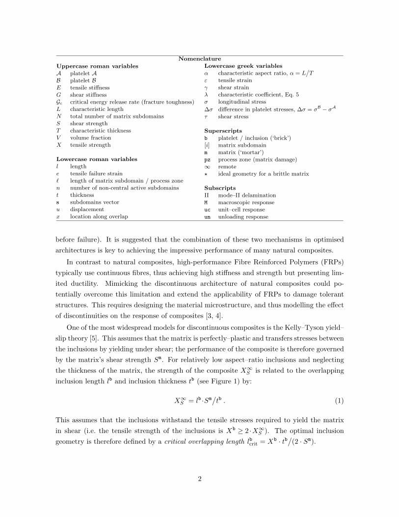
Nomenclature

Uppercase roman variablesA platelet AB platelet BE tensile stiffnessG shear stiffnessGc critical energy release rate (fracture toughness)L characteristic lengthN total number of matrix subdomainsS shear strengthT characteristic thicknessV volume fractionX tensile strength

Lowercase roman variablesl lengthe tensile failure strain` length of matrix subdomain / process zonen number of non-central active subdomainst thicknesss subdomains vectoru displacementx location along overlap

Lowercase greek variablesα characteristic aspect ratio, α = L

/T

ε tensile strainγ shear strainλ characteristic coefficient, Eq. 5σ longitudinal stress

∆σ difference in platelet stresses, ∆σ = σB − σAτ shear stress

Superscriptsb platelet / inclusion (‘brick’)[i] matrix subdomainm matrix (‘mortar’)pz process zone (matrix damage)∞ remote? ideal geometry for a brittle matrix

SubscriptsII mode–II delaminationM macroscopic responseuc unit–cell responseun unloading response

before failure). It is suggested that the combination of these two mechanisms in optimised

architectures is key to achieving the impressive performance of many natural composites.

In contrast to natural composites, high-performance Fibre Reinforced Polymers (FRPs)

typically use continuous fibres, thus achieving high stiffness and strength but presenting lim-

ited ductility. Mimicking the discontinuous architecture of natural composites could po-

tentially overcome this limitation and extend the applicability of FRPs to damage tolerant

structures. This requires designing the material microstructure, and thus modelling the effect

of discontinuities on the response of composites [3, 4].

One of the most widespread models for discontinuous composites is the Kelly–Tyson yield–

slip theory [5]. This assumes that the matrix is perfectly–plastic and transfers stresses between

the inclusions by yielding under shear; the performance of the composite is therefore governed

by the matrix’s shear strength Sm. For relatively low aspect–ratio inclusions and neglecting

the thickness of the matrix, the strength of the composite X∞S is related to the overlapping

inclusion length lb and inclusion thickness tb (see Figure 1) by:

X∞S = lb ·Sm/tb . (1)

This assumes that the inclusions withstand the tensile stresses required to yield the matrix

in shear (i.e. the tensile strength of the inclusions is Xb ≥ 2 ·X∞S ). The optimal inclusion

geometry is therefore defined by a critical overlapping length lbcrit = Xb · tb/

(2 · Sm).

2

An alternative to the plasticity or strength–based approach in Equation 1 is a fracture me-

chanics or toughness–based formulation, which has been applied to discontinuous FRPs with

brittle matrices [6, 7]. Assuming that the composite fails when a mode–II crack propagates

in the matrix from the ends of the inclusions inwards, and neglecting the effect of friction, the

strength of the composite depends on the matrix’s (or matrix–inclusion interface’s) mode–II

fracture toughness GmIIc through:

X∞G =√

2·Eb ·GmIIc/tb . (2)

Equations 1 and 2 represent two apparently contradictory criteria whose applicability has

been largely debated in the literature [8–13]. It is generally accepted that the former is suitable

for ductile matrices (with strain at the ultimate stress above 50%) and the latter for brittle

ones (with strain at the ultimate stress below 10%), although the exact ductile–to–brittle

transition is yet to be defined. Moreover, Bazant’s theory for size effects in quasi–brittle

materials [14] suggests that the size of the inhomogeneities relatively to that of the damage

process zone also plays a role on the applicability of strength– and toughness–based criteria.

In addition, some details of the matrix’s response (e.g. constitutive or geometric strain–

hardening) are considered to be fundamental for the outstanding response of some natural

composites [3, 4, 15], but are not accounted for in either strength– or toughness–based for-

mulations. Altogether, a more comprehensive modelling framework is required to understand

the influence of varying the matrix constitutive law and the geometry of the inclusions, as

well as to predict the entire stress–strain curve of discontinuous composites.

The structured architecture of perfectly staggered discontinuous composites allows for

the definition of reduced unit–cells, which simplifies their analysis significantly. However,

and despite extensive work in modelling composites with ‘brick–and–mortar’ architecture

[3, 4, 15, 16], no formulation in the literature is able to cope with a generic range of inclusion

sizes and a generic matrix constitutive law including failure.

This paper presents a model for the influence of discontinuities on the response of compos-

ites, depending on the dimensions of the inclusions — hereafter referred to as platelets — and

matrix shear response. Section 2 develops a new shear–lag analytical model for perfectly stag-

gered discontinuous composites, considering a piecewise linear but otherwise generic matrix

constitutive law (including non-linearity and fracture). Section 3 validates analytical results

through Finite Elements (FE) analyses, examines local stress fields and the global composite’s

response, and presents parametric studies on platelet geometry and the matrix’s constitutive

law. Section 4 discusses the model and its results, its relation with existing literature, and

how it can be used to develop improved composites. Finally, Section 5 summarises the main

conclusions.

3

tm

tb

¾1; "1

lb

zoom-in (b)

a. Composite with ‘brick–and–mortar’architecture.

x

anti-symmetry line

0 L=lb=2

T =tb=2

2¢¾1;

tm

"1

¡L

platelet A

platelet B

matrix interlayer

b. Unit–cell (zoom-in from (a)).

¾B+d¾B

¾A+d¾A

¾B

¾A

uA

uB

A

B

dx ¿

c. Infinitesimal element.

Figure 1: Model overview.

2. Model development

2.1. Shear–lag formulation

Consider the 2D composite with ‘brick–and–mortar’ architecture represented in Figure 1a,

composed of stiff platelets (identified by the superscript b) of length 2·lb and thickness tb, and

a soft matrix (identified by the superscript m) of thickness tm. The mechanical response of this

composite under a remote stress σ∞ (normalised by the cross–section of platelets only) and

strain ε∞ can be analysed through the unit–cell in Figure 1b. This unit–cell represents the

overlapping region between two quarter platelets A and B separated by a matrix interlayer;

it is defined by the characteristic length L = lb/

2, characteristic thickness T = tb/

2, and

characteristic aspect–ratio α = L/T .

Assuming a shear–lag model, the platelets support longitudinal stresses σA(x) and σB(x),

while the matrix transfers shear stresses τ(x); stresses σA(x), σB(x) and τ(x) are considered

uniform in the through–the–thickness direction, which is valid for thin platelets and a thin

matrix layer. The equilibrium of an infinitesimal part of the overlapping region (Figure 1c)

implies that:

dσB(x)

dx= −dσA(x)

dx=

1

T·τ(x) =⇒ d∆σ(x)

dx=

2

T·τ(x) , with ∆σ(x)

def.= σB(x)− σA(x) .

(3)

In addition, the matrix shear deformation γ(x) is related to the longitudinal displacement

of the platelets uA(x) and uB(x). If the platelets are linear–elastic with stiffness Eb (where

Eb = Eb11 for plane stress and Eb = Eb

11/[1 − (νb12)2] for plane strain, being Eb

11 and νb12

respectively the Young’s modulus and the major Poisson’s ratio of the platelets), then:

γ(x) =uB(x)− uA(x)

tm=⇒ dγ(x)

dx=σB(x)− σA(x)

tm · Eb=⇒ dγ(x)

dx=

∆σ(x)

tm · Eb. (4)

Defining the shear tangent stiffness of the matrix as Gm(γ) = dτ/dγ, Equations 3 and 4

can be combined in a single differential equation in ∆σ(x):

4

d2∆σ(x)

dx2=

Gm(γ)

|Gm(γ)|· λ2 ·∆σ(x) , where λ

def.=

√2 · |Gm(γ)|T · tm · Eb

. (5)

2.2. Boundary conditions and global response

Following Figure 1b and neglecting longitudinal stress transfer at the ends of the platelets,

the boundary conditions at x=L are:

σA(L) = 0 ∧ σB(L) = 2·σ∞ =⇒ ∆σLdef.= ∆σ(L) = 2·σ∞ = σA(x) + σB(x) ;

uB(L) = 2·L·ε∞ ∧ γLdef.= γ(L) = [uB(L)− uA(L)]

/tm . (6a)

Assuming small displacements leads to anti-symmetry at x=0. Consequently,

σB(−x) = σA(x) =⇒ ∆σ(0) = 0 ;

γ(−x) = γ(x) =⇒ γ0def.= γ(0) = min

{γ(x), x ∈ [−L,L]

}. (6b)

From Equation 6a, the global stress–strain curve for the composite is defined as:

σ∞ =∆σL

2and ε∞ =

∆σL2 · Eb

+tm · γL2 · L

, (7a)

where the strain was calculated as ε∞=[uA(L) + γL ·tm]/

[2·L], with:

uA(L) =

∫ L

x=−L

σA(x)

Ebdx =

∫ L

x=0

σA(x) + σB(x)

Ebdx =

L·∆σLEb

. (7b)

2.3. Matrix response and local solutions

Consider that the matrix has a generic piecewise linear constitutive law in shear, as exem-

plified in Figure 2a. Each linear piece or subdomain (identified by the index i={1, · · · , N+1},for a matrix with N load–bearing subdomains) is defined within γ ∈ [γ[i−1], γ[i]], and charac-

terised by the tangent stiffness G[i] def.= Gm(γ) = (τ [i]−τ [i−1])/

(γ[i]−γ[i−1]). The first subdomain

is linear elastic, and the shear modulus of the matrix is Gmel

def.= G[1]. The final subdomain

and the shear strain at the formation of a crack tip (γ[N ]) can be adjusted to ensure a correct

energy dissipation; assuming that the mode–II critical energy release rate of the matrix (GmIIc,hereby designated as fracture toughness) is independent of the modelled matrix thickness and

that γ[N ] > γ[N−1], then:

GmIIc = tm·∫ γ[N ]

γ=0τ(γ) dγ =⇒ γ[N ] = γ[N−1]+

2

τ [N−1]·

[GmIIctm−N−1∑i=1

τ [i] + τ [i−1]

2·(γ[i] − γ[i−1]

)]. (8)

5

°[1] °[2]

[1]

[2]

[3]

[N]´[4]

[N+1]´[5]

°[3] °[4] ´ °[N]°

GmIIc

±tm

¿active subdomains

in (b)

a. Constitutive law ofthe matrix with N = 4subdomains.

platelet A

platelet B matrix interlayer

0

°0

¿0°L

L

¿L

centre of overlapping region

subdomain [2]

subdomain [3]

subdomain [4]

¢¾L

¿(x)

°(x) °[2]

¿ [2]

¿ [3]

°[3]

`[3]pz

x[2]

` ´x[3]0 x

[3]

` ´x[4]0

`[2]pz

¿ [1]

°[1]

¾1

x

b. Half overlapping region (x∈ [0, L]) with active subdomains s={2, 3, 4}.Subdomain [i=2] is active in x∈ [0, x

[2]` ], with γ0≥γ[1] and γ(x

[2]` )=γ[2].

Subdomain [i+1=3] is active in x∈ [x[3]0 , x

[3]` ], with x

[3]0 ≡x

[2]` and γ(x

[3]` )=γ[3].

Subdomain [i+2=4] is active in x∈ [x[4]0 , L], with x

[4]0 ≡x

[3]` and γL≤γ[4].

Figure 2: Definition of matrix subdomains in the unit–cell of composites with ‘brick–and–mortar’ architecture.

Table 1: Local solution for response of an overlap in the subdomain [i], active withinx ∈ [x0, x`].

Differential equation(G≡G[i] and λ≡λ[i])

Local stress and strain fields under the following boundary conditions:γ(x0) = γ0, τ(x0) = τ0 = τ(γ0) and ∆σ(x0) = ∆σ0

Positive stiffness, G > 0:

d2

dx2∆σ(x) = λ2·∆σ(x) (a)

∆σ(x) = ∆σ0 ·cosh[λ·(x− x0)

]+

2

λ·T·τ0 ·sinh

[λ·(x− x0)

]τ(x) = τ0 ·cosh

[λ·(x− x0)

]+λ·T

2·∆σ0 ·sinh

[λ·(x− x0)

]γ(x) = γ0+

τ0

|G|·(

cosh[λ·(x−x0)

]−1)+

∆σ0

λ·tm ·Eb·sinh

[λ·(x−x0)

](b)

Zero stiffness, G = 0:

d2

dx2∆σ(x) = 0 (c)

∆σ(x) = ∆σ0 +

2

T·τ0 ·(x− x0)

τ(x) = τ0

γ(x) = γ0 +τ0

T ·tm ·Eb·(x− x0)2 +

∆σ0

tm ·Eb·(x− x0)

(d)

Negative stiffness, G < 0:

d2

dx2∆σ(x) = −λ2·∆σ(x) (e)

∆σ(x) = ∆σ0 ·cos[λ·(x− x0)

]+

2

λ·T·τ0 ·sin

[λ·(x− x0)

]τ(x) = τ0 ·cos

[λ·(x− x0)

]− λ·T

2·∆σ0 ·sin

[λ·(x− x0)

]γ(x) = γ0+

τ0

|G|·(1−cos

[λ·(x−x0)

])+

∆σ0

λ·tm ·Eb·sin

[λ·(x−x0)

] (f)

Fully debonded, G = 0 ∧ τ = 0:

d2

dx2∆σ(x) = 0 (g)

∆σ(x) = σ∞

τ(x) = 0

γ(x) = γ[N ] +σ∞

tm ·Eb· (x− x0)

(h)

6

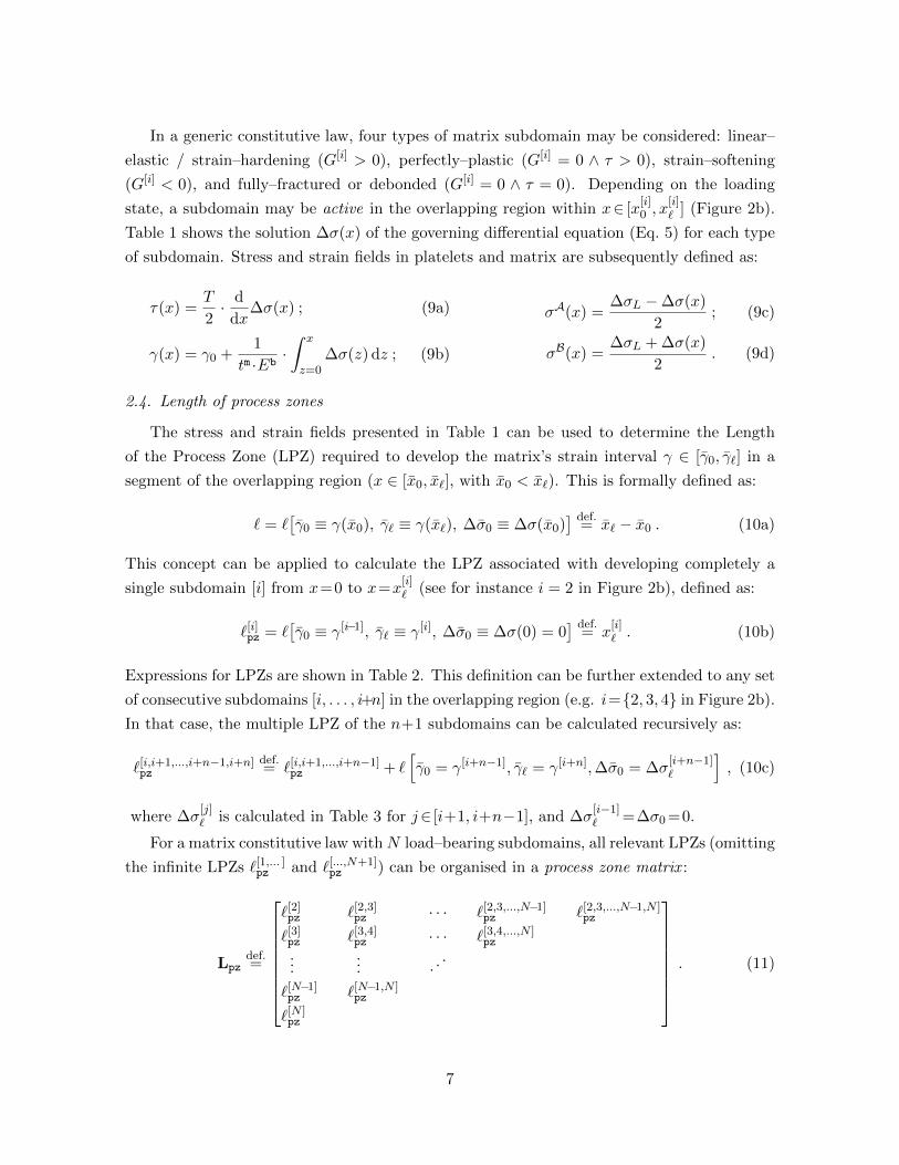
In a generic constitutive law, four types of matrix subdomain may be considered: linear–

elastic / strain–hardening (G[i] > 0), perfectly–plastic (G[i] = 0 ∧ τ > 0), strain–softening

(G[i] < 0), and fully–fractured or debonded (G[i] = 0 ∧ τ = 0). Depending on the loading

state, a subdomain may be active in the overlapping region within x∈ [x[i]0 , x

[i]` ] (Figure 2b).

Table 1 shows the solution ∆σ(x) of the governing differential equation (Eq. 5) for each type

of subdomain. Stress and strain fields in platelets and matrix are subsequently defined as:

τ(x) =T

2· d

dx∆σ(x) ; (9a)

γ(x) = γ0 +1

tm ·Eb·∫ x

z=0∆σ(z) dz ; (9b)

σA(x) =∆σL −∆σ(x)

2; (9c)

σB(x) =∆σL + ∆σ(x)

2. (9d)

2.4. Length of process zones

The stress and strain fields presented in Table 1 can be used to determine the Length

of the Process Zone (LPZ) required to develop the matrix’s strain interval γ ∈ [γ0, γ`] in a

segment of the overlapping region (x ∈ [x0, x`], with x0 < x`). This is formally defined as:

` = `[γ0 ≡ γ(x0), γ` ≡ γ(x`), ∆σ0 ≡ ∆σ(x0)

] def.= x` − x0 . (10a)

This concept can be applied to calculate the LPZ associated with developing completely a

single subdomain [i] from x=0 to x=x[i]` (see for instance i = 2 in Figure 2b), defined as:

`[i]pz = `[γ0 ≡ γ[i−1], γ` ≡ γ[i], ∆σ0 ≡ ∆σ(0) = 0

] def.= x

[i]` . (10b)

Expressions for LPZs are shown in Table 2. This definition can be further extended to any set

of consecutive subdomains [i, . . . , i+n] in the overlapping region (e.g. i={2, 3, 4} in Figure 2b).

In that case, the multiple LPZ of the n+1 subdomains can be calculated recursively as:

`[i,i+1,...,i+n−1,i+n]pz

def.= `[i,i+1,...,i+n−1]

pz + `[γ0 = γ[i+n−1], γ` = γ[i+n],∆σ0 = ∆σ

[i+n−1]`

], (10c)

where ∆σ[j]` is calculated in Table 3 for j∈ [i+1, i+n−1], and ∆σ

[i−1]` =∆σ0=0.

For a matrix constitutive law withN load–bearing subdomains, all relevant LPZs (omitting

the infinite LPZs `[1,... ]pz and `[...,N+1]pz ) can be organised in a process zone matrix :

Lpzdef.=

`[2]pz `[2,3]pz · · · `[2,3,...,N−1]pz `[2,3,...,N−1,N ]pz

`[3]pz `[3,4]pz · · · `[3,4,...,N ]pz

...... . .

.

`[N−1]pz `[N−1,N ]pz

`[N ]pz

. (11)

7

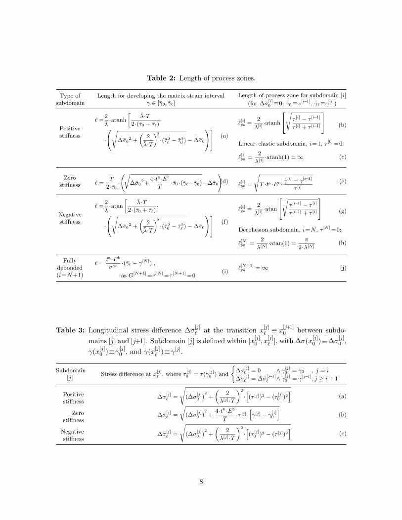
Table 2: Length of process zones.

Type ofsubdomain

Length for developing the matrix strain intervalγ ∈ [γ0, γ`]

Length of process zone for subdomain [i]

(for ∆σ[i]0 ≡0, γ0≡γ[i−1], γ`≡γ[i])

Positivestiffness

` =2

λ·atanh

[λ·T

2·(τ0 + τ`)·

·

√∆σ02 +

(2

λ·T

)2·(τ2` − τ20 )−∆σ0

(a)

`[i]pz =2

λ[i]·atanh

√τ [i] − τ [i−1]

τ [i] + τ [i−1]

(b)

Linear–elastic subdomain, i=1, τ [0] =0:

`[1]pz =2

λ[1]·atanh(1) =∞ (c)

Zerostiffness ` =

T

2·τ0·

(√∆σ0

2+4·tm ·Eb

T·τ0 ·(γ`−γ0)−∆σ0

)(d) `[i]pz =

√T ·tm ·Eb · γ

[i] − γ[i−1]

τ [i](e)

Negativestiffness

` =2

λ·atan

[λ·T

2·(τ0 + τ`)·

·

√∆σ02 +

(2

λ·T

)2·(τ20 − τ2` )−∆σ0

(f)

`[i]pz =2

λ[i]·atan

√τ [i−1] − τ [i]

τ [i−1] + τ [i]

(g)

Decohesion subdomain, i=N , τ [N ] =0:

`[N ]pz =

2

λ[N ]·atan(1) =

π

2·λ[N ](h)

Fullydebonded(i=N+1)

` =tm ·Eb

σ∞·(γ` − γ[N ]) ,

as G[N+1] =τ [N ] =τ [N+1] =0(i)

`[N+1]pz =∞ (j)

Table 3: Longitudinal stress difference ∆σ[j]` at the transition x

[j]` ≡ x

[j+1]0 between subdo-

mains [j] and [j+1]. Subdomain [j] is defined within [x[j]0 , x

[j]` ], with ∆σ(x

[j]0 )≡∆σ

[j]0 ,

γ(x[j]0 )≡γ[j]0 , and γ(x

[j]` )≡γ[j].

Subdomain[j]

Stress difference at x[j]` , where τ

[j]0 = τ(γ

[j]0 ) and

{∆σ

[j]0 = 0 ∧ γ[j]

0 = γ0 , j = i

∆σ[j]0 = ∆σ

[j−1]` ∧ γ[j]

0 = γ[j−1], j ≥ i+ 1

Positivestiffness

∆σ[j]` =

√(∆σ

[j]0 )

2+

(2

λ[j] ·T

)2

·[(τ [j])2 − (τ

[j]0 )2

](a)

Zerostiffness

∆σ[j]` =

√(∆σ

[j]0 )

2+

4·tm ·Eb

T·τ [j] ·

[γ[j] − γ[j]

0

](b)

Negativestiffness

∆σ[j]` =

√(∆σ

[j]0 )

2+

(2

λ[j] ·T

)2

·[(τ

[j]0 )2 − (τ [j])2

](c)

8

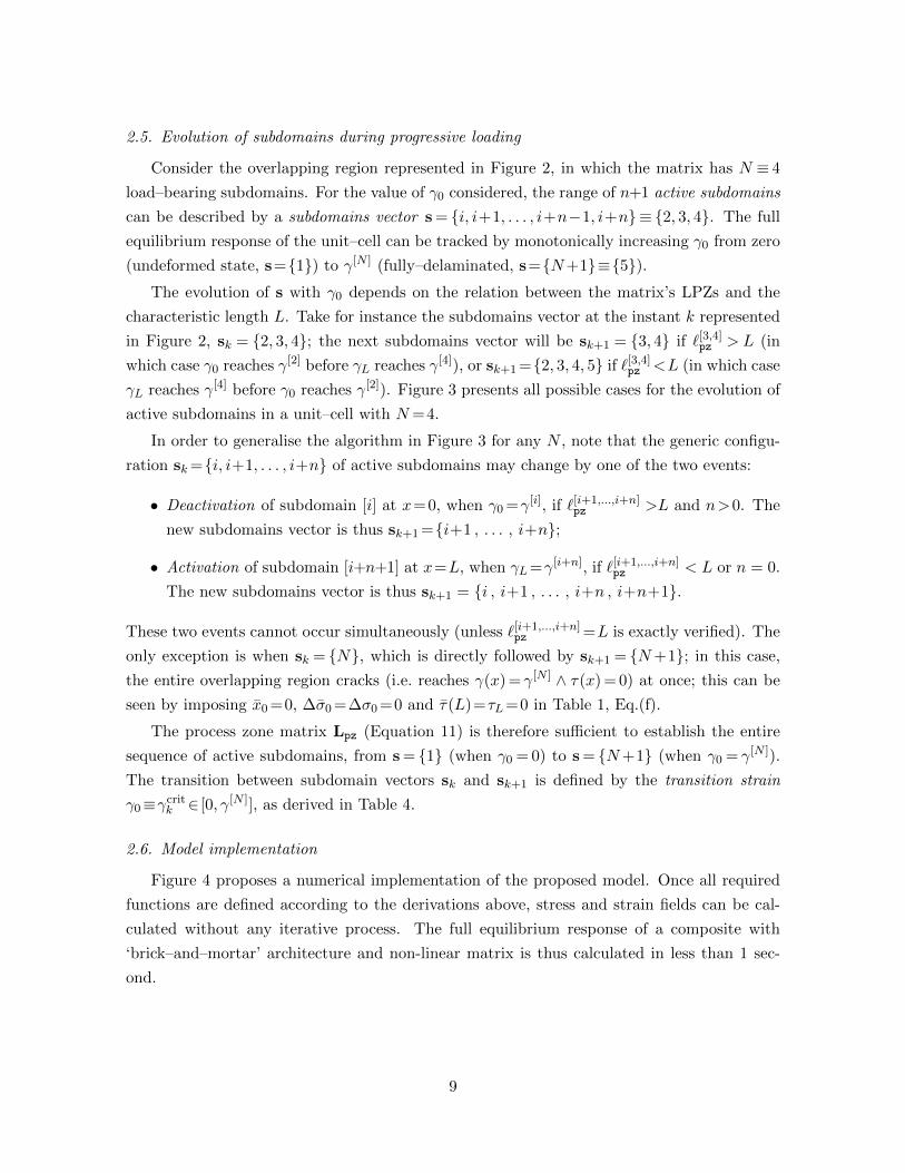
2.5. Evolution of subdomains during progressive loading

Consider the overlapping region represented in Figure 2, in which the matrix has N ≡ 4

load–bearing subdomains. For the value of γ0 considered, the range of n+1 active subdomains

can be described by a subdomains vector s= {i, i+1, . . . , i+n−1, i+n}≡ {2, 3, 4}. The full

equilibrium response of the unit–cell can be tracked by monotonically increasing γ0 from zero

(undeformed state, s={1}) to γ[N ] (fully–delaminated, s={N+1}≡{5}).The evolution of s with γ0 depends on the relation between the matrix’s LPZs and the

characteristic length L. Take for instance the subdomains vector at the instant k represented

in Figure 2, sk = {2, 3, 4}; the next subdomains vector will be sk+1 = {3, 4} if `[3,4]pz > L (in

which case γ0 reaches γ[2] before γL reaches γ[4]), or sk+1={2, 3, 4, 5} if `[3,4]pz <L (in which case

γL reaches γ[4] before γ0 reaches γ[2]). Figure 3 presents all possible cases for the evolution of

active subdomains in a unit–cell with N=4.

In order to generalise the algorithm in Figure 3 for any N , note that the generic configu-

ration sk={i, i+1, . . . , i+n} of active subdomains may change by one of the two events:

• Deactivation of subdomain [i] at x=0, when γ0 =γ[i], if `[i+1,...,i+n]pz >L and n>0. The

new subdomains vector is thus sk+1={i+1 , . . . , i+n};

• Activation of subdomain [i+n+1] at x=L, when γL=γ[i+n], if `[i+1,...,i+n]pz < L or n = 0.

The new subdomains vector is thus sk+1 = {i , i+1 , . . . , i+n , i+n+1}.

These two events cannot occur simultaneously (unless `[i+1,...,i+n]pz =L is exactly verified). The

only exception is when sk = {N}, which is directly followed by sk+1 = {N+1}; in this case,

the entire overlapping region cracks (i.e. reaches γ(x) = γ[N ] ∧ τ(x) = 0) at once; this can be

seen by imposing x0=0, ∆σ0=∆σ0=0 and τ(L)=τL=0 in Table 1, Eq.(f).

The process zone matrix Lpz (Equation 11) is therefore sufficient to establish the entire

sequence of active subdomains, from s= {1} (when γ0 = 0) to s= {N+1} (when γ0 = γ[N ]).

The transition between subdomain vectors sk and sk+1 is defined by the transition strain

γ0≡γcritk ∈ [0, γ[N ]], as derived in Table 4.

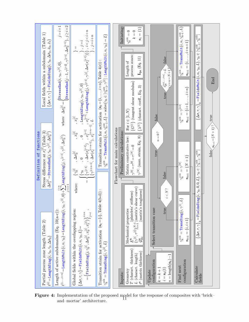
2.6. Model implementation

Figure 4 proposes a numerical implementation of the proposed model. Once all required

functions are defined according to the derivations above, stress and strain fields can be cal-

culated without any iterative process. The full equilibrium response of a composite with

‘brick–and–mortar’ architecture and non-linear matrix is thus calculated in less than 1 sec-

ond.

9

°0=°L=°[4]

°L=°[1]

`[2]pz <L; °L=°[2]

`[2;3]pz <L; °L=°[3]

`[2;3;4]pz <L; °L=°[4]

`[3;4]pz <L; °L=°[4]

`[4]pz <L; °L=°[4]

°L=°[3]

`[3]pz <L; °L=°[3]

°L=°[2]

`[2]pz >L; °0=°[1]

`[3]pz >L; °0=°[2]

`[4]pz >L; °0=°[3]

`[2;3]pz >L; °0=°[1]

`[2;3;4]pz >L; °0=°[1]

°0=°[1]

°0=°[2]

°0=°[3]

°0=°[4]

`[3;4]pz >L; °0=°[2]

Fully fractured matrix

Deactivation of subdomain [i] at x = 0

Key:

Activation of subdomain [i+n+1] at x = L

s = f1g

s = f1;2g

s = f2g s = f1;2;3g

s = f1;2;3;4gs = f2;3g

s = f3g

s = f3;4g

s = f4g

s = f2;3;4g s = f1;2;3;4;5g

s = f2;3;4;5g

s = f3;4;5g

s = f4;5g

s = f5g

Figure 3: Evolution of active subdomains during progressive loading of a composite with‘brick–and–mortar’ architecture, considering a matrix constitutive law with 4 sub-domains (followed by fracture, represented as i = N + 1 = 5).

Table 4: Transition shear strain γcritk (defined at the centre of the overlapping region,γcritk ≡γ0) between configurations sk={i, · · · , i+n} and sk+1.

Type of transition Transition strain

Deactivation: n > 0 ∧ `[i+1,...,i+n]pz >L,

sk+1 ={i+1, · · · , i+n}γ0 =γ[i] =⇒ γcrit

k = γ[i] (a)

Activation: n = 0,sk+1 ={i, i+1}

Positivestiffness:

γL =γ[i] =⇒ γcritk = γ[i]− τ [i]

|G[i]|·

(1− 1

cosh[λ[i] ·L

]) (b)

Zerostiffness:

γL =γ[i] =⇒ γcritk = γ[i]−τ [i]· L2

T ·tm ·Eb(c)

Negativestiffness:

γL =γ[i] =⇒ γcritk = γ[i]− τ [i]

|G[i]|·

(1

cos[λ[i] ·L

] − 1

)(d)

Activation: n>0 ∧ `[i]pz >L,

sk+1 ={i, · · · , i+n+1}γL =γ[i+n] =⇒ γcrit

k ∈[γcritk−1, γ

[i]] :

`[γ0 ≡ γcrit

k , : γ` ≡ γ[i+n], ∆σ0 ≡ 0]

= L

(e)

10

Definition of functions

Flo

wch

art

for

main

calc

ula

tions

Geo

met

ry

Mec

hanic

al pro

per

ties

Fin

d n

ext

configura

tion

Calc

ula

te

fiel

ds

°crit

k=

°[i+1]

s k+1

=fi

+1;:

::;i

+ng

°crit

k=

°[N

]

sk+

1=fN

+1g

`[i+1;:::;i+n]

pz

>L

_i+

n=

N+

1?

n=

0?

i<

N?

k=

k+

1

i=s k

(1)

n=

length

(sk)¡

1

s k+1=fN

+1g?

true

fals

e

true

fals

e tr

ue

fals

e

true

fals

e E

nd

¢¾[j]

0=

( EndStress¡ i;

°0;°

[i] ;

0¢ ;

j=

i+1

EndStress¡ j¡

1;°

[j¡2

] ;°[j¡1

] ;¢

¾[j¡1

]0

¢ ;j¸

i+2

Eb Gm IIc

Part

ial pro

cess

zone

length

(T

able

2)

`[i]=LengthSing¡ i;

¹°0;¹°`;¢

¹¾0

¢x[j]

`Str

ess

diffe

rence

at

(Table

3)

¢¹¾[j]

`=StressEnd¡ j;

¹°0;°

[j] ;

¢¹¾[j]

0

¢Loca

l fiel

ds

within

a s

ubdom

ain

(T

able

1)

© ¢¾;¿

;°ª =

FieldsSing¡ i;

¹°0;¢

¹¾0;¹x0;¹x`

¢

Len

gth

of act

ive

subdom

ain

s (E

q. 10(a

-c))

:

wher

e `[i;:::;i+

n]=LengthMult¡ i;

n;°

0

¢ =LengthSing¡ i;

°0;°

[i] ;

0¢ +

i+n

X

j=i+

1LengthSing¡ j;

°[j¡1

] ;°[j] ;

¢¾[j]

0

¢

Glo

bal fiel

ds

within

the

over

lappin

g r

egio

n:

wher

e:

© °[j]

0

ª=

;¢

¾[j]

0;

x[j]

0;

x[j]

`© ¢

¾;¿

;°ª =

FieldsMult¡ i;

n;°

0;L¢ =

=n F

ieldsSing¡ j;

°[j]

0;¢

¾[j]

0;x

[j]

0;x

[j]

`

¢oi+

n

j=i

;=

8 > < > :

© °0

;0

;0

;LengthSing¡ i;

°0;°

[i] ;

0¢

ª;

j=

i© °

[j¡1

];¢

¾(x

[j¡1

]

`)

;x[j¡1

]

`;

x[j¡1

]

`+LengthSing¡ j;

°[j¡1

] ;°[j] ;

¢¾(x

[j¡1

]

`)¢ª

;i<

j<

i+n

© °[i+n¡1

] ;¢

¾(x

[i+n¡1

]

`);

x[i+n¡1]

`;

Lª

;j=

i+n

Tra

nsi

tion s

train

for

act

ivation

°crit

k=TransSing¡ i;

°[i] ;

L¢

Tra

nsi

tion s

train

for

act

ivation

°crit

k=TransMult¡ i;

n;°

crit

k¡1;L¢ =

solv

e¡°02

]°crit

k¡1;°

[i] ]

:LengthMult(i

;n;°

0)=

L¢

°crit

k=TransSing¡ i;

°[i] ;

L¢

s k+1

=fi

;i+

1g

°crit

k=TransMult¡ i;

n;°

crit

k¡1;L¢

s k+1

=fi

;:::

;i+

n+

1g

© ¢¾;¿

;°ª k

=FieldsSing¡ i;

°0;0

;0;L¢ ;°

02

[°crit

k¡1;°

crit

k]

(pla

tele

ts'st

i®nes

s)

(matr

ix's

shea

rcu

rve)

(matr

ix's

toughnes

s)

T(c

hara

ct.

thic

knes

s)

L(c

hara

ct.

length

)

tm(m

atr

ixth

icknes

s)

© ¢¾;¿

;°ª k

=FieldsMult¡ i;

n;°

0;L¢ ;°

02

[°crit

k¡1;°

crit

k]

f°[i] ;

¿[i] gN¡1

i=1

Inputs

:

°crit

0=

0

k=

0

s1

=f1g

Initia

ting:

Update

co

nfigura

tion

Sel

ect

transi

tion c

ase

¢¾[j]

0=

( StressEnd¡ i;

°0;°

[i] ;

0¢ ;

j=

i+1

StressEnd¡ j¡

1;°

[j¡2

] ;°[j¡1

] ;¢

¾[j¡1

]0

¢ ;j¸

i+2

(sk=fig;

Table

4(b

-d))

:(s

k=fi

;:::

;i+

ng;

Table

4(e

)):

Matr

ix c

onst

itutive

law

:

°[0]=

¿[0]=

¿[N

]=

0

°[N

](m

ax.st

rain

,Eq.8)

Pre

lim

inary

calc

ula

tions:

For

i2

[1;N

]:© G

[i]ª

(tangen

tsh

ear

modulu

s)© ¸

[i]ª

(chara

ct.co

e®.,

Eq.3)

Len

gth

of

pro

cess

zones

:

Lpz

(Eq.11

)

x[j]

`

Figure 4: Implementation of the proposed model for the response of composites with ‘brick–and–mortar’ architecture.

11

3. Results

3.1. Analysis of model predictions

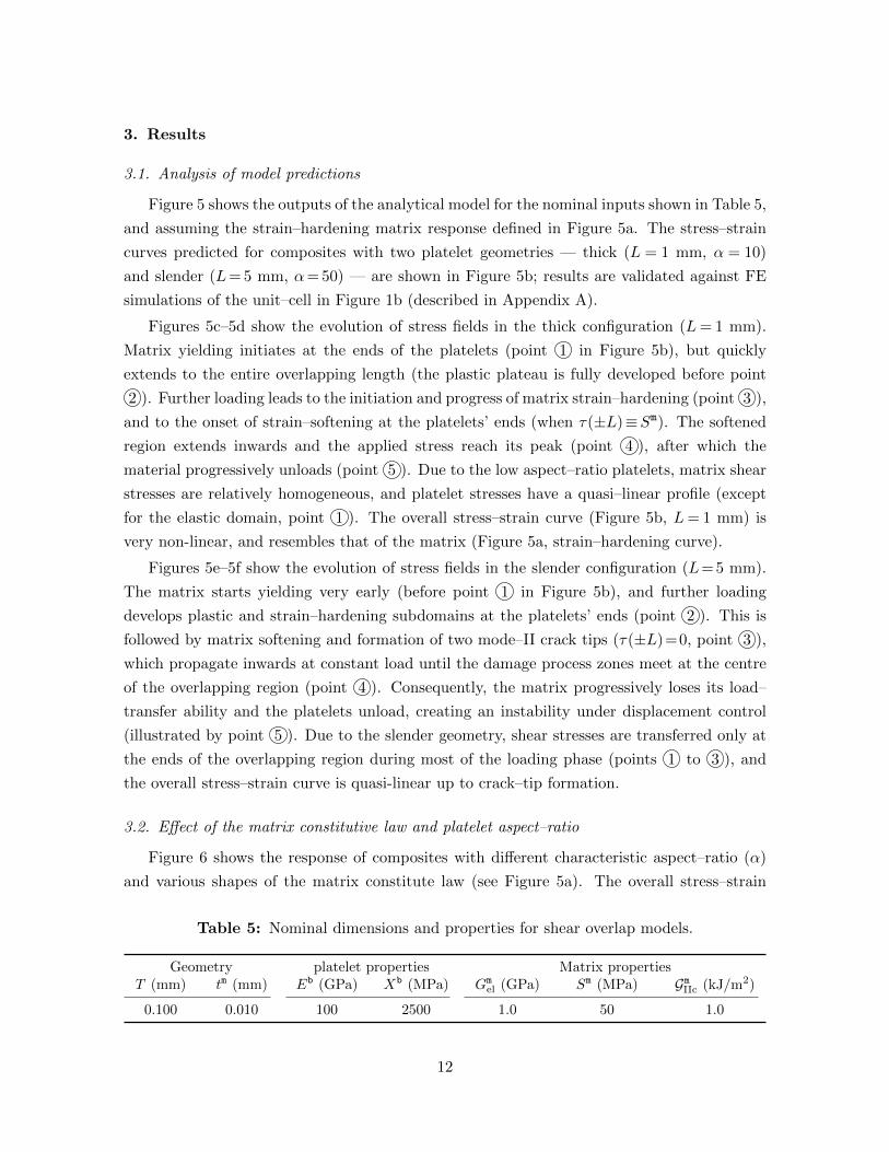
Figure 5 shows the outputs of the analytical model for the nominal inputs shown in Table 5,

and assuming the strain–hardening matrix response defined in Figure 5a. The stress–strain

curves predicted for composites with two platelet geometries — thick (L = 1 mm, α = 10)

and slender (L= 5 mm, α= 50) — are shown in Figure 5b; results are validated against FE

simulations of the unit–cell in Figure 1b (described in Appendix A).

Figures 5c–5d show the evolution of stress fields in the thick configuration (L= 1 mm).

Matrix yielding initiates at the ends of the platelets (point 1 in Figure 5b), but quickly

extends to the entire overlapping length (the plastic plateau is fully developed before point

2 ). Further loading leads to the initiation and progress of matrix strain–hardening (point 3 ),

and to the onset of strain–softening at the platelets’ ends (when τ(±L)≡Sm). The softened

region extends inwards and the applied stress reach its peak (point 4 ), after which the

material progressively unloads (point 5 ). Due to the low aspect–ratio platelets, matrix shear

stresses are relatively homogeneous, and platelet stresses have a quasi–linear profile (except

for the elastic domain, point 1 ). The overall stress–strain curve (Figure 5b, L= 1 mm) is

very non-linear, and resembles that of the matrix (Figure 5a, strain–hardening curve).

Figures 5e–5f show the evolution of stress fields in the slender configuration (L=5 mm).

The matrix starts yielding very early (before point 1 in Figure 5b), and further loading

develops plastic and strain–hardening subdomains at the platelets’ ends (point 2 ). This is

followed by matrix softening and formation of two mode–II crack tips (τ(±L)=0, point 3 ),

which propagate inwards at constant load until the damage process zones meet at the centre

of the overlapping region (point 4 ). Consequently, the matrix progressively loses its load–

transfer ability and the platelets unload, creating an instability under displacement control

(illustrated by point 5 ). Due to the slender geometry, shear stresses are transferred only at

the ends of the overlapping region during most of the loading phase (points 1 to 3 ), and

the overall stress–strain curve is quasi-linear up to crack–tip formation.

3.2. Effect of the matrix constitutive law and platelet aspect–ratio

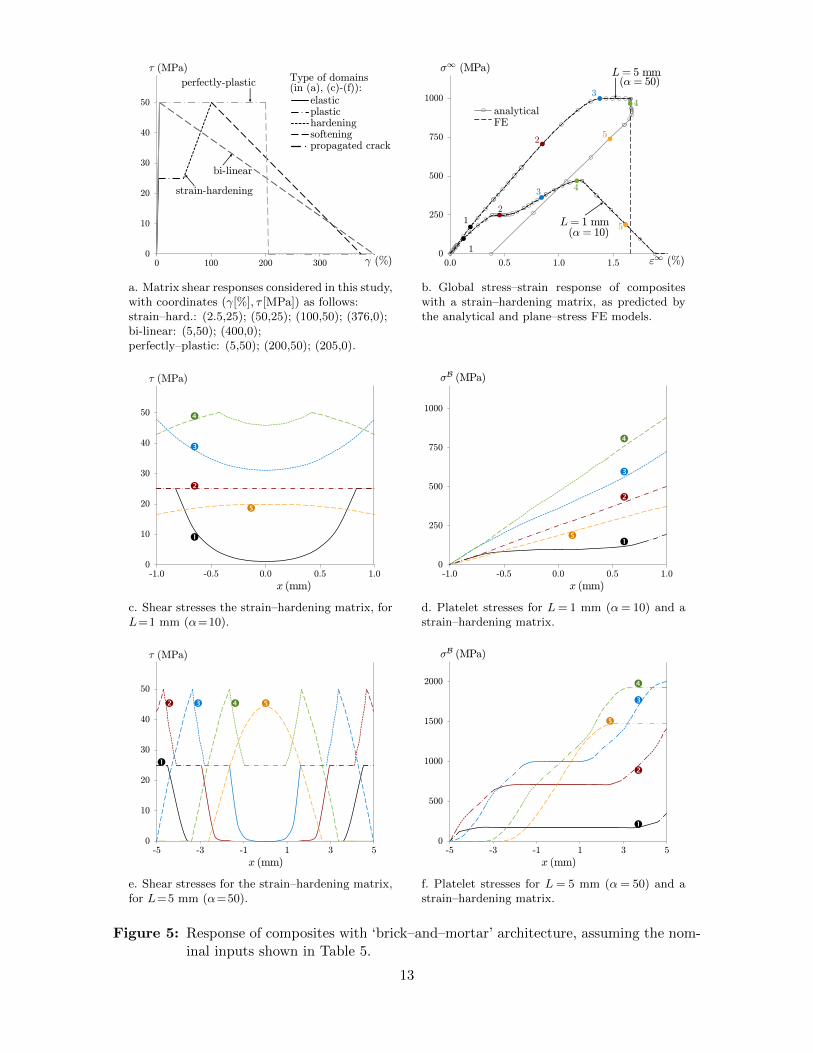
Figure 6 shows the response of composites with different characteristic aspect–ratio (α)

and various shapes of the matrix constitute law (see Figure 5a). The overall stress–strain

Table 5: Nominal dimensions and properties for shear overlap models.

Geometry platelet properties Matrix propertiesT (mm) tm (mm) Eb (GPa) Xb (MPa) Gm

el (GPa) Sm (MPa) GmIIc (kJ/m2)

0.100 0.010 100 2500 1.0 50 1.0

12

0

10

20

30

40

50

0 100 200 300

¿ (MPa)

° (%)

perfectly-plastic

bi-linear

strain-hardening

Type of domains (in (a), (c)-(f)):

elasticplastichardeningsofteningpropagated crack

a. Matrix shear responses considered in this study,with coordinates (γ[%], τ [MPa]) as follows:strain–hard.: (2.5,25); (50,25); (100,50); (376,0);bi-linear: (5,50); (400,0);perfectly–plastic: (5,50); (200,50); (205,0).

0

250

500

750

1000

0.0 0.5 1.0 1.5

analytical FE

1

1

2

2

3 4

5

3 4

5

¾1 (MPa)

"1 (%)

(® = 50)L= 5 mm

(® = 10)L= 1 mm

b. Global stress–strain response of compositeswith a strain–hardening matrix, as predicted bythe analytical and plane–stress FE models.

0

10

20

30

40

50

-1.0 -0.5 0.0 0.5 1.0

¿ (MPa)

x (mm)

c. Shear stresses the strain–hardening matrix, forL=1 mm (α=10).

0

250

500

750

1000

-1.0 -0.5 0.0 0.5 1.0

¾B (MPa)

x (mm)

d. Platelet stresses for L= 1 mm (α= 10) and astrain–hardening matrix.

0

10

20

30

40

50

-5 -3 -1 1 3 5

¿ (MPa)

x (mm)

e. Shear stresses for the strain–hardening matrix,for L=5 mm (α=50).

0

500

1000

1500

2000

-5 -3 -1 1 3 5

¾B (MPa)

x (mm)

f. Platelet stresses for L= 5 mm (α= 50) and astrain–hardening matrix.

Figure 5: Response of composites with ‘brick–and–mortar’ architecture, assuming the nom-inal inputs shown in Table 5.

13

curve of low aspect–ratio configurations resembles the matrix constitutive law (e.g. compare

the curves for α=5 in Figures 6a–6c with those in Figure 5a); however, as the characteristic

aspect–ratio increases, the composite’s response becomes quasi-linear and almost independent

of the matrix type (e.g. curves for α=100 in Figures 6a–6c).

For relatively thick configurations (α . 10), the strength of the composite increases with

the characteristic aspect–ratio, in agreement with a yield criterion (Equation 1, see Figure 6d).

For slender configurations (α & 30), on the contrary, the model predicts that the composite’s

strength becomes independent of aspect ratio and converges to a fracture criterion (Equa-

tion 2). The matrix response affects the transition between these two domains.

0

250

500

750

1000

0.0 0.5 1.0 1.5 2.0 2.5

onset of non-linearity

onset ofsoftening

fully formedcrack tip

¾1 (MPa)

"1 (%)

®= 5

®= 100

50

25

10

Key for symbols in (a)-(c):

a. Overall stress–strain response of compositeswith a strain–hardening matrix.

0

250

500

750

1000

0.0 0.5 1.0 1.5 2.0 2.5

¾1 (MPa)

"1 (%)

®= 5

®= 100

50

25

10

b. Overall stress–strain response of compositeswith a bi-linear matrix.

0

250

500

750

1000

0.0 0.5 1.0 1.5 2.0 2.5

¾1 (MPa)

"1 (%)

®= 5

®= 10050

25

10

c. Overall stress–strain response of compositeswith a perfectly–plastic matrix.

0

250

500

750

1000

0 10 20 30 40

perfectly-plastic

bi-linear

strain-hardening

strength criterion (Eq. 1)

toughness criterion (Eq. 2)

Matrix constitutive law:

X1 (MPa)

®

(L±T )

d. Effect of the characteristic aspect–ratio α onthe composite’s strength.

Figure 6: Effect of characteristic aspect–ratio α and matrix constitutive law on the responseof composites with ‘brick–and–mortar’ architecture. Matrix responses are shownin Figure 5a, and all other properties are defined in Table 5.

14

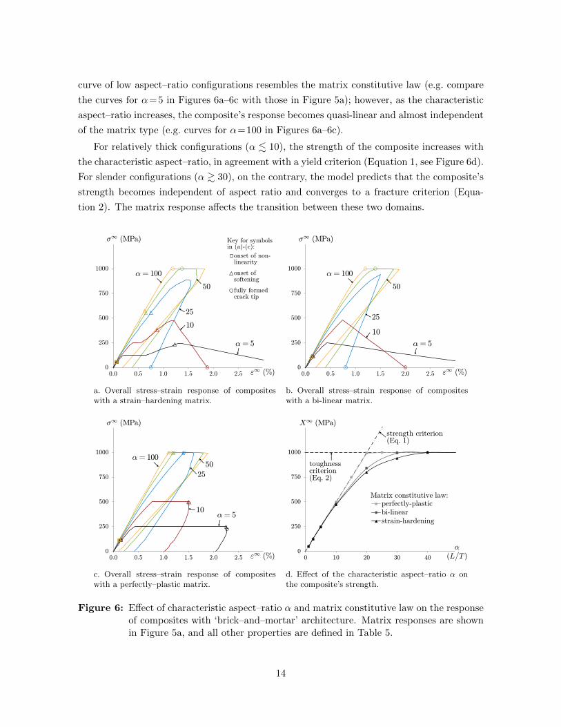
3.3. Effect of the thickness and volume content of the platelet and matrix phases

The effect of varying the thickness and content of platelet and matrix phases on the

response of composites is explored in Figure 7. A thicker matrix makes the composite more

ductile if the platelets are thick and the matrix strain–hardens (α = 10 in Figure 7a), but

not if the platelets are slender (α= 100 in Figure 7a) or the matrix is bi-linear (Figure 7b).

The initial Young’s modulus (E∞) is slightly reduced by increasing the matrix thickness

(Figure 7e), and the overall strength remains virtually unaffected (Figure 7f). Note that

composite stresses are based on the cross section of the platelets (see Equation 7).

Using thinner platelets delays final failure and increases the strength of composites with

slender configurations (see α & 25 in Figures 7c, 7d and 7f), and increases the ductility of

composites with thicker configurations and strain–hardening matrix (see α=10 in Figure 7c).

3.4. Effect of matrix toughness and geometric scaling

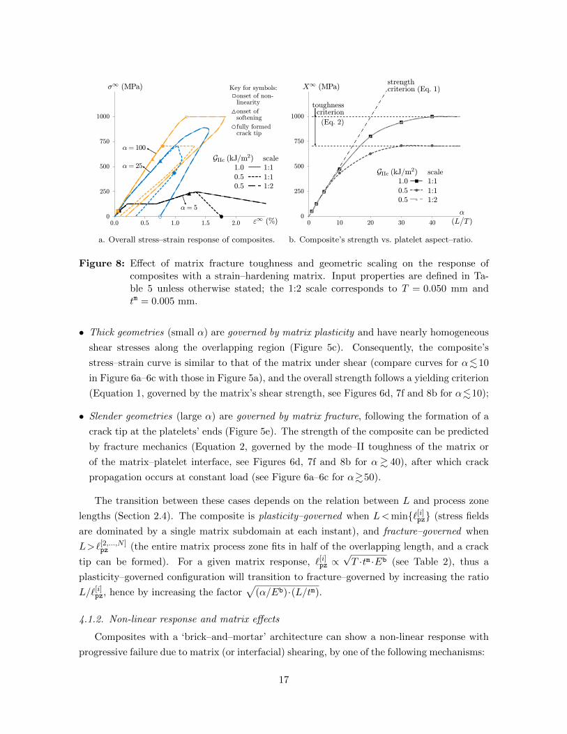
Figure 8 shows that reducing the fracture toughness GmIIc has no influence on the loading

response of composites with thick platelets (see coincident rising curves for α=5 in Figure 8a).

However, slender configurations undergo premature crack initiation if the matrix is less tough;

this can be seen in in Figures 8a–8b, by comparing the two sets of curves with distinct matrix

toughnesses (GmIIc = 1.0 kJ/m2 and GmIIc = 0.5 kJ/m2) and nominal 2D geometry (with T and

tm defined in Table 5, identified by the ‘1:1 scale’ label) when α&25.

The effect of reducing GmIIc can be counter–balanced by proportionally scaling down the 2D

geometry of the composite (i.e. by reducing T , tm and L by the same factor). This is illustrated

in Figure 8, which shows two sets of perfectly coincident stress–strain curves: the first set

(labelled as ‘GmIIc = 1.0 kJ/m2, 1:1 scale’) considers the nominal toughness and geometry (i.e.

with T , tm and GmIIc as in Table 5) and the aspect–ratios shown, while the second set (labelled

as ‘GmIIc = 0.5 kJ/m2, 1:2 scale’) considers halved nominal values for T , tm and GmIIc, and the

same aspect–ratios. Figure 8 considers a strain–hardening matrix, but similar effects were

observed for a wide range of different matrix constitutive laws.

4. Discussion

4.1. Mechanical response of composites with ‘brick–and–mortar’ architecture

4.1.1. Effect of geometric configuration

Composites with a ‘brick–and–mortar’ architecture can present a wide range of mechanical

responses, which depend largely on the characteristic aspect–ratio α=L/T . Assuming that

the platelets withstand the applied stresses, two types of configuration were identified in

Section 3:

15

0

250

500

750

1000

0.0 0.5 1.0 1.5 2.0

¾1 (MPa)

"1 (%)

tm (mm)

100

25

10

®

0.010 0.020

Key for lines in (a)-(b):

a. Response of composites with a strain–hardening matrix of different thicknesses.

0

250

500

750

1000

0.0 0.5 1.0 1.5 2.0

onset of non-linearity

onset ofsoftening

fully formedcrack tip

¾1 (MPa)

"1 (%)

Key for symbols in (a)-(d):

b. Response of composites with a bi-linear matrixof different thicknesses.

0

250

500

750

1000

1250

0.0 0.5 1.0 1.5 2.0 2.5

¾1 (MPa)

"1 (%)

T (mm)

100

25

10

®

0.100 0.050

Key for lines in (c)-(d):

c. Response of composites with different plateletthicknesses and a strain–hardening matrix.

0

250

500

750

1000

1250

0.0 0.5 1.0 1.5 2.0 2.5

¾1 (MPa)

"1 (%)

d. Response of composites with different plateletthicknesses and a bi-linear matrix.

0

25

50

75

100

0 10 20 30 40 50

E1 (GPa)

T; tm (mm)

0.100, 0.010 (nominal)

0.050, 0.010 (thinner platelets)

0.100, 0.020 (thicker matrix)

91

83

83

V b (%)

Eb

®

(L±T )

e. Initial stiffness of composites vs. characteris-tic aspect ratio, for different platelet and matrixthicknesses and a strain–hardening matrix.

0

250

500

750

1000

1250

0 10 20 30 40 50

X1 (MPa)

T=0:100 mm

®

(L±T )

strength criterion (Eq. 1)

toughness criterion (Eq. 2)

T; tm (mm)

0.100, 0.010 (nominal)

0.050, 0.010 (thinner platelets)

0.100, 0.020 (thicker matrix)

91

83

83

V b (%)

f. Strength of composites vs. characteristic aspectratio, for different platelet and matrix thicknessesand a strain–hardening matrix.

Figure 7: Effect of the thickness and content of the platelets and matrix on the responseof composites. Matrix responses are shown in Figure 5a, and other propertiesare defined in Table 5 unless stated otherwise. Note that composite stresses arecalculated neglecting the matrix thickness (see Equation 7).

16

onset of non-linearity

onset ofsoftening

fully formedcrack tip

0

250

500

750

1000

0.0 0.5 1.0 1.5 2.0

¾1 (MPa)

"1 (%)

®= 100

®= 25

®= 5

1:1

1:1

1:2

1.0

0.5

0.5

GIIc (kJ=m2) scale

Key for symbols:

a. Overall stress–strain response of composites.

0

250

500

750

1000

0 10 20 30 40

X1 (MPa)strength criterion (Eq. 1)

toughness criterion

(Eq. 2)

1:1

1:1

1:2

1.0

0.5

0.5

GIIc (kJ=m2) scale

®

(L±T )

b. Composite’s strength vs. platelet aspect–ratio.

Figure 8: Effect of matrix fracture toughness and geometric scaling on the response ofcomposites with a strain–hardening matrix. Input properties are defined in Ta-ble 5 unless otherwise stated; the 1:2 scale corresponds to T = 0.050 mm andtm = 0.005 mm.

• Thick geometries (small α) are governed by matrix plasticity and have nearly homogeneous

shear stresses along the overlapping region (Figure 5c). Consequently, the composite’s

stress–strain curve is similar to that of the matrix under shear (compare curves for α.10

in Figure 6a–6c with those in Figure 5a), and the overall strength follows a yielding criterion

(Equation 1, governed by the matrix’s shear strength, see Figures 6d, 7f and 8b for α.10);

• Slender geometries (large α) are governed by matrix fracture, following the formation of a

crack tip at the platelets’ ends (Figure 5e). The strength of the composite can be predicted

by fracture mechanics (Equation 2, governed by the mode–II toughness of the matrix or

of the matrix–platelet interface, see Figures 6d, 7f and 8b for α & 40), after which crack

propagation occurs at constant load (see Figure 6a–6c for α&50).

The transition between these cases depends on the relation between L and process zone

lengths (Section 2.4). The composite is plasticity–governed when L<min{`[i]pz} (stress fields

are dominated by a single matrix subdomain at each instant), and fracture–governed when

L>`[2,...,N ]pz (the entire matrix process zone fits in half of the overlapping length, and a crack

tip can be formed). For a given matrix response, `[i]pz ∝√T ·tm ·Eb (see Table 2), thus a

plasticity–governed configuration will transition to fracture–governed by increasing the ratio

L/`[i]pz, hence by increasing the factor√

(α/Eb)·(L/tm).

4.1.2. Non-linear response and matrix effects

Composites with a ‘brick–and–mortar’ architecture can show a non-linear response with

progressive failure due to matrix (or interfacial) shearing, by one of the following mechanisms:

17

(i) Non-linear matrix response, effective in thick configurations when the matrix presents

significant plasticity and strain hardening before softening (see α . 10 in Figures 6a

and 6c). The composite becomes more ductile if the matrix content increases (i.e. when

tm increases or T decreases, see Figures 7a and 7c), or if the matrix’s failure strain

increases (as the composite’s stress–strain curve reproduces that of the matrix for small

α, compare Figures 7a–7c with Figure 5a);

(ii) Progressive crack formation in the matrix (or matrix–platelet interface), which occurs

in slender configurations with L≈`[2,...,N ]pz (see α={25, 50} in Figures 5–6). In this case,

a damage process zone develops along a great part of the overlapping length, resulting

in progressive loss of stiffness due to matrix softening. This mechanism is enhanced by

thinner platelets or a tougher matrix (see α & 25 in Figures 7c–7d and 8a), and it is

mostly independent of the matrix thickness and constitutive law (see Figures 7a–7b).

4.1.3. Macroscopic response

Figures 5 to 8 show the response of a single composite unit–cell, as seen in Figure 1b. To

understand the macroscopic response of the composite, consider now a chain of n identical

unit–cells in series. Along the loading phase (with positive tangent stiffness), σ∞M ≡ σ∞uc and

ε∞M ≡ ε∞uc (where M and uc represent respectively the macroscopic and unit–cell responses).

However, due to intrinsic material variability, one weaker cell will reach its strength X∞ (and

associated failure strain e∞) first, after which deformation will localise. Consequently, the

weakest cell will follow its equilibrium softening response, while the remaining cells will unload

elastically (subscript un in Equation 12a), leading to the macroscopic unloading response

calculated in Equation 12b:{σ∞un ≡ σ∞ucε∞un = e∞uc −

(X∞ − σ∞un

)/E∞

, (12a)

{σ∞M ≡ σ∞ucε∞M =

[ε∞uc + (n− 1)·ε∞un

]/n. (12b)

Figure 9 compares the response of a unit–cell (n=1) to that of a finite composite volume

(finite n) or of an infinitely large (n→∞) sample. This shows that:

a. All non-linearities developed in the unit–cell before the strength is reached are reproduced

in the macroscopic response. Thick configurations with a strain–hardening matrix dissipate

a significant amount of energy through diffuse plasticity and damage (Figure 9a);

b. Stress plateaus at σ∞≈X∞ are not replicated in the macroscopic response, as softening

starts just below the plateau level of the n−1 infinitesimally stronger cells; permanent strains

and energy dissipation through plasticity or damage are therefore negligible (Figure 9b).

18

0

100

200

300

400

500

0.0 0.5 1.0 1.5 2.0

¾1 (MPa)

"1 (%)

n= 1 (unit-cell)

2

5

10

(elastic unloading) n!1

M

a. Unit–cell with strain–hardening (α=10).

0

250

500

750

1000

0.0 0.5 1.0 1.5 2.0

¾1 (MPa)

"1 (%)

n= 1 (unit-cell)

2 5

10

(elastic unloading) n!1

M

b. Unit–cell with stress plateau (α=100).

Figure 9: Macroscopic stress–strain response of composites with ‘brick–and–mortar’ archi-tecture with n unit–cells in series. Both cases consider the nominal geometry andproperties (Table 5), and a strain–hardening matrix.

c. The unloading response is governed by the overall size of a structure [14]. Even a material

with stable progressive failure at the small scale will fail unstably if loaded in a sufficiently

large structure (compare n=1 with n→∞ in Figure 9a).

4.2. Optimal configuration for brittle matrix systems

Figure 9b shows that, as soon as a crack tip forms in the matrix, it propagates at constant

load leading to damage localisation — which limits ductility and energy absorption. Conse-

quently, progressive crack formation in the matrix (see Section 4.1.2) generates macroscopic

non-linearities only before a crack tip is formed (i.e. before reaching the stress plateau).

Because this mechanism operates in toughness–governed configurations (see Figure 6d),

in order to fully utilise the tensile strength of the platelets one must impose that:

X∞G = Xb/

2 (where X∞G is given from Eq. 2), hence T ? = 4·Eb ·GmIIc/

(Xb)2 . (13)

This defines the optimal characteristic thickness: if T < T ? the platelets fail under tension

before the matrix fractures, and vice–versa (see Figure 10a).

The effect of progressive matrix fracture is fairly independent of the matrix thickness and

constitutive law (see Figures 7a–7b), hence a thin bi-linear matrix (N = 2) is considered for

simplicity. According to Figure 6b and Section 4.1.1, a crack tip can fully form in configura-

tions with L≥`[2,...,N ]pz , but the non-linearity before the stress plateau decreases as L increases

further. The optimal characteristic length is therefore defined in this case as:

19

0

500

1000

1500

0.000 0.050 0.100 0.150

X1 (MPa)

T (mm)

X1 =Xb

2

X1 =X1G

T = T?

matrix shear fracture

platelet tensile failure

(Eq. 13)

(Eq. 2)

a. Strength of slender configurations anddefinition of the optimal thickness T ?.

0

500

1000

1500

0.0 1.0 2.0 3.0

loading curve up to failure

matrix shear fracture

platelet tensile failure

matrix shear yielding

theoretical shear-lag response

¾1 (MPa)

"1 (%)

T = T?; ® = ®?

T = T?; ® = 1:5¢®?

T = T?; ® = 0:5¢®?T = 1:5¢T?; ® = ®?

T = 0:5¢T?; ® = ®? (optimal configuration)

b. Response of the optimised configuration for matrixfracture (see Equations 13 and 14c) and its variations.

Figure 10: Response of composites with ‘brick–and–mortar’ architecture with slender config-urations and a bi-linear matrix response. For the nominal properties in Table 5,T ?=0.064 mm, L?=2.513 mm and α?=39.3).

L? = `[N≡2]pz , which following Eq.(h) in Table 2 leads to L? =π

2·

√T ·tm ·Eb

2·|G[N≡2]|. (14a)

For a thin, brittle bi-linear matrix phase with maximum shear strength Sm,

γ[N ] (Eq.8)=2·GmIIcSm ·tm

and γ[N ]−γ[1]≈γ[N ] , hence G[N ] =Sm

γ[N ]−γ[1]≈ (Sm)2 ·tm

2·GmIIc; (14b)

replacing in Equation 14a,

L? ≈ π

2·Sm·√

2·T ·Eb ·GmIIc . (14c)

A composite with optimal dimensions T ? and L? will therefore fail at:

σ∞ = X∞G =Xb

2and ε∞ = e∞ =

tm · γ[N ]

2 · L?+

Xb

2 · Eb(following Equation 7). (15a)

Replacing γ[N ] and L? according to Equations 14b–14c, and then defining T =T ? from Equa-

tion 13 yields:

e∞ =2

π·√GmIIcT ·Eb

+Xb

2 · Eb=⇒ e∞ =

(1

π+

1

2

)·X

b

Eb. (15b)

Figure 10b presents the response of a composite with ‘brick–and–mortar’ geometry opti-

mised for matrix fracture (defined by T ? and α? =L?/T ?, following Equations 13 and 14c).

20

While this mechanism leads to non-linearity and progressive failure, it has limited poten-

tial for ductility (as the optimal configuration with thin bi-linear matrix will fail at a strain

e∞≈82%·eb, where eb is the failure strain of the linear–elastic platelets, see Equation 15b).

Modifying the optimal geometry results in further loss of strength and/or failure strain.

4.3. Analysis of the proposed model in the scope of the literature

The analytical model for composites with ‘brick–and–mortar’ architecture presented in

this paper complements existing literature with the following features:

a. This model bridges the two most widely used theories for sub-critical discontinuous compos-

ites: (i) yield–slip theory (governed by the shear strength of the matrix) [5] and (ii) fracture

mechanics (governed by the mode–II toughness of the matrix or interface) [6, 7]. While

there is significant debate in the literature [8–13] on which criterion should be used for

different types of matrix, Figure 6d shows that they are both accurate for most matrices,

but limited in the range of applicable geometries of the platelets or inclusions;

b. The model predicts non-linear size effects on the strength of composites with ‘brick–and–

mortar’ architecture, tending to plasticity theory for thick (small α) platelets, and to

fracture mechanics for slender (large α) platelets. The characteristic length of the damage

process zone (calculated in Equation 10 and Table 2) defines the transition between the

two asymptotic responses, which agrees with Bazant’s size–effect law [14];

c. This is the first analytical model in the literature to consider a generic non-linear response

(as long as it is piecewise linear) for the soft phase, thus providing a flexible tool for

investigating the effect of different matrices on the response of discontinuous composites;

d. Due to its analytical formulation, this model calculates the full response and local fields in

less than 1 second, while considering a completely non-linear matrix response. The model

is thus particularly suitable for parametric studies and Monte-Carlo analyses.

e. The model can be extended to staggered discontinuous composites with other types of

inclusions (by having T = Ab/Cb, where Ab is the area and Cb is the perimeter of the

inclusions’ cross–section), or to composites with randomly shifted platelet–ends, platelets

with stochastic strength or complex load sharing laws [16, 17]. These developments will

be the scope of further publications.

5. Conclusions

An analytical model for the tensile response of perfectly staggered discontinuous compos-

ites was developed. The model is based on shear–lag, and considers a generic piecewise linear

21

matrix constitutive law (including non-linearity and fracture). Process zone lengths are cal-

culated and used in an efficient implementation framework, thus the full equilibrium response

of composites with ‘brick–and–mortar’ architecture is determined almost instantaneously.

Parametric studies showed that the response of composites with thick platelets are dom-

inated by plasticity, while those with slender platelets are governed by fracture mechanics.

This leads to non-linear size effects influenced by the length of the matrix’s damage process

zone.

Results suggest that well-designed discontinuous composites can present progressive fail-

ure, energy dissipation and enhanced failure strains, achieved by two different mechanisms:

plasticity and strain–hardening of the matrix (leading to ductile composites with modest

strength), and fracture of the matrix (leading to strong composites with non-linear response).

This concept is experimentally demonstrated in a subsequent paper [18].

Acknowledgements

This work was funded under the EPSRC Programme Grant EP/I02946X/1 on High Per-

formance Ductile Composite Technology, in collaboration with the University of Bristol.

Appendix A. Finite Element validation of the proposed analytical model

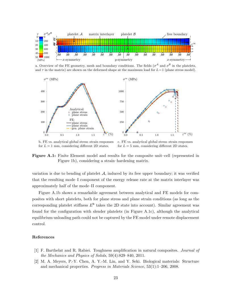
The analytical model was validated by 2D FE analyses illustrated in Figure A.1, with nom-

inal dimensions and properties defined in Table 5. The platelets were modelled as an isotropic

linear–elastic material with Young’s modulus Eb and Poisson’s ratio νf = 0.3. The matrix

was modelled as an isotropic material with initial linear–elastic behaviour (with Young’s mod-

ulus Em = 2 ·Gm ·(1 + νm) and matrix Poisson’s ratio νm = 0.5); its non-linear response was

modelled by von Mises plasticity, where the von Mises equivalent stresses (σ[i]vM) and strains

(ε[i]vM) were calculated from the stress–strain curve of a strain–hardening matrix under shear

(see Figure 5a) as:

σ[i]vM =

√3 · τ [i] and ε

[i]vM =

√3

3· γ[i] . (A.1)

Two characteristic lengths (L = 1.0 mm and L = 5.0 mm) were considered. The mod-

els were discretised using 4–nodes elements with full integration; one element was used to

represent the matrix’s through–the–thickness direction, and five elements for the platelets.

The models were run under displacement control using Abaqus Standard [19] implicit solver,

assuming plane stress, plane strain or generalised plane strain.

The deformed shape of the composite unit–cell with thick platelets is represented in Fig-

ure A.1a, where the fields represent the longitudinal stresses in the platelets and shear stresses

in the matrix. It is confirmed that platelet stresses are generally uniform across their thick-

ness, with the largest through–the–thickness variation found near the end of platelet A. This

22

"1

platelet A platelet B matrix interlayer 0

200

400

600

800

1000

0

10

20

30

40

50

¾A;¾B

(MPa)

¿

y-symmetry x-symmetry x-symmetry

free boundary

a. Overview of the FE geometry, mesh and boundary conditions. The fields (σA and σB in the platelets,and τ in the matrix) are shown on the deformed shape at the maximum load for L=1 (plane stress model).

0

100

200

300

400

0.0 0.5 1.0 1.5

plane stressplane strain

plane stressplane straingen. plane strain

¾1 (MPa)

"1 (%)

Analytical:

FE:

b. FE vs. analytical global stress–strain responsesfor L = 1 mm, considering different 2D states.

0

250

500

750

1000

0.0 0.5 1.0 1.5

¾1 (MPa)

"1 (%)

c. FE vs. analytical global stress–strain responsesfor L = 5 mm, considering different 2D states.

Figure A.1: Finite Element model and results for the composite unit–cell (represented inFigure 1b), considering a strain–hardening matrix.

variation is due to bending of platelet A, induced by its free upper boundary; it was verified

that the resulting mode–I component of the energy release rate at the matrix interlayer was

approximately half of the mode–II component.

Figure A.1b shows a remarkable agreement between analytical and FE models for com-

posites with short platelets, both for plane stress and plane strain conditions (as long as the

corresponding platelet stiffness Eb takes the 2D state into account). Similar agreement was

found for the configuration with slender platelets (in Figure A.1c), although the analytical

equilibrium unloading path could not be captured by the FE model under remote displacement

control.

References

[1] F. Barthelat and R. Rabiei. Toughness amplification in natural composites. Journal ofthe Mechanics and Physics of Solids, 59(4):829–840, 2011.

[2] M. A. Meyers, P.-Y. Chen, A. Y.-M. Lin, and Y. Seki. Biological materials: Structureand mechanical properties. Progress in Materials Science, 53(1):1–206, 2008.

23

[3] F. Barthelat, A. K. Dastjerdi, and R. Rabiei. An improved failure criterion for biologicaland engineered staggered composites. Journal of the Royal Society Interface, 10(79),2013.

[4] M. R. Begley, N. R. Philips, B. G. Compton, D. V. Wilbrink, R. O. Ritchie, and M. Utz.Micromechanical models to guide the development of synthetic ’brick and mortar’ com-posites. Journal of the Mechanics and Physics of Solids, 60(8):1545–1560, 2012.

[5] A. Kelly and W. R. Tyson. Tensile properties of fibre–reinforced metals: Copper/tungstenand copper/molybdenum. Journal of the Mechanics and Physics of Solids, 13(6):329–338,1965.

[6] J. O. Outwater and M. C. Murphy. Fracture energy of unidirectional laminates. ModernPlastics, 47(September issue):160–168, 1970.

[7] Y.-C. Gao, Y.-W. Mai, and B. Cotterell. Fracture of fiber–reinforced materials. Journalof Applied Mathematics and Physics, 39(4):550–572, 1988.

[8] H. Stang, Z. Li, and S. P. Shah. Pullout problem — stress versus fracture mechanicalapproach. Journal of Engineering Mechanics, 116(10):2136–2150, 1990.

[9] C. K. Y. Leung. Fracture–based two–way debonding model for discontinuous fibres inelastic matrix. Journal of Engineering Mechanics, 118(11):2298–2318, 1992.

[10] M. R. Piggott, M. Ko, and H. Y. Chuang. Aligned short-fibre-reinforced thermosets —experiments and analysis lend little support for established theory. Composites Scienceand Technology, 48(1-4):291–299, 1993.

[11] J. A. Nairn. On the use of shear–lag methods for analysis of stress transfer in unidirec-tional composites. Mechanics of Materials, 26(2):63–80, 1997.

[12] S. Zhandarov, E. Pisanova, and B. Lauke. Is there any contradiction between the stressand energy failure criteria in micromechanical tests? Part I. Crack initiation: stress–controlled or energy–controlled? Composite Interfaces, 5(5):387–404, 1998.

[13] P. Zinck, H. D. Wagner, L. Salmon, and J. F. Gerard. Are microcomposites realistic mod-els of the fibre/matrix interface? I. Micromechanical modelling. Polymer, 42(12):5401–5413, 2001.

[14] Z. P. Bazant. Size effect on structural strength: a review. Archive of Applied Mechanics,69(9-10):703–725, 1999.

[15] H. D. Espinosa, A. L. Juster, F. J. Latourte, O. Y. Loh, D. Gregoire, and P. D. Zavattieri.Tablet–level origin of toughening in abalone shells and translation to synthetic compositematerials. Nature Communications, 2:173, 2011.

[16] H. F. Lei, Z. Q. Zhang, and B. Liu. Effect of fiber arrangement on mechanical propertiesof short fiber reinforced composites. Composites Science and Technology, 72(4):506–514,2012.

[17] M. Nishikawa, T. Okabe, and N. Takeda. Periodic-cell simulations for the microscopicdamage and strength properties of discontinuous carbon fiber-reinforced plastic compos-ites. Advanced Composite Materials, 18(1):77–93, 2009.

[18] G. Czel, S. Pimenta, M. R. Wisnom, and P. Robinson. Demonstration of pseudo–ductilityin unidirectional discontinuous carbon fibre / epoxy prepreg composites. CompositesScience and Technology, (submitted) 2014.

[19] Dassault Systemes Simulia Corp. Abaqus 6.11 Analysis User’s Manual, 2011.

24