an architecture for distributed environment sensing with … studies/an architecture for... ·...

Autonomous Robots 16, 287–311, 2004c© 2004 Kluwer Academic Publishers. Manufactured in The Netherlands.

An Architecture for Distributed Environment Sensing with Applicationto Robotic Cliff Exploration

VIVEK A. SUJAN AND STEVEN DUBOWSKYDepartment of Mechanical Engineering, Massachusetts Institute of Technology, Cambridge, MA 02139, USA

[email protected]

TERRY HUNTSBERGER, HRAND AGHAZARIAN, YANG CHENG AND PAUL SCHENKERMobility System Concept Development Section, Jet Propulsion Lab, California Institute of Technology,

Pasadena, CA 91109, USA

Abstract. Future planetary exploration missions will use cooperative robots to explore and sample rough terrain.To succeed robots will need to cooperatively acquire and share data. Here a cooperative multi-agent sensingarchitecture is presented and applied to the mapping of a cliff surface. This algorithm efficiently repositions thesystems’ sensing agents using an information theoretic approach and fuses sensory information using physicalmodels to yield a geometrically consistent environment map. This map is then distributed among the agents usingan information based relevant data reduction scheme. Experimental results for cliff face mapping using the JPLSample Return Rover (SRR) are presented. The method is shown to significantly improve mapping efficiency overconventional methods.

Keywords: cooperative robots, visual exploration, information theory, data fusion, robot communication

1. Introduction

To date planetary robots missions have been limitedto moving over rather benign terrain (Schenker, 1998).These systems are not capable of exploring highly ir-regular terrain such as cliff surfaces that are potentiallygeologically rich and hence very interesting for plane-tary science (Baumgartner, 1998; Huntsberger, 2000).To succeed robot teams working cooperatively to ac-quire and share data have been proposed (Pirjanian,2001; Schenker, 2001; Sujan, 2002; Trebi-Ollennu,2002; Huntsberger, 2001). Here an efficient cooper-ative multi-agent algorithm for the visual explorationof unknown environments is proposed. This algorithmrepositions the systems’ sensors using an informationtheoretic approach and fuses available sensory infor-mation from the agents using physical models to yield ageometrically consistent environment map while mini-mizing the motions of the robots over the hazardous sur-faces. This map is distributed among the agents using

an information based relevant data reduction scheme.Thus, the experiences (measurements) of each robotcan become a part of the collective experience of themulti-agent team.

The algorithm has been applied in this study to a teamof four robots to cooperatively explore a cliff surface.Figure 1 shows schematically four cooperative robotsworking in an unstructured field environment to lowerone robot down a cliff face that is not accessible bya single robot alone. One robot (Cliff-bot) is lowereddown a cliff face on tethers. Two robots (Anchorbots)act as anchor points for the tethers. A fourth robot,RECON-bot (REmote Cliff Observer and Navigator)provides mobile sensing. All the robots are equippedwith a limited sensor suite, computational power andcommunication bandwidths. The Cliff-bot, usually thelightest system, may be equipped with primarily a sci-ence sensor suite, and limited sensors for navigation.The RECON-bot, serves to observe the environment tobe traversed by the Cliff-bot and communicates the data

288 Sujan et al.

RECON bot Anchorbot

Anchorbot

Cliffbot

Figure 1. Schematic for a cooperative robot cliff descent.

Viewed region

Obstacle

Unknown region

Depth of Field

Field of View

3-Dvisionsystem

Figure 2. Sensing limitations due to occlusions.

relevant for navigation to the Cliff-bot. The RECON-bot has an independently mobile camera and other on-board sensors to map and observe the environment.Rocks, outcroppings, other robots, etc. limit sensingand sensor placement resulting in uncertainties and oc-clusions (see Fig. 2). There is significant uncertaintythe robots’ locations and poses with respect to the en-vironment. Due to these limitations and uncertainties itis difficult or impossible for all robots to independentlymeasure the environment to control the system.

Environment mapping by mobile robots falls intothe category of Simultaneous Localization and Map-ping (SLAM). In SLAM a robot is localizing itself asit maps the environment. Researchers have addressedthis problem for well-structured (indoor) environ-ments and have obtained important results (Anousaki,

1999; Asada, 1990; Burschka, 1997; Castellanos, 1998;Choset, 2001; Kruse, 1996; Kuipers, 1991; Leonard,1991; Thrun, 2000; Tomatis, 2001; Victorino, 2000;Yamauchi, 1998). These algorithms have been imple-mented for several different sensing methods, suchas camera vision systems (Castellanos, 1998; Hager,1997; Park, 1999), laser range sensors (Tomatis, 2001;Yamauchi, 1998), and ultrasonic sensors (Anousaki,1999; Choset, 2001; Leonard, 1991). Sensor move-ment/placement is usually done sequentially (rasterscan type approach), by following topological graphsor using a variety of greedy algorithms that exploreregions only on the extreme edges of the known en-vironment (Anousaki, 1999; Choset, 2001; Kuipers,1991; Leonard, 1991; Rekleitis, 2000; Victorino, 2000;Yamauchi, 1998). Geometric descriptions of the envi-ronment is modeled in several ways, including gener-alized cones, graph models and voronoi diagrams, oc-cupancy grid models, segment models, vertex models,convex polygon models (Choset, 2001; Kuipers, 1991).The focus of these works is accurate mapping. They donot address mapping efficiency. Researchers have ad-dressed mapping efficiency to a limited amount (Kruse,1996). However, sensing and motion uncertainties arenot accounted for. They also generally assume that theenvironment is effectively flat (e.g. the floor of an of-fice or a corridor) and readily traversable (i.e. obstaclesalways have a route around them) (Anousaki, 1999;Thrun, 2000; Choset, 2001; Kuipers, 1991; Lumelsky,1989; Yamauchi, 1998) and have not been applied torobot teams working in rough planetary environments.Also, prior work has not addressed optimizing the com-munication between agents for both multi-agent plan-ning and cooperative map-building.

Distributed Environment Sensing with Application to Robotic Cliff Exploration 289

Physicsbased sensorfusion model

Sensor 1information(incomplete)

Sensor Ninformation(incomplete)

Multi-robotmulti-sensor input

with placementoptimization

Physical modelof robots(s), taskand environment

Control andplanningalgorithm

Physicalsystem(s)

Surrogatesensory

information

Control

Systemstate

Direct sensorinformation

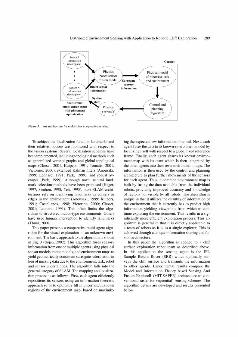
Figure 3. An architecture for multi-robot cooperative sensing.

To achieve the localization function landmarks andtheir relative motions are monitored with respect tothe vision systems. Several localization schemes havebeen implemented, including topological methods suchas generalized voronoi graphs and global topologicalmaps (Choset, 2001; Kuipers, 1991; Tomatis, 2001;Victorino, 2000), extended Kalman filters (Anousaki,1999; Leonard, 1991; Park, 1999), and robust av-erages (Park, 1999). Although novel natural land-mark selection methods have been proposed (Hager,1997; Simhon, 1998; Yeh, 1995), most SLAM archi-tectures rely on identifying landmarks as corners oredges in the environment (Anousaki, 1999; Kuipers,1991; Castellanos, 1998; Victorino, 2000; Choset,2001; Leonard, 1991). This often limits the algo-rithms to structured indoor-type environments. Othershave used human intervention to identify landmarks(Thrun, 2000).

This paper presents a cooperative multi-agent algo-rithm for the visual exploration of an unknown envi-ronment. The basic approach to the algorithm is shownin Fig. 3 (Sujan, 2002). This algorithm fuses sensoryinformation from one or multiple agents using physicalsensor models, robot models, and environment maps toyield geometrically consistent surrogate information inlieu of missing data due to the environment, task, robotand sensor uncertainties. The algorithm falls into thegeneral category of SLAM. The mapping and localiza-tion process is as follows. First, each agent efficientlyrepositions its sensors using an information theoreticapproach so as to optimally fill in uncertain/unknownregions of the environment map, based on maximiz-

ing the expected new information obtained. Next, eachagent fuses the data to its known environment model bylocalizing itself with respect to a global fixed referenceframe. Finally, each agent shares its known environ-ment map with its team which is then integrated bythe other agents into their own environment maps. Theinformation is then used by the control and planningarchitecture to plan further movements of the sensorsfor each agent. Thus, a common environment map isbuilt by fusing the data available from the individualrobots, providing improved accuracy and knowledgeof regions not visible by all robots. The algorithm isunique in that it utilizes the quantity of information ofthe environment that it currently has to predict highinformation yielding viewpoints from which to con-tinue exploring the environment. This results in a sig-nificantly more efficient exploration process. This al-gorithm is general in that it is directly applicable toa team of robots as it is to a single explorer. This isachieved through a unique information sharing and fu-sion architecture.

In this paper the algorithm is applied to a cliffsurface exploration robot team as described above.In this application the sensing agent is the JPLSample Return Rover (SRR) which optimally sur-veys the cliff surface and transmits the informationto other agents. Experimental results compare theModel and Information Theory based Sensing AndFusion ExploreR (MIT-SAFER) architecture to con-ventional raster (or sequential) sensing schemes. Thealgorithm details are developed and results presentedbelow.

290 Sujan et al.

Start

Initialize robot system(a) Initialize environment map (NULL)(b) Localize robot(c) Generate panoramic map

Select new vision system configuration for robot(a) select a test pose on plane along cliff edge(b) interpolate known data(c) evaluate probability of visibility of sub-regions(d) compute the expected new information

End criteria:Is expanse and resolution sufficient

for task requirements?

Move system into desired state(a) Execute motion command(b) Rectify true motion

N

Y

Stop

Transmit data to team(a) determine relevant data(b) compress and send

Acquire and merge new data(a) stereo map(b) uncertainty evaluation

Parameterize critical terrain features(a) determine edge as a series of pts(b) best fit points to closed polygon

Step 1

Step 2

Step 3

Step 4

Figure 4. Multi robot environment sensing and distribution flow diagram.

2. MIT-SAFER Analytical Development

In general for each sensing agent the algorithm consistsof four steps (See Fig. 4).

Step 1. System initialization: Here the environment mapis initialized, the robots are localized, and a first map isgenerated. The environment is mapped to a 2.5D eleva-tion grid, i.e., the map is a plane of grid cells where eachgrid cell value represents the average elevation of theenvironment at that cell location. This map is built ina fixed reference frame defined by a well-known land-mark measurable by all the sensing agents. All robotscontributing to or requiring use of the map are localizedwith respect to the initial map. For the cliff explorationteam, the RECON-bot contributes to and uses the en-

vironment map, while the Cliff-bot only uses the envi-ronment map. Localization may be achieved by either:

(a) Absolute localization—is achieved by mapping acommon environment landmark that is visible byall robots or

(b) Relative localization—is done by mapping fidu-cials on all robots by other robot team memberswhere one robot is selected as the origin. Relativelocalization is used in this application, with theRECON-bot localizing the Cliff-bot with respectto itself (the origin—see Fig. 5). Then, each agentinitially senses the environment.

Step2. Critical terrain feature identification: In someapplications, certain regions of the terrain may be


X

Y

Z

X

Y

(a) Orthographic view (b) Top view

Figure 5. Initial environment map coordinate frame.

critical, requiring early identification and mapping. Anexample is determining regions of safe travel for thesensing agents.

In this application, identification of the cliff edgeby the RECON-bot is critical. The edge is parameter-ized by the edge of a best-fit non-convex polygon ofthe local terrain. This permits the RECON-bot to movealong the cliff edge without falling over it. In cliff edgeparameterization, the surface currently in contact withthe RECON-bot is identified in the environment model.This surface is then approximated by a best-fit polygon.The tolerance of the fit is limited by the known roverwheel diameter, i.e., fit tolerance = wheel characteris-tic length/length per pixel. For this process the incom-plete environment model is temporarily completed bya Markovian approximation for unknown grid cells.For all unknown points a worst case initial guess isassumed. This value is the lowest elevation value cur-rently in the known model. A nearest measured neigh-bor average is performed and iterated till convergence.An example of this is shown in Fig. 6.

Using the Markovian approximation of the envi-ronment, the current rover contact surface (called theplateau) is first identified. This is achieved by setting aheight threshold bound to the environment model andprojecting the resulting data set onto the XY plane.This is followed by a region growing operation aroundthe current known rover coordinates. Next, the binaryimage is smoothed by an image closing operation (di-lation + erosion). Plateau edge pixels are easily iden-tified at this stage. However, to remove small holes inthe plateau, an edge following operation is performed.At this stage we are left with a single closed loop of

boundary pixels. Finally, this set of points is parame-terized by a closed polygon. This is initiated by fittingthe full set of boundary pixels to a straight line. For anygiven sub set of boundary pixels that is currently fit toa line, if the error bound on this fit exceeds the pre-scribed tolerance, then the pixel set is divided into two,and process is repeated. However, before error boundevaluation, line segments fit to each sub set of boundarypixels, are joined to form a closed polygon. The cliffedge parameterization algorithm is outlined in Fig. 7.

An example of the process is shown in Fig. 8 ona simulated Mars-type environment (note—simulatedenvironment is based on Viking I/II Mars lander rockdistribution statistics).

Step 3. Optimum information gathering pose selection:A rating function is used to determine the next location(position and orientation) of the sensing agent fromwhich to explore the unknown environment. The objec-tive is to acquire as much new information about the en-vironment as possible with every sensing cycle, whilemaintaining or improving the map accuracy. Hence,minimizing the exploration time. The process is con-strained by selecting goal points that are not occludedand that can be reached by a collision free feasiblepath.

The new information (NI) is equal to the expectedinformation of the unknown/partially known regionviewed from the sensor pose under consideration.In the case of the cliff surface exploration applica-tion, the sensors are CCD stereo cameras. This isbased on the known obstacles from the current en-vironment map, the field of view of the sensor and

292 Sujan et al.

Figure 6. Markovian interpolation of unknown regions.

a framework for quantifying information. Shannonshowed that the information gained by observing aspecific event among an ensemble of possible eventsmay be described by the following function (Shannon,

1948):

H (q1, q2, . . . , qn) = −n∑

k=1

qk log2 qk (1)


Start

Threshold Z data using offset from data frame to wheel frameobtain points corresponding to potential rover plateau

Select cliff edge (plateau boundary) pixels

Single closed loop of boundary pixels(a) single list of all edge points(b) nearest neighbor pick within prescribed distance limit

Stop

Best polygon fit (1/3)(a) select whole edge point set(b) line best fit

Obtain main rover plateau(a) obtain rover current location (Xr, Yr)(b) region growing applied about (Xr, Yr)

Close main plateau(a) binary dilate(b) binary erode

Is fit tolerance at each edge

adequate?

Return best fit polygon

Best polygon fit (3/3)(a) binary divide point set with poor tolerance(b) line best fit for both sub point sets(c) sort line segs. based on associated edge point set(d) connect line segs. end points

Best polygon fit (2/3)(a) RMS evaluate each line segment

Figure 7. Cliff edge parameterization algorithm flow diagram.

where qk represents the probability of occurrence forthe kth event. This definition of information may alsobe interpreted as the minimum number of states (bits)needed to fully describe a piece of data. Shannon’semphasis was in describing the information content

of 1-D signals. In 2-D the gray level histogram ofan ergodic image can be used to define a probabilitydistribution:

qi = fi/N for i = 1 . . . Ngray (2)

294 Sujan et al.

where fi is the number of pixels in the image with graylevel i , N is the total number of pixels in the image,and Ngray is the number of possible gray levels. Withthis definition, the information of an image for whichall the qi are the same—corresponding to a uniform

Figure 8. Example of cliff edge parameterization.(Continued on next page.)

gray level distribution or maximum contrast—is a max-imum. The less uniform the histogram, the lower theinformation.

It has been shown that it is possible to extend thisidea of information to a 3-D signal (Sujan, 2002). In this


Figure 8. (Continued).

paper this idea is extended to a 2.5D signal—environment elevation map. The new information con-tent for a given sesnor (camera) view pose is given by:

H(camx,y,z,θp,θy

) =∑

i

nmaxgrid − ni

grid

nmaxgrid

{(Pi

V

2log2

PiV

2

)

+(

1 − PiV

2log2

(1 − Pi

V

2

))}(3)

where H is summed over all grid cells, i , visible fromcamera pose camx,y,z,θp,θy ; ni

gridis the number of envi-ronment points measured and mapped to cell i ; nmax

grid isthe maximum allowable mappings to cell i ; and Pi

V isthe probability of visibility of cell i from the cameratest pose.

A single range observation of a point (x) is modeledas a 3-D Gaussian probability distribution centered atx , based on two important observations. First, the useof the mean and covariance of a probability distributionfunction is a reasonable form to model sensor data andis a second order linear approximation (Smith, 1986).This linear approximation corresponds to the use of aGaussian (having all higher moments of zero). Second,from the central limit theorem, the sum of a number ofindependent variables has a Gaussian distribution re-gardless of their individual distributions. The standard

deviations along the three axes of the distribution cor-respond to estimates of the uncertainty in the range ob-servation along these axes. These standard deviationsare a function of intrinsic sensor parameters (such ascamera lens shape accuracy) as well as extrinsic sensorparameters (such as the distance to the observed pointor feature). For most range sensing systems, this modelcan be approximated as (Sujan, 2002):

σx,y,z = f (extrinsic parameters, intrinsic parameters)

≈ S · Tx,y,z · Ln (4)

where S is an intrinsic parameter uncertainty constant,Tx,y,z is an extrinsic parameter uncertainty constant, Lis the distance to the feature/environment point, and nis a constant (typically 2).

PiV is evaluated by computing the likelihood of oc-

clusion of a ray rayx,y,z using the elevation, Obx,y,z ,and the associated uncertainty, σx,y,z , at all cells lyingalong this ray path shot through each position in theenvironment grid to the camera center. From Fig. 9, ifgrid cell i falls within the camera field of view, thenits average elevation, Ptx,y,z (obtained either as an av-erage of all measured points mapped to cell i , or asthe Markovian approximation of its neighborhood ifno points have currently been mapped to cell i) traces

296 Sujan et al.

Figure 9. Ray tracing to determine probability of visibility of a grid cell from a given camera configuration.

a ray to the camera center, Camx,y,z. PiV is given by:

PiV =

∏�x

{sgn(rayz − Obz)

·∫ (rayz−Obz)

0

1

σz

√2π

exp

(− z2

2σz

)dz + 0.5

}(5)

This definition for NI has an intuitively correct form.Regions with higher visibility and associated higherlevel of unknowns yield a higher expected NI value.Higher occlusions or better known regions result inlower expected NI values.

During the mapping process some regions that areexpected to be visible may not be, because of sensorcharacteristics (e.g., lack of stereo correspondence dueto poor textures or lighting conditions), and inaccu-racies in the data model (e.g., expected neighboringcell elevations and uncertainties—occlusions). How-ever, after repeated unsuccessful measurements of cellsexpected to be visible, it becomes more likely that sen-sor characteristics are the limitation. This is representedas a data quality function that reduces as the numberof unsuccessful measurements of the visible cell in-creases. The probability of visibility of the cell i , Pi

V ,

is pre-multiplied by a “interest function,” I.F., for thecell i given at the kth unsuccessful measurement by:

I.F.0i = 1(6)

I.F.ki = 1

eβ PiV

· I.F.k−1i

where β is a scaling constant determined empirically—larger values result in faster decrease of I.F. Note thatcells with low Pi

V resulting in an unsuccessful measure-ment are not as severly penalized as cells with high Pi

V .Hence, occluded regions do not translate to low dataquality regions. This permits future “interest” in suchregions that may be explored later.

Data fusion: A final step in environment map buildingis to fuse the newly acquired data by each agent withthe environment model currently available to that agent.Each agent only fuses its own newly acquired data tothe environment map stored in its memory. Thus asthe environment map develops on an individual agentlevel, it needs to be shared and integrated among theteam to keep each agent updated. Optimal map sharingprotocols for multi agent systems is currently work inprogress, i.e., decentralized protocols instructing theteam members when and how to share their individual


g01

Target frameCamera base

frame x

y

z

xy

z

rk(u,v,f)

(u,v)f

Spatial point

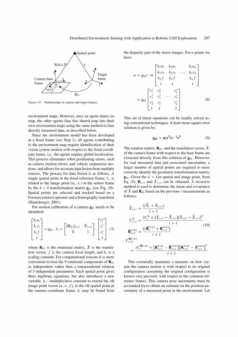
Figure 10. Relationship of camera and target frames.

environment maps. However, once an agent shares itsmap, the other agents fuse this shared map into theirown environment maps using the same method to fusedirectly measured data, as described below.

Since the environment model has been developedin a fixed frame (see Step 1), all agents contributingto the environment map require identification of theirvision system motion with respect to the fixed coordi-nate frame, i.e., the agents require global localization.This process eliminates robot positioning errors, suchas camera motion errors, and vehicle suspension mo-tions, and allows for accurate data fusion from multiplesources. The process for data fusion is as follows. Asingle spatial point in the fixed reference frame, ri , isrelated to the image point (ui , vi ) in the sensor frameby the 4 × 4 transformation matrix g01 (see Fig. 10).Spatial points are selected and tracked based on aForstner interest operator and a homography transform(Huntsberger, 2001).

For motion calibration of a camera g01 needs to beidentified:

ki ui

kivi

ki f

1

= g01 · ri =

[[R01]3×3 X3×1

0 1

]·

r xi

r yi

r zi

1

(7)

where R01 is the rotational matrix, X is the transla-tion vector, f is the camera focal length, and ki is ascaling constant. For computational reasons it is moreconvenient to treat the 9 rotational components of R01

as independent, rather than a transcendental relationof 3 independent parameters. Each spatial point givesthree algebraic equations, but also introduces a newvariable, ki —multiplicative constant to extend the i thimage point vector (u, v, f )i to the i th spatial point inthe camera coordinate frame. ki may be found from

the disparity pair of the stereo images. For n points wehave:

u = g01r ⇒

k1u1 k2u2 knun

k1v1 k2v2 · · · knvn

k1 f k2 f kn f

1 1 1

= g01

r x1 r x

2 r xn

r y1 r y

2 · · · r yn

r z1 r z

2 r zn

1 1 1

(8)

This set of linear equations can be readily solved us-ing conventional techniques. A least mean square errorsolution is given by:

g01 = u(rTr)−1rT (9)

The rotation matrix, R01, and the translation vector, X ,of the camera frame with respect to the base frame areextracted directly from this solution of g01. However,for real measured data and associated uncertainty, alarger number of spatial points are required to morecorrectly identify the geometric transformation matrix,g01. Given the (i + 1)st spatial and image point, fromEq. (9), Ri+1 and X i+1 can be obtained. A recursivemethod is used to determine the mean and covarianceof X and R01 based on the previous i measurements asfollows:

ˆXi+1 = (i ˆXi + Xi+1)

i + 1

C Xi+1 = iC X

i + [Xi+1 − ˆXi+1][Xi+1 − ˆXi+1]T

i + 1 (10)

R(l,m)i+1 =

(iR(l,m)

i + R(l,m)i+1

)i + 1

CR(l,m)i+1

= iCR(l,m)i + [

R(l,m)i+1 − R(l,m)

i+1

][R(l,m)

i+1 − R(l,m)i+1

]T

i + 1

This essentially maintains a measure on how cer-tain the camera motion is with respect to its originalconfiguration (assuming the original configuration isknown very precisely with respect to the common ref-erence frame). This camera pose uncertainty must beaccounted for to obtain an estimate on the position un-certainty of a measured point in the environment. Let

298 Sujan et al.

the measurement z be related to the state vector (ac-tual point position) x by a non-linear function, h(x).The measurement vector is corrupted by a sensor noisevector v of known covariance matrix, R.

z = h(x) + v (11)

Assume that the measurement of the state vector x isdone multiple times. In terms of the current measure-ment, a Jacobian matrix of the measurement relation-ship evaluated at the current state estimate is definedas:

Hk = ∂h(x)

∂ x

∣∣∣∣x=xk

(12)

The state (or positition) may then be estimated as fol-lows:

Kk = Pk H Tk

[Hk Pk H T

k + Rk]−1

ˆxk+1 = ˆxk + Kk[zk − h(xk)] (13)

Pk+1 = [1 − Kk Hk]Pk

This estimate is known as the Extended Kalman Filter(Gelb, 1974). Using this updated value for both themeasured point x and the absolute uncertainty P , themeasured point may then be merged with the currentenvrionment model.

Provided two observations are drawn from a normaldistribution, the observations can be merged into an im-proved estimate by multiplying the distributions. Sincethe result of multiplying two Gaussian distributions isanother Gaussian distribution, the operation is symmet-ric, associative, and can be used to combine any numberof distributions in any order. The canonical form of theGaussian distribution in n dimensions depends on thestandard distributions, σx,y,z , a covariance matrix (C)and the mean (x) (Stroupe, 2000; Smith, 1986):

p(x ′ | y)

= 1

(2π )n/2√|C |exp

(−1

2(y − x ′)T C−1(y − x ′)

)

where

C =

σ 2x ρxyσxyσxy ρzxσzxσzx

ρxyσxyσxy σ 2y ρyzσyzσyz

ρzxσzxσzx ρyzσyzσyz σ 2z

(14)

where the exponent is called the Mahalanobis distance.For un-correlated measured data ρ = 0. The formu-lation in Eq. (14) is in the spatial coordinate frame.However, all measurements are made in the camera (orsensor) coordinate frame. This problem is addressedthrough a transformation of parameters from the obser-vation frame to the spatial reference frame as follows:

Ctransformed = R(−θ )T · C · R(−θ ) (15)

where R( θ ) the rotation matrix between the two coor-dinate frames. The angle of the resulting principal axiscan be obtained from the merged covariance matrix:

Cmerged = C1(I − C1(C1 + C2)−1) (16)

where Ci is the covariance matrix associated with thei th measurement. Additionally, a translation operationis applied to the result from Eq. (14), to bring the resultinto the spatial reference frame. To contribute to theprobabilistic occupancy environment model, all mea-sured points corresponding to obstacles are merged.That is, all measured points falling in a particular gridcell, contribute to the error analysis associated with thatvoxel.

Note that adding noisy measurements leads to a nois-ier result. For example, the camera pose uncertaintyincreases as the number of camera steps increase. Withevery new step, the current uncertainty is merged withthe previous uncertainty to get an absolute uncertaintyin camera pose. However, by merging (multiplying) re-dundant measurements (filtering) leads to a less noisierresult (e.g., the environment point measurements).

In addition to maximizing information acquisition,it is also desirable to minimize travel distance andmaintain/improve the map accuracy, while being con-strained to move along feasible paths. A Euclidean met-ric in configuration space, with individual weights αi

on each degree of freedom of the camera pose c, is usedto define the distance moved by the camera:

d =(

n∑i=1

αi (ci − c′i )

2

)1/2

(17)

where c and c′ are vectors of the new and current cameraposes respectively. Here αi is set to unity. In generalthis parameter reflects the ease/difficulty in moving thevision system in the respective axis. Map accuracy isbased on the accuracy of localization of each sensingagent. This may be obtained by adding the localization


error of the agent along the path to the target. Pathscontaining more promising fiducials for localizationresult in higher utility in determining both the goallocation and the path to the goal. The new information,the travel distance and the net improvement of mapaccuracy is combined into a single utility function thatmay be optimized to select the next view pose.

Step 4. Map distribution: As each agent maps andfuses an environment section to the environment map,it needs to distribute this updated map among the otheragents. This is required so that each agent may opti-mally plan its next move and add information to themap. Once completed, the environment map needs tobe distributed to the team. For example, to explore thecliff, after the RECON-bot has developed the geomet-rical cliff surface map, it needs to transfer this to theCliff-bot for task execution (e.g., science instrumentplacement) (Huntsberger, 2001; Huntsberger, 2003).

Due to communication bandwidth limitationsof NASA/JPL present and near-term rovers, anappropriate data transfer algorithm needs to bedeveloped. For example, during the 1997 MarsSojourner mission, both the lander and rover car-ried 9600 baud radio modems, with an effectivedata rate of 2400 bps (http://mars.jpl.nasa.gov/MPF/rover/faqs sojourner.html). For the 2003 MarsExploration Rover (MER) mission the datatransfer rates of MER-to-Earth is expected tovary from 3 Kbps to 12 Kbps and MER-to-orbiter is expected to stay constant at 128 Kbps(http://mars.jpl.nasa.gov/mer/mission/comm data.html<x-html>). These communication limitations maybe further exacerbated with multiple cooperatingagents. Thus successful communication requires thereduction of the data set into relevant data, i.e., onlycommunicate data that is necessary for task execution.

The data reduction algorithm used here breaks downthe environment map into a quadtree of interest regions.This is achieved by first reducing the entire elevationmap with adaptive decimation. This removes highly in-significant objects, such as small pebbles. The resultingdata set is divided into four quadrants. The informationcontent of each quadrant is evaluated using Eqs. (1)and (2). This information content reflects the amountof variation in the terrain quadrant (where higher infor-mation content signifies higher variation in the terrain).Quadrants with high information content are further di-vided into sub-quadrants and the evaluation process iscontinued. Once it is determined that a quadrant does

Start

Data convolved with low pass filter(remove high frequency noise)

Quadtree decomposition of compressed data set(quad divided iif information content of any subquad

> information content of current quad)

Base transmission data (BTD) set formed(a) coordinates of quadtree nodes(b) value of quadtree node = avg(quad value)

Stop

Transmit data to Cliffbot(a) wireless handshaking(b) bit-sum checking

Conventional compression of BTD using lossless compression algorithm

Data reduced using adaptive decimation(removes objects insignificant to rover wheel base clearnace)

Lossless data compression(using predictive compression algorithm)

Figure 11. Inter-robot communication flow diagram.

not require further subdivision, an average elevationvalue of the particular quadrant is used for transmis-sion (rather than the elevation of all grid cells withinthat quadrant). This cutoff threshold of information isbased on a critical robot physical parameter (e.g., thewheel diameter). This results in a significantly reduceddata set known as the quadtree of interest regions. Con-ventional lossless compression schemes may then beapplied to the reduced data set to further reduce thenumber of transmission bits. The flow diagram of thisprocess is given in Fig. 11.

3. Experimental Results

The basic MIT-SAFER algorithm was applied to the co-operative exploration of cliff surfaces by a team of fourrobots. The JPL Sample Return Rover (SRR) served

300 Sujan et al.

Figure 12. Experimental laboratory setup.

as the RECONbot for this application. The SRR is afour-wheeled mobile robot with independently steeredwheels and independently controlled shoulder joints.It carries a stereo pair of cameras mounted on a threeDOF articulated manipulator. The SRR is equippedwith a 266 MHz PC-104 computer platform, operat-ing with VX-Works. Five mapping techniques, includ-ing the one developed above, were implemented. Thesewere: These include:

Method 1. Raster scanning without yaw.Method 2. Raster scanning with yaw.Method 3. Information based environment mapping

with cliff edge assumed to be a straight line segment.Method 4. Information based environment mapping

with cliff edge approximated as a non-convex poly-gon.

Method 5. Information based environment mappingwith interest function and cliff edge approximatedas a non-convex polygon.

The first two methods reflect commonly used envi-ronment mapping schemes (Asada, 1990; Burschka,1997; Castellanos, 1998; Choset, 2001; Kuipers, 1991;Rekleitis, 2000; Victorino, 2000). The latter three re-flect with increased complexity the algorithm devel-oped here.

The experimental setup for the first study in the Plan-etary Robotics Lab (PRL) at JPL is shown in Fig. 12.A recessed sandpit containing several rock piles ismapped. The edge of the sandpit, a vertical drop, acts asthe cliff edge. This limits the motion of the RECON-botto lie in the flat plane behind the cliff edge (see Fig. 12).Figure 13 shows the number of environment grid cellsexplored as a function of the number of stereo imag-ing steps. From this experimental study, the improvedefficiency of the method presented in this paper overconventional raster scanning methods can be seen, withan order of magnitude more points being mapped byMethod 5 over those returned from Method 1 for thesame number of stereo imaging steps. A significant im-provement in efficiency can be seen while progressingfrom Method 3 to Method 5. In Method 4, by param-eterizing the cliff edge, the rover is able to follow theedge more aggressively, thus covering a larger varietyof view points.

Figure 14 shows a top view of the environment pointsmapped using Methods 3 and 5. It is seen that Method 5takes approximately half the number of steps to map aqualitatively similar region. Further, it is observed thatthe left region of the sandpit in Fig. 12 yields poor data(due to lack of stereo correspondence). Since this re-gion is expected have high information content (due tolack of occlusions), the algorithm in Method 3 tendsto converge to view points looking in that direction.


Figure 13. Amount of environment explored.

Figure 14. Top view of mapped points.

302 Sujan et al.

0 2 4 6 8 10 12 14 16 18 200

500

1000

1500

2000

2500

3000

3500

Number of Stereo Imaging Steps

Nu

mb

er o

f M

app

ed G

rid

Cel

ls

Maximum Information

Expected number of new mapped cellsObtained number of new mapped cells

0 2 4 6 8 10 12 14 16 18 200

500

1000

1500

2000

2500

3000

Number of stereo imaging steps

Nu

mb

er o

f m

app

ed g

rid

cel

ls

Maximum Information + Cliff Edge Parameterization + Interest Function

Expected number of new mapped cellsObtained number of new mapped cells

(a) Method 3 (b) Method 5

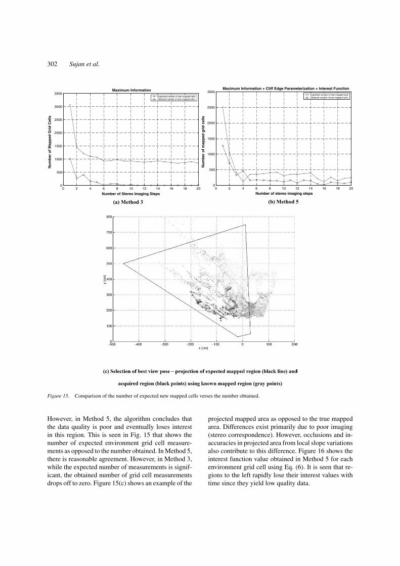
Figure 15. Comparison of the number of expected new mapped cells verses the number obtained.

However, in Method 5, the algorithm concludes thatthe data quality is poor and eventually loses interestin this region. This is seen in Fig. 15 that shows thenumber of expected environment grid cell measure-ments as opposed to the number obtained. In Method 5,there is reasonable agreement. However, in Method 3,while the expected number of measurements is signif-icant, the obtained number of grid cell measurementsdrops off to zero. Figure 15(c) shows an example of the

projected mapped area as opposed to the true mappedarea. Differences exist primarily due to poor imaging(stereo correspondence). However, occlusions and in-accuracies in projected area from local slope variationsalso contribute to this difference. Figure 16 shows theinterest function value obtained in Method 5 for eachenvironment grid cell using Eq. (6). It is seen that re-gions to the left rapidly lose their interest values withtime since they yield low quality data.


Figure 16. Interest function value after 10 steps using Method 5.

Figure 17. Experimental field system setup.

Field tests were conducted near the Tujunga Damin Tujunga, CA on a natural cliff face with a verticalslope of ∼75◦. This setup seen in Fig. 17. This is thephysical realization of the conceptual description pro-vided in Section 1 of a team of four cooperating robotsexploring a cliff surface. Due to time constraints, ex-

perimental tests could only be run for Method 3 usingthe maximum information content and Method 5 usingthe maximum information content with interest func-tion. The results of the study for 10 imaging steps areshown in Fig. 18. Figure 19 shows part of the cliff sur-face and its corresponding map. Of particular interest

304 Sujan et al.

Figure 18. Amount of environment explored.

Figure 19. Tujunga dam cliff site.

is the rock jumble to the Cliffbot, which may chooseto avoid it during traversal.

Figure 20 compares the number of expected environ-ment grid cell measurements and the number obtainedfor the two methods. Method 5 shows reasonable agree-ment, while Method 3 results in a large discrepancy.Once again, differences exist primarily due to poorimaging (stereo correspondence). However, occlusions

and inaccuracies in projected area from local slope vari-ations also contribute to this difference. Finally, Fig. 21shows the interest function value obtained in Method 5for each environment grid cell using Eq. (6).

These results demonstrate the effectiveness of themulti-agent environment mapping architecture devel-oped in this paper. To demonstrate the effectiveness ofthe map reduction and distribution algorithm for robots


1 2 3 4 5 6 7 8 9 100

500

1000

1500

2000

2500

3000

3500

4000

4500

5000


Num

ber

of m

appe

d gr

id c

ells

Expected number of new grid cellsObtained number of new grid cells

1 2 3 4 5 6 7 8 9 100

500

1000

1500

2000

2500

3000

3500

4000

4500

5000


Num

ber

of m

appe

d gr

id c

ells

Expected number of new grid cellsObtained number of new grid cells

(a) Method 3 (b) Method 5

Figure 20. Comparison of the number of expected new mapped cells verses the number obtained.

Figure 21. Interest function value after 10 steps using Method 5.

in real Mars field environments, 32 different elevationmaps of fixed dimensions, based on the statistics ofViking I/II Mars lander data were tested. The data ofeach elevation map was reduced with respect to a robotwith varying wheel diameter. To compare the data re-duction, a terrain variation parameter, dH, is definedas the terrain elevation variation normalized by therobot wheel diameter. Thus, it is expected that robotswith smaller wheel diameters (higher dH) require agreater amount of terrain detail for navigation, thanthose with larger wheel diameters for the same terrainmap. Figure 22 confirms this expectation. It shows the

data reduction factor as a function of dH using the algo-rithm described above (without conventional losslesscompression added at the end). The variation at eachdata point represents the variation in data reduction ex-pected for a given elevation map.

An example of this data reduction process is shown inFigs. 23–26. It compares the grayscale elevation mapbefore and after the data reduction process—lighterregions indicate higher elevations. Figure 23 shows acontour map of the simulated environment. Figure 24shows the quad-tree decomposition of the environment.Note that higher divisions of regions indicate more

306 Sujan et al.

0 5 10 15 20 25 30 350

5

10

15

20

25

30

Terrain dh (units = rover clearance height)

Ave

rage

dat

a re

duct

ion

ratio

Figure 22. Elevation map data reduction for transmission as a function of terrain elevation range.

Figure 23. Simulated world contour map—gray color code indicates darker regions to be of lower elevation.


Figure 24. Quadtree decomposition of elevation map.

Figure 25. Quadtree decomposition overlaid on original elevation map.

308 Sujan et al.

Figure 26. The original (left) and the process/transmitted (right) environment elevation maps.

complex terrain and consequently higher relevant in-formation content. Figure 25 shows the contour mapoverlaid on the original grayscale elevation map. Fi-nally, Fig. 26 compares the elevation map before andafter the data reduction process.

For this example, a data reduction factor of ap-proximately 10 was achieved with a dH = 8. Al-though visually the left and right images of Fig. 26may appear the same, closer inspection reveals re-gions in the transmitted image (such as the bottomright corner) to contain very little information con-tent. This indicates that the region in the original ele-vation contained insignificant terrain variation with re-spect to the particular wheel diameter. However, otherregions such as the boulders, indicated in the origi-nal elevation map, that are critical with respect to thewheel diameter, are faithfully transmitted. It is seenthat using this method, significant data reduction can beachieved while maintaining the overall map structure.Although, this is applied to a 2.5D environment eleva-tion map here, the algorithm is directly applicable to3D maps.

4. Conclusions

This paper has presented a cooperative multi-agent dis-tributed sensing architecture. This algorithm efficientlyrepositions the systems’ sensors using an informationtheoretic approach and fuses sensory information fromthe agents using physical models to yield a geomet-rically consistent environment map. This map is then

distributed using an information based relevant data re-duction scheme for communication. The architectureis proposed for a team of robots cooperatively inter-acting to explore a cliff face. Experimental results us-ing the JPL Sample Return Rover (SRR) have beenpresented. This single rover acts as a surveyor, opti-mally generating a map of the cliff face. The method isshown to significantly improve the environment map-ping efficiency. The algorithm shows additional map-ping efficiency improvement when an interest functionis included. This function measures the data quality inthe environment. Future work includes implementationand testing of the inter-robot communication algorithmon the experimental platform.

Acknowledgments

The authors would like to acknowledge the support ofthe Jet Propulsion Laboratory, NASA under contractnumber 1216342.

References

Anousaki, G.C. and Kyriakopoulos, K.J. 1999. Simultaneous lo-calization and map building for mobile robot navigation. IEEERobotics & Automation Magazine, 6(3):42–53.

Asada, M. 1990. Map building for a mobile robot from sensorydata. IEEE Transactions on Systems, Man, and Cybernetics,37(6).

Baumgartner, E.T., Schenker, P.S., Leger, C., and Huntsberger, T.L.1998. Sensor-fused navigation and manipulation from a plane-tary rover. In Proceedings of SPIE Symposium on Sensor Fusion


and Decentralized Control in Robotic Systems, Boston, MA,vol. 3523.

Burschka, D., Eberst, C., and Robl, C. 1997. Vision based modelgeneration for indoor environments. In Proceedings of the 1997IEEE International Conference on Robotics and Automation,Albuquerque, New Mexico, vol. 3, pp. 1940–1945.

Castellanos, J.A., Martinez, J.M., Neira, J., and Tardos, J.D. 1998.Simultaneous map building and localization for mobile robots:A multisensor fusion approach. In Proceedings of 1998 IEEEInternational Conference on Robotics and Automation, Leuven,Belgium, vol. 2, pp. 1244–1249.

Choset, H. and Nagatani, K. 2001. Topological simultaneous local-ization and mapping (SLAM): Toward exact localization withoutexplicit localization. IEEE Transactions on Robotics and Automa-tion, 17(2):125–137.

Gelb, A. 1974. Applied Optimal Estimation. MIT Press: Cambridge,Massachusetts, U.S.A.

Hager, G.D., Kriegman, D., Teh, E., and Rasmussen, C. 1997. Image-based prediction of landmark features for mobile robot navigation.In Proceedings of the 1997 IEEE International Conference onRobotics and Automation, Albuquerque, New Mexico, vol. 2, pp.1040–1046.

Huntsberger, T.L., Rodriguez, G., and Schenker, P.S. 2000. Robotics:Challenges for robotic and human Mars exploration. In Proceed-ings of ROBOTICS2000, Albuquerque, New Mexico, pp. 299–305.

Huntsberger, T.L., Pirjanian, P., and Schenker, P.S. 2001. Roboticoutposts as precursors to a manned Mars habitat. In Proceedings ofthe 2001 Space Technology and Applications International Forum(STAIF-2001), Albuquerque, New Mexico, pp. 46–51.

Huntsberger, T.L., Sujan, V.A., Dubowsky, S., and Schenker, P.S.2003. Integrated system for sensing and traverse of cliff faces. InProceedings of Aerosense’03: Unmanned Ground Vehicle Tech-nology V. SPIE, Orlando, Florida, vol. 5083.

Kruse, E., Gutsche, R., and Wahl, F.M. 1996. Efficient, iterative, sen-sor based 3-D map building using rating functions in configurationspace. In Proceedings of the 1996 IEEE International Conferenceon Robotics and Automation, Minneapolis, Minnesota, vol. 2, pp.1067–1072.

Kuipers, B. and Byun, Y. 1991. A robot exploration and mappingstrategy based on semantic hierarchy of spatial representations.Journal of Robotics and Autonomous Systems, 8:47–63.

Leonard, J.J. and Durrant-Whyte, H.F. 1991. Simultaneous mapbuilding and localization for an autonomous mobile robot. In IEEE1991 International Workshop on Intelligent Robots and Systems,Osaka, Japan, vol. 3, pp. 1442–1447.

Lumelsky, V., Mukhopadhyay, S., and Sun, K. 1989. Sensor-basedterrain acquisition: The “sightseer” strategy. In Proceedings of the28th Conference on Decision and Control, Tampa, Florida, vol. 2,pp. 1157–1161.

Osborn, J.F., Whittaker, W.L., and Coppersmith, S. 1987. Prospectsfor robotics in hazardous waste management. In Proceedings of theSecond International Conference on New Frontiers for HazardousWaste Management, Pittsburgh, Pennsylvania.

Park J., Jiang, B., and Neumann, U. 1999. Vision-based pose com-putation: Robust and accurate augmented reality tracking. In Pro-ceedings of the 2nd IEEE/ACM International Workshop on Aug-mented Reality, San Francisco, California, pp. 3–12.

Pirjanian, P., Huntsberger, T.L., and Schenker, P.S. 2001. Develop-ment of CAMPOUT and its further applications to planetary rover

operations: A multirobot control architecture. In Proceedings ofSPIE Sensor Fusion and Decentralized Control in Robotic SystemsIV, Newton, Massachusetts, vol. 4571, pp. 108–119.

Rekleitis, I., Dudek, G., and Milios, E. 2000. Multi-robot collabora-tion for robust exploration. In Proceedings of the 2000 IEEE Inter-national Conference on Robotics and Automation, San Francisco,California, vol. 4, pp. 3164–3169.

Schenker, P.S., Baumgartner, E.T., Lindemann, R.A., Aghazarian, H.,Ganino, A.J., Hickey, G.S., Zhu, D.Q., Matthies, L.H., Hoffman,B.H., and Huntsberger, T.L. 1998. New planetary rovers for long-range Mars science and sample return. In Proceedings of SPIESymposium on Intelligent Robots and Computer Vision XVII: Al-gorithms, Techniques, and Active Vision, Boston, Massachusetts,vol. 3522.

Schenker, P.S., Pirjanian, P., Huntsberger, T.L., Trebi-Ollennu, A.,Aghazarian, H., Leger, C. JPL, Dubowsky, S. MIT, McKee,G.T., University of Reading (UK). 2001. Robotic intelligence forspace: Planetary surface exploration, task-driven robotic adapta-tion, and multirobot cooperation. In Proceedings of SPIE Sym-posium on Intelligent Robots and Computer Vision XX: Algo-rithms, Techniques, and Active Vision, Newton, Massachusetts,vol. 4572.

Shaffer, G. and Stentz, A. 1992. A robotic system for undergroundcoal mining. In Proceedings of 1992 IEEE International Con-ference on Robotics and Automation, Nice, France, vol. 1, pp.633–638.

Shannon, C.E. 1948. A mathematical theory of communication. TheBell System Technical Journal, 27:379–423.

Simhon, S. and Dudek, G. 1998. Selecting targets for local referenceframes. In Proceedings of the 1998 IEEE International Conferenceon Robotics and Automation, Leuven, Belgium, vol. 4, pp. 2840–2845.

Smith, R.C. and Cheeseman, P. 1986. On the representation andestimation of spatial uncertainty. International Journal of RoboticsResearch, 5(4):56–68.

Stroupe, A.W., Martin, M., and Balch, T. 2000. Merging gaussiandistributions for object localization in multi-robot systems. In Pro-ceedings of the Seventh International Symposium on ExperimentalRobotics, ISER ‘00, Hawaii.

Sujan, V.A. and Dubowsky, S. 2002. Visually built task models forrobot teams in unstructured environments. In Proceedings of the2002 IEEE International Conference on Robotics and Automation,Washington, DC, vol. 2, pp. 1782–1787.

Thrun, S., Burgard, W., and Fox, D. 2000. A real-time algorithmfor mobile robot mapping with applications to multi-robot and 3Dmapping. In Proceedings of the 2000 IEEE International Con-ference on Robotics and Automation, San Francisco, California,vol. 1, pp. 321–328.

Tomatis, N., Nourbakhsh, I., and Siegwar, R. 2001. Simultaneouslocalization and map building: A global topological model withlocal metric maps. In Proceedings of IEEE/RSJ International Con-ference on Intelligent Robots and Systems, Maui, Hawaii, vol. 1,pp. 421–426.

Trebi-Ollennu, A., Das, H., Aghazarian, H., Ganino, A., Pirjanian, P.,Huntsberger, T., and Schenker, P. 2002. Mars rover pair coopera-tively transporting a long payload. In Proceedings of 2002 IEEE In-ternational Conference on Robotics and Automation, Washington,DC, vol. 4, pp. 3136–3141.

Victorino, A.C., Rives, P., and Borrelly, J.-J. 2000. Localization andmap building using a sensor-based control strategy. In Proceedings

310 Sujan et al.

of 2000 IEEE/RSJ International Conference on Intelligent Robotsand Systems, Takamatsu, Japan, vol. 2, pp. 937–942.

Yamauchi, B., Schultz, A., and Adams, W. 1998. Mobile robot ex-ploration and map-building with continuous localization. In Pro-ceedings of 1998 IEEE International Conference on Robotics andAutomation, Leuven, Belgium, vol. 4, pp. 3715–3720.

Yeh, E. and Kriegman, D.J. 1995. Toward selecting and recognizingnatural landmarks. In Proceedings of the 1995 IEEE/RSJ Interna-tional Conference on Intelligent Robots and Systems, Pittsburgh,Pennsylvania, vol. 1, pp. 47–53.

Vivek Sujan received his B.S. in Physics and Mathematics summacum laude from the Ohio Wesleyan University in 1996, his B.S. inMechanical Engineering, with honors from the California Instituteof Technology, 1996, and his M.S. and Ph.D. in Mechanical En-gineering from the Massachusetts Institute of Technology in 1998and 2002 respectively. He is currently a Post-Doctoral Associate inMechanical Engineering at M.I.T. Research interests include the de-sign, dynamics and control of electromechanical systems; mobilerobots and manipulator systems; optical systems and sensor fusionfor robot control; image analysis and processing. He has been electedto Sigma Xi (Research Honorary Society), Tau Beta Pi (Engineer-ing Honorary Society), Phi Beta Kappa (Senior Honorary Society),Sigma Pi Sigma (Physics Honorary Society), Pi Mu Epsilon (MathHonorary Society).

Steven Dubowsky received his Bachelor’s degree from RensselaerPolytechnic Institute of Troy, New York in 1963, and his M.S. andSc.D. degrees from Columbia University in 1964 and 1971. He iscurrently a Professor of Mechanical Engineering at M.I.T. He hasbeen a Professor of Engineering and Applied Science at the Uni-versity of California, Los Angeles, a Visiting Professor at Cam-bridge University, Cambridge, England, and Visiting Professor atthe California Institute of Technology. During the period from 1963to 1971, he was employed by the Perkin-Elmer Corporation, theGeneral Dynamics Corporation, and the American Electric PowerService Corporation. Dr. Dubowsky’s research has included the de-

velopment of modeling techniques for manipulator flexibility andthe development of optimal and self-learning adaptive control pro-cedures for rigid and flexible robotic manipulators. He has authoredor co-authored nearly 200 papers in the area of the dynamics, controland design of high performance mechanical and electromechanicalsystems. Professor Dubowsky is a registered Professional Engineerin the State of California and has served as an advisor to the NationalScience Foundation, the National Academy of Science/Engineering,the Department of Energy, and the US Army. He has been elected afellow of the ASME and IEEE and is a member of Sigma Xi, andTau Beta Pi.

Terry Huntsberger is a Senior Member of the Technical Staff inthe Mechanical and Robotics Technologies Group at NASA’s JetPropulsion Laboratory in Pasadena, CA, where he is the Managerfor numerous tasks in the areas of multi-robot control systems, roversystems for access to high risk terrain, and long range traverse al-gorithms for rovers. He is a member of the planning teams forthe Mars Science Laboratory (MSL) mission planned for launch in2009. He is an Adjunct Professor and former Director of the Intel-ligent Systems Laboratory in the Department of Computer Scienceat the University of South Carolina. His research interests includebehavior-based control, computer vision, neural networks, wavelets,and bio-logically inspired system design. Dr. Huntsberger has pub-lished over 100 technical articles in these and associated areas. Hereceived his PhD in Physics in 1978 from the University of South Car-olina. He is a member of SPIE, ACM, IEEE Computer Society, andINNS.

Hrand Aghazarian is a Senior Member of the Engineering Staff inthe Mechanical sand Robotics Technologies Group at the Jet Propul-sion Laboratory in Pasadena, CA. He has extensive work experiencein the design and development of real-time embedded software fora variety of avionics systems. Currently he is involved in provid-ing software solutions in the area of software architecture, low-leveldrivers, motor control, user interfaces for commanding planetary


rovers, and navigation algorithm for SRR and FIDO rovers. His re-search interests are Rover Navigation/Control and Real-Time Em-bedded software Design and Development. He received a dual B.S.degree in Applied Math and Computer Science and a M.S. degree inComputer Science from California State University in Northridge.He is a member of ACM and INNS.

Yang Cheng is a senior research staff member in the Machine Vi-sion Group of the Jet Propulsion Laboratory. He earned his Ph.D. inremote sensing from the Geography Department of the University ofSouth Carolina and was then a staff member at Oak Ridge NationalLaboratory. Since coming to JPL in 1999, he has worked on severalspace robotic research projects, including Landmark-Based SmallBody Navigation System, the Vision and Navigation Subsystem forthe FIDO rover, and Passive Imaging-Based Spacecraft Safe Land-ing. Yang’s research interests include robotic navigational autonomy,computer vision, remote sensing, cartography, map projection, geo-graphic information systems, parallel computing, etc.

Paul S. Schenker is Manager, Mobility Systems Concept Develop-ment Section, Jet Propulsion Laboratory (JPL), California Instituteof Technology, Pasadena, and as such, responsible for JPL R&D inplanetary mobility and robotics. His published research includes top-ics in robotic perception, robot control architectures, telerobotics andteleoperation, multi-sensor fusion, and most recently, multi-robot co-operation. He has led the development of robotic systems that includethe Field Integrated Design & Operations Rover (FIDO), Plan-etaryDexterous Manipulator (MarsArm, microArm), Robot Assisted Mi-crosurgery System (RAMS), Robotic Work Crew (RWC), and AllTerrain Explorer (ATE/Cliff-bot), with resulting technology contri-butions to NASA missions. Dr. Schenker is active in the IEEE, Opti-cal Society of America, and SPIE. He has served as an elected Boardmember and 1999 President of the last; he currently serves as anelected member of the NAS/United States Advisory Committee tothe International Commission for Optics.

an architecture for distributed environment sensing with … studies/an architecture for... ·...

Documents