An Architecture for Scalable Simulations

Alberto Vaccari

School of Science

Thesis submitted for examination for the degree of Masterof Science in Technology.

Espoo, Finland 31.6.2016

Thesis supervisor:

Prof. Heikki Saikkonen

Thesis advisor:

D.Sc.(eng.) Vesa Hirvisalo

aalto universityschool of science

Abstract of theMaster’s Thesis

Author: Alberto Vaccari

Title: An Architecture for Scalable Simulations

Date: 31.6.2016 Language: English Number of pages: 6+50

Professorship: Embedded Systems

Supervisor: Prof. Heikki Saikkonen

Advisor: D.Sc.(eng.) Vesa Hirvisalo

Simulations, useful in emergency prevention and response, can range fromusing completely local data to requiring constantly up-to-date sensor informa-tion. With increasingly accurate simulations, there is also increased strain onthe server providing the information, especially when considering multiplesimulations being ran at the same time.This study wants to focus on evaluating different server architectures underdifferent levels of stress to find the most robust solutions.The comparison will be made by changing the architectures while keepingthe core structure and hardware characteristics the same. The architecturesunder test include a standalone server, docker containers and Kubernetespods.The evaluation of the architectures will take into account the number ofrequests correctly handled, the number of mishandled and not handled ones,and their average response time.

Keywords: Scalable, Architectures, Simulations, Kubernetes, Docker

iii

Preface

I want to thank Lily Bickerstaffe, my girlfriend, who supported and guided methrough the process of writing this document.

Otaniemi, 31.65.2016

Alberto Vaccari

iv

Contents

Abstract ii

Preface iii

Contents iv

Abbreviations vi

1 Introduction 11.1 Problem Statement and Motivation . . . . . . . . . . . . . . . . . . 11.2 Research Goals and Research Question . . . . . . . . . . . . . . . 11.3 Scope and Limitations . . . . . . . . . . . . . . . . . . . . . . . . . 11.4 Thesis Outline . . . . . . . . . . . . . . . . . . . . . . . . . . . . . . 1

2 Background 32.1 Definitions . . . . . . . . . . . . . . . . . . . . . . . . . . . . . . . . 3

2.1.1 Scalable Systems . . . . . . . . . . . . . . . . . . . . . . . . 32.1.2 Simulations and Virtual Reality . . . . . . . . . . . . . . . . 32.1.3 Virtualization . . . . . . . . . . . . . . . . . . . . . . . . . . . 42.1.4 Docker . . . . . . . . . . . . . . . . . . . . . . . . . . . . . . 52.1.5 Kubernetes . . . . . . . . . . . . . . . . . . . . . . . . . . . . 5

2.2 Comparison Between Popular Server Solutions . . . . . . . . . . . 72.3 Related Work . . . . . . . . . . . . . . . . . . . . . . . . . . . . . . 9

3 Methodology 113.1 Definitions . . . . . . . . . . . . . . . . . . . . . . . . . . . . . . . . 11

3.1.1 Experimental Research . . . . . . . . . . . . . . . . . . . . . 113.2 Outline of Experiment . . . . . . . . . . . . . . . . . . . . . . . . . 11

3.2.1 System Architecture . . . . . . . . . . . . . . . . . . . . . . . 113.2.2 Client . . . . . . . . . . . . . . . . . . . . . . . . . . . . . . . 123.2.3 Server . . . . . . . . . . . . . . . . . . . . . . . . . . . . . . . 143.2.4 Database . . . . . . . . . . . . . . . . . . . . . . . . . . . . . 16

3.3 Server Architectures Under Test . . . . . . . . . . . . . . . . . . . 213.3.1 Standalone Server . . . . . . . . . . . . . . . . . . . . . . . . 213.3.2 Server on Docker . . . . . . . . . . . . . . . . . . . . . . . . 223.3.3 Server on Kubernetes . . . . . . . . . . . . . . . . . . . . . . 23

4 Results 264.1 Experiments Output . . . . . . . . . . . . . . . . . . . . . . . . . . 26

4.1.1 Aggregated Data . . . . . . . . . . . . . . . . . . . . . . . . . 264.1.2 Response Latencies Over Time . . . . . . . . . . . . . . . . . 264.1.3 Response Times Distribution . . . . . . . . . . . . . . . . . . 26

v

4.1.4 Response Codes per Second . . . . . . . . . . . . . . . . . . 264.1.5 Response Times Percentiles . . . . . . . . . . . . . . . . . . 27

4.2 Experiments Data . . . . . . . . . . . . . . . . . . . . . . . . . . . . 284.2.1 Aggregated Data . . . . . . . . . . . . . . . . . . . . . . . . . 284.2.2 Response Latencies Over Time . . . . . . . . . . . . . . . . . 304.2.3 Response Times Distribution . . . . . . . . . . . . . . . . . . 334.2.4 Response Codes per Second . . . . . . . . . . . . . . . . . . 374.2.5 Response Times Percentiles . . . . . . . . . . . . . . . . . . 41

5 Analysis and Discussion 45

6 Conclusions and Future Work 46

References 47

vi

Abbreviations

AWS Amazon Web ServicesCPU Central Processing UnitECS Elastic Container ServiceGCP Google Cloud PlatformHMD Head-Mounted DisplaysIEEE Institute of Electrical and Electronics EngineersIoT Internet of ThingsLXC Linux ContainersOS Operating SystemVM Virtual MachineVR Virtual Reality

1 Introduction

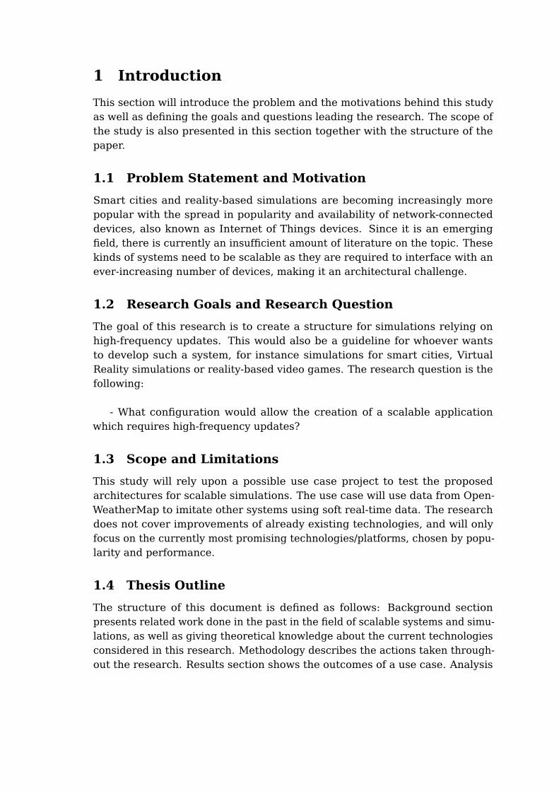
This section will introduce the problem and the motivations behind this studyas well as defining the goals and questions leading the research. The scope ofthe study is also presented in this section together with the structure of thepaper.

1.1 Problem Statement and Motivation

Smart cities and reality-based simulations are becoming increasingly morepopular with the spread in popularity and availability of network-connecteddevices, also known as Internet of Things devices. Since it is an emergingfield, there is currently an insufficient amount of literature on the topic. Thesekinds of systems need to be scalable as they are required to interface with anever-increasing number of devices, making it an architectural challenge.

1.2 Research Goals and Research Question

The goal of this research is to create a structure for simulations relying onhigh-frequency updates. This would also be a guideline for whoever wantsto develop such a system, for instance simulations for smart cities, VirtualReality simulations or reality-based video games. The research question is thefollowing:

- What configuration would allow the creation of a scalable applicationwhich requires high-frequency updates?

1.3 Scope and Limitations

This study will rely upon a possible use case project to test the proposedarchitectures for scalable simulations. The use case will use data from Open-WeatherMap to imitate other systems using soft real-time data. The researchdoes not cover improvements of already existing technologies, and will onlyfocus on the currently most promising technologies/platforms, chosen by popu-larity and performance.

1.4 Thesis Outline

The structure of this document is defined as follows: Background sectionpresents related work done in the past in the field of scalable systems and simu-lations, as well as giving theoretical knowledge about the current technologiesconsidered in this research. Methodology describes the actions taken through-out the research. Results section shows the outcomes of a use case. Analysis

2

and Discussion section assesses the performance of the use case project andattempts to extrapolate the data for other scenarios. In Conclusions and FutureWork, the study is summarized and connected to the field as a whole, discussingthe possible continuations of this project.

3

2 Background

This section will focus on the background for this study, providing notions andinformation for a better understanding of the topic.

2.1 Definitions

2.1.1 Scalable Systems

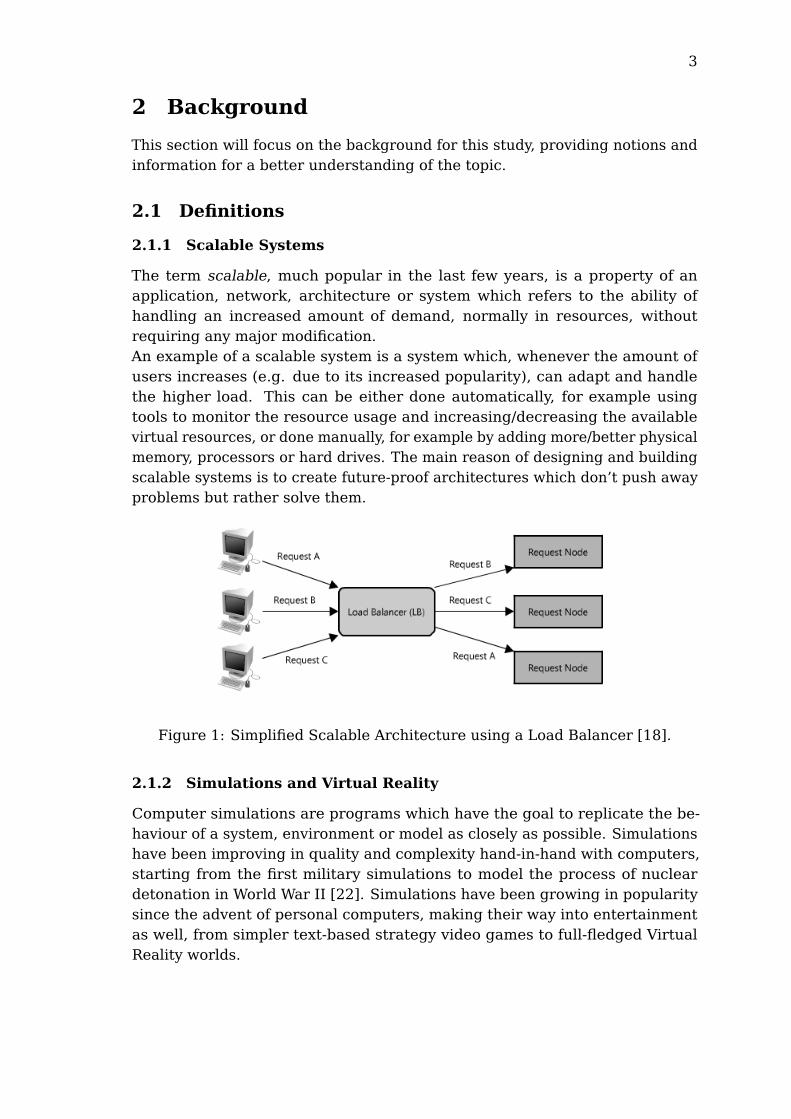
The term scalable, much popular in the last few years, is a property of anapplication, network, architecture or system which refers to the ability ofhandling an increased amount of demand, normally in resources, withoutrequiring any major modification.An example of a scalable system is a system which, whenever the amount ofusers increases (e.g. due to its increased popularity), can adapt and handlethe higher load. This can be either done automatically, for example usingtools to monitor the resource usage and increasing/decreasing the availablevirtual resources, or done manually, for example by adding more/better physicalmemory, processors or hard drives. The main reason of designing and buildingscalable systems is to create future-proof architectures which don’t push awayproblems but rather solve them.

Figure 1: Simplified Scalable Architecture using a Load Balancer [18].

2.1.2 Simulations and Virtual Reality

Computer simulations are programs which have the goal to replicate the be-haviour of a system, environment or model as closely as possible. Simulationshave been improving in quality and complexity hand-in-hand with computers,starting from the first military simulations to model the process of nucleardetonation in World War II [22]. Simulations have been growing in popularitysince the advent of personal computers, making their way into entertainmentas well, from simpler text-based strategy video games to full-fledged VirtualReality worlds.

4

Virtual Reality (often shortened as VR) can be defined as "the use of com-puter technology to create the effect of an interactive three-dimensional worldin which the objects have a sense of spatial presence" [1]. A defining character-istic of VR is the feeling of being immersed in a 3D environment. The illusionof immersion is usually created through Head-Mounted Displays (HMD’s) wornby the users, although other methods are available [2]. The first models HMD’swere being researched at NASA already back in 1986 [3]. Nowadays, more andmore HMD’s, such as the Oculus Rift and the HTC Vive, are being developed tomake this technology more widely available.

Real-time simulations, which are simulations making use of real-time data,are a type of simulation which have a possibility to become extremely prominentand popular in the future with the spread and improvement of affordable real-time IoT devices. With the use of sensors in critical areas (e.g. cities, forests,oceans, etc.), these simulations could make use of real-time information tosimulate and forecast the evolution of emergencies in order to help rescuesreact in a proper and safe manner [21]. This type of simulation would requirea constant, stable, up-to-date and high-frequency stream of data in order tomaintain a high fidelity simulation and forecast.

2.1.3 Virtualization

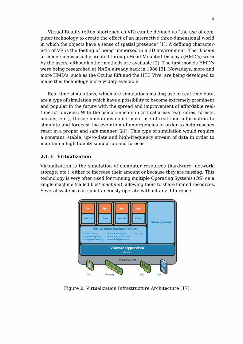
Virtualization is the simulation of computer resources (hardware, network,storage, etc.), either to increase their amount or because they are missing. Thistechnology is very often used for running multiple Operating Systems (OS) on asingle machine (called host machine), allowing them to share limited resources.Several systems can simultaneously operate without any difference.

Figure 2: Virtualization Infrastructure Architecture [17].

5

2.1.4 Docker

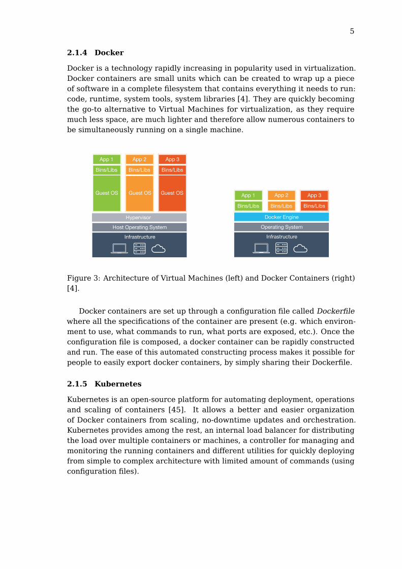
Docker is a technology rapidly increasing in popularity used in virtualization.Docker containers are small units which can be created to wrap up a pieceof software in a complete filesystem that contains everything it needs to run:code, runtime, system tools, system libraries [4]. They are quickly becomingthe go-to alternative to Virtual Machines for virtualization, as they requiremuch less space, are much lighter and therefore allow numerous containers tobe simultaneously running on a single machine.

Figure 3: Architecture of Virtual Machines (left) and Docker Containers (right)[4].

Docker containers are set up through a configuration file called Dockerfilewhere all the specifications of the container are present (e.g. which environ-ment to use, what commands to run, what ports are exposed, etc.). Once theconfiguration file is composed, a docker container can be rapidly constructedand run. The ease of this automated constructing process makes it possible forpeople to easily export docker containers, by simply sharing their Dockerfile.

2.1.5 Kubernetes

Kubernetes is an open-source platform for automating deployment, operationsand scaling of containers [45]. It allows a better and easier organizationof Docker containers from scaling, no-downtime updates and orchestration.Kubernetes provides among the rest, an internal load balancer for distributingthe load over multiple containers or machines, a controller for managing andmonitoring the running containers and different utilities for quickly deployingfrom simple to complex architecture with limited amount of commands (usingconfiguration files).

6

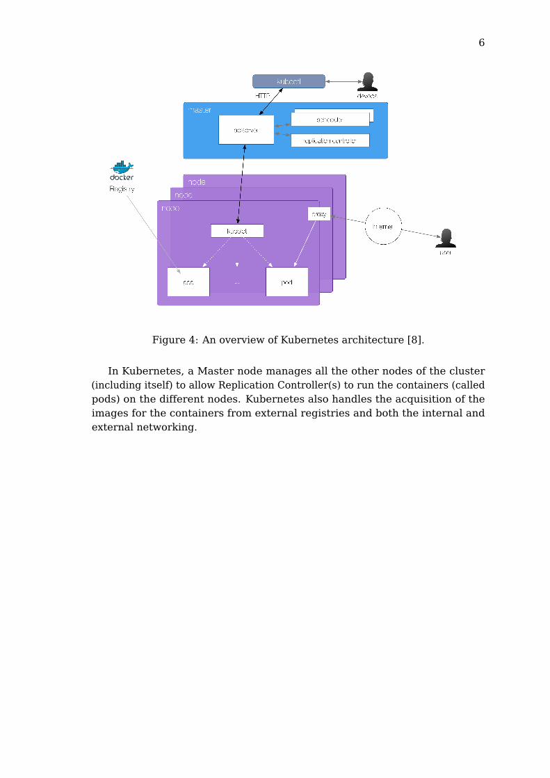
Figure 4: An overview of Kubernetes architecture [8].

In Kubernetes, a Master node manages all the other nodes of the cluster(including itself) to allow Replication Controller(s) to run the containers (calledpods) on the different nodes. Kubernetes also handles the acquisition of theimages for the containers from external registries and both the internal andexternal networking.

7

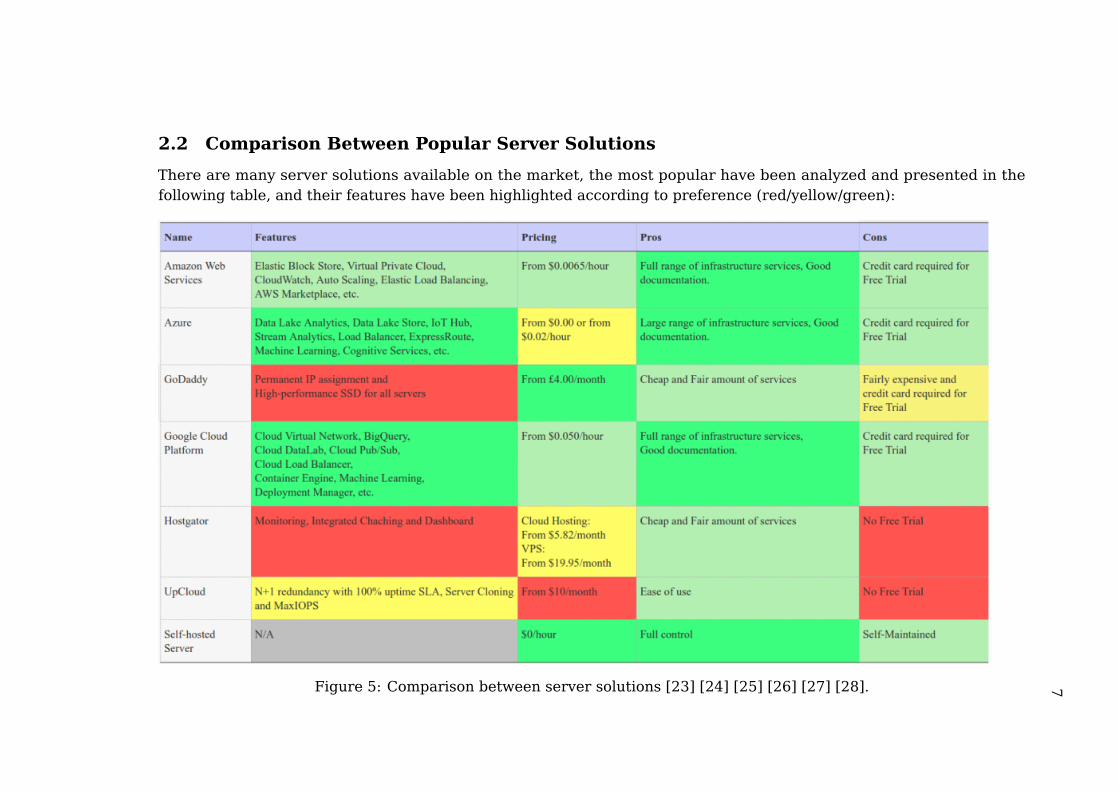
2.2 Comparison Between Popular Server Solutions

There are many server solutions available on the market, the most popular have been analyzed and presented in thefollowing table, and their features have been highlighted according to preference (red/yellow/green):

Figure 5: Comparison between server solutions [23] [24] [25] [26] [27] [28].

8

2.2.0.1 Amazon Web Services

Amazon Web Services (AWS) is a collection of cloud computing services byAmazon which includes a wide large variety of products, from robust hostingand scalable databases to APIs for Human Intelligence Tasks. In the selection,Amazon also has a container manager, EC2 Container Service, for creatingscalable architecture based on Docker containers [7].

2.2.0.2 Google Cloud Platform

Google Cloud Platform (GCP) is a cloud computing platform by Google whichprovides developer products, from hosting to container management and ma-chine learning [5].Among the available products, GCP offers Container Engine, a cluster man-ager and orchestration tool, based on Kubernetes, used for creating scalablearchitectures based on Docker containers [6].

2.2.0.3 Conclusions

Among the server solutions analyzed, both Google Cloud Platform and MicrosoftAzure provide a huge variety of services, from basic infrastructure ones tomachine learning, vision, speech, IoT and big data tools. Amazon Web Services,while being one of the most prominent players in the market of cloud platformswith high-quality infrastructures, seemed to lack the complexity and varietyof tools provided by Google and Microsoft. UpCloud, focusing mainly in cloudhosting, seemed to provide a fair and easy to use service with redundancy andpromises of 100% uptime.GoDaddy and Hostgator, mainly popular as web hosting providers, providedjust basic services for a server, without having as much as depth as the biggercompetitors.Most of them had a free trial available, except for UpCloud and Hostgator, andthey all required to register with a credit card right from the beginning.Since each vendor has their own type of business model, some billing certainservices per minute, per hour and some per month, the pricing shows thecheapest available options for each vendor.

The available server platforms available on the market have then beencompared to a self-hosted server, another very popular server solution.Given that having full and complete control over the system under test is theone of the most important aspects of an experiment, the self-hosted serverhas been chosen over the other options. All the other solutions provided veryinteresting and useful services for businesses but which are not necessary forthis study, especially because they require a big commitment to access them.Another reason is that the study will focus on pushing the limits of the server

9

in both requests and resources used, which on the other platforms might incuradditional fees.

2.3 Related Work

The research of similar projects and papers was used to acquire further knowl-edge on the topic of the study as well as to understand methodologies and tech-niques employed by other colleagues in the field. Related work has been foundby searching in the following databases: IEEE Xplore [9] and Essays.se [10].To find research in the field of virtual reality architectures, scalable architec-tures or scalable simulations that can be helpful for this study, the keywordsbelow have been used:

• Scalable architecture

• Simulation

• Kubernetes

• Dockers

Out of this search, around 40 relevant results have been found. This numberhas been reduced down to 10, by eliminating work that is not related to thefocus of the study. These elimination includes the studies focusing purelyon software architectures, not going into details regarding the networkingplatform used.

According to these findings, there has not been any study testing the per-formances of a server deployed standalone, on different dockers in paralleland on Kubernetes pods, with the focus on high-frequency requests from thesame client. On the other hand, there were 5 papers providing information andinsights useful for this study.

Prof. Ann Mary Joy [11] showed in her paper the comparison betweenVirtual Machines and Linux Containers (LXC). The study focused on the perfor-mance and scalability of the two server solutions with load testing. In her study,the LXC’s had much better results in both in terms of server performance andscalability. Although mentioned, Kubernetes was not individually tested andcompared to the other configurations.

G. Vigueras, M. Lozano et al. [12] worked on a scalable architecture forcrowd simulation, focusing on the internal software architecture of their solu-tion and providing benchmarks for the improved response times. The papershow that using a parallel action server can already lead to increase serverperformances.

10

Claus Pahl [13], in his article about containerization, presented containersand their differences compared to Virtual Machines. Dockers are taken as ex-ample of Linux Containers and described in details, together with Kubernetes.The article introduced some concepts in-depth but did not provide any dataregarding the performance of neither Docker container nor of Virtual Machines.

Azzedine Boukerche, Ming Zhang et al. [14] worked on an adaptive vir-tual simulation and real-time emergency response system, basing it on P2Pnetworks and JXTA [15]. Their paper focused on the system design from thesoftware point of view. They comment that attempting to use and benchmarktheir solution in a large-scale interconnected cluster could be done as futurework. The results from this current study could be also useful for their work.

David Bernstein [16] talked in his article about LXC’s, Docker Containersand Kubernetes, going into details on their high-level architecture, connectingit to standard Virtual Machines. The article, being purely descriptive, did notinclude any benchmark or performance comparison between the different typesof containers.

11

3 Methodology

This section will provide a guideline of how the study has been conducted,defining the research methodologies and their application.

3.1 Definitions

3.1.1 Experimental Research

Experimental Research is a scientific approach to research a subject by manip-ulating, controlling and measuring variables in an experiment [20].This can be useful to determine the effect of certain parameters or settings byevaluating their effect on the tested architecture.

3.2 Outline of Experiment

3.2.1 System Architecture

In order to effectively compare different architecture solutions, as described inthe Experimental Research approach, only the components under test shouldbe variable, the rest must remain unaltered.With this in mind, the following system architecture has been designed, whereonly the internal architecture of the server changes whilst performing thedifferent experiments:

Figure 6: General architecture of the systems under test.

12

The architecture of the system can be divided into 3 main parts: client,server and database.

3.2.2 Client

On the client is where the simulations are supposed to be running. In thisexperiment, the client(s) requesting updated data from the server will berepresented by a single computer making different amounts of requests perminute. This would put different levels of stress on the architectures undertest, showing their resilience, scalability and performance.For this experiment, 2 types of stress testing tools will be used: a home-madeimplementation and an already made tool.

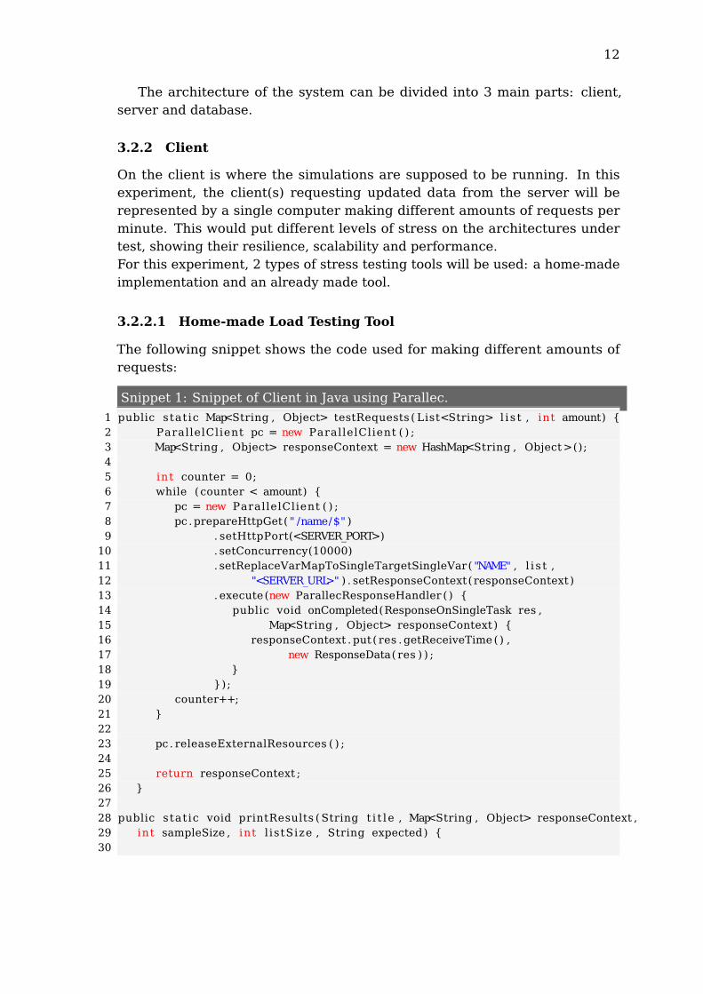
3.2.2.1 Home-made Load Testing Tool

The following snippet shows the code used for making different amounts ofrequests:

Snippet 1: Snippet of Client in Java using Parallec.

1 public static Map<String , Object> testRequests ( List<String> l i s t , int amount) {2 ParallelClient pc = new ParallelClient ( ) ;3 Map<String , Object> responseContext = new HashMap<String , Object>();45 int counter = 0;6 while (counter < amount) {7 pc = new ParallelClient ( ) ;8 pc .prepareHttpGet( " /name/$" )9 . setHttpPort(<SERVER_PORT>)

10 . setConcurrency(10000)11 . setReplaceVarMapToSingleTargetSingleVar( "NAME" , l i s t ,12 "<SERVER_URL>" ) . setResponseContext(responseContext )13 . execute(new ParallecResponseHandler ( ) {14 public void onCompleted(ResponseOnSingleTask res ,15 Map<String , Object> responseContext ) {16 responseContext . put ( res . getReceiveTime ( ) ,17 new ResponseData( res ) ) ;18 }19 });20 counter++;21 }2223 pc . releaseExternalResources ( ) ;2425 return responseContext ;26 }2728 public static void printResults ( String t i t le , Map<String , Object> responseContext ,29 int sampleSize , int l istSize , String expected) {30

13

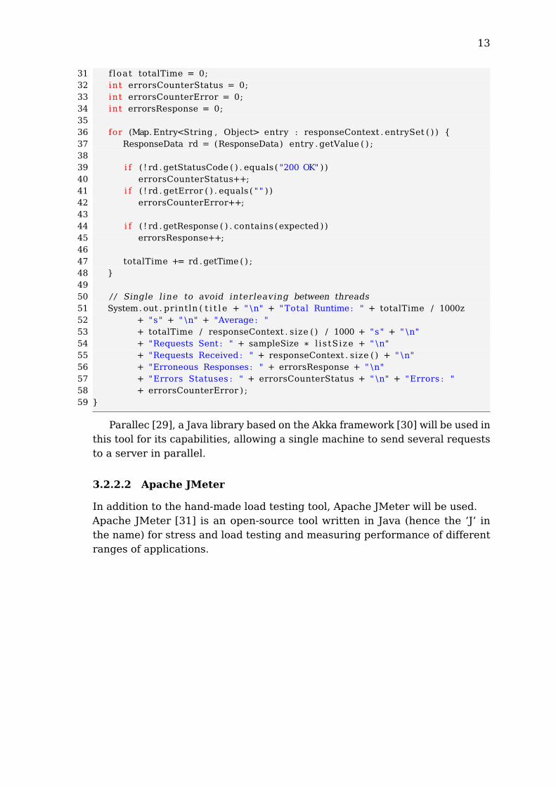
31 float totalTime = 0;32 int errorsCounterStatus = 0;33 int errorsCounterError = 0;34 int errorsResponse = 0;3536 for (Map. Entry<String , Object> entry : responseContext . entrySet ( ) ) {37 ResponseData rd = (ResponseData) entry . getValue ( ) ;3839 i f ( ! rd . getStatusCode ( ) . equals ( "200 OK" ) )40 errorsCounterStatus++;41 i f ( ! rd . getError ( ) . equals ( " " ) )42 errorsCounterError++;4344 i f ( ! rd .getResponse ( ) . contains (expected ) )45 errorsResponse++;4647 totalTime += rd .getTime ( ) ;48 }4950 / / Single line to avoid interleaving between threads51 System. out . println ( t i t l e + " \n" + "Total Runtime: " + totalTime / 1000z52 + "s" + " \n" + "Average: "53 + totalTime / responseContext . size ( ) / 1000 + "s" + " \n"54 + "Requests Sent : " + sampleSize * l istSize + " \n"55 + "Requests Received : " + responseContext . size ( ) + " \n"56 + "Erroneous Responses : " + errorsResponse + " \n"57 + "Errors Statuses : " + errorsCounterStatus + " \n" + "Errors : "58 + errorsCounterError ) ;59 }

Parallec [29], a Java library based on the Akka framework [30] will be used inthis tool for its capabilities, allowing a single machine to send several requeststo a server in parallel.

3.2.2.2 Apache JMeter

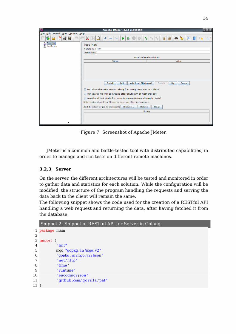
In addition to the hand-made load testing tool, Apache JMeter will be used.Apache JMeter [31] is an open-source tool written in Java (hence the ’J’ inthe name) for stress and load testing and measuring performance of differentranges of applications.

14

Figure 7: Screenshot of Apache JMeter.

JMeter is a common and battle-tested tool with distributed capabilities, inorder to manage and run tests on different remote machines.

3.2.3 Server

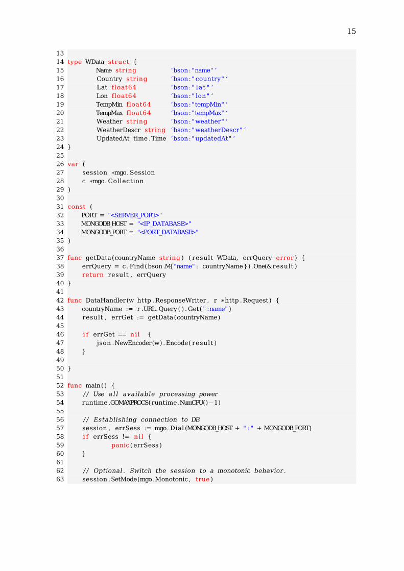
On the server, the different architectures will be tested and monitored in orderto gather data and statistics for each solution. While the configuration will bemodified, the structure of the program handling the requests and serving thedata back to the client will remain the same.The following snippet shows the code used for the creation of a RESTful APIhandling a web request and returning the data, after having fetched it fromthe database:

Snippet 2: Snippet of RESTful API for Server in Golang.

1 package main23 import (4 "fmt"5 mgo "gopkg. in /mgo.v2"6 "gopkg. in /mgo.v2/bson"7 "net / http"8 "time"9 "runtime"

10 "encoding / json"11 "github .com/ gori l la / pat"12 )

15

1314 type WData struct {15 Name string ‘bson:"name" ‘16 Country string ‘bson:" country" ‘17 Lat float64 ‘bson:" lat " ‘18 Lon float64 ‘bson:" lon" ‘19 TempMin float64 ‘bson:"tempMin" ‘20 TempMax float64 ‘bson:"tempMax" ‘21 Weather string ‘bson:"weather" ‘22 WeatherDescr string ‘bson:"weatherDescr" ‘23 UpdatedAt time .Time ‘bson:"updatedAt" ‘24 }2526 var (27 session *mgo. Session28 c *mgo. Collection29 )3031 const (32 PORT = "<SERVER_PORT>"33 MONGODB_HOST = "<IP_DATABASE>"34 MONGODB_PORT = "<PORT_DATABASE>"35 )3637 func getData(countryName string ) ( result WData, errQuery error ) {38 errQuery = c . Find(bson .M{"name" : countryName}).One(&result )39 return result , errQuery40 }4142 func DataHandler(w http .ResponseWriter , r *http .Request) {43 countryName := r .URL.Query ( ) . Get( " :name" )44 result , errGet := getData(countryName)4546 i f errGet == ni l {47 json .NewEncoder(w) .Encode( result )48 }4950 }5152 func main( ) {53 / / Use a l l available processing power54 runtime .GOMAXPROCS(runtime .NumCPU()−1)5556 / / Establishing connection to DB57 session , errSess := mgo. Dial (MONGODB_HOST + " : " + MONGODB_PORT)58 i f errSess != ni l {59 panic (errSess )60 }6162 / / Optional . Switch the session to a monotonic behavior .63 session .SetMode(mgo.Monotonic , true )

16

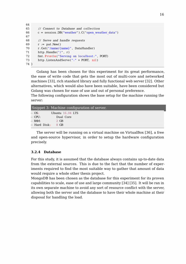
6465 / / Connect to Database and collection66 c = session .DB( "weather" ) .C( "open_weather_data" )6768 / / Serve and handle requests69 r := pat .New()70 r .Get( " /name/{name}" , DataHandler)71 http .Handle( " / " , r )72 fmt . Println ( "Serving on localhost : " , PORT)73 http . ListenAndServe( " : " + PORT, ni l )74 }

Golang has been chosen for this experiment for its great performance,the ease of write code that gets the most out of multi-core and networkedmachines [33], rich standard library and fully functional web server [32]. Otheralternatives, which would also have been suitable, have been considered butGolang was chosen for ease of use and out of personal preference.The following configuration shows the base setup for the machine running theserver:

Snippet 3: Machine configuration of server.

− OS: Ubuntu 16.04 LTS− CPU: Dual Core− RAM: 2 GB− Hard Disk : 8 GB

The server will be running on a virtual machine on VirtualBox [36], a freeand open-source hypervisor, in order to setup the hardware configurationprecisely.

3.2.4 Database

For this study, it is assumed that the database always contains up-to-date datafrom the external sources. This is due to the fact that the number of exper-iments required to find the most suitable way to gather that amount of datawould require a whole other thesis project.MongoDB has been chosen as the database for this experiment for its provencapabilities to scale, ease of use and large community [34] [35]. It will be ran inits own separate machine to avoid any sort of resource conflict with the server,allowing both the server and the database to have their whole machine at theirdisposal for handling the load.

17

The following configuration shows the base setup for the machine runningthe database:

Snippet 4: Machine configuration of database.

− OS: Ubuntu 16.04 LTS− CPU: Quad Core− RAM: 4 GB− Hard Disk : 4 GB

The database will also be running on a VM but a more powerful machine hasbeen assigned to it in order to decrease its chance of becoming the bottleneckof the system and thus invalidating some of the results of the experiment.

The data contained in the database will be from the daily bulk sample fromthe OpenWatherMap dataset, which contains weather information and forecastfrom over 200.000 cities [37]. The following snippet shows the structure of thedata contained in the sample:

Snippet 5: Sample of weather data from OpenWeatherMap.

{" city " : {

" id " : 519188,"name" : "Novinki" ,"country" : "RU" ,"coord" : {

" lon" : 37.666668," lat " : 55.683334

}},"time" : 1394864756,"data" : [

{"dt" : 1394787600,"temp" : {

"day" : 279.65,"min" : 275.12,"max" : 279.65,"night" : 275.12,"eve" : 276.44,"morn" : 279.65

},"pressure" : 989.79,"humidity" : 0,"weather" : [

{" id " : 500,"main" : "Rain" ,"description" : " l ight rain" ," icon" : "10dd"

}

18

] ,"speed" : 9.85,"deg" : 277,"clouds" : 76

}]

}

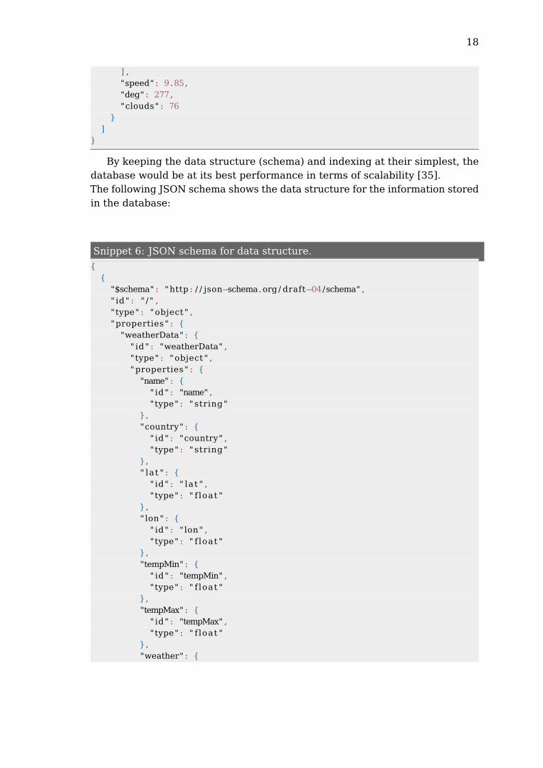
By keeping the data structure (schema) and indexing at their simplest, thedatabase would be at its best performance in terms of scalability [35].The following JSON schema shows the data structure for the information storedin the database:

Snippet 6: JSON schema for data structure.

{{

"$schema" : "http : / / json−schema. org / draft−04/schema" ," id " : " / " ,"type" : "object " ,"properties" : {

"weatherData" : {" id " : "weatherData" ,"type" : "object " ,"properties" : {

"name" : {" id " : "name" ,"type" : " string "

},"country" : {

" id " : "country" ,"type" : " string "

}," lat " : {

" id " : " lat " ,"type" : " f loat "

}," lon" : {

" id " : " lon" ,"type" : " f loat "

},"tempMin" : {

" id " : "tempMin" ,"type" : " f loat "

},"tempMax" : {

" id " : "tempMax" ,"type" : " f loat "

},"weather" : {

19

" id " : "weather" ,"type" : " string "

},"weatherDescr" : {

" id " : "weatherDescr" ,"type" : " string "

}}

},"required" : [

"name" ,"country" ," lat " ," lon" ,"tempMin" ,"tempMax" ,"weather" ,"weatherDescr"

]},"required" : [

"weatherData"]

}}

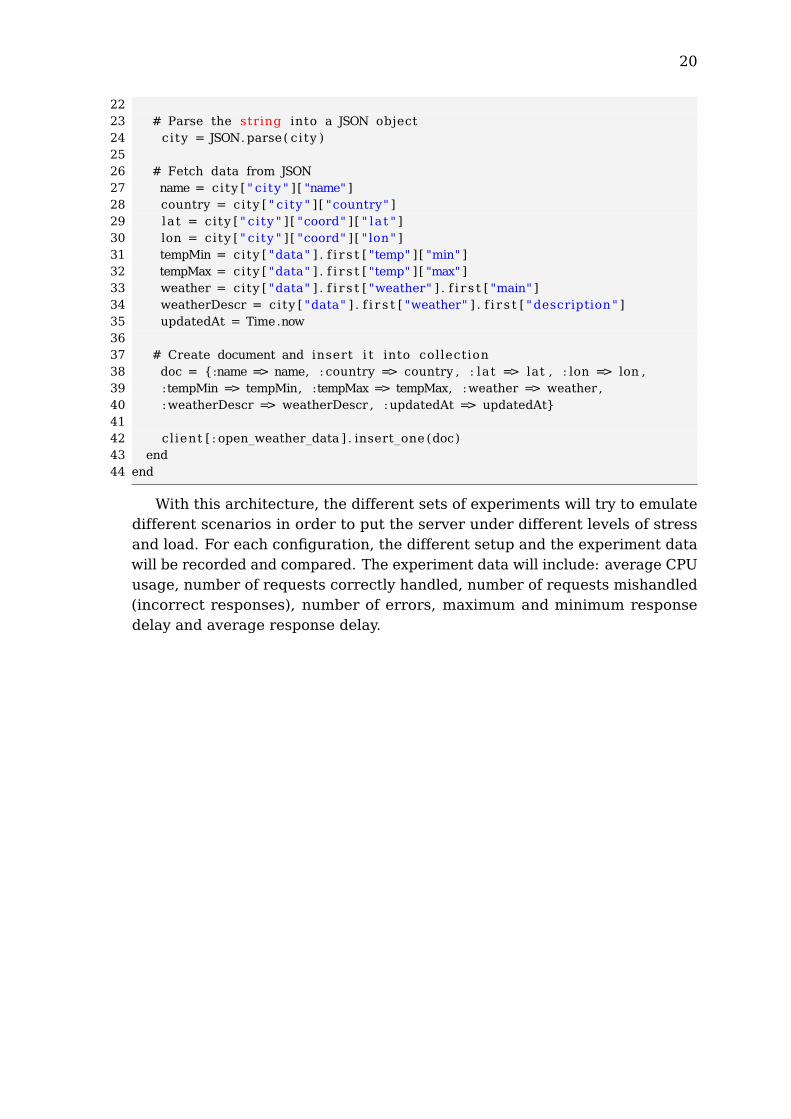
The following snippet shows the code used for importing of the weatherdata into the database:

Snippet 7: Snippet of weather importer in Ruby.

1 require ’ json ’2 require ’mongo’3 require ’pp ’45 include Mongo67 client = Mongo: : Client .new([ ’<IP_DATABASE>:<PORT_DATABASE>’ ] ,8 :database => ’weather ’ )9

10 # Erase a l l records from collection , i f any11 client [ : open_weather_data ] . drop1213 # Create new collection14 client [ : open_weather_data ] . create1516 # Read weather data f i l e17 f i l e = File . read( ’<FILENAME>.json ’ )18 cit ies = f i l e . sp l i t ( " \n" ) ;1920 cit ies .each do | city |21 begin

20

2223 # Parse the string into a JSON object24 city = JSON. parse( city )2526 # Fetch data from JSON27 name = city [ " city " ] [ "name" ]28 country = city [ " city " ] [ "country" ]29 lat = city [ " city " ] [ "coord" ] [ " lat " ]30 lon = city [ " city " ] [ "coord" ] [ " lon" ]31 tempMin = city [ "data" ] . f i r s t [ "temp" ] [ "min" ]32 tempMax = city [ "data" ] . f i r s t [ "temp" ] [ "max" ]33 weather = city [ "data" ] . f i r s t [ "weather" ] . f i r s t [ "main" ]34 weatherDescr = city [ "data" ] . f i r s t [ "weather" ] . f i r s t [ "description" ]35 updatedAt = Time.now3637 # Create document and insert i t into collection38 doc = {:name => name, : country => country , : lat => lat , : lon => lon ,39 :tempMin => tempMin, :tempMax => tempMax, :weather => weather ,40 :weatherDescr => weatherDescr , :updatedAt => updatedAt}4142 client [ : open_weather_data ] . insert_one (doc)43 end44 end

With this architecture, the different sets of experiments will try to emulatedifferent scenarios in order to put the server under different levels of stressand load. For each configuration, the different setup and the experiment datawill be recorded and compared. The experiment data will include: average CPUusage, number of requests correctly handled, number of requests mishandled(incorrect responses), number of errors, maximum and minimum responsedelay and average response delay.

21

3.3 Server Architectures Under Test

3.3.1 Standalone Server

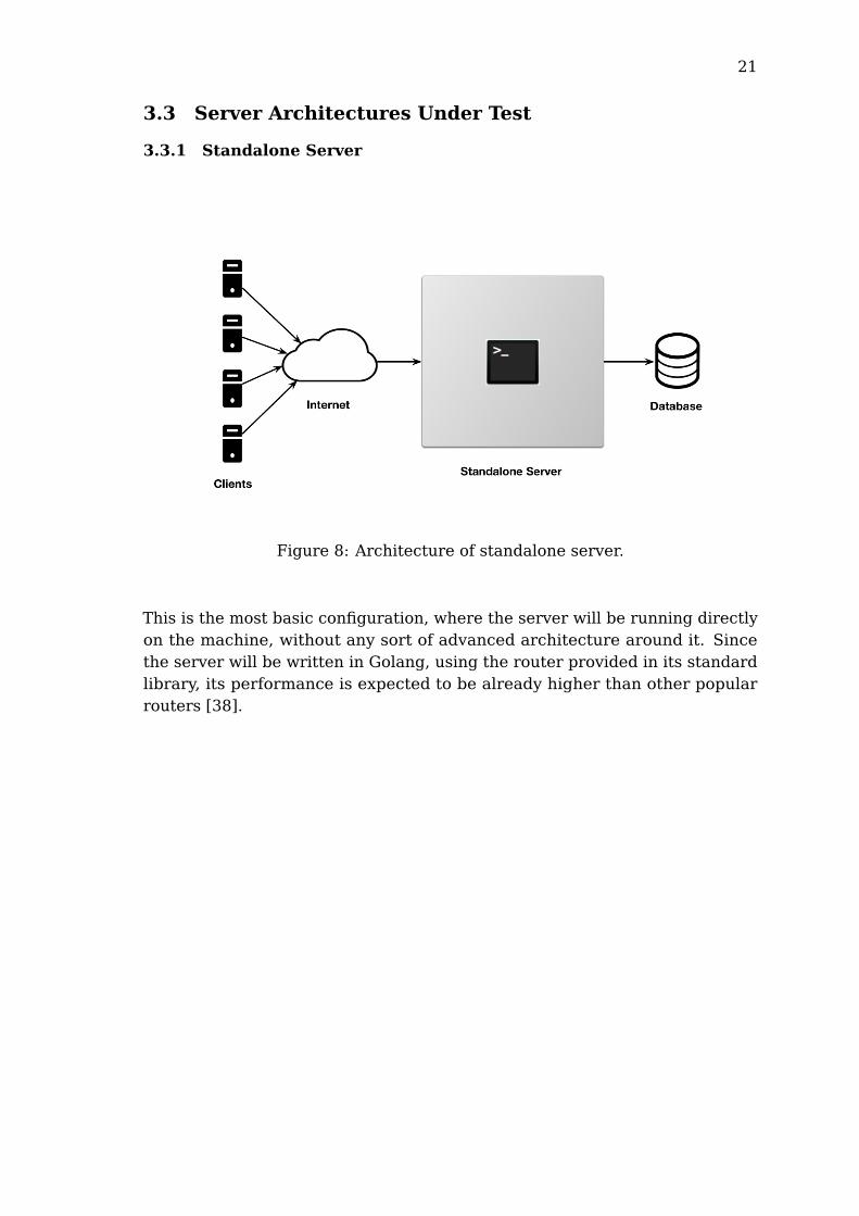
Figure 8: Architecture of standalone server.

This is the most basic configuration, where the server will be running directlyon the machine, without any sort of advanced architecture around it. Sincethe server will be written in Golang, using the router provided in its standardlibrary, its performance is expected to be already higher than other popularrouters [38].

22

3.3.2 Server on Docker

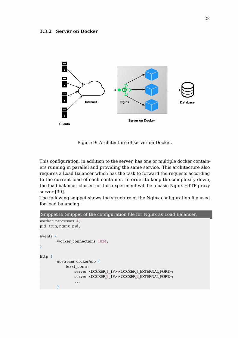
Figure 9: Architecture of server on Docker.

This configuration, in addition to the server, has one or multiple docker contain-ers running in parallel and providing the same service. This architecture alsorequires a Load Balancer which has the task to forward the requests accordingto the current load of each container. In order to keep the complexity down,the load balancer chosen for this experiment will be a basic Nginx HTTP proxyserver [39].The following snippet shows the structure of the Nginx configuration file usedfor load balancing:

Snippet 8: Snippet of the configuration file for Nginx as Load Balancer.

worker_processes 4;pid / run/ nginx . pid ;

events {worker_connections 1024;

}

http {upstream dockerApp {

least_conn ;server <DOCKER_1_IP>:<DOCKER_1_EXTERNAL_PORT>;server <DOCKER_2_IP>:<DOCKER_2_EXTERNAL_PORT>;. . .

}

23

server {l isten <EXTERNAL_PORT>;

location / {proxy_pass http : / / dockerApp;

}}

include servers / * ;}

3.3.3 Server on Kubernetes

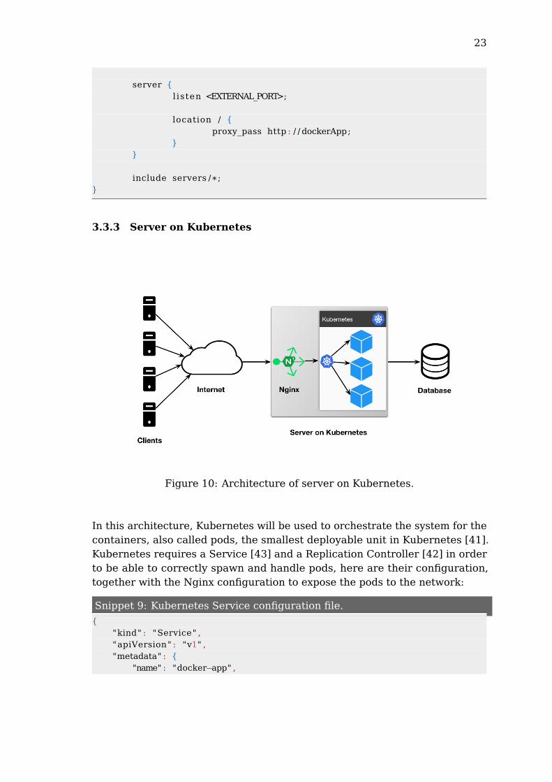
Figure 10: Architecture of server on Kubernetes.

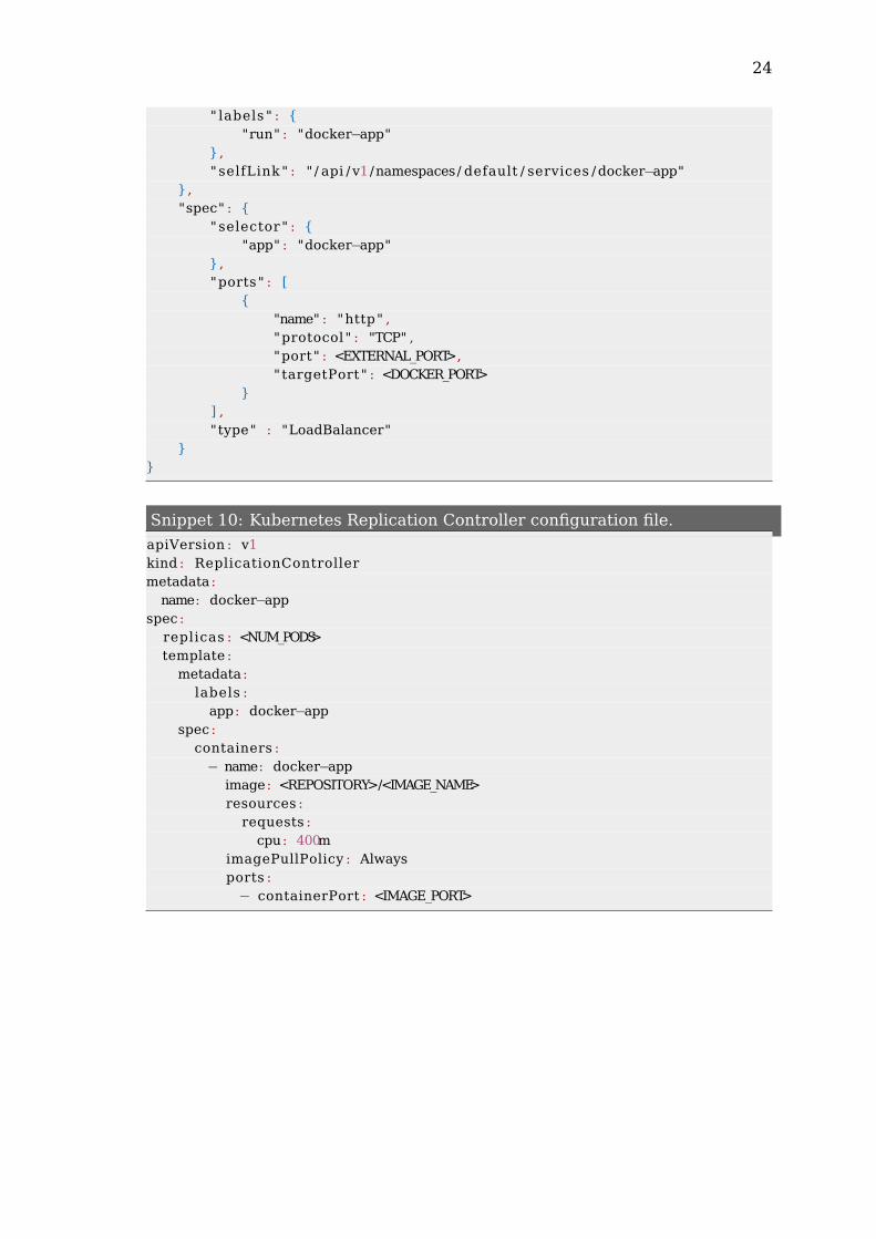
In this architecture, Kubernetes will be used to orchestrate the system for thecontainers, also called pods, the smallest deployable unit in Kubernetes [41].Kubernetes requires a Service [43] and a Replication Controller [42] in orderto be able to correctly spawn and handle pods, here are their configuration,together with the Nginx configuration to expose the pods to the network:

Snippet 9: Kubernetes Service configuration file.

{"kind" : "Service" ,"apiVersion" : "v1" ,"metadata" : {

"name" : "docker−app" ,

24

" labels " : {"run" : "docker−app"

}," selfLink " : " / api / v1/namespaces/ default / services /docker−app"

},"spec" : {

" selector " : {"app" : "docker−app"

},"ports" : [

{"name" : "http" ,"protocol" : "TCP" ,"port" : <EXTERNAL_PORT>," targetPort" : <DOCKER_PORT>

}] ,"type" : "LoadBalancer"

}}

Snippet 10: Kubernetes Replication Controller configuration file.

apiVersion : v1kind : ReplicationControllermetadata :

name: docker−appspec :

replicas : <NUM_PODS>template :

metadata :labels :

app: docker−appspec :

containers :− name: docker−app

image: <REPOSITORY>/<IMAGE_NAME>resources :

requests :cpu: 400m

imagePullPolicy : Alwaysports :

− containerPort : <IMAGE_PORT>

25

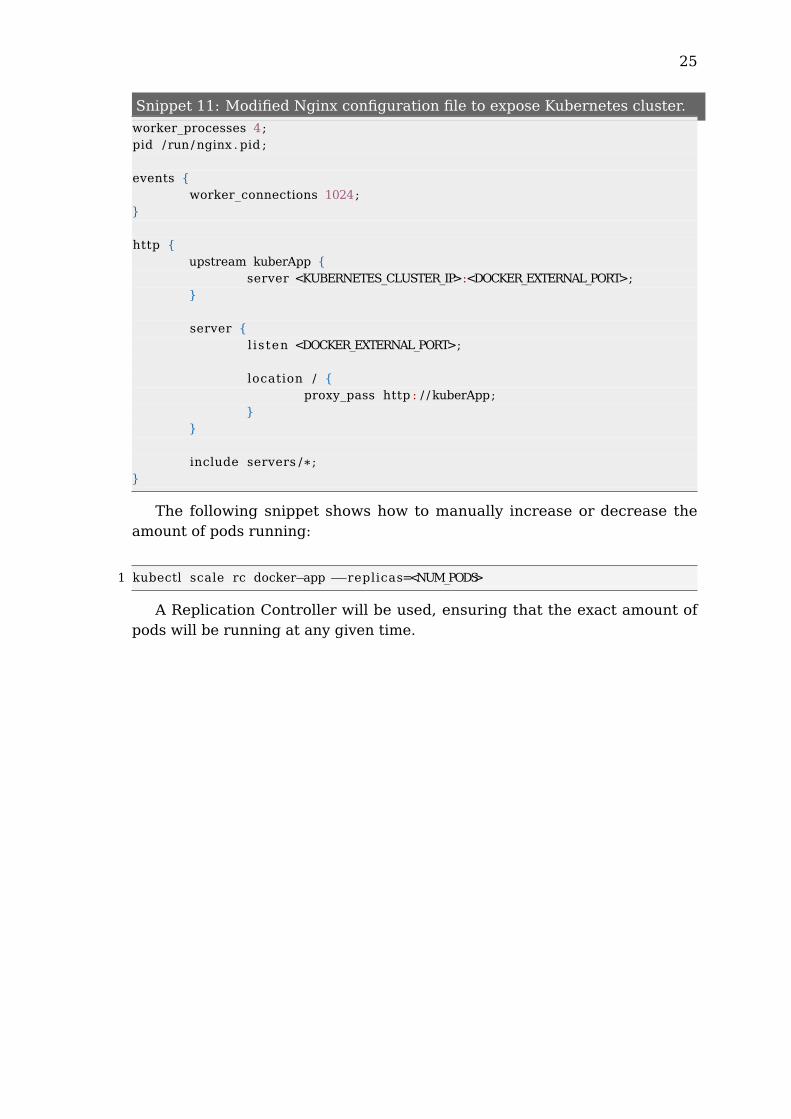
Snippet 11: Modified Nginx configuration file to expose Kubernetes cluster.

worker_processes 4;pid / run/ nginx . pid ;

events {worker_connections 1024;

}

http {upstream kuberApp {

server <KUBERNETES_CLUSTER_IP>:<DOCKER_EXTERNAL_PORT>;}

server {l isten <DOCKER_EXTERNAL_PORT>;

location / {proxy_pass http : / / kuberApp;

}}

include servers / * ;}

The following snippet shows how to manually increase or decrease theamount of pods running:

1 kubectl scale rc docker−app −−replicas=<NUM_PODS>

A Replication Controller will be used, ensuring that the exact amount ofpods will be running at any given time.

26

4 Results

In this section, experiment results are presented.

4.1 Experiments Output

After conducting the first few experiment, it has become clear that the hand-made tool would not suffice for properly load testing the different server con-figurations. This was mainly due to its extremely low amount of requests persecond. For this reason, Apache JMeter has been used as the unique loadtesting tool for the experiments.During each testing session raw data has been gathered and turned into ausable representations in order to make analysis and comparison betweenresults easier.

4.1.1 Aggregated Data

The Aggregated Data shows the combined result data giving a short summaryfor each of the experiments.The following table shows the structure of the aggregated data:

# Requests/Sec Mean Median Min Max Error %

Table 1: Aggregated data structure.

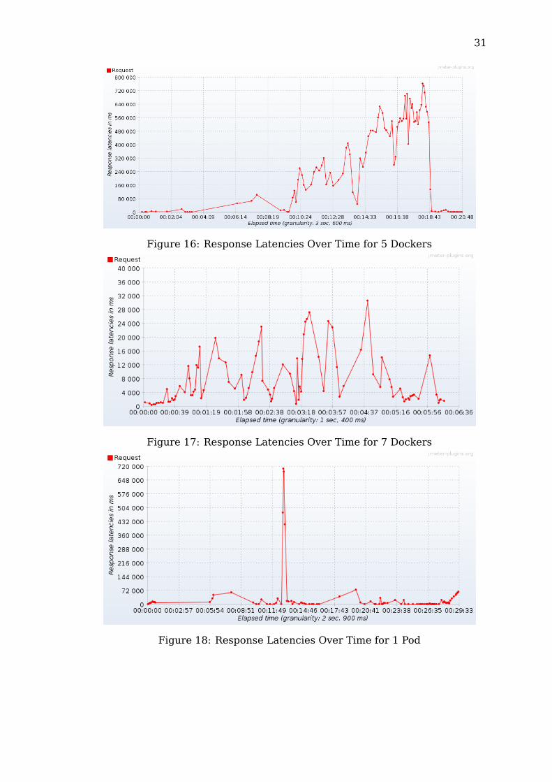
4.1.2 Response Latencies Over Time

Response Latencies Over Time is a graph showing the response latencies overthe duration of the experiment. It is useful to visualize the overall behaviourand eventual recovery capabilities of the server over time. Given the largeamount of data, the graph shows fewer but representative values.

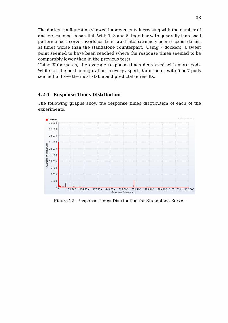
4.1.3 Response Times Distribution

Response Time Distribution is a graph showing the distribution of responselatencies. The distinguishing characteristic is that it can clearly show all theobserved values.

4.1.4 Response Codes per Second

Response Codes per Second is a graph showing the result of each request tothe server. This is a way to visualize the amount of good/bad responses from aspecific server configuration over time. Given the large amount of data, thegraph shows fewer but representative values.The following are the possible types of response:

27

• 200: HTTP Status code for OK, meaning: ’The request was fulfilled.’ [44]

• 500: HTTP Status code for Internal Error, meaning ’The server encoun-tered an unexpected condition which prevented it from fulfilling the re-quest. [44]’

• Non HTTP response code: org.apache.http.conn.HttpHostConnetException:Java error code, meaning ’The client could not connect to the server’

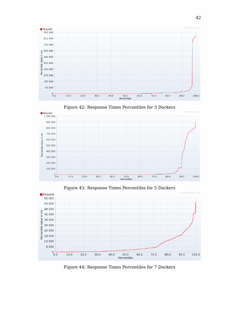
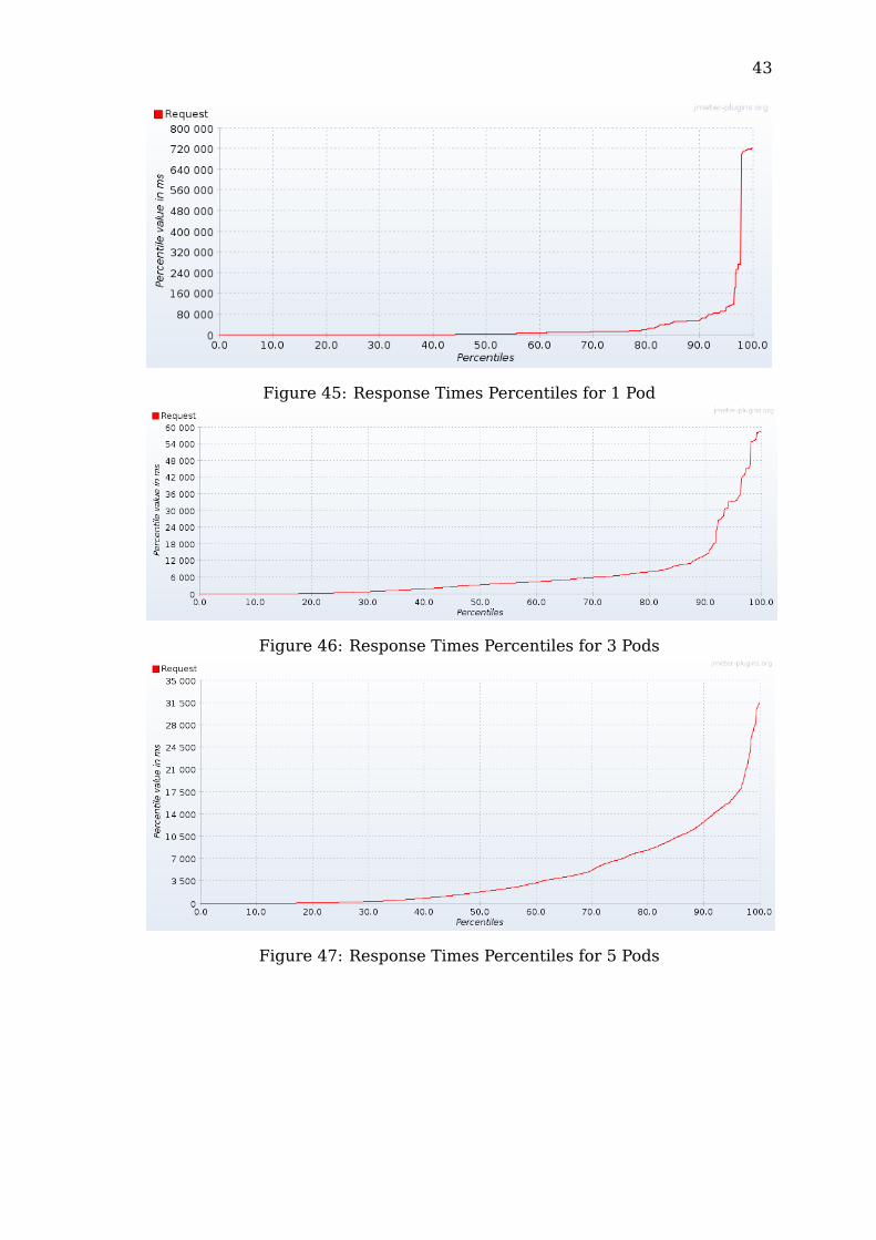
4.1.5 Response Times Percentiles

Response Times Percentiles is a graph which shows the response times bypercentage. This is a way to visualize the percentage of requests under aspecific threshold value.

28

4.2 Experiments Data

4.2.1 Aggregated Data

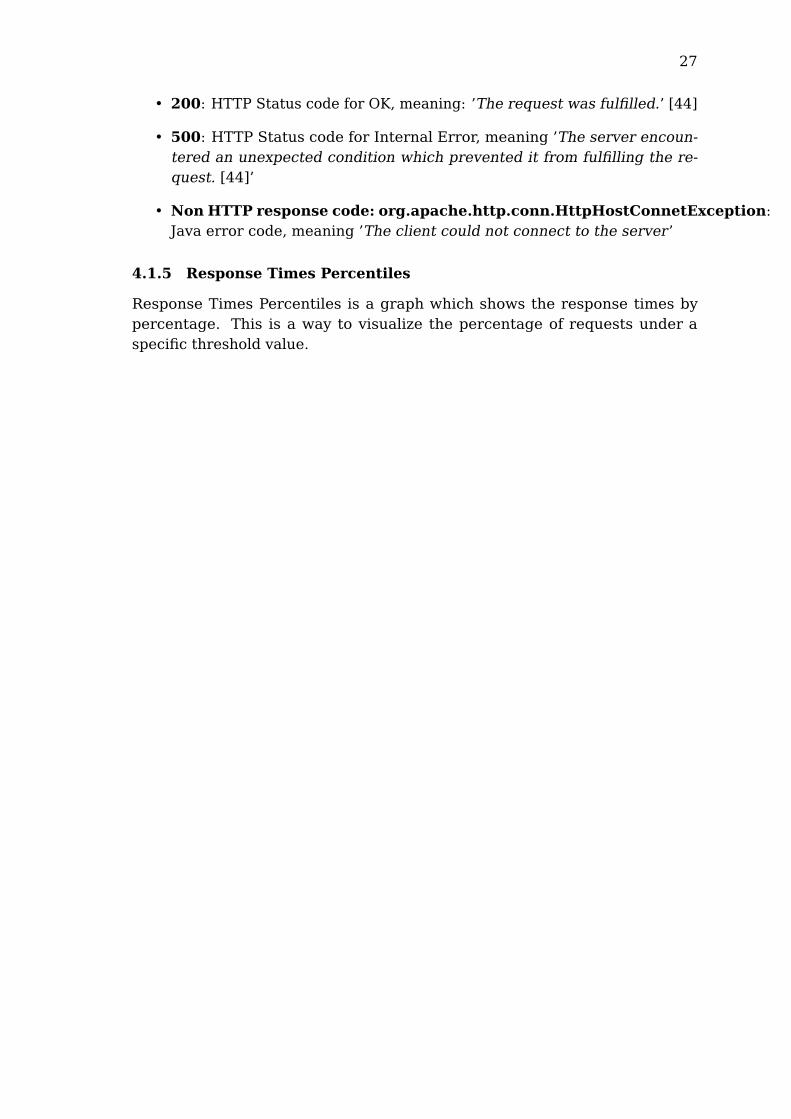
The following table contains the aggregated data showing the request fre-quency per second, response latencies, the delay between the request andreceiving a response, and the percentage of request errors for different serverconfigurations:

Requests/Sec Mean Median Min Max Error %

Standalone 178.9 139,512 64,271 7 1,123,452 34.34%

1 Docker 124.5 221,609 17,890 5 1,229,087 0.00%

3 Dockers 284.5 29,563 971 3 917,773 5.20%

5 Dockers 216.3 72,504 342 4 931,680 1.21%

7 Dockers 680.3 6,510 2,163 3 55,554 0.23%

1 Pod 152 33,021 4,537 1 723,982 5.16%

3 Pods 78.4 6,704 3,419 2 72,798 5.64%

5 Pods 176.7 4,468 1,852 1 37,570 19.77%

7 Pods 75.5 5,804 1,521 1 70,544 5.02%

Table 2: Aggregated results for different server configurations, latencies areexpressed in milliseconds.

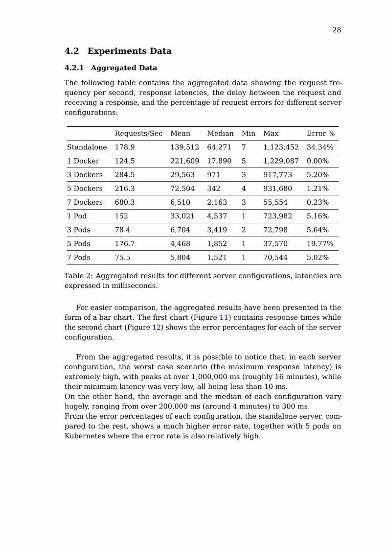
For easier comparison, the aggregated results have been presented in theform of a bar chart. The first chart (Figure 11) contains response times whilethe second chart (Figure 12) shows the error percentages for each of the serverconfiguration.

From the aggregated results, it is possible to notice that, in each serverconfiguration, the worst case scenario (the maximum response latency) isextremely high, with peaks at over 1,000,000 ms (roughly 16 minutes), whiletheir minimum latency was very low, all being less than 10 ms.On the other hand, the average and the median of each configuration varyhugely, ranging from over 200,000 ms (around 4 minutes) to 300 ms.From the error percentages of each configuration, the standalone server, com-pared to the rest, shows a much higher error rate, together with 5 pods onKubernetes where the error rate is also relatively high.

29

Figure 11: Chart of aggregated results.

Figure 12: Chart of error percentages.

30

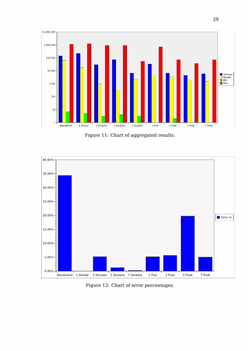
4.2.2 Response Latencies Over Time

Figure 13: Response Latencies Over Time for Standalone Server

Figure 14: Response Latencies Over Time for 1 Docker

Figure 15: Response Latencies Over Time for 3 Dockers

31

Figure 16: Response Latencies Over Time for 5 Dockers

Figure 17: Response Latencies Over Time for 7 Dockers

Figure 18: Response Latencies Over Time for 1 Pod

32

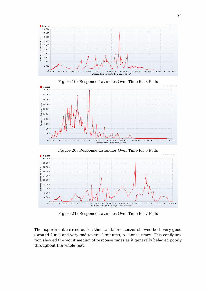
Figure 19: Response Latencies Over Time for 3 Pods

Figure 20: Response Latencies Over Time for 5 Pods

Figure 21: Response Latencies Over Time for 7 Pods

The experiment carried out on the standalone server showed both very good(around 2 ms) and very bad (over 12 minutes) response times. This configura-tion showed the worst median of response times as it generally behaved poorlythroughout the whole test.

33

The docker configuration showed improvements increasing with the number ofdockers running in parallel. With 1, 3 and 5, together with generally increasedperformances, server overloads translated into extremely poor response times,at times worse than the standalone counterpart. Using 7 dockers, a sweetpoint seemed to have been reached where the response times seemed to becomparably lower than in the previous tests.Using Kubernetes, the average response times decreased with more pods.While not the best configuration in every aspect, Kubernetes with 5 or 7 podsseemed to have the most stable and predictable results.

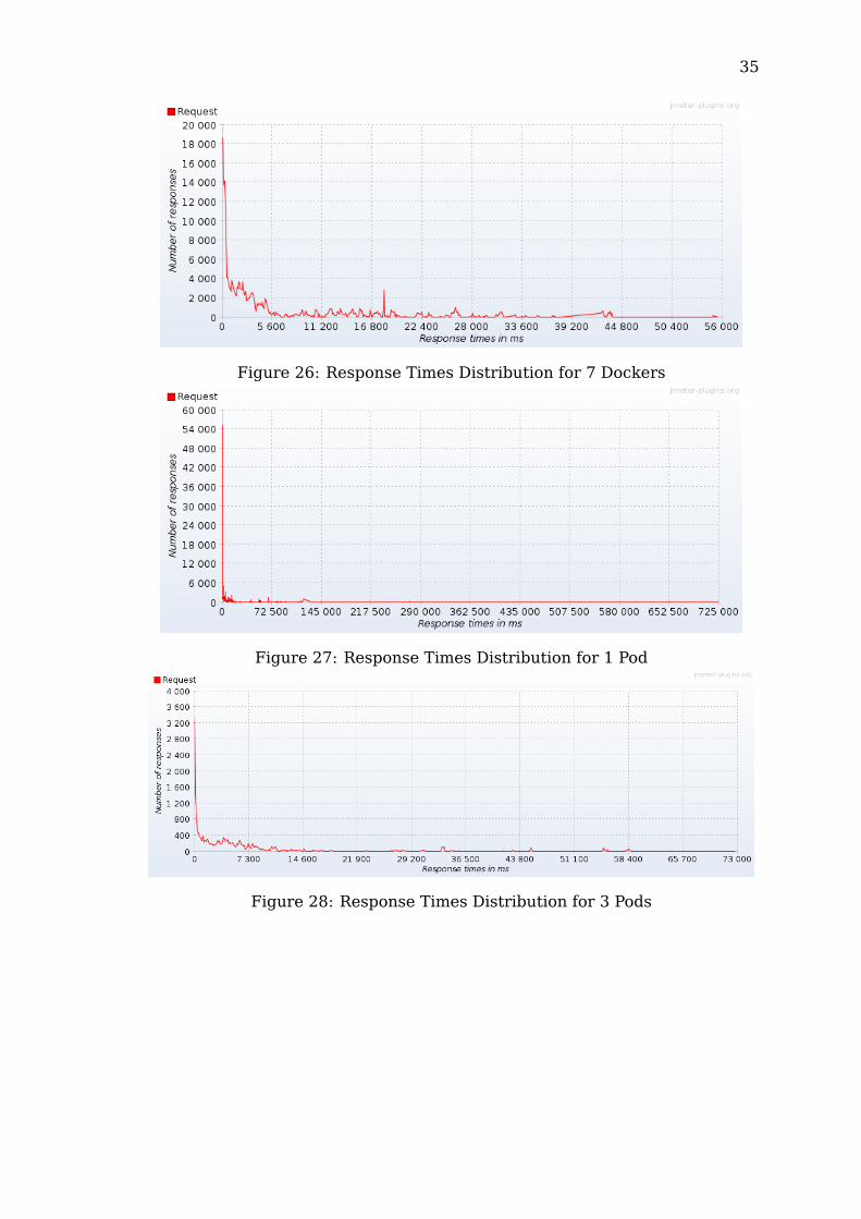
4.2.3 Response Times Distribution

The following graphs show the response times distribution of each of theexperiments:

Figure 22: Response Times Distribution for Standalone Server

34

Figure 23: Response Times Distribution for 1 Docker

Figure 24: Response Times Distribution for 3 Dockers

Figure 25: Response Times Distribution for 5 Dockers

35

Figure 26: Response Times Distribution for 7 Dockers

Figure 27: Response Times Distribution for 1 Pod

Figure 28: Response Times Distribution for 3 Pods

36

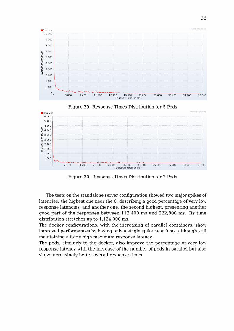
Figure 29: Response Times Distribution for 5 Pods

Figure 30: Response Times Distribution for 7 Pods

The tests on the standalone server configuration showed two major spikes oflatencies: the highest one near the 0, describing a good percentage of very lowresponse latencies, and another one, the second highest, presenting anothergood part of the responses between 112,400 ms and 222,800 ms. Its timedistribution stretches up to 1,124,000 ms.The docker configurations, with the increasing of parallel containers, showimproved performances by having only a single spike near 0 ms, although stillmaintaining a fairly high maximum response latency.The pods, similarly to the docker, also improve the percentage of very lowresponse latency with the increase of the number of pods in parallel but alsoshow increasingly better overall response times.

37

4.2.4 Response Codes per Second

The following graphs show the response codes per second of each of theexperiments:

Figure 31: Response Codes per Second for Standalone Server

Figure 32: Response Codes per Second for 1 Docker

38

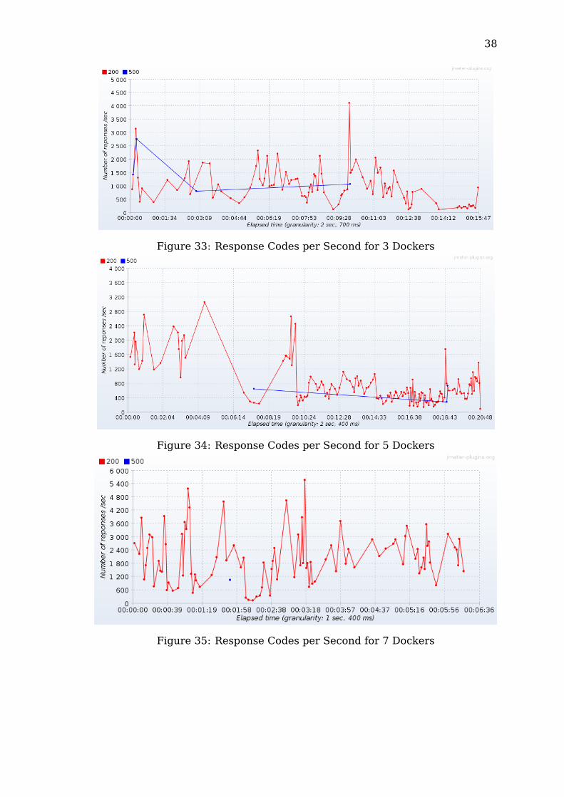
Figure 33: Response Codes per Second for 3 Dockers

Figure 34: Response Codes per Second for 5 Dockers

Figure 35: Response Codes per Second for 7 Dockers

39

Figure 36: Response Codes per Second for 1 Pod

Figure 37: Response Codes per Second for 3 Pods

Figure 38: Response Codes per Second for 5 Pods

40

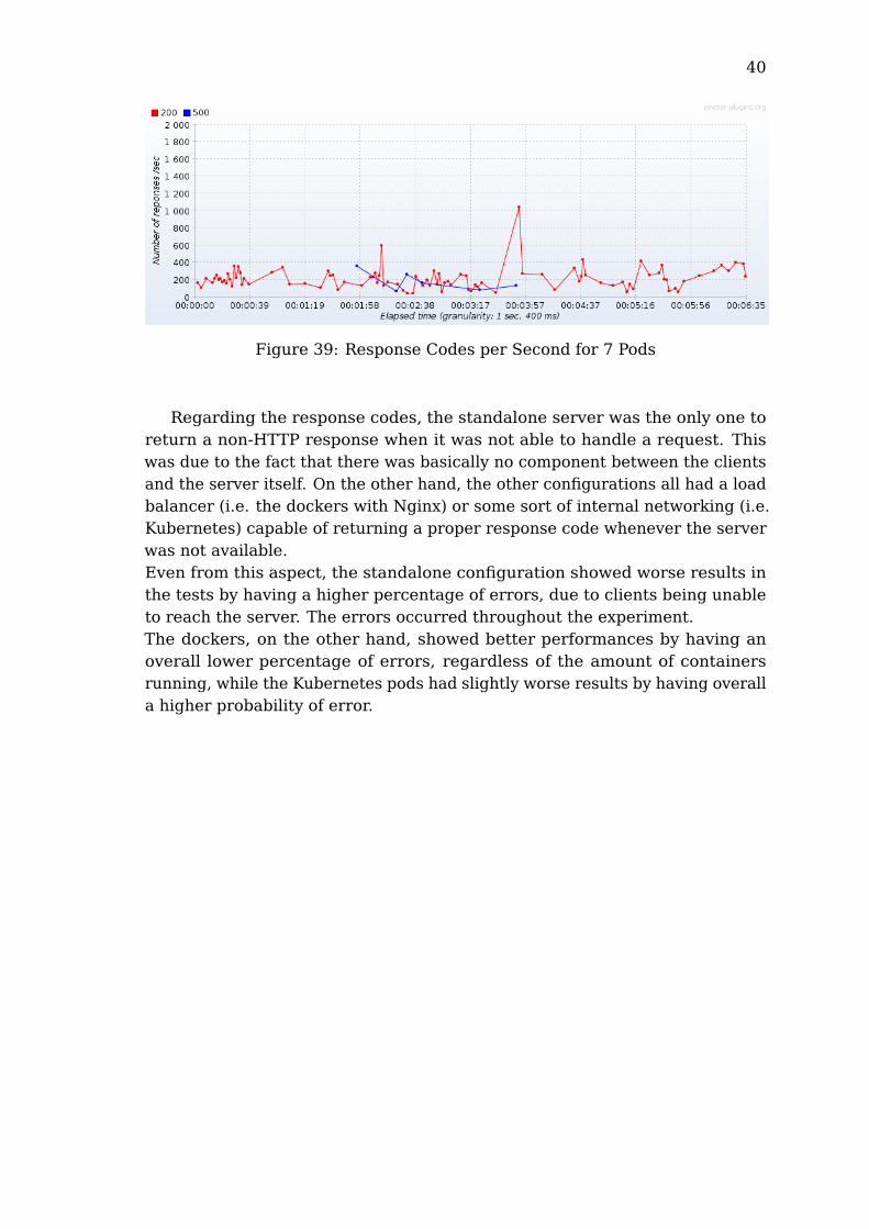
Figure 39: Response Codes per Second for 7 Pods

Regarding the response codes, the standalone server was the only one toreturn a non-HTTP response when it was not able to handle a request. Thiswas due to the fact that there was basically no component between the clientsand the server itself. On the other hand, the other configurations all had a loadbalancer (i.e. the dockers with Nginx) or some sort of internal networking (i.e.Kubernetes) capable of returning a proper response code whenever the serverwas not available.Even from this aspect, the standalone configuration showed worse results inthe tests by having a higher percentage of errors, due to clients being unableto reach the server. The errors occurred throughout the experiment.The dockers, on the other hand, showed better performances by having anoverall lower percentage of errors, regardless of the amount of containersrunning, while the Kubernetes pods had slightly worse results by having overalla higher probability of error.

41

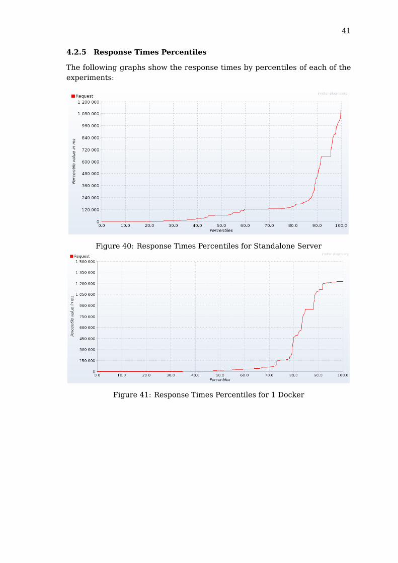
4.2.5 Response Times Percentiles

The following graphs show the response times by percentiles of each of theexperiments:

Figure 40: Response Times Percentiles for Standalone Server

Figure 41: Response Times Percentiles for 1 Docker

42

Figure 42: Response Times Percentiles for 3 Dockers

Figure 43: Response Times Percentiles for 5 Dockers

Figure 44: Response Times Percentiles for 7 Dockers

43

Figure 45: Response Times Percentiles for 1 Pod

Figure 46: Response Times Percentiles for 3 Pods

Figure 47: Response Times Percentiles for 5 Pods

44

Figure 48: Response Times Percentiles for 7 Pods

From the results, half of the requests send to the standalone server wereeach handled within 60,000 ms (1 minute). During the test, the response timestook a first peak between 85% and 90% and a final one from 95%, showing ahuge increase of the response times.The dockers, while being able to generally handle the requests much morequickly, also showed a very high peak, from 80% to 90% of its responses. Theconfiguration with 7 dockers overall performed better than the first 50% partof the standalone server.The pods while initially performing quite poorly, their performance started tostabilize to the point of not having any peak but rather a constantly increasingcurve. Even if apparently similar, compared to the rest, the graphs show thatthe pods had, in overall, much lower response times.

45

5 Analysis and Discussion

By comparing the different server configuration, focusing on different aspects,the tests allowed to gather data and insights regarding the performance trendsof each server configuration. The standalone server almost always behavedpoorly, even by comparing it only to a single instance of a Docker container orKubernetes pod.Both the Docker and the Kubernetes configurations generally showed an in-crease in performance in relation to the number of containers (or pods) runningin parallel. The higher the number of service providers simultaneously running,the higher the amount of requests handled and their response speed.In certain cases some aspects of the tests showed data going against the perfor-mance trends, that can be connected to the variability of independent factors,such as the speed/quality of the network between the clients and the server.The error rates of the different configurations are also probably connected tothe different handling of incoming traffic (e.g. the requests), with the stan-dalone having a very minimal one directly from the Operating System itself,the docker containers relying on Nginx and the internal docker manager andKubernetes using its more advanced networking [46]. This would signify thateven having a simple network interface could already decrease the error ratequite dramatically, as seen in the single Docker configuration.The study by Prof. Ann Mary Joy [11], which compared Linux Containers(LXC), more specifically Docker containers, and Virtual Machines, also showedDockers to have better performances and better scalability features than astandalone server. For the load testing in the study, Apache JMeter was alsoused to send as many request as possible to the system under test.

46

6 Conclusions and Future Work

Whenever designing a scalable architecture, it is important to choose the righttools. This study, focusing on an architecture needing high-frequency update re-quests, such as real-time simulations or emergency response systems, showedthat deploying containers can be a good decision for improving the scalabilityand performance of a server.From the results, Docker and Kubernetes configurations had similar result,sometimes one performing better under some aspects and sometimes the other.Both Docker container and Kubernetes pods improved the overall performancesas they increased in size, suggesting that more is better. Both also easily ex-tended to different machines on the same network.Since performance as well as server maintenance should be kept in considera-tion when deciding a server configuration, Docker seemed to be the easiest tosetup, while Kubernetes seemed to easiest one to scale (without consideringits auto-scaling feature), as that can be done with just a single command.

In the future, the study could include Kubernetes auto-scaling features aspart of a viable server configuration, running not only on a single node but ofmultiple nodes belonging to a bigger cluster. Docker Swarm [47], another up-coming container orchestration tool, seems promising and could be interestingto extend this study with its performance results.A further addition would be to test the standalone server running with multipleprocesses without residing on a container.

47

References

[1] Steve Bryson, Virtual Reality: A Definition History - A Personal Essay,1998

[2] Paul Bourke, iDome: Immersive gaming with the Unity3D game engine,2009

[3] S.S. Fisher, M. McGreevy, et al., Virtual Environment Display System,1986

[4] Docker, What is Docker?, https://www.docker.com/what-docker

[5] GCP, Google Cloud Platform, https://cloud.google.com

[6] Container Engine, Automated Container Management, https://cloud.google.com/container-engine/

[7] ECS,What is Amazon EC2 Container Service?, https://docs.aws.amazon.com/AmazonECS/latest/developerguide/Welcome.html

[8] Kubernetes, Kubernetes Architecture Overview, https://mesosphere.com/wp-content/uploads/2015/09/k8s_architecture_overview.png

[9] IEEE Xplore, IEEE Xplore Digital Library, http://ieeexplore.ieee.org

[10] Essays.se, Essays from Sweden, http://essays.se

[11] Prof. Ann Mary Joy, Performance Comparison Between Linux Containersand Virtual Machines, 2015

[12] G. Vigueras, M. Lozano et al., A Scalable Architecture for Crowd Simula-tion: Implementing a Parallel Action Server, 2008

[13] Claus Pahl, Containerization and the PaaS Cloud, 2015

[14] Azzedine Boukerche, Ming Zhang and Richard W. Pazzi, An AdaptiveVirtual Simulation and Real-Time Emergency Response System, 2009

[15] JXTA, JXTA - The Language and Platform Independent Protocol for P2PNetworking, https://jxta.kenai.com/

[16] David Bernstein, Containers and Cloud: From LXC to Docker to Kuber-netes, 2014

[17] Virtualization Architecture, Virtualization: Architectural Considera-tions And Other Evaluation Criteria, https://www.vmware.com/pdf/virtualization_considerations.pdf

48

[18] Scalable Architecture, Scalable Web Architecture and Distributed Sys-tems, http://www.aosabook.org/en/distsys.html

[19] Amazon ECS Basic Components, Under the Hood of Amazon EC2Container Service, http://www.allthingsdistributed.com/2015/07/under-the-hood-of-the-amazon-ec2-container-service.html

[20] Experimental Research, Experimental Research: A Guide to ScientificExperiments, https://explorable.com/experimental-research

[21] Xiaolin Hu, Dynamic Data Driven Simulation, http://www.scs.org/magazines/2011-01/index_file/Files/Hu(2).pdf, 2011

[22] Computer SImulation, Computer Simulation on Wikipedia, https://en.wikipedia.org/wiki/Computer_simulation

[23] Microsoft Azure, Microsoft Azure: Cloud Computing Platform & Services,https://azure.microsoft.com/en-us/

[24] Google Cloud Platform, Products & Services | Google Cloud Platform,https://cloud.google.com/products/

[25] Amazon Web Services, EC2 Product Details - Amazon Web Services,https://aws.amazon.com/ec2/details/

[26] GoDaddy, Cloud Servers | GoDaddy, https://uk.godaddy.com/pro/cloud-servers#features

[27] HostGator, Cloud Hosting | HostGator, https://www.hostgator.com/cloud

[28] UpCloud, Features - UpCloud, https://www.upcloud.com/features/

[29] Parallec, Parallec.io: Fast parallel async HTTP/SSh/TCP/Ping client,https://www.parallec.io/

[30] Akka Framework, Akka, http://akka.io/

[31] JMeter, Apache JMeter, https://jmeter.apache.org/

[32] Golang Comparison, A Battle of Trios: Python vsRuby vs Golang, http://www.cuelogic.com/blog/a-battle-of-trios-python-vs-ruby-vs-golang/

[33] Golang Documentation, Documentation - The Go Programming Language,https://golang.org/doc/

[34] MongoDB, MongoDB at Scale - MongoDB, https://www.mongodb.com/mongodb-scale

49

[35] Scalable MongoDB, MongoDB Performance Best Prac-tices, https://s3.amazonaws.com/info-mongodb-com/MongoDB-Performance-Best-Practices.pdf

[36] VirtualBox, Oracle VM VirtualBox, https://www.virtualbox.org/

[37] OpenWeatherMap Bulk Data, OpenWeatherMap - Bulk, http://openweathermap.org/bulk

[38] Golang Router, Express vs Flask vs Go vs Sparkjava vs Sinatra, https://medium.com/@tschundeee/express-vs-flask-vs-go-acc0879c2122#.yc2fj7vdm

[39] Ngix, Ngix Homepage, http://nginx.org/en/

[40] Kubernetes Horizonat Pod Autoscaler, Horizontal Pod Autoscaling,https://github.com/kubernetes/kubernetes/blob/release-1.2/docs/design/horizontal-pod-autoscaler.md

[41] Kubernetes Pods, Kubernetes Documentation - Pods, http://kubernetes.io/docs/user-guide/pods/

[42] Kubernetes Replication Controller, Kubernetes Documentation -Replication Controller, http://kubernetes.io/docs/user-guide/replication-controller/

[43] Kubernetes Service, Kubernetes Documentation - Service, http://kubernetes.io/docs/user-guide/services/

[44] W3C Status codes, Status codes, https://www.w3.org/Protocols/HTTP/HTRESP.html

[45] Kubernetes Definition, What is Kubernetes?, http://kubernetes.io/docs/whatisk8s/

[46] Kubernetes Networking, Kubernetes - Networking in Kubernetes, http://kubernetes.io/docs/admin/networking/

[47] Docker Swarm, Swarm Overview, https://docs.docker.com/swarm/overview/