an assessment of chemical leaching, releases to air and ... · an assessment of chemical leaching,...
TRANSCRIPT

AN ASSESSMENT OF CHEMICAL LEACHING, RELEASES TO AIR AND TEMPERATURE AT
CRUMB-RUBBER INFILLED SYNTHETIC TURF FIELDS
New York State Department of Environmental Conservation
New York State Department of Health
May 2009

Prepared by:
Ly Lim, Ph.D., P.E.
Bureau of Solid Waste, Reduction & Recycling Division of Solid & Hazardous Materials
New York State Department of Environmental Conservation
Randi Walker, M.P.H Bureau of Air Quality Analysis and Research
Division of Air Resources New York State Department of Environmental Conservation
Preface From the Spring of 2008 to the Fall of 2008, the New York State Department of Environmental Conservation conducted a series of studies to assess some potential impacts from the use of crumb rubber as infill material in synthetic turf fields. Crumb rubber samples were obtained from New York State manufacturers and evaluated to determine the potential for release of pollutants into the air and by leaching. Field sampling was conducted at two New York City fields to evaluate the release of airborne chemicals, release of particulate matter and measurements of heat. Ground and surface water was evaluated at other fields to assess potential impacts. The New York State Department of Health assessed the air quality monitoring survey data. This report addresses some aspects of the use of crumb rubber infill in synthetic turf fields and is not intended to broadly address all synthetic turf issues, including the potential public health implications associated with the presence of lead-based pigments in synthetic turf fibers. Information about lead in synthetic turf fibers is available in a Centers for Disease Control and Prevention Health Advisory available at http://www2a.cdc.gov/han/archivesys/ViewMsgV.asp?AlertNum=00275.

i
Table of Contents ACKNOWLEDGEMENTS.............................................................................................. vii Executive Summary ............................................................................................................ 1 1. Introduction................................................................................................................. 5 2. Laboratory Analysis of Crumb Rubber Samples ........................................................ 9
2.1 Objective and Design................................................................................................ 9 2.2 Sample Collection................................................................................................... 10 2.3 Laboratory............................................................................................................... 10 2.4 Laboratory Leaching Test ....................................................................................... 11
2.4.1 Test Methods and Test Parameters .................................................................. 11 2.4.2 Data Review..................................................................................................... 11 2.4.3 Test Results...................................................................................................... 11 2.4.4 Conclusions...................................................................................................... 13 2.4.5 Limitations ....................................................................................................... 14
2.5 Laboratory Off-gassing Test ................................................................................... 14 2.5.1 Test Methods and Parameters .......................................................................... 14 2.5.2 Data Review..................................................................................................... 15 2.5.3 Test Results...................................................................................................... 15
2.5.4 Conclusions.......................................................................................................... 16 2.5.5 Limitations ........................................................................................................... 16
3. Laboratory Column Test ........................................................................................... 18 3.1 Objective and Design.............................................................................................. 18 3.2 Equipment ............................................................................................................... 18 3.3 Reagents.................................................................................................................. 19 3.4 Column Test Procedures ......................................................................................... 19 3.5 Eluent Analysis - Test Method and Test Parameters .............................................. 20 3.6 Data Review............................................................................................................ 20 3.7 Test Results............................................................................................................. 21 3.8 Conclusions............................................................................................................. 21 3.9 Limitations .............................................................................................................. 22
4. Water Quality Survey at Existing Turf Fields .......................................................... 23 4.1 Surface Water Survey ............................................................................................. 23
4.1.1 Objectives and Design ..................................................................................... 23 4.1.2 Test Methods and Test Parameters .................................................................. 23 4.1.3 Data Review..................................................................................................... 23 4.1.4 Test Results...................................................................................................... 24
4.2 Groundwater Survey ............................................................................................... 24 4.2.1 Objectives and Design ..................................................................................... 24 4.2.2 Test Methods and Test Parameters .................................................................. 24 4.2.3 Data Review..................................................................................................... 25 4.2.4 Test Results...................................................................................................... 25
4.3 Conclusions............................................................................................................. 25 4.4 Limitations .............................................................................................................. 25
5. Potential Groundwater Impacts................................................................................. 27

ii
5.1 Dilution-Attenuation Factor (DAF) ........................................................................ 27 5.2 Conclusions............................................................................................................. 27 5.3 Limitations .............................................................................................................. 28
6. Potential Surface Water Impacts.............................................................................. 29 6.1 Surface Water Standards......................................................................................... 29 6.2 Risk Assessment on Aquatic Life ........................................................................... 29 6.3 Conclusions............................................................................................................. 29 6.4 Limitations .............................................................................................................. 30
7. Air Quality Monitoring Survey at Existing Fields.................................................... 31 7.1 Objectives and Design ............................................................................................ 31 7.2 Sample Collection................................................................................................... 31
7.2.1 Date Selection .................................................................................................. 32 7.2.2 VOC and SVOC Sampling .............................................................................. 32 7.2.3 Wipe Samples .................................................................................................. 33 7.2.4 Microvacuum Samples..................................................................................... 33 7.2.5 Ambient PM10 and PM2.5 Monitoring.............................................................. 34 7.2.6 Meteorological Monitoring.............................................................................. 34 7.2.7 Synthetic Grass Sample ................................................................................... 34
7.3 Test Parameters and Methods ................................................................................. 35 7.3.1 Ambient Air Samples....................................................................................... 35
7.4 Laboratory Analysis................................................................................................ 35 7.4.1 Ambient Air Samples:...................................................................................... 35 7.4.2 Wipe/Microvacuum Samples and Synthetic Grass Analysis:.......................... 36 7.4.3 Ambient PM10 and PM2.5 Monitoring:............................................................. 36
7.5 Data Review Procedures ......................................................................................... 36 7.5.1 Ambient Air Samples:...................................................................................... 37 7.5.2 Wipe/Microvacuum Samples and Synthetic Grass Analysis:.......................... 37 7.5.3 Ambient PM10 and PM2.5 Monitoring:............................................................. 37
7.6 Test Results............................................................................................................. 38 7.6.1 Ambient Air Samples:...................................................................................... 38 7.6.2 Wipe/Microvacuum Samples and Synthetic Grass Analysis:.......................... 39 7.6.3 Ambient PM10 and PM2.5 Monitoring.............................................................. 40
7.7 Conclusions............................................................................................................. 40 7.7.1 VOC and SVOC:.............................................................................................. 40 7.7.2 Particulate Matter (Surface Wipe, Microvacuum and Ambient PM10 and PM2.5 Monitoring):.............................................................................................................. 41
7.8 Limitations .............................................................................................................. 42 7.8.1 Ambient Air Samples:...................................................................................... 42 7.8.2 Ambient PM10 and PM2.5 Monitoring:............................................................. 42
8. Assessment of Air Quality Monitoring Survey Data................................................ 43 8.1 Volatile and Semi-volatile Organic Chemicals....................................................... 43
8.1.1 Data Evaluated ................................................................................................. 43 8.1.2 Selecting Chemicals of Potential Concern....................................................... 44 8.1.3 Approach for Identifying Health-based Inhalation Comparison Values ......... 46 8.1.4 Approach for Evaluating Potential Non-cancer and Cancer Risks.................. 47 8.1.5 Results and Discussion .................................................................................... 48
iii
8.2 Particulate Matter (PM) .......................................................................................... 49 8.2.1 Data Evaluated ................................................................................................. 49 8.2.2 Approach for Evaluating PM Data .................................................................. 50 8.2.3 Results and Discussion .................................................................................... 50
8.3 Air Quality Monitoring Survey Conclusions.......................................................... 53 8.4 Air Quality Monitoring Survey Limitations ........................................................... 53
9. Temperature Survey.................................................................................................. 54 9.1 Objectives and Design ............................................................................................ 54 9.2 Measurements and Collection Methods.................................................................. 54
9.2.1 Measurement Locations and Protocol.............................................................. 55 9.2.2 Instrumentation for Collection of Surface Temperature and Heat Stress Measurements ........................................................................................................... 55 9.2.3 Measurement Dates.......................................................................................... 56
9.3 Data Review Procedures ......................................................................................... 56 9.4 Analysis Methods.................................................................................................... 57 9.5 Results and Discussion ........................................................................................... 58
9.5.1 Meteorological Data......................................................................................... 58 9.5.2 Surface Temperatures ...................................................................................... 58 9.5.3 Heat Stress Indicators ...................................................................................... 61
9.6 Conclusions............................................................................................................. 62 9.6.1 Surface Temperatures ...................................................................................... 63 9.6.2 Heat Stress ....................................................................................................... 63
9.7 Limitations .............................................................................................................. 64 10. Conclusions............................................................................................................... 65
10.1 Laboratory Analysis of Crumb Rubber Samples .................................................. 65 10.1.1 Laboratory SPLP............................................................................................ 65 10.1.2 Laboratory Total Lead Analysis (Acid Digestion Method)........................... 65 10.1.3 Laboratory Off-gassing Test .......................................................................... 65
10.2 Laboratory Column Test ....................................................................................... 66 10.3 Water Quality Survey at Existing Fields .............................................................. 66
10.3.1 Surface Water Sampling ................................................................................ 66 10.3.2 Groundwater Sampling .................................................................................. 66
10.4 Potential Groundwater Impacts............................................................................. 66 10.5 Potential Surface Water Impacts........................................................................... 67 10.6 Air Quality Monitoring Survey at Existing Fields................................................ 67
10.6.1 VOC and SVOC Conclusions........................................................................ 67 10.6.2 Particulate Matter........................................................................................... 67
10.7 Assessment of Air Quality Monitoring Survey Data............................................ 68 10.8 Temperature Survey.............................................................................................. 68
10.8.1 Surface Temperatures .................................................................................... 68 10.8.2 Heat Stress ..................................................................................................... 68
11. Follow-up Actions .................................................................................................... 70 11.1 Water Releases from Synthetic Turf Fields ...................................................... 70 11.2 Surface Temperature and Heat Stress ................................................................... 70
12. References................................................................................................................. 71 Tables...........................................................................................................Tables – Page 1

iv
Table 2.1 Description of Crumb Rubber Samples ..................................Tables – Page 2 Table 2.2 Summary of SPLP Leaching Test Results for Metals (All 31 Crumb Rubber Samples)...................................................................................................Tables – Page 2 Table 2.3 Summary of SPLP Leaching Test Results for SVOCs (All 31 Crumb Rubber Samples)...................................................................................................Tables – Page 3 Table 2.4 TICs Found in SPLP Leaching Test Results (All 31 Crumb Rubber Samples)...................................................................................................Tables – Page 6 Table 3.1 Reagents Used in Column Test...............................................Tables – Page 7 Table 3.2 Selected SVOCs and CASRN.................................................Tables – Page 7 Table 3.3 Summary of Column Test Results for Zinc and Detected SVOCs.....Tables – Page 7 Table 4.1 Surface Runoff Test Results for VOCs...................................Tables – Page 8 Table 4.2 Surface Runoff Test Results for SVOCs ................................Tables – Page 9 Table 4.3 Surface Runoff Test Results for Metals a..............................Tables – Page 10 Table 4.4 Groundwater Field Information ............................................Tables – Page 11 Table 4.5 Groundwater Test Results for Selected SVOCs ...................Tables – Page 11 Table 4.6 Groundwater Test Results for all SVOCs.............................Tables – Page 11 Table 5.1 Predicted Groundwater Concentrations for Crumb Rubber Derived from Truck and Mixed Tires Using a Dilution Attenuation Factor (DAF) of 100......Tables – Page 13 Table 6.1 Surface Water Standards for Compounds of Concern..........Tables – Page 13 Table 7.1 Sampling Locations ..............................................................Tables – Page 14 Table 7.2 Modifications to Method TO-13A........................................Tables – Page 14 Table 8.1 Chemicals Detected in Air Samples Collected at the Thomas Jefferson Field................................................................................................................Tables – Page 15 Table 8.2 Chemicals Detected in Air Samples Collected at the John Mullaly Field................................................................................................................Tables – Page 19 Table 8.3 TICs Detected in Laboratory and/or Field Blank Samples...Tables – Page 25 Table 8.5 John Mullaly Field – Measured Air Concentrations for Chemicals Selected for Health Risk Evaluation.....................................................................Tables – Page 28 Table 8.6 Toxicity Values for Chemicals Selected for Health Risk Evaluation.............. Tables – Page 29 Table 8.7 Thomas Jefferson Field – Ratio of Measured Concentration/Reference Concentration (Hazard Quotient) for Chemicals Selected for Health Risk Evaluation ................................................................................................................Tables – Page 33 Table 8.8 Thomas Jefferson Field – Estimated Excess Cancer Risks from Continuous Lifetime Exposure at Measured Air Concentrations of Known or Potential Cancer-Causing Chemicals Selected for Health Risk Evaluation .....................Tables – Page 35 Table 8.9 John Mullaly Field – Ratio of Measured Concentration/Reference Concentration (Hazard Quotient) for Chemicals Selected for Health Risk Evaluation................................................................................................................Tables – Page 36 Table 8.10 John Mullaly Field – Estimated Excess Cancer Risks from Continuous Lifetime Exposure at Measured Air Concentrations of Known or Potential Cancer-Causing Chemicals Selected for Health Risk Evaluation ......................Tables – Page 38 Table 9.1 American Academy of Pediatrics Limitations on Activities at Different Wet Bulb Globe Temperatures..Tables – Page 39

v
Table 9.2 Central Park Monitor - Meteorological Data.........................Tables – Page 39 Table 9.3 Thomas Jefferson Field Comparison Between Synthetic Turf and Other Surfaces .....................Tables – Page 39 Table 9.4 John Mullaly Field Comparison Between Synthetic Turf and Other Surfaces .....................Tables – Page 40
Figures.........................................................................................................Figures – Page 1 Figure 1.1 Cross-section of a typical synthetic turf field configuration Figures – Page 2 Figure 2.1 Zinc concentration in SPLP tests..........................................Figures – Page 3 Figure 2.2 Aniline concentration in SPLP leachate ...............................Figures – Page 3 Figure 2.3 Phenol concentration in SPLP leachate................................Figures – Page 4 Figure 2.4 Benzothiazole in SPLP leachate...........................................Figures – Page 4 Figure 3.1 Comparison of zinc levels between SPLP and column testsFigures – Page 5 Figure 3.2 Comparison of aniline levels between SPLP and column tests....... Figures – Page 5 Figure 3.3 Comparison of phenol levels between SPLP and column tests....... Figures – Page 6 Figure 7.1 Thomas Jefferson Park Sampling Locations ........................Figures – Page 7 Figure 7.2 John Mullaly Park Sampling Locations ...............................Figures – Page 7 Figure 7.2 John Mullaly Park Sampling Locations ...............................Figures – Page 8 Figure 9.1 Thomas Jefferson field surface temperature measurements by date .............. Figures – Page 12 Figure 9.2 John Mullaly field surface temperature measurements by date ..................... Figures – Page 13 Figure 9.3 Thomas Jefferson field wet bulb globe temperatures by date ........................ Figures – Page 14 Figure 9.4 John Mullaly field wet bulb globe temperatures by date ...Figures – Page 15
Appendices available upon request
Appendix A – Appendices for Section 2 A1 – Review conducted by NYSDEC’s Chemistry and Laboratory Services Section A2 - Laboratory leaching test results A3 – Results acid digestion 6010B test for lead A4 – Chemist’s review of the off-gassing data at 25°C and 47°C A5– Chemist’s review of the off-gassing data 70°C A6 – Laboratory results for off-gassing by temperature and subdivided by crumb rubber type A7 – Memo outlining selection of analytes to be considered in the ambient air survey Appendix B – Appendices for Section 3 B1 - Review summary conducted by NYSDEC’s Chemistry and Laboratory Services Section B2 - Laboratory column test results

vi
Appendix C – Appendices for Section 4 C1 - Review summary conducted by NYSDEC’s Chemistry and Laboratory Services Section C2 – Laboratory results from H2M for surface water C3 - Review summary conducted by NYSDEC’s Chemistry and Laboratory Services Section C4 – Laboratory results for groundwater Appendix D – Reserved for Appendices for Section 5 none Appendix E – Appendices for Section 6 E1 - Assessment of the risks to aquatic life from leachate from crumb rubber, based on the SPLP test results for zinc, aniline and phenol Appendix F – Appendices for Section 7 F1 - Field notes recorded by RTP for Thomas Jefferson Field F2 - Field notes recorded by RTP for John Mullaly Field F3 – RTP’s workplan F4 - Target list of analytes F5 – Chemistry and Laboratory Services Section data review report F6 – VOC, SVOC, TICs data for Thomas Jefferson Park F7 – VOC, SVOC, TICs data for John Mullaly Park F8 – Microscopy Lab report F9 – PM data for Thomas Jefferson Park F10 – PM data for John Mullaly Park Appendix G – Reserved for Appendices for Section 8 none Appendix H – Appendices for Section 9 H1 – Temperature Field Measurement Protocol H2 – TJP summary of all heat parameters H3 – JMP summary of all heat parameters

vii
ACKNOWLEDGEMENTS
This study would have not been started without the support of Ed Dassatti,
Director of the Division of Solid & Hazardous Materials (SHM), and the assistance and
cooperation of so many people in and outside of the SHM Division at NYSDEC.
The report authors would also like to thank Jeff Schmitt, Sally Rowland and
Michael Caruso for their guidance and support and thanks to the Division chemists Gail
Dieter, John Petiet, John Miller, and Betty Seeley, especially to Pete Furdyna who
designed and performed the column leaching test at the DEC laboratory. Many thanks to
John Thompson and Dave Kiser of the DEC Region 8 office; Arturo Garcia-Costas,
Robert Elburn, Paul John of the DEC Region 2 for their assistance in the search for
suitable sites for actual field monitoring programs and staff in that office Merkurios
Redis, Anthony Masters and Dilip Banerjee for collection of samples.
We acknowledge the assistance of Division of Air Resources staff, Thomas
Gentile, and Dirk Felton, Daniel Hershey, Patrick Lavin, SiuHong Mo, Dave Wheeler,
Steve DeSantis, John Kent, Greg Playford and Leon Sedefian.
We acknowledge the assistance of Division of Water staff, Scott Stoner, Fran
Zagorski, Shohreh Karimipour, Shayne Mitchell and Cheryle Webber; Jim Harrington
from Division of Environmental Remediation; and Timothy Sinnott from Division of
Fish, Wildlife & Marine Resources. We thank Dr. Daniel Luttinger, Kevin Gleason and
Dr. Thomas Wainman of NYS Department of Health; Dr. David Carpenter of the
University at Albany; Dr. Dana Humphrey of University of Maine; Dr. Robert Pitt of
University of Alabama; Dr. Simeon Komisar of Rensselaer Polytechnic Institute for their
valuable comments on our proposed study and Margaret Walker for her illustration.
viii
We would also like to acknowledge the work conducted by RTP Environmental
Associates, Inc. and thank staff Brian Aerne for his careful and detailed approach to the
sampling. Air Toxic LTD for their careful laboratory evaluation of the air survey
samples collected. Special thanks to Amy Schoch and James Gilbert of the Empire State
Development (ESD) for all their assistance in the project and for funding the air sampling
program and Andrew Rapiejko of Suffolk County Department of Health Services and his
staff for their assistance in the groundwater sampling efforts. Finally, we thank the
managers and staff of four scrap tire processing facilities across New York State, who
greeted us warmly and provided all samples of crumb rubber needed for this study.

1
Executive Summary
This report presents the findings from a New York State Department of
Environmental Conservation (NYSDEC) study, designed to assess potential
environmental and public health impacts from the use of crumb rubber as infill material
in synthetic turf fields. The New York State Department of Health (NYSDOH) evaluated
the potential public health risks associated with the air sampling results. The study
focused on three areas of concern: the release and potential environmental impacts of
chemicals into surface water and groundwater; the release and potential public health
impacts of chemicals from the surface of the fields to the air; and elevated surface
temperatures and indicators of the potential for heat-related illness (“heat stress”) at
synthetic turf fields.
The study included a laboratory evaluation, applied to four types of tire-derived
crumb rubber (car, truck, a mixture of car and truck, and a mixture cryogenically
produced), to assess the release of chemicals using the simulated precipitation leaching
procedure (SPLP). The results of this evaluation indicate a potential for release of zinc,
aniline, phenol, and benzothiazole. Zinc (solely from truck tires), aniline, and phenol
have the potential to be released above groundwater standards or guidance values. No
standard or guidance value exists for benzothiazole. However, as leachate moves through
soil to the groundwater table, contaminant concentrations are attenuated by adsorption
and degradation, and further reduced by dilution when contaminants are mixed with
groundwater. An analysis of attenuation and dilution mechanisms and the associated
reduction factors indicates that crumb rubber may be used as an infill without significant
impact on groundwater quality, assuming the limitations of mechanisms, such as
separation distance to groundwater table, are addressed.
Analysis of crumb rubber samples digested in acid revealed that the lead
concentration in the crumb rubber samples were well below the federal hazard standard
for lead in soil and indicate that the crumb rubber from which the samples were obtained
would not be a significant source of lead exposure if used as infill material in synthetic

2
turf fields. The evaluation of volatile and semi-volatile organic compounds by off-
gassing proved difficult to conduct quantitatively due to the strong absorptive nature of
the crumb rubber samples but the results did provide useful information for additional
analytes in the ambient air field investigation.
A risk assessment for aquatic life protection performed using the laboratory SPLP
results, found that crumb rubber derived entirely from truck tires may have an impact on
aquatic life due to the release of zinc. For the three other types of crumb rubber, aquatic
toxicity was found to be unlikely. When the results of the column tests are used in this
risk assessment model, no adverse impacts are predicted for any of the crumb rubber
types evaluated. Although the SPLP results predict a greater release of chemicals, the
column test is considered more representative of the field conditions.
The study also included a field sampling component for potential surface and
groundwater impacts. This work has not been fully completed at the time of this report.
The groundwater sampling that was conducted shows no impact on groundwater quality
due to crumb rubber related compounds, but this finding should not be considered as
conclusive due to the limited amount of data available. Additional sampling of surface
and groundwater at crumb-rubber infill synthetic turf fields will be conducted by
NYSDEC. The results will be summarized in a separate report.
A field evaluation of chemical releases from synthetic turf surfaces was
conducted at two locations using an air sampling method that allowed for identification
of low concentration analytes and involved the evaluation of the potential releases of
analytes not previously reported. Few detected analytes were found. Many of the
analytes detected (e.g., benzene, 1,2,4-trimethylbenzene, ethyl benzene, carbon
tetrachloride) are commonly found in an urban environment. A number of analytes found
in previous studies evaluating crumb rubber were detected at low concentrations (e.g., 4-
methyl-2-pentanone, benzothiazole, alkane chains (C4-C11)).

3
A public health evaluation was conducted on the results from the ambient air
sampling and concluded that the measured levels of chemicals in air at the Thomas
Jefferson and John Mullaly Fields do not raise a concern for non-cancer or cancer health
effects for people who use or visit the fields.
The ambient air particulate matter sampling did not reveal meaningful differences
in concentrations measured on the field and those measured upwind of the field. This
may be explained by the lack of rubber dust found in the smaller size fraction (respirable
range) through the application of aggressive sampling methods on the surface of the
fields. Overall, the findings do not indicate that these fields are a significant source of
exposure to respirable particulate matter.
The results of the temperature survey show significantly higher surface
temperatures for synthetic turf fields as compared to the measurements obtained on
nearby grass and sand surfaces. While the temperature survey found little difference for
the indicators of heat stress between the synthetic turf, grass, and sand surfaces, on any
given day a small difference in the heat stress indicators could result in a different
guidance for the different surface types. Although little difference between indicators of
heat stress measurements was found, the synthetic turf surface temperatures were much
higher and prolonged contact with the hotter surfaces may have the potential to create
discomfort, cause thermal injury and contribute to heat-related illnesses. Awareness of
the potential for heat illness and how to recognize and prevent heat illness needs to be
raised among users and managers of athletic fields, athletic staff, coaches and parents.
This assessment of certain aspects of crumb-rubber infilled synthetic turf fields
was designed to collect data under conditions representative of “worst case” conditions
(e.g., summer-time temperatures that should maximize off-gassing of chemicals).
However, samples collected under different conditions, using different methods or at
different fields could yield different results. For example, the results of measurements
may be different for fields of other ages or designs (e.g., different volumes of crumb
rubber infill, non-crumb rubber infill) or for indoor fields. This report is not intended to

4
broadly address all synthetic turf issues, including the potential public health implications
associated with the presence of lead-based pigments in synthetic turf fibers. Information
about lead in synthetic turf fibers is available in a Centers for Disease Control and
Prevention Health Advisory available at
http://www2a.cdc.gov/han/archivesys/ViewMsgV.asp?AlertNum=00275

5
1. Introduction
Background
Crumb rubber, also referred to as ground rubber, is finely ground rubber derived
from recycled or scrap tires. Over 20 million scrap tires are generated annually in New
York State (NYS). The R.W. Beck consulting firm estimated that in 2004, about 22.5
percent of NYS generated scrap tires were used to produce ground rubber (Beck 2006).
Ground rubber and ground rubber products derived from scrap tires have a wide range of
customers, both inside and outside NYS, including: molded product producers, schools,
sports stadiums, landscape firms, road construction firms and new tire manufacturers.
Growth in ground rubber production is largely centered on its use in mulch products,
playground materials, and sports field markets. Crumb rubber is a common infill
material for synthetic turf fields providing cushion and ballast for the playing surface.
The benefits claimed for choosing crumb rubber over natural grass fields include reduced
water needs and maintenance, avoided need for pesticides, herbicides or fertilizer,
reduced injuries, and an “all-weather” playing surface. Out of the 850 synthetic turf
fields in the United States, NYS has about 150 fields (Katz 2007).
Governmental agencies in Norway, New York City and California have
conducted evaluations of the potential health issues associated with the use of crumb
rubber as infill at playgrounds and synthetic turf fields. Their assessments did not find a
public health threat (NIPHRH 2006, NYCDOHMH 2008b, CIWMB 2007). However,
several recent preliminary studies by Zhang et al. (2008), Mattina et al. (2008) and
RAMP (2007) indicated the presence of organic compounds, such as polycyclic aromatic
hydrocarbons and heavy metals, such as zinc, and raise concerns that these substances
could have potential adverse impacts on the environment and public health, especially for
children playing on these synthetic turf fields for extended time periods. Additionally,
studies have reported high surface temperatures on synthetic turf fields and raised
concern about potential heat-related illness (“heat stress”) during play (DeVitt et al. 2007,
Williams and Pulley 2006).
Under New York State Environmental Conservation Law, § 27-1901 (ECL),
crumb rubber is not considered a solid waste and therefore its use is not regulated as a

6
solid waste under the NYSDEC solid waste regulations or the ECL. However, in
response to public concerns about the safety of crumb rubber used at synthetic turf fields,
the NYSDEC initiated a study to assess the potential environmental and health impacts
from the use of crumb rubber as an infill material in synthetic turf fields.
NYSDEC completed a study protocol in the spring of 2008 (NYSDEC 2008).
The protocol included both laboratory evaluations and field sampling components. The
objective was to collect data to assess potential impact to both surface and ground waters
due to leaching of chemicals, assess potential public health impact from air release of
chemicals and evaluate surface temperature and indicators of heat stress.
The laboratory evaluations began in the late spring. The field sampling
components began in the summer at two fields in New York City. A field in the Bronx at
the John Mullay Park was selected since the field had been installed less than a year at
the time of sampling. The second field sampled was in Manhattan at Thomas Jefferson
Park and the synthetic turf was approximately 4 years old at the time of sampling. Two
different fields were selected to potentially provide information on whether contaminant
releases would differ relative to the age of the field.
Upon collection of the laboratory data from the surface water and groundwater
assessment, NYSDEC staff evaluated potential environmental and aquatic life impacts.
Upon collection of the laboratory data from the ambient air monitoring survey, NYSDOH
staff evaluated potential public health impacts.
Synthetic turf composition
Crumb rubber is finely ground rubber manufactured from scrap tires with a size
typically of about 1/16 inch (about 2-3 mm) and one of its current uses is as infill
material at synthetic turf fields. The infill material consists of either all crumb rubber or
a mix of coarse sand and crumb rubber. The infill is brushed into the artificial grass
fibers to keep the fibers upright and to cushion and provide ballast to the playing surface.
Figure 1.1 depicts a typical cross section of a synthetic turf field. Although
specific field construction varies, most new fields are generally comprised of three layers
and use crumb rubber as infill material. The top layer usually consists of nylon or
polyethylene fibers attached to a polypropylene or polyester plastic woven fabric

7
backing. The fabric backing supports the infill material and has holes for drainage of
water. The infill material, between the fibers typically is either crumb rubber, flexible
plastic pellets, sand, rubber-coated sand or a combination of sand and crumb rubber.
Below the woven fabric backing is a layer of crushed stone with plastic tubing for
drainage and rubber padding for shock absorbance. The final layer is commonly
comprised of a permeable fabric placed over a stable soil foundation.
If the application rate of crumb rubber is approximately two to three pounds per
square foot (NYSDOH 2008), for a typical sport field of 230 by 360 feet, about 83 to 120
tons of crumb rubber are used. Assuming 48 inches annual rainfall (NRCC 2000), the
average runoff flow rate across the entire turf field is about 7,000 gallons per day.
Laboratory evaluation
The objectives of this portion of the study were to evaluate leaching and air
releases of chemicals from randomly selected crumb rubber samples obtained from four
scrap tire processing facilities in NYS. The crumb rubber samples were split for each of
the laboratory evaluations. Aggressive laboratory testing methods, not necessarily
translatable to environmental conditions, were used in this portion of the study to fully
evaluate all potential releases of chemicals.
The crumb rubber samples were subjected to two sequential, aggressive leach
tests. Another type of test was conducted, intended to simulate acid rain conditions. The
crumb samples also were subjected to an acid digestion test to evaluate the lead
concentration in the samples.
In addition to evaluating release of chemicals in the water environment, the
release of chemicals to the air also was evaluated. In this portion of the study, sometimes
called an off-gassing evaluation, crumb rubber samples were evaluated at three different
temperature levels to assess chemical releases under a range of environmental
temperatures.
The information gathered from these analyses was used to determine the potential
parameters of concern for the field evaluation of surface water, groundwater and ambient
air. Additionally, these data were used to estimate potential impacts on surface water,
groundwater and aquatic life.

8
Field sampling approach and evaluation of potential environmental and public health
impacts
The field sampling portion of the study was comprised of a surface water and
groundwater assessment, an air quality survey and a temperature and indicators of heat
stress evaluation.
The objectives of the surface water survey were to collect runoff samples from
drainage pipes at two synthetic turf fields during rainfall events and to measure the
concentration of metals and organic compounds that may leach from the crumb rubber.
The objectives of the groundwater survey were to collect samples from down gradient
wells at existing synthetic turf fields and to measure the concentration of metals and
organic compounds that may leach from the crumb rubber.
The air quality monitoring survey was conducted to determine if organic
compounds and particulate matter concentrations above the field surface were different
from those found upwind of the fields. An evaluation of the potential health risks from
exposure to chemicals found in the air survey was conducted by the NYSDOH. Surface
samples were collected to assess particle size and composition and grass samples also
were obtained to determine composition.
Finally, a temperature survey, which included measuring surface temperatures
and indicators of heat stress above the surface in comparison to a nearby grass and sand
surfaces, was performed.

9
2. Laboratory Analysis of Crumb Rubber Samples
2.1 Objective and Design
The objectives of this portion of the study were to evaluate leaching and air
releases of chemicals from randomly selected crumb rubber samples obtained from four
scrap tire processing facilities in New York State (NYS). Although crumb rubber
generated from these facilities may not necessarily be used at existing turf fields in New
York State, it is anticipated that the crumb rubber from these facilities would be
representative of crumb rubber generated at out-of-state facilities. Aggressive laboratory
testing methods were used in this portion of the study which may overestimate releases
from the samples as compared to releases in the ambient setting. The information
gathered from these analyses was used to determine potential parameters of concern in
the evaluation of the groundwater and ambient air surveys conducted in this study.
The leaching portion of the study evaluated the release of semi-volatile organic
compounds (SVOCs), including rubber-related compounds such as benzothiazole, and 23
metals, including arsenic, cadmium, chromium, copper, lead, mercury, vanadium, and
zinc, from the crumb rubber under an acid rain conditions. To determine if the release
rate changes over time, a second SPLP test on the same sample was performed. The
crumb rubber samples also were subjected to an acid digestion test to evaluate the total
lead concentration in the samples.
The objective of the air release (off-gassing) portion of the study was to develop a
list of analytes to inform the field evaluation portion of the study. Crumb rubber samples
were evaluated at three different temperature levels: 25°C (77°F), 47°C (117° F) and
70°C (158°F) to assess a range of environmental temperature conditions. The lower
value (25°C) represents a temperature for an indoor field. The center value (47°C) was
the average surface temperature recorded in a study conducted at Brigham Young
University (Williams and Pulley 2006) for an outdoor field. Finally, 70°C was
considered a potential high surface temperature that could be achieved at NYS fields
(Willams and Pulley 2006, Fresenburg and Adamson 2005). In addition to identifying
rubber related chemicals reported in previous studies, the laboratory also reported the top
20 tentatively identified compounds (TICs).

10
2.2 Sample Collection
NYS has four crumb-rubber processing facilities and their production rates range
from 0.5 million to 10 million pounds of crumb rubber per month. In January 2008,
crumb rubber samples were collected (in 500 mL laboratory certified clean glass jars)
from the facilities and sent to NYSDEC’s contract laboratory for analysis. Table 2.1
provides information on each facility’s production rate, sample type, and number of
samples obtained from that facility. Crumb rubber is derived from truck and passenger
car tires and is produced by both ambient and cryogenic grinding processes. Ambient
grinding occurs at room temperature when tire chips are finely ground to desired particle
sizes. In the cryogenic grinding process, whole tires first are reduced to tire chips of
approximately 3-inch size. These chips are then frozen using liquid nitrogen at -195°C (-
319°F). Freezing converts the rubber to a brittle, glassy state in which it is easily
shattered into tiny smooth-sided particles and separated from any adhering wire or fabric
(Snyder 1998). Facility #1 processes crumb rubber from both truck tires and passenger
tires in an ambient grinding process. Crumb rubber is derived from whole tires and
separated by type (truck versus passenger car) at this facility. Facility #2 also applies an
ambient grinding process for whole tires, but mixes the truck and passenger car tires
together with a greater proportion coming from car tires. Facilities #3 and #4 produce
crumb rubber from a mixture of car and truck tire chips (the tires are preprocessed into
chips approximately 2-3 inches long prior to grinding). Facility #3 uses an ambient
grinding process, while Facility #4 applies a cryogenic process.
Thirty-one samples of crumb rubber were randomly collected. One of the
samples was split for quality control purposes for a total of 32 samples. The samples
were split and sent to NYSDEC’s contract laboratory for the leaching and off-gassing
analysis.
Information about each sample, including the processing facility and crumb
rubber type, was recorded and each sample was assigned a unique identification code.
2.3 Laboratory

11
The samples were shipped to NYSDEC’s contract laboratory, Columbia
Analytical Services, which is certified by the NYSDOH Environmental Laboratory
Approval Program (ELAP).
2.4 Laboratory Leaching Test
2.4.1 Test Methods and Test Parameters
EPA SW-846 Method 1312 (USEPA 2009), the Synthetic Precipitation Leaching
Procedure (SPLP) test, was used to evaluate the leaching potential of the crumb rubber
samples. The analysis involves the mixing of 100 grams of crumb rubber in two liters of
water at pH 4.2 to simulate acidic rainwater. The mixture is then rotated for 18 hours.
After the agitation period, the leachate is filtered and analyzed for semi-volatile organics
(SVOCs) and 23 metals. To determine if the release rate changes over time, a second
SPLP test on the same sample was performed.
EPA SW-846 Method 6010B (USEPA 1996a), an acid digestion method used to
determine metals in ground waters and solid materials, was used to evaluate the lead
content in the crumb rubber samples.
2.4.2 Data Review
All data received from the laboratory were subjected to a comprehensive review
for data completeness and compliance following the criteria in the USEPA’s Contract
Laboratory Program National Functional Guidelines for inorganic (USEPA 2004) and
organic (USEPA 1999a) data review. The review for these data indicates the data are
useable for the purpose of this study which is to develop a list of chemicals for analysis in
the field portion of the study. Appendix A1 reports the results of this review conducted
by NYSDEC’s Chemistry and Laboratory Services Section.
2.4.3 Test Results
Appendix A2 provides the laboratory leaching test results. Tables 2.2 and 2.3
present a summary of the results for metals and SVOCs, respectively. These tables have
been arranged by the frequency that the analytes were detected in the samples. As shown

12
in Table 2.2, three metals were detected above the Groundwater Standard (NYSDEC
1999). Zinc was the only metal that leached from crumb rubber for every sample tested,
with an average concentration close to the groundwater standard. Iron and copper were
detected above the groundwater standard in a small percentage of the samples, primarily
from crumb rubber derived from truck tires. The remaining analytes detected were below
the groundwater standard. Manganese and barium were detected at low concentrations
with barium being detected in a low percentage of the samples (19.4%). Lead was
detected at half the groundwater standard in a low percentage of the samples, primarily
derived from truck tires. Table 2.2 also includes metals that were not detected in the
SPLP leachate, along with detection limits.
Figure 2.1 depicts the concentration of zinc in the leachate separated by facility
and crumb rubber type. Crumb rubber from truck tires at Facility #1 produced the
highest concentration of zinc in the leachate (approximately three times higher than the
groundwater zinc guidance value (NYSDEC 1998a). A substantial reduction in zinc
leachate concentration is noted for the subsequent SPLP test on these samples. In
contrast, the subsequent SPLP tests conducted on the crumb rubber for Facilities #2 and
#3 resulted in minimal change in zinc concentration. Finally, the results for Facility #4
(cryogenically produced crumb rubber), show a slight increase in zinc concentration as
compared to the first SPLP test. In summary, this figure illustrates that the release of zinc
is not uniform and is highly dependent on the type of crumb rubber.
Table 2.3 summarizes the SPLP test results for SVOC analysis. Fifteen SVOCs
were detected in the SPLP leachate. Aniline had the highest concentration of the detected
compounds and was detected in all samples (for both SPLP passes). For the first SPLP
pass, the average concentration of aniline is approximately 20 times higher than the
groundwater standard and the subsequent SPLP pass also was above the groundwater
standard. Phenol, detected in all samples (for both SPLP passes) was detected at an
average concentration 13 times the groundwater standard. The second pass was slightly
above the groundwater standard. 4-Methylphenol (detected 94% in the first SPLP and
48% in the second SPLP) had an average concentration marginally above the standard.
The combined concentration for all phenols is approximately 18 times higher than the
groundwater standard. The remaining analytes were detected infrequently, but found at

13
concentrations less than the corresponding groundwater standard or there is no
groundwater standard available. Therefore, the potential impact of these analytes would
be considered insignificant. In summary, the SPLP leach tests report results for aniline
and phenol above the groundwater standard and should be considered for further review
in the surface and groundwater portion of this study.
Figure 2.2 provides more detail on the levels of aniline found in the different
types of crumb rubber. The results for crumb rubber from truck tires were 40 times the
groundwater standard. All other types of crumb rubber had lower aniline levels, but well
above the groundwater standard of 5 μg/L.
Figure 2.3 displays phenol concentrations for the different types of crumb rubber.
It is interesting to note that crumb rubber from truck tires has the lowest phenol
concentration, while the cryogenic crumb generated the highest phenol concentration in
the leachate – approximately 20 times the groundwater standard. All types of crumb
rubber had phenol levels exceeding the groundwater standard of 1 μg /L.
In addition to the above detected SVOCs, Table 2.4 lists the highest detected TICs
found in the leachate. Since the instrument was not calibrated for these compounds, the
TIC results have been reported as estimated concentrations.
Previous studies report benzothiazole is commonly found in crumb rubber and
this was found to be the most prominent compound in the TIC list. Figure 2.4 displays
the estimated concentration of benzothiazole in the SPLP leachate for the different types
of crumb rubber. Crumb rubber made from truck tires had the highest leaching results for
benzothiazole. Benzothiazole and the remaining TICs are further examined in Section 3
(Laboratory Column Test) where the study design more closely resembles ambient
conditions.
The lead results from the acid digestion test can be found in Appendix A3. The
lead concentrations range from 5.6 – 116 ppm with an average of 30.8 ppm. In the
absence of an applicable lead standard for crumb rubber, a comparison of the results to
the USEPA hazard standard for lead in bare residential soil (400ppm) (USEPA 2001) was
conducted. All results were below the hazard standard of 400 ppm.
2.4.4 Conclusions
14
Based on this test method aniline, phenol and zinc (for samples derived solely
from truck tires) were found above groundwater standards or guidance values. It is
important to consider that this test method may result in an overestimate of the release of
pollutants under actual field conditions. Additionally, the results indicate that the
leaching potential is dependent on the type of crumb rubber, with truck tires typically
having the highest leaching potential. The results obtained in the leaching analysis and
from the column testing (Section 3) were used to develop a list of analytes for the surface
and groundwater portion of the study.
The lead concentration in the crumb rubber samples are below the USEPA hazard
standard for lead in bare residential soil and below applicable standards that have been
used by others evaluating lead concentrations on synthetic turf fields (NYCDOHMH,
2008a). These data indicate that these samples of crumb rubber would not be a
significant source of lead exposure if used as infill material in synthetic turf fields.
2.4.5 Limitations
The leaching method provided a conservative scenario for the following reasons:
1) the method pH 4.2 is slightly lower (more acidic) than the pH of rain water recorded in
New York State which runs from 4.35 to 4.76 (NYSDEC 2006); and 2) the method
includes 18 hours of agitation, while in practice, crumb rubber is tightly packed as an
infill and not agitated as aggressively. Therefore, the method may overestimate the
release of compounds of interest. This method, however, will be useful to compare the
release rates for different types of crumb rubber under a controlled laboratory setting.
Additionally, it provides data for a conservative scenario evaluation for potential surface
and groundwater impacts.
It is unknown whether synthetic turf fields in New York State were installed with
crumb rubber obtained from production facilities in the State.
2.5 Laboratory Off-gassing Test
2.5.1 Test Methods and Parameters

15
Upon receipt of the samples for the off-gassing analysis, the laboratory split two
different samples for additional quality control evaluation. The crumb rubber samples
were heated for 50 minutes to three different temperatures. A modified TO-15 method
was used to evaluate VOC and SVOCs released from the samples. A modification was
necessary due to the high sorbent properties of crumb rubber. When internal standards
were applied to the crumb rubber off-gasses, they were irreversibly adsorbed onto the
crumb rubber matrix. Therefore, an external standard technique was used and response
factors with units of area counts per nanogram were used for all calibration curves.
Additionally, to prevent the off-gasses from contaminating the analytical system, 0.1
gram samples were analyzed yielding a dilution factor of 10, thereby raising the practical
quantitation limit from 5.5 to 55 μg/kg.
2.5.2 Data Review
The laboratory was not provided any information regarding the type of crumb
rubber in the samples. Field and laboratory, split samples were compared and combined
(by averaging) if both samples yielded results. If one of the split samples was found as a
non-detect and the other sample was reported as an estimated value, the second sample
was consider as a non-detect to allow for the combining of the split samples.
A quality control/quality analysis review of the laboratory results for the samples
evaluated at the three temperature levels was conducted by staff in NYSDEC’s Chemistry
and Laboratory Services Section. The review and comments are provided in Appendix
A4 (samples at 25°C and 47°C) and Appendix A5 (samples at 70°C). A recommendation
was made by the reviewing chemist to treat all results qualitatively. It was noted by the
chemist that the surrogate recoveries were low due to the high adsorptivity that the crumb
rubber has for VOCs. Therefore, it was recommended that all analytical results from the
off-gassing experiments be regarded as estimated quantities, in the correct proportions.
2.5.3 Test Results
The number of analytes detected increased with increasing temperatures. At
25°C, 47°C and 70°C, the number of compounds detected was 47, 54, and 60,

16
respectively. The full list of analytes detected by temperature and subdivided by crumb
rubber type can be found in Appendix A6.
The laboratory off-gassing data provided information on analytes detected and
relative concentrations to allow development of a list of additional analytes for the
ambient air survey portion of the study. Unknown compounds and mixed isomers were
not considered for evaluation in the ambient air field sampling evaluation. Analytes
which were detected in at least 50% of the samples for each crumb rubber type (i.e., car,
truck, mixture of car and truck, and cryogenic) were selected. From this subset, analytes
were selected for consideration if they were detected in more than 50% of all the samples
collected. A total of 18 analytes were identified for further consideration. Analytes that
were already proposed for evaluation by the laboratory evaluating the ambient air field
samples have not been included in this total count. Additional criteria were applied as
detailed in a memo attached as Appendix A7 and a final list of analytes was developed
and submitted to the laboratory that conducted the analysis of the ambient air survey
samples.
2.5.4 Conclusions
Although the laboratory off-gassing portion of the study proved difficult to
conduct quantitatively due to the strong absorptive nature of the crumb rubber samples
for VOCs, the results did provide useful information for additional analytes to be
included in the laboratory analysis of the ambient air field samples. Five additional
analytes were selected for inclusion in the ambient air survey, based on the results of the
crumb rubber off-gassing study. Three analytes were selected for inclusion in the air
survey because of high toxicity (i.e., low reference concentration): aniline (CAS# 62-53-
3), 1,2,3-trimethylbenzene (526-73-8), and 1-methylnaphthalene (90-12-0). Two
analytes were selected because of high frequency of detects and high relative
concentrations found in the off-gassing study: benzothiazole (95-16-9), and tert-
butylamine (75-64-9). Finally, it is uncertain what effect the absorptive nature of the
crumb rubber, as noted in the laboratory setting, may have in the field setting.
2.5.5 Limitations
17
The strong absorptive nature of the crumb rubber samples prevented a
quantitative analysis of the results in this portion of the study. Additionally, laboratory
conditions do not mimic the environmental setting. Other factors such as compression
and degradation of the crumb rubber during field use and changes attributable to solar
radiation may affect the release of chemicals in the ambient environment.
It is unknown whether synthetic turf fields in New York State were installed with
crumb rubber obtained from production facilities in the State.

18
3. Laboratory Column Test
3.1 Objective and Design
The objectives were to evaluate the leaching potential of crumb rubber using a
laboratory method that more closely represents field conditions than the SPLP test and to
compare the results with the more aggressive SPLP tests described in Section 2. The test
simulates the release of chemicals from crumb rubber by exposing the crumb to synthetic
rainwater in a column designed to closely mimic ambient conditions at synthetic turf
fields. The crumb rubber was exposed to an equivalent of one year’s rainfall in NYS (48
inches (NRCC 2000)) using simulated rainwater at pH 4.2, which is slightly more acidic
than the low end of the pH range found in NYS (4.35 to 4.76). The selection of pH 4.2,
which is equal to the pH of the SPLP test, will facilitate the comparison between the
results of the column test and SPLP test. The simulated rainfall that passed through the
tire crumb columns, without being agitated as in the SPLP test, was collected at 12 inch
rainfall intervals. Two types of crumb rubber were selected for the leaching experiment,
a truck tire crumb (Facility #1) and a cryogenically prepared mixed crumb (Facility #4)
because the SPLP leaching analysis indicated that more analytes and higher relative
proportions were released from these types of crumb rubber. The laboratory column test
was conducted by staff in NYSDEC’s Division of Solid and Hazardous Materials
laboratory. The resultant leachate was sent to NYSDEC’s contract laboratory with ELAP
certification for this analysis.
3.2 Equipment
The column system was designed by staff at NYSDEC. The pump system was a
Cole Palmer System, consisting of Master Flex L/S Computerized Drive (P/N 7550-50),
with 7519-16 4 roller pumphead. The pumphead drove 7519-80 peristaltic cartridges, up
to eight cartridges could be run off of one pumphead. The system was interfaced (RS-
232) to a Dell GX280 PC running MasterFlex WinLin Linkable Instrument Networking
Software (V2.0) for instrument control. The peristaltic tubing used was Masterflex
silicone platinum tubing, L/S-14. The silicone tubing was run from the simulated rainfall
reservoir and passed through the peristaltic pump cartridges. The silicone tubing was

19
then connected to 1/8 inch OD Teflon tubing using an Upchurch P-798 conical adapter.
From that point, 1/8 inch OD Teflon tubing was used to connect to the chromatography
columns, and from the chromatography columns to the collection bottles.
The chromatography columns were Kontes P/N 820830-1520 Chromaflex Glass
Columns – 4.8 cm ID x 15 cm L. An adjustable bed support (P/N 420836-0040) was
used to provide minimal (2.2 inch gravity packed to 2.0 inch compressed) bed
compression of the tire crumb to maintain reproducible elution conditions. The bed
supports utilized a 20 micron polyethylene screens and Teflon/propylene seals.
3.3 Reagents
Table 3.1 reports the reagents used and supplier. The production of rainwater
(Serkiz et al. 1999) was modified through the use of an acetic acid/acetate buffer system
(0.0003M) adjusted to pH 4.2 with 0.5M HNO3/H2SO4 to simulate an aggressive acid
rain scenario. Final pH determinations were made using a Thermo Orion 920A+ pH
meter with an Orion Ross Ultra combination pH electrode. For the final determination of
pH, the simulated rainfall solution was allowed to equilibrate with the electrode
overnight, in a covered beaker. The pH of the simulated rainfall solution was checked at
the end of the leachate study and found to be stable.
3.4 Column Test Procedures
Crumb rubber was gravity packed into a glass chromatography column to a depth
of approximately 2.2 inches. The amount of crumb used to pack the column was
weighed for each column preparation. To ensure even flow of the eluent throughout the
crumb bed, and to aid in consistency, the crumb column was compressed to 2.0 inches
using the adjustable bed support. Following preparation of the column, the crumb was
then eluted with simulated rainfall in an intermittent manner, with flow through the
columns for half an hour, followed by no flow for half an hour, with the sequence
maintained until the equivalent of 12 inches of rain passed through the crumb. The
nominal flow through the column was 2 mL/min, with the equivalent of 12 inches of rain
being passed through the column in a total of 300 minutes of flow time, or 600 minutes of
total run time. The simulated rainfall eluent was collected in tared 1 liter I-Chem Series

20
300 bottles held in an ice/water bath. To minimize potential effects from atmospheric
cross contamination, the collection bath was covered during the time of eluent collection.
At the end of the collection of the simulated 12 inch of rainfall, the bottles were removed
from the ice bath, dried, and then weighed to determine the total volume of eluent passed
through the crumb. A portion (about 30 mL) of the eluent was then placed into a nitric
acid preserved bottle for total zinc analysis, both bottles were sealed, and shipped on ice
to the laboratory for analysis using next day courier. The column then sat for
approximately 14 hours, before the crumb was subjected to a fresh elution sequence.
Two types of crumb rubber were selected for the leaching experiment, a truck tire
crumb (Facility #1) and a cryogenically prepared mixed crumb (Facility #4). Each of the
crumb rubber samples subjected to the elution experiment was run in triplicate over 4
days, for a total of 24 samples sent for analysis. In addition, a blank column was
prepared and run with each sample set consisting of an identical column set-up without
tire crumb added to the column. This provided a method of assessing any potential for
contamination that might have occurred during the leaching experiment. Calibration of
the column flow rates and peristaltic pump cartridges was done by passing ASTM type I
water through the columns using the flow program for 5 days prior to the experiment.
The empty column set-ups were then equilibrated with pH 4.2 simulated rainwater for
three days prior to the start of the experiment, also checking on flow calibration. At the
beginning of the experiment, the calibrated, flushed, and equilibrated columns were
packed with the tire crumb samples, and the experiment started with immediate collection
of eluent, thus mimicking field events following placement of the tire crumb.
3.5 Eluent Analysis - Test Method and Test Parameters
The eluent samples were analyzed for total zinc by SW-846 Method 6010, and
selected SVOCs by SW-846 Method 8270C (USEPA 2009). The laboratory
instrumentation was calibrated, using reference standard materials, for selected SVOCs
listed in Table 3.2.
3.6 Data Review

21
Appendix B1 includes the data review summary conducted by NYSDEC’s
Chemistry and Laboratory Services Section for the column test results. Overall, the data
are usable though some of the results must be considered as estimated due to Quality
Control deficiencies.
3.7 Test Results
Appendix B2 contains the laboratory column test results. Table 3.3 summarizes
the results for zinc and detected SVOCs only. The average concentrations are compared
with the NYS Groundwater Quality Standards (NYSDEC 1998b). As illustrated in Table
3.3, aniline was found at the highest concentration relative to the standard, found at more
than five times the groundwater standard.
Figures 3.1, 3.2 and 3.3 display a comparison of zinc, aniline, and phenol
concentrations, respectively, between the SPLP and the column tests for two types of
crumb rubber. The concentrations of these analytes in the column tests are measured
after 12, 24, 36, and 48 inches of simulated rainfall. As expected, these concentrations
are all lower than the ones in the SPLP tests, but at different ratios. For example, as
noted in Figure 3.1, the average zinc concentration in the leachate of the truck crumb for
the column test is approximately 16 times lower than the SPLP test concentration. In
comparison, for the cryogenic crumb zinc is only three times lower in concentration. The
zinc leachate concentration is well below the groundwater guidance value. Figure 3.2
indicates the average aniline concentration of the truck crumb in the column test is
approximately six times lower than the SPLP test concentration. In comparison, for the
cryogenic crumb aniline is five times lower in concentration. The aniline leachate
concentration is above the groundwater standard. In Figure 3.3, it is noted that the
average phenol concentration of the truck crumb in the column test is approximately
eight times lower than the SPLP test concentration, while the cryogenic crumb is 16
times lower in concentration.
3.8 Conclusions
The column test procedure is considered more representative of field conditions
and as expected, the concentration of all chemicals of concern was lower than that of the

22
SPLP for the two types of crumb rubber evaluated. Phenol and aniline leachate results
were above the groundwater standards and these analytes will be included in the surface
water and groundwater evaluation.
3.9 Limitations
Although the laboratory column test was more representative of actual ambient
field conditions as compared to the SPLP analysis, observations noted by the chemist
conducting the laboratory column test indicate that some variability may exist in the data
results due to limitations such as flow channeling and clogging of the effluent.
23
4. Water Quality Survey at Existing Turf Fields
4.1 Surface Water Survey
4.1.1 Objectives and Design
The objectives of surface water survey were to collect runoff samples from
drainage pipes at existing turf fields during rainfall events and to measure the
concentration of metals and organic compounds that may be present in the runoff. The
concentrations of these compounds were compared with the NYS Water Quality
Standards Surface Waters and Groundwater (NYSDEC 1999).
The original study design called for sampling two synthetic turf fields selected for
the overall study design. After a few rainfall events in August and September 2008, no
samples were collected at these fields, due to problems such as clogging and insufficient
runoff volume in the drainage collection pipes. Therefore, another field (installed in
2007) was identified where the drainage pipes were easily accessible and sufficient
volume of surface runoff could be collected. Staff were able to collect only one surface
runoff sample from this site before the water sampling effort was halted due to NYSDEC
budget restrictions.
4.1.2 Test Methods and Test Parameters
Test parameters include volatile organic compounds (VOCs), semi-volatile
organic compounds (SVOCs) and metals using Methods 624, 625, and 200.7. The
NYSDEC contract laboratory H2M Labs, Inc. conducted the analysis. The laboratory
holds an ELAP certification for these methods. The analysis of this sample did not
include chemicals related to crumb rubber, such as aniline and benzothiazole. Future
sampling activities and subsequent analysis will include the crumb rubber related
compounds.
4.1.3 Data Review

24
Appendix C1 includes data review findings for the surface runoff test results,
which indicates the data are usable.
4.1.4 Test Results
Tables 4.1, 4.2, and 4.3 include test results for the surface runoff sample. These
results show no organics were detected. Since all results for the organics were below
detection limits, a comparison to surface water standards was not conducted. For metals,
zinc was detected at 59.5 μg/L which is below the surface water standard. Several other
metals also were detected (chromium, copper, lead, nickel) but at concentrations below
the surface water standards. Appendix C2 provides the laboratory results.
4.2 Groundwater Survey
4.2.1 Objectives and Design
The objectives of the groundwater survey were to collect samples from
downgradient wells at existing synthetic turf fields and to measure the concentrations of
SVOCs that may leach from the crumb rubber. The concentrations of these compounds
were compared to the NYS Groundwater Quality Standards (NYSDEC 1998b). To
obtain samples in a timely manner, the survey focused on areas where sandy soil is
predominant. In 2008, four turf fields were selected ranging from <1 - 7 years old. Table
4.4 provides the field characteristics. Two to three downgradient wells were installed at
each field and samples were collected at various depths by staff from the Suffolk County
Department of Health Services (SCDOHS). The samples were sent to the NYSDEC
contract laboratory. The thirty-two groundwater samples at these sites have a depth to
the groundwater table ranging from 8.3 ft to 70 ft as shown in Table 4.4. NYSDEC will
perform additional sampling in 2009 at different sites that have depth to groundwater less
than 8.3 ft to further characterize potential groundwater impacts.
4.2.2 Test Methods and Test Parameters
SVOCs, including aniline and benzothiazole were assessed by SW-846 Method
8270C.

25
4.2.3 Data Review
Appendix C3 includes data review findings for the SVOC groundwater test
results, which indicates the data are usable.
4.2.4 Test Results
All test results were below the limit of detection for all groundwater samples
analyzed. Table 4.5 reports the detection limits for the specific compounds associated
with crumb rubber, aniline, phenol, and benzothiazole. Table 4.6 reports the detection
limits for all SVOCs evaluated. A comparison of the results to applicable groundwater
standards was not conducted, since all were below the detection limit. Appendix C4
provides the laboratory results.
4.3 Conclusions
Surface water
No organics were detected and several metals were detected at low levels for one
sample analyzed. The NYSDEC will perform additional sampling of surface water
runoff in 2009. The additional test results will be included in a separate report.
Groundwater
Based on test results of 32 groundwater samples, no organics or zinc were
detected at the turf fields. The NYSDEC will perform additional sampling of
groundwater at sites with shallower groundwater levels in 2009 to better represent
potential impacts and will present test results in a separate report.
4.4 Limitations
Surface water
Results for the surface water quality survey are based on one sample and have
very limited application to other fields. Additionally, the initial surface water survey did
not include chemicals related to crumb rubber, such as aniline and benzothiazole. The
surface water sample was analyzed by a different NYSDEC contract laboratory than the
other water samples obtained and evaluated in this study. The laboratory used reported

26
higher detection limits when compared to the results for the groundwater sample analysis.
Future sampling activities will include the crumb rubber related compounds and
standardized laboratory analyses.
Groundwater
Although the results from the downgradient wells show no impact on
groundwater quality due to crumb rubber related compounds, this finding should not be
considered as conclusive, due to limited data available. NYSDEC will perform
additional sampling of groundwater at sites having different characteristics, such as
shorter separation distance to groundwater table, to further evaluate potential impacts.
The additional sampling will also include an expanded list of parameter for analysis.
27
5. Potential Groundwater Impacts
5.1 Dilution-Attenuation Factor (DAF)
One method to determine the potential for groundwater impacts is through the
application of a dilution-attenuation factor (DAF). As leachate moves through soil to the
groundwater table, contaminant concentrations are attenuated by adsorption and
degradation. After entering the groundwater table, a chemical is mixed with groundwater
and the resultant concentration is further diluted. The DAF is used to account for these
mechanisms and is often called a correction factor. The higher the DAF, the greater the
attenuation needed to achieve the groundwater standard.
The NYSDEC’s soil cleanup guidance for hazardous remediation sites was first
established in 1992. The DAF is used in guidance for the remediation program, found in
the Technical Support Document for NYSDEC’s 6 NYCRR Part 375 soil cleanup
objectives (NYSDEC and NYSDOH 2006). In developing the soil cleanup objectives, a
DAF of 100 was used for organics and 40 for inorganics because experience has shown
that when a site is cleaned up using these DAFs, the groundwater quality is protected.
Table 5.1 presents the predicted groundwater concentrations calculated by using
the SPLP results for the three most prominent organic compounds: aniline, phenol, and
benzothiazole with a DAF of 100, and zinc with a DAF of 40. A conservative approach
was taken and a comparison to the 95th percentile of the SPLP test (results reported in
Section 2 Laboratory Leaching Test) with the groundwater standards was conducted.
This evaluation was limited to the two types of crumb rubber with the greatest leaching
potential, truck tires and the cryogenic crumb rubber. As shown in Table 5.1, all
predicted groundwater concentrations are lower than groundwater standards or guidance
values.
5.2 Conclusions
The dilution-attenuation factor (DAF) from the NYSDEC’s soil cleanup program
is one method to determine if leachate will impact groundwater. Application of the DAF
to the leachate results in this study demonstrates that crumb rubber can be used as an
infill without significant impact on groundwater quality.
28
5.3 Limitations
Use of the DAF 100 for organics is presented in the remediation guidance with a
note of caution for situations where the contamination source is close (three to five feet)
to the groundwater table. The soil cleanup guidance also assumes one percent organic
carbon content of soil when organic pollutants are evaluated. Therefore, for areas where
organic carbon content is less than the desired level, such as in sandy soils, care should be
taken to ensure that the groundwater quality is protected by a sufficient buffer (separation
distance) to the groundwater table. The groundwater survey in a sandy soil area
presented in Section 4 indicates that no groundwater impacts at sites where the minimum
depth to groundwater is 8.3 feet. NYSDEC will perform additional groundwater
sampling with shallower groundwater levels to better document potential impacts and
needed buffer zones.
29
6. Potential Surface Water Impacts
6.1 Surface Water Standards
Table 6.1 lists the surface water standards (NYSDEC 1998b) for four most
prominent compounds in crumb rubber from Facility #1 (truck tires) and Facility #4
(mixed tires) and a comparison of these standards to the SPLP and the column test
results. As mentioned in Section 3, the results from the column test, much lower than the
ones obtained from SPLP tests, are considered more representative of field conditions,
because the column test does not involve 18 hours of agitation as included in the SPLP
test. A conservative approach was applied by using the upper limits for the SPLP and
column test results. Zinc concentrations are higher than the surface water standards. For
phenol, the concentrations in the column test are lower than the surface water standards.
Both aniline and benzothiazole do not have surface water standards. Comparison of the
laboratory leaching results directly to surface water standards does not represent what
will happen under field conditions. The actual concentration in the surface water body
will be lower due to dilution and attenuation. To determine actual impact on the surface
water body, the impact can be modeled mathematically and/or actual quality
measurements can be taken.
6.2 Risk Assessment on Aquatic Life Appendix E1 provides a mathematical assessment of the risks to aquatic life from
leachate from crumb rubber, based on the SPLP test results for zinc, aniline and phenol.
The risk assessment was conducted by NYSDEC’s Division of Fish, Wildlife and Marine
Resources and concludes that there may be a potential aquatic life impact due to zinc
release from crumb rubber solely derived from truck tires, but an impact is unlikely for
the mixed tires.
6.3 Conclusions
A risk assessment for aquatic life protection was performed and found that crumb
rubber made derived entirely from truck tires may have an impact on aquatic life based
on the impacts that zinc may have on aquatic life pathway. For the crumb rubber made

30
from mixed tires, the potential impacts are insignificant. However, this assessment is
based on the SPLP test results which predict a greater the release of chemicals as
compared to the column test which is considered more representative of field conditions.
If the results of the column test in Table 6.1 are used in the risk assessment model, no
adverse impacts are expected.
6.4 Limitations
The dilution factor used in the assessment of potential surface water impact will
depend on site-specific information and it is difficult to assume all potential scenarios.
The exposure model describes in Section 6.2 addresses one potential scenario which may
not be applicable in all cases. As outlined in Section 4, the NYSDEC will perform
additional field testing of surface water quality near crumb-rubber infilled synthetic turf
fields.
31
7. Air Quality Monitoring Survey at Existing Fields
7.1 Objectives and Design
The air quality monitoring survey was conducted to determine if volatile organic
compounds (VOC), semi-volatile organic compounds (SVOC), and particulate matter
concentrations (PM) above the field surface were different than concentrations measured
upwind (intended to represent background air quality) of the fields and if the measured
concentrations are of public health concern. A goal of this portion of study was to collect
samples on summer days when temperatures were above 80°F and the VOC and SVOC
releases would be anticipated to be higher than other times of year. To determine the
relevance of particulate matter monitoring, surface wipe and microvacuum sampling was
conducted to evaluate the type and size of the smaller particles liberated through
aggressive sampling. Synthetic grass samples also were obtained to determine
composition. Finally, meteorological data were collected to facilitate comparisons to
upwind air samples.
This portion of the survey was conduced on the two synthetic turf fields selected
for the overall study. These two fields differ in age which may help identify whether
chemical releases differ by age of field.
To measure potentially low chemical concentrations in air, field sample collection
methods and laboratory analytical techniques were employed to provide minimum
detection limits on the order of nanogram (billionth of a gram) per cubic meter levels.
Sampling locations included upwind of the fields as well as in the center and at the
downwind edge of fields to examine the horizontal profile of contaminant release
concentrations. Samples at the center and downwind edge were collected at three
different heights to examine a vertical profile of release. A comparison of the upwind
and on-field/downwind sample results provided an indication of chemicals potentially
released from the field itself.
7.2 Sample Collection
RTP Environmental Associates, Inc. was awarded the contract to conduct the field
sampling. Field sampling involved ambient air sampling, surface wipe sampling, surface

32
microvacuum sampling, ambient particulate matter monitoring and meteorological
monitoring.
The field notes recorded by RTP for the Thomas Jefferson Field, detailing field
conditions and equipment setup, have been included in this report as Appendix F1. The
field notes recorded by RTP for the John Mullaly Field are included as Appendix F2.
7.2.1 Date Selection
Samples for each field were collected over a two-day time period. The following
criteria were developed to assist with the selection of the sampling date: two consecutive
days with no precipitation including the day prior to sampling, forecast winds from the
same direction for at least 4-6 hours on each day of sampling at light to moderate speeds
and forecast day temperature above 80°F. These conditions were assumed to maximize
measurable quantities of VOCs and SVOCs released from the fields and allowed for the
comparison of upwind to on-field and downwind samples.
On August 21, 2008, RTP made final preparations to perform tests and was given
final approval to proceed with testing at the Thomas Jefferson Park field by New York
City Department of Parks and Recreation (NYCDPR) representatives. On August 22,
2008, RTP collected samples at the field. On September 1, 2008, RTP made final
preparations to perform tests and was given final approval to proceed with testing at the
John Mullaly Park field by NYCDPR representatives. On September 2, 2008, RTP
collected samples at the field.
7.2.2 VOC and SVOC Sampling
Samples were collected using sorbent sample collection media. The VOC
samples were collected using “active” sampling, pumping large volumes of air through
the media. Tenax cartridge and Tenax/Anasorb® cartridge in series were used. One-
hundred twenty liters of air were drawn through the sampling media over a period of two
hours. The SVOC samples were collected using PUF/XAD cartridges and samples were
collected over a two hour time period drawing in 4.0 liters per minute. More details on
the sampling methods can be found in Appendix F3, RTP’s work plan to perform the
ambient air quality monitoring survey.

33
Figure 7.1 shows the sampling locations for Thomas Jefferson Park and Figure
7.2 shows the sampling locations for John Mullaly Park. These maps also show the
location of the wipe, microvacuum and particulate matter monitoring. Nine samples were
collected at each field. Table 7.1 reports information on sample location and heights.
For quality control and quality assurance purposes, VOC and SVOC field blanks were
collected and duplicate samples were obtained at two locations. A lab blank also was
analyzed.
For both fields, some modifications to the field sampling protocol were necessary.
The SVOC inlets for the field surface samples were placed vertically, approximately 2
mm above the turf surface. The VOC inlets for the field surface samples were placed 1
mm above the turf surface, pointing into the wind. Upwind and downwind edge surface
samples were not on the field, and therefore, were placed 1-2 cm above the surface to
avoid contact with the soil in these areas.
7.2.3 Wipe Samples
Wipes samples were collected at three locations: on field in the center, on field in
shade and at the downwind edge of field, shown in Figures 7.1 and 7.2. For both fields, a
duplicate wipe sample was obtained to determine consistency of sampling collection
efficiency. Eight samples were submitted to the laboratory for analysis.
Wipe sampling was performed in accordance with the sampling methods outlined
in American Society for Testing and Materials (ASTM) E1728 and in the Housing and
Urban Development (HUD) guidelines (HUD 1995). Precut templates were used to mark
each sampling location and wiping was performed following the HUD guidance. A clean
wipe (field blank) was included in the samples sent to the laboratory for analysis. The
turf temperature was recorded using an infrared thermometer (recorded by Extech
42510A infrared thermometer) at the time of wipe sample collection.
7.2.4 Microvacuum Samples
Microvacuum samples were collected in accordance with ASTM D 5755-95.
Sampling techniques, materials and equipment used followed the HUD guidelines (HUD

34
1995). Samples were collected in three locations: on field in the center, on field in shade
and at the downwind edge of field, shown in Figures 7.1 and 7.2. At one of the locations,
a duplicate microvacuum sample was obtained to assess collection efficiency. Seven
samples were submitted to the laboratory for evaluation. Samples were collected
utilizing 25 mm particulate filter cassettes with a 0.45 μm filter coupled with Buck
BioAire sampling pump.
7.2.5 Ambient PM10 and PM2.5 Monitoring
Particulate matter concentrations were obtained in real-time using a Thermo
DataRam (DR) 4000 aerosol monitor with size collectors for PM2.5 (particulate matter
with an aerodynamic diameter of 2.5 microns (μm) or less) and PM10 (particulate matter
with an aerodynamic diameter of 10 μm or less). Two Thermo DR-4000 units were used
for sampling simultaneously at the upwind location. Samples were collected in four
locations: upwind of the field, at the center of field, and at two downwind locations,
shown in Figures 7.1 and 7.2. Samples were collected during actual field use.
Monitoring was conducted at three feet from the ground and one minute averaged values
were recorded for time intervals lasting approximately ten minutes. Prior to field
sampling, collocated calibration was conducted with both monitors.
7.2.6 Meteorological Monitoring
On-site meteorological data were collected during the VOC, SVOC and
particulate matter sampling. Meteorological parameters measured include wind speed,
wind direction, temperature, relative humidity, turbulence and barometric pressure. Data
were collected using a Climatronics All-in-One compact weather unit mounted to a ten-
foot meteorological tower. Ambient (recorded by Testo 615 temperature meter or
weather unit) and surface temperatures (recorded by Extech 42510A infrared
thermometer) were also periodically taken at the sampling locations.
7.2.7 Synthetic Grass Sample
During a site visit in July 2008, several blades of the synthetic grass were
collected from each field.

35
7.3 Test Parameters and Methods
7.3.1 Ambient Air Samples
The target list of analytes shown in Appendix F4 was developed based on
modifications to the Volatile Organic Sampling Train (VOST) sampling methods
5041A/8260B (USEPA 2009a) and a modified TO-13A (2009b). The laboratory agreed
to report the top 20 TICs utilizing surrogates also listed in Appendix F4. TICs are those
analytes which were detected but cannot be positively identified or quantified without
additional analytical testing. The laboratory also evaluated the presence of five
additional analytes identified by the crumb rubber off-gassing study (Section 2). Three
analytes were selected for inclusion in the air survey because of high toxicity (i.e., low
reference concentration): aniline (CAS# 62-53-3), 1,2,3-trimethylbenzene (526-73-8),
and 1-methylnaphthalene (90-12-0). Two analytes were selected because of high
frequency of detects and high relative concentrations in the off-gassing study:
benzothiazole (95-16-9), and tert-butylamine (75-64-9).
7.4 Laboratory Analysis
7.4.1 Ambient Air Samples:
Air Toxics Ltd. laboratory in Folsom, California analyzed the VOC and SVOC
samples. This laboratory holds a New York State Environmental Laboratory Approval
Program certification.
VOC analysis: Tenax and Tenax/Anasorb® cartridges were used for the VOC
analysis. The laboratory performed the analysis via EPA SW-846 Method 5041A
(USEPA 2009a) using gas chromatography/mass spectrometry (GC/MS) in the full scan
mode. The tubes were thermally desorbed at 180°C for ten minutes by ultra high purity
(UHP) helium carrier gas. The gas stream was then bubbled through 5 mL of organic
free water and trapped on the sorbent trap of the purge and trap system. The trap was
thermally desorbed to elute the components into the GC/MS system for further
separation. See Appendix F4 for the reporting limits for each compound.

36
The VOC samples collected for the Thomas Jefferson Field and John Mullay
Field, twelve VOST Tube pairs for each field, were received by Air Toxics Ltd. on
August 23, 2008 and September 3, 2008, respectively, at the recommended temperature
(4 + 2°C).
SVOC analysis: PUF/XAD Cartridge-Low Volume samples were used for the
SVOC analysis and the samples were extracted using Pressurized Fluid Extraction (PFE)
by EPA Method 3545A (USEPA 2009a). A modified EPA Method TO-13A (USEPA
2009b) was used to analyze for SVOCs. The sample extract was then concentrated to 1.0
mL and analyzed by GC/MS in the full scan mode. See Appendix F4 for the reporting
limits for each compound. Method modifications are detailed in Table 7.2.
The SVOC samples collected at the Thomas Jefferson Field and John Mullaly
Field, twelve PUF/XAD Cartridge-Low Volume samples for each field, were received on
August 23, 2008 and September 3, 2008, respectively.
7.4.2 Wipe/Microvacuum Samples and Synthetic Grass Analysis:
The particle size distribution and morphology were evaluated by staff in the
Microscopy Laboratory in NYSDEC’s Bureau of Air Quality Surveillance. Samples
were shipped overnight to the laboratory. All samples were received in good condition.
Samples were analyzed microscopically with an Olympus SZX12
Stereomicroscope and a JEOL JSM-6490LV Scanning Electron Microscope (SEM).
Fourier Transform Infrared (FTIR) analysis was performed with a Smiths Detection
IlluminateIR. Images were collected with either the Olympus Stereomicroscope or the
JEOL Scanning Electron Microscope.
7.4.3 Ambient PM10 and PM2.5 Monitoring:
Since the DR-4000, used to obtain PM2.5 and PM10 measurements, reports
measurements on-site in the field (real-time reporting), laboratory analysis was not
necessary.
7.5 Data Review Procedures
37
7.5.1 Ambient Air Samples:
A review of the laboratory results for the VOC and SVOC data for both fields was
conducted by staff in NYSDEC’s Chemistry and Laboratory Services Section. The
chemist conducting the review noted that results were appropriately qualified when
sample results fell outside their respective control limits. A spot check for a particular
sample showed that the results were calculated correctly from the values found in the raw
data. The chemist noted that all samples were received by the laboratory in “Good”
condition and all analytical holding times and temperature storage requirements were
met. All blank results were non-detect indicating the absence of any system
contamination, which can bias results upwards. All surrogate recoveries fell within the
100 ± 30% control limits indicating that the laboratory was capable of performing the
analyses as per method specifications. For more details, the report summarizing this
review can be found in Appendix F5.
Descriptive sample location information was matched to sample identifiers in
each of data sets received from Air Toxics Ltd.
The VOC, SVOC and TIC results and supporting information (e.g., percent
quality match for TICs and field sampling information prepared by RTP) were submitted
to NYSDOH for review and analysis. See Section 8. “Assessment of Air Quality
Monitoring Survey Data” for additional data review conducted by NYSDOH.
For the Thomas Jefferson field, the ambient temperature during field sampling
was 77.2ºF, slightly lower that the goal of 80°F. RTP recorded high surface temperatures
throughout the sampling period (118-146 ºF).
For the John Mullaly field, the ambient temperature during field sampling was
84.2ºF and RTP recorded high surface temperatures (121-148ºF) throughout the sampling
period.
7.5.2 Wipe/Microvacuum Samples and Synthetic Grass Analysis:
Data reported are qualitative. No further evaluation was conducted.
7.5.3 Ambient PM10 and PM2.5 Monitoring:

38
See Section 8. “Assessment of Air Quality Monitoring Survey Data” for data
review conducted by NYSDOH.
7.6 Test Results
7.6.1 Ambient Air Samples:
Appendix F6 reports the raw data results for the VOC and SVOC analysis and
TICs identified for the samples from the Thomas Jefferson Park. Appendix F7 reports
the raw data results for the VOC and SVOC analysis and TICs identified for the samples
from the John Mullay Park. See Section 8, “Assessment of Air Quality Monitoring
Survey Data” for the data evaluation conducted by NYSDOH.
An evaluation was conducted on the horizontal and vertical concentrations on the
fields selecting analytes not commonly found in the urban environmental and those
generally found in other studies or reports (NILU 2006, NYCDOHMH 2008b) evaluating
releases from crumb rubber infill material. Among those associated with crumb rubber
infill, only those analytes found in at least seven locations were retained for this
evaluation.
For the Thomas Jefferson Field, the analytes used in the evaluation were 1-ethyl-
4-methyl-benzene, decane, nonanal, nonane, and undecane. For the horizontal profile, a
linear regression was conducted on the concentrations at the three foot height collection
site. The f-statistic for the slope was not significant (α=0.05) for any of the analytes
evaluated. An evaluation of the vertical profile was conducted at the downwind location,
since this location consistently reported a result for the five analytes evaluated. The f-
statistic for the slope was not significant for any of the analytes evaluated. Finally, the
upwind concentrations for these analytes were compared with the concentrations obtained
on-field and downwind. Analysis results, using a Wilcoxon two-sample test indicates no
difference (p>0.05) in upwind and on-field measurements for these analytes.
For the John Mullaly Field, the analytes used in the evaluation were 2-methyl-
butane, ethyl-cyclohexane, nonane, octane, and undecane. The f-statistic for the slope
was not significant (α=0.05) for any of the analytes evaluated in the horizontal profile
linear regression analysis at locations three feet above the surface. The f-statistic for the

39
slope was significant (α=0.05) for two analytes (nonane and octane) in the vertical profile
analysis. A linear regression was conducted on the vertical profile for these two analytes
in samples collected at the center of the field. The f-statistic for the slope at this location
for these two analytes was not significant. Finally, the upwind concentrations for these
analytes were compared with the concentrations obtained on-field and downwind.
Analysis results, using a Wilcoxon two-sample test indicates no difference (p>0.05) in
upwind and on-field measurements for these analytes.
7.6.2 Wipe/Microvacuum Samples and Synthetic Grass Analysis:
A full copy of the report detailing the results for this analysis can be found in
Appendix F8. A summary is presented below.
Blanks: All blanks were characterized as clean and free of particulate.
Duplicate Samples: Duplicate samples consistently matched in collection
efficiency.
Particle size and composition: Particle analysis for the wipe and microvacuum
samples for both fields revealed a bi-modal distribution of the material collected.
Both very large (mm size) and very small particles (micron size) were observed.
The large particles were rubber, grass, and cord material. The very small particles
were primarily crustal minerals (quartz and calcite) and biologicals (plant material
such as pollen or mold). Rubber dust was not found in the smaller particle size
range. The large particles were in the several mm range, while the small ones
averaged about 5-7 microns. Reported size distributions for the small ones were
based on a minimum of 50 particles. In most cases it was difficult for the
microscopist to find the minimum of 50 particles. The number of particles
available for large particle counting was dependant on the individual filter.
Microvacuum filter particle size analysis of the large (mm size) and small
particles (micron size) at the Thomas Jefferson Field revealed that in both cases,

40
site F1 (the center of the field) had the largest particles, followed by F2
(Northwestern corner of field) and the smallest was F3 (the Southern edge of
field).
Microvacuum filter particle size analysis of the large particles (mm size) at the
John Mullaly Field revealed that the largest particles were collected at site F2
(Northeastern side of field), followed by F3 (Southern edge of field), and the
smallest were observed at F1 (center of the field).
Microvacuum filter particle size analysis of the smaller particles (micron size) at
the John Mullaly Field revealed that the largest of the small particles (micron
size) were collected at F3 (Southern edge of field), followed by F1 center of the
field, and the smallest were observed at F2 (Northeastern side of field).
Synthetic grass: FTIR analysis on the synthetic grass from both fields identifies
the fibers as Olefin. Most of the grass fibers were green with a few black fibers
contained in the sample. Grass blades varied but were approximately 1 mm in
width.
7.6.3 Ambient PM10 and PM2.5 Monitoring
The results of the particulate matter monitoring conducted at the Thomas
Jefferson field can be found in Appendix F9. The results for the particulate matter
monitoring conducted at the John Mullaly field can be found in Appendix F10. See
Section 8, “Assessment of Air Quality Monitoring Survey Data” for the data evaluation
conducted by NYSDOH.
7.7 Conclusions
7.7.1 VOC and SVOC:
An air sampling method was used that allowed for identification of analytes in the
nanogram range. Additionally, the laboratory evaluating the samples was asked to

41
provide results for analytes detected in the crumb rubber off-gassing analysis and to
provide results for tentatively identified compounds. With this approach, intended to
look for low level concentrations and analytes not previously reported, few analytes were
detected and no clear cumulative impact across the horizontal or vertical profile of
sampling locations was observed. Many of the analytes detected (e.g., benzene,
1,2,4-trimethylbenzene, ethyl benzene, carbon tetrachloride) are commonly found in the
urban environment. A number of analytes detected at low concentrations have also been
found in previous studies (Mattina 2007, NYCDOHMH 2008b) evaluating crumb rubber
(e.g., 4-methyl-2-pentanone, benzothiazole, alkane chains (C4-C11)).
Although ambient air temperatures during sampling at the Thomas Jefferson field
were slightly lower (77.2ºF) than the goal of 80°F, RTP recorded fairly high surface
temperatures (118ºF- 146ºF) throughout sampling. Additionally, the types of analytes
detected and range of concentrations were similar for this field as compared to the results
for the John Mullaly field which was sampled during an ambient temperature of 84.2ºF.
Overall, this study design was sufficient to evaluate chemical releases from these
two fields. See Section 8, “Assessment of Air Quality Monitoring Survey Data” for
additional conclusions reported by NYSDOH.
7.7.2 Particulate Matter (Surface Wipe, Microvacuum and Ambient PM10 and PM2.5
Monitoring):
Rubber dust was not found in the respirable range (particles in the micron size
diameter range which are able to travel deeply into the respiratory tract, reaching the
lungs) through aggressive surface sampling methods (vacuuming of the surface) and by
wipe sampling. The respirable particles identified in these samples are primarily crustal
or biological in nature. Additionally, the particulate matter sampling (PM2.5 and PM10)
did not reveal meaningful differences in concentration between the results for the samples
collected upwind and those on the field (for the John Mullaly field). This may be
explained by the lack of rubber dust found in the smaller size fraction (micron diameter
range). See Section 8, “Assessment of Air Quality Monitoring Survey Data” for
additional conclusions reported by NYSDOH.

42
7.8 Limitations
7.8.1 Ambient Air Samples:
The results of this survey are only applicable to fields constructed in the same
fashion and with the same type of crumb rubber as those in this study. The results of this
survey are not applicable to fields constructed with other types of infill material, nor are
they applicable to indoor fields. See Section 8, “Assessment of Air Quality Monitoring
Survey Data” for additional limitations reported by NYSDOH.
7.8.2 Ambient PM10 and PM2.5 Monitoring:
Although fields of different ages were sampled to potentially provide information
concerning the relationship between age of the field and PM levels measured above the
field, other factors, such as field use and condition, may also influence PM concentrations
above synthetic turf fields. An evaluation of these other factors was not conducted. See
Section 8, “Assessment of Air Quality Monitoring Survey Data” for additional limitations
reported by NYSDOH.

43
8. Assessment of Air Quality Monitoring Survey Data The objectives of this assessment were to estimate potential health risks
associated with chemical-specific ambient air concentrations measured at the Thomas
Jefferson and John Mullaly Fields, and to evaluate the measured particulate matter (PM)
concentrations to determine if the fields are a potential source of PM exposure. This
section describes the methods used to evaluate the data, the results of the evaluation and
limitations of the assessment.
8.1 Volatile and Semi-volatile Organic Chemicals
8.1.1 Data Evaluated
Laboratory analytical results were reported for volatile organic chemicals (VOCs)
in 11 air samples and semi-volatile organic chemicals (SVOCs) in 12 air samples,
collected at each of the two playing fields. A list of the 140 target chemicals is provided
in Appendix F4. The data include results for samples from upwind, on-field and
downwind locations, as well as results for laboratory blank samples and field blank
samples. The blank sample results help to identify chemicals that may be associated with
the laboratory (e.g., common laboratory contaminants) and those that may be associated
with the transportation and handling of the samples or with the air sampling equipment.
The analytical laboratory also reported estimated concentrations for chemicals that were
not on the target chemical list. These chemicals are referred to as “tentatively identified
compounds” or TICs. Because the analytical laboratory was not specifically testing for
these chemicals, there is some uncertainty as to the precise identity of each TIC. For
each TIC, the laboratory reported a “match quality percent” reflecting the extent to which
(as estimated by the laboratory computer) the analytical spectrum (“fingerprint”) for the
chemical in the sample matched a standard reference spectrum. All of the results from
the analytical laboratory are provided in Appendix F6 for the Thomas Jefferson field and
Appendix F7 for the John Mullaly field. DEC staff performed a quality assurance/quality
control review of the data and found it to be acceptable (see Appendix F5).
44
The analytical laboratory reported data for all chemicals on the target chemical
list. Because the reported concentrations for each target chemical are based on
comparisons to laboratory standards for that chemical, there is a high level of confidence
in the chemical identity and the concentrations reported. The analytical laboratory did
not report data for all of the TICs. Only the 20 TICs with the largest chromatographic
peaks (i.e., highest estimated concentration) were reported for each sample. The absence
of a TIC in a sample does not mean that it was not present, only that it was not among the
20 largest peaks that were reported. However, because neither the identity nor the
reported concentrations for TICs are based on comparisons to authentic laboratory
standards, there is a lower level of confidence in both the identities and the reported
concentrations of TICs than for the target chemicals.
8.1.2 Selecting Chemicals of Potential Concern
This evaluation began by identifying all target chemicals with detectable
concentrations for any sample and all TICs for which an estimated concentration value
was reported for at least one on-field or downwind sample. Criteria, listed below were
applied to focus the health risk evaluation on those chemicals most likely to be associated
with the playing fields.
• Chemicals identified in field and laboratory blanks that did not meet the criteria
described in the US Environmental Protection Agency’s (US EPA) Superfund
guidance were eliminated from further evaluation (US EPA, 1989). That guidance
indicates that sample results should only be considered positive if concentrations
exceed ten-times the concentration of a common laboratory contaminant in a blank,
or five-times the concentration of a chemical that is not considered a common
laboratory contaminant.
• Chemicals with on-field and downwind concentrations that were not at least 35
percent higher than the concentration in the corresponding upwind sample were

45
eliminated from further evaluation.1 If the upwind measurement was reported as not
detected, results for on-field and downwind samples were retained.
• TICs that met the previous criterion, but which had a match quality below 85 percent
for all samples, were eliminated from further evaluation (US EPA, 1999b).2
For TICs that did not meet the 85 percent match quality criterion, the New York
City Department of Health and Mental Hygiene report (NYCDOHMH, 2008b) was
reviewed to determine if any should be included as a chemical of potential concern
because the chemical has been associated with tire rubber or crumb rubber. No
additional TICs were included based on this review.
Table 8.1 (Thomas Jefferson Field) and Table 8.2 (John Mullaly Field)
summarize the monitoring results for detected target chemicals and TICs. These tables
show the reported levels of all target chemicals that were detected in at least one of the
samples on each field (27 chemicals for the John Mullaly Field and 21 chemicals for the
Thomas Jefferson Field). The tables also show the TICs that were reported for each field,
excluding those did not meet the laboratory/field blank criterion described above. Table
8.3 provides a list of the TICs that were present in the blanks (no target chemicals were
reported as being detected in the blanks). The majority of target chemicals were not
detected in the samples collected at either field.
Tables 8.4 (Thomas Jefferson Field) and 8.5 (John Mullaly Field) present the final
list of chemicals that were selected, based on the criteria listed above, for the health risk
evaluation.
The chemicals listed in the tables (beginning with Table 8.4) were separated into
four categories:
1
The threshold value of 35 percent (%) was selected based on an analysis of the distribution of percent differences among target compound concentrations reported for paired (co-located) air samples. That review indicated that percent differences among paired samples ranged from 0% to 181%, with a mean of 35%.

46
• Chemicals detected in the field survey that were also detected in the DEC laboratory
off-gassing study.
• Chemicals on the target analyte list detected in the field survey that were not included
in the DEC laboratory off-gassing study.
• Chemicals detected in the field survey that were reported as non-detects in the DEC
laboratory off-gassing study.
• Chemicals that were detected in the fields survey as TICs.
8.1.3 Approach for Identifying Health-based Inhalation Comparison Values
Chemicals associated with crumb-rubber infilled synthetic turf have the potential
to cause non-cancer and (for some chemicals) cancer health effects. Therefore, non-
cancer and cancer toxicity values were used to evaluate potential health risks from
inhalation exposures. The toxicity value used to evaluate non-cancer effects is the
reference concentration, which, as defined by US EPA (2002), is an estimate (with
uncertainty spanning perhaps an order of magnitude) of a continuous inhalation exposure
to the human population (including sensitive subgroups such as children) that is likely to
be without an appreciable risk of deleterious effects during a lifetime of exposure (US
EPA, 2002). The toxicity value used to evaluate cancer effects is the chemical
concentration in air that is associated with an estimated excess lifetime human cancer risk
of one per one-million people (1 x 10⁻⁶). This value is often referred to as the one-in-one-
million (or 1 x 10⁻⁶) air concentration. Both kinds of toxicity values are usually used to
evaluate continuous, long-term (e.g., lifetime) exposures. Possible chemical exposures
that people may have at synthetic turf fields will not be continuous and will be of
relatively short duration for any given event. Long-term (“chronic”) toxicity values were
used to evaluate possible exposures because these values will either be lower than or the
same as values that would be used to evaluate shorter-term exposures.
2 The US EPA recommends that any chemical with a “match quality percent” less than 85 percent be treated as an “unknown” chemical (US EPA, 1999).

47
Toxicity values for some of the chemicals identified in the previous section have
been derived by state, national or international regulatory or advisory public health
organizations. An evaluation of these toxicity values and selected reference
concentrations and a 1 x 10⁻⁶ air concentrations for use in this analysis was conducted.
These chemical-specific toxicity values and the sources of the values are shown in Table
8.6.
For chemicals without an existing reference concentration or a 1 x 10⁻⁶ air
concentration, each chemical was placed into a chemical class based on its chemical
structure, and a surrogate chemical (with a toxicity value) was identified in that class
sharing a similar chemical structure. The chemical classes, surrogate chemicals, and
toxicity values for these chemicals are shown in Table 8.6.
8.1.4 Approach for Evaluating Potential Non-cancer and Cancer Risks
An evaluation of possible health risks was conducted by comparing the measured
air concentrations to the toxicity value(s) for each chemical. To evaluate potential non-
cancer effects, a “hazard quotient” was calculated by dividing the measured air
concentration by the reference concentration. A hazard quotient that is equal to or less
than one is generally not considered to be a significant public health concern. If the
measured air concentration of a chemical exceeds the reference concentration, there may
be concern for potential non-cancer health effects. Generally, the greater hazard quotient,
the greater the level of concern.
To evaluate potential cancer risks, cancer risk estimates were calculated using the
measured air concentrations and the 1 x 10⁻⁶ air concentration as shown in the following
equation:
estimated risk level = (measured air concentration (μg/m3)) x (1 x 10⁻⁶) 1 x 10⁻⁶ air concentration (μg/m3)
(μg/m3 = micrograms of chemical per cubic meter of air)

48
There is general consensus in the scientific and regulatory communities that an
increased lifetime cancer risk of one per one-million (10-6) or less is not a significant
public health concern and that an increased cancer risk level of greater than one per ten-
thousand (10-4) may warrant measures to reduce the risk (e.g., exposure reduction
measures). Risk levels that fall between 10-4 and 10-6 usually warrant further evaluation
(e.g., the actual potential for exposure, “background” exposure, and the strength of the
toxicological data), with the need for risk reduction measures depending on where in that
range the risk estimate falls. There usually is greater concern for risk estimates close to
10-4 than for estimates close to 10-6.
8.1.5 Results and Discussion The results of this evaluation of potential non-cancer risks are shown in Table 8.7
(Thomas Jefferson Field) and Table 8.9 (John Mullaly Field). As shown in these tables,
the hazard quotients for all chemicals (target chemicals and TICs) at all sampling
locations are below (and in most cases well-below) a value of one. This means that none
of the measured concentrations exceed the reference concentrations that were used to
evaluate non-cancer health risks. The highest hazard quotients ranged from 0.2 to 0.6 for
1,3-pentadiene, (E)-1,3-pentadiene and 1,4 pentadiene on the Thomas Jefferson Field and
from 0.1 to 0.3 for 2-methyl-1,3-butadiene and 1,3-pentadiene on the John Mullaly Field.
All of these chemicals are TICs and, as the tables show, there is no consistent pattern in
the measurements of these chemicals on the fields. These results do not indicate a public
heath concern for non-cancer effects.
The results of the evaluation of potential cancer risks are shown in Table 8.8
(Thomas Jefferson Field) and Table 8.10 (John Mullaly Field). At the Thomas Jefferson
Field, the only target chemical with an estimated cancer risk greater than one-in-one-
million (10-6) is benzene, and the estimated risks for the on-field samples are essentially
no different than the estimated cancer risk for the upwind sample. At the same field, the
measured concentrations of the three TICs (1,3-pentadiene, (E)-1,3-pentadiene and
1,4-pentadiene) correspond to estimated cancer risks that range from two-to-four in one
hundred thousand (2 x 10⁻⁵ to 4 x 10⁻⁵). For 1,3-pentadiene, the cancer risk estimate for

49
the upwind sample is 2 x 10⁻⁵, which is not substantially different than the risk estimates
for the on-field samples. (E)-1,3-pentadiene and 1,4-pentadiene were reported in only
one of eight of the downwind samples, both of which were collected off of the field. This
suggests that the athletic field may not have been the source of these chemicals in air. At
the John Mullaly Field, the estimated cancer risks for methylene chloride and chloroform
(both of which are target chemicals) are less than 10-6. At the same field, the measured
concentrations of the two TICs (2-methyl-1,3-butadiene and 1,3-pentadiene) correspond
to estimated cancer risks that range from 8 x 10⁻⁶ to 2 x 10⁻⁵. For 1,3-pentadiene, the
estimated cancer risks at the on-field/downwind concentrations are the same as for the
upwind concentration at the Thomas Jefferson Field (2 x 10⁻⁵). 2-Methyl-1,3-butadiene
was only reported in one of the eight downwind samples and the estimated cancer risk for
the measured concentration is 8 x 10⁻⁶. There is no consistent pattern in the
measurements of any of the TICs at either field. These results, combined with the
consideration that any exposures at the fields will neither be continuous nor of lifetime
duration, do not indicate a public heath concern for cancer effects.
8.2 Particulate Matter (PM)
8.2.1 Data Evaluated
The survey data also included real-time air monitoring results for PM2.5
(particulate matter with an aerodynamic diameter of 2.5 microns (μm) or less) and PM10
(particulate matter with an aerodynamic diameter of 10 μm or less) at each playing field.
Particulate matter was measured at upwind and downwind locations at both fields using
DataRAM particle monitors.
At each field, both monitors were initially placed side-by-side for a period of time
at the upwind location to obtain a baseline comparison of their responses. After the
baseline monitoring period was complete, one of the monitors (referred to as the
downwind monitor) was moved to downwind (on-field) monitoring locations.
50
Both PM2.5 and PM10 were measured using the same monitors but with different
inlet size cutoff devices to measure the two different size fractions. Particulate matter
measurements were averaged over one-minute intervals and the monitoring duration at
each downwind location was approximately ten minutes. At the Thomas Jefferson Field,
PM2.5 and PM10 were alternately measured at each location. At the John Mullaly Field,
all PM2.5 measurements were completed prior to measuring PM10. At both fields,
sampling staff simulated play with a soccer ball during the monitoring period.
All of the PM monitoring data are available in Appendix F8 for Thomas Jefferson
field and Appendix F9 for John Mullaly field.
8.2.2 Approach for Evaluating PM Data
The PM data evaluated consisted of upwind and downwind measurements of
PM2.5 and PM10 at both athletic fields. The real-time instruments used in this study
(DataRAMs) differ from the instruments used for air quality monitoring for compliance
with the National Ambient Air Quality Standards (NAAQS). Therefore, comparisons
between the PM monitoring results in this study and the NAAQS for particulate matter
are not appropriate.
To evaluate these data graphs were prepared shown in Figures 8.1-8.3. These
figures show the results of the initial baseline (side-by-side) monitoring and the
upwind/downwind monitoring. The concurrent side-by-side PM concentrations were
evaluated to determine whether the monitors responded similarly to local PM.
Additionally, the upwind/downwind concentrations were evaluated to determine if there
are meaningful differences in upwind vs. downwind PM measurements.
8.2.3 Results and Discussion
Thomas Jefferson Field

51
The PM data for Thomas Jefferson Field are shown in Figure 8.1. Examination of
this figure shows that the two monitoring instruments differed in their response to PM
concentrations during the initial side-by-side upwind monitoring of PM10. Given the
short duration of this side-by-side monitoring, an assessment on how the responses of the
instruments might or might not vary over time could not be reliably conducted.
Therefore, the response variability between the two monitors in evaluating the
upwind/downwind results could not be explained. The high initial PM10 concentrations
for both monitors may have been a result of initial instability in monitor response or
because of interaction with the monitors by field staff (e.g., field staff activity in the
vicinity of the monitor). For the remaining five minutes in the side-by-side monitoring
period, the PM10 concentrations measured with the downwind monitor were about two to
three micrograms per cubic meter higher than the concentrations measured with the
upwind monitor. Initial side-by-side PM2.5 monitoring was not conducted at this field.
A notable observation about the sampling results is that PM2.5 concentrations
sometimes appear to be higher than PM10 concentrations, even though the samples were
collected minutes apart. Since the PM10 size fraction includes PM2.5, PM10 measurements
would generally be expected to be higher than PM2.5. Additionally, the PM sampling
method at this field involved switching the sample inlet heads for each of the two size
fractions monitored. For example, when samples were collected in the center of the field,
PM10 was measured first (for about 10 minutes) and then the inlet head was changed and
PM2.5 was measured at the same location. Based on NYSDOH staff experience with this
kind of monitor, physical interaction of field staff with the monitors (e.g., changing inlet
heads and moving monitors) can result in spikes in the data. In some instances, it appears
that the inlet change may have affected the measured PM concentrations, but this was not
always the same in both monitors. There may also have been synchronization issues
involved in changing the inlets on the two monitors (i.e., the inlet head on one monitor
may have been changed at a slightly different time than on the other monitor) that may
also account for peaks at the beginning and end of some of the monitoring periods, as
observed at times 17:09 and 17:48 in Figure 8.1. Given the similarity in PM
concentrations measured by the two monitors and the short duration of monitoring

52
periods, it is difficult to determine whether the differences in the measurements were due
to actual differences PM concentrations or to perturbations in operation of the
instruments. The results shown in Figure 8.1 do not show consistent differences between
the upwind and downwind results for either PM2.5 or PM10, although the data suggest that
the downwind levels of PM2.5 may have been somewhat higher than upwind levels while
activity was occurring on the field. Also, downwind PM10 levels appear to be somewhat
higher than upwind levels after activity ended. However, for the reasons described above
it has been concluded that these data are inadequate for reliably evaluating differences
between upwind and downwind measurements.
John Mullaly Field The PM data for the John Mullaly Field are shown in Figures 8.2 and 8.3. Figure
8.2 shows the results of the initial side-by-side PM2.5 monitoring that was conducted for
almost 90 minutes. Generally, the two monitors responded similarly, although the PM2.5
concentrations measured by the upwind monitor were slightly higher than the
concentrations measured by the downwind monitor. The differences (upwind result
minus downwind result) ranged from –2 to 5.9 μg/m3 with a median value of 1.4 μg/m3.
No initial side-by-side PM10 monitoring was conducted at this field.
Figure 8.3 shows the measured PM levels during on-field deployment. The PM2.5
concentrations measured by the upwind monitor were always higher than the
concentrations measured by the downwind monitor. The difference in the concentrations
ranged from 1 to 6 μg/m3. There were only 5 out of 40 data points in the PM10 data
where the concentrations measured by the downwind monitor exceeded the
concentrations measured by the upwind monitor. The difference in the concentrations for
these five measurements was always less than 2 μg/m3, and on average the measurements
at the upwind monitor were higher than at the downwind monitor. While no initial side-
by-side PM10 monitoring was performed, the differences in the five measurements are
within the variability seen during the PM2.5 side by side monitoring. Based on these data,
there is no indication of meaningful differences between upwind and downwind levels of
either PM10 or PM2.5 at the John Mullaly Field.

53
8.3 Air Quality Monitoring Survey Conclusions
The measured levels of chemicals in air at the Thomas Jefferson and John Mullaly
Fields do not raise a concern for non-cancer or cancer health effects for people who use
or visit the fields. Although the particulate matter data for the Thomas Jefferson Field
were found to be inadequate for evaluation, data from the John Mullaly Field do not show
meaningful differences between upwind and downwind levels of either PM10 or PM2.5.
8.4 Air Quality Monitoring Survey Limitations
The results of this survey do not identify a public health concern for the levels of
chemicals or particulate matter measured at the two turf fields. While the survey was
designed to collect data under conditions representative of “worst case” conditions (e.g.,
summer-time temperatures that should maximize off-gassing of chemicals), samples
collected under different conditions, using different methods or at different fields could
yield different results. For example, concentration measurements may be different for
fields of other ages or designs (e.g., different volumes of crumb rubber infill, non-crumb
rubber infill) or for indoor fields.

54
9. Temperature Survey
9.1 Objectives and Design
The temperature survey was performed to gain a better understanding of the
surface temperature of synthetic turf fields and the potential for field users to suffer from
heat-related illness (“heat stress”). The indicators of heat stress used in this survey are
the wet bulb globe temperature and heat index. These indicators and surface temperature
were measured above the surface of the synthetic turf and as comparison these
measurements were made above a nearby grass and sand surface. The initial objective of
the survey was to capture a range of surface temperatures and above surface heat stress
indicator measurements throughout changing ambient summer temperatures and humidity
levels.
Synthetic turf fields absorb solar radiation; therefore, the field measurements were
conducted in areas that are subject to direct solar radiation. Discrete temperature
measurements over these surfaces were conducted at short-time intervals as opposed to a
continuous evaluation over time. Measurements were generally made from, noon to 2:00
PM, which other studies identified as the time of day with the highest surface
temperatures (DeVitt et al. 2007, Williams 1991).
Surface temperatures were measured using an infrared thermometer. The
potential for heat stress was assessed by measuring the wet bulb globe temperature
(WBGT) since the American Academy of Pediatrics (AAP) has issued a policy statement
addressing heat stress and exercising children and adolescents based on this index (AAP
2000). The AAP uses the WBGT since it can be measured in the field and incorporates
factors (i.e., radiant heat, humidity, wind and temperature) that influence heat illness for
an individual. The WBGT was compared to the AAP guidance on heat stress for
exercising children and adolescents to assess the potential for heat stress. The National
Federation of State High School Associations also recommends the use of the WBGT to
assess potential heat stress during sports participation (NFSHSA 2001).
9.2 Measurements and Collection Methods

55
9.2.1 Measurement Locations and Protocol
Because the surface temperature of synthetic turf is dependent on the amount of
sunlight received, the edge of the field should have cooler temperatures due to shade
cover from nearby trees, while the center should have warmer temperatures because it
was subject to full sun. Therefore, for each field in this study, the center and a shaded
edge area were selected for measurements and both areas were comprised of green-
colored synthetic grass. For the Thomas Jefferson field, an additional center location was
selected consisting of white synthetic grass.
Measurements on each synthetic turf field were immediately followed by
measurements on a nearby grass area and sand surface of a baseball field – both areas in
full sun. All parameters recorded on the synthetic turf fields were recorded for the nearby
comparison areas.
To account for instrument variability and rapid changes in cloud cover, three
sequential measurements per area were obtained.
The Field Measurement Protocol – Temperature and Heat Stress (attached as
Appendix H1) provides details for the collection of field measurements. As stated in the
Protocol, if weather conditions changed between the synthetic turf and comparison area
measurements, the synthetic turf would be re-measured to obtain field measurements
under similar conditions for all areas. During actual field measurements, the cloud cover
changed fairly rapidly, albeit subtly, making it difficult for field staff to obtain
measurements under identical conditions for the different areas (synthetic turf versus
comparison areas).
9.2.2 Instrumentation for Collection of Surface Temperature and Heat Stress
Measurements
Surface temperature was recorded using an infrared thermometer (DeltaTrak
Thermo Trace, Model #15006). Wet bulb globe temperature was recorded using a
thermal environmental and heat stress monitor (Quest Technologies QUESTemp°36).
The temperatures used to calculate WBGT (wet bulb (WB), dry bulb (T), and globe (G))
and the relative humidity were also recorded. The instrument reports the wet bulb globe
temperature based on the following formula: WBGT = 0.7 WB + 0.2 G + 0.1 T. WB is a
56
measure of evaporative cooling and integrates the effects of wind, humidity and radiant
heat. In the presence of solar radiation, G integrates the effects of radiant heat, wind and
air temperature. T is the ambient air temperature.
The heat index (HI), another indicator of potential heat stress, was calculated from
the dry bulb temperature and relative humidity3 (NOAA 2009). The WBGT instrument
also has the capability of recording wind speed but during field deployment the
instrument malfunctioned and this value was not recorded. General meteorological
observations such as cloud cover and qualitative information about field conditions such
as whether or not the grass was recently watered or cut also were recorded.
9.2.3 Measurement Dates
Field measurements were conducted in August (11 days) and September (6 days).
Meteorological data from the New York City Central Park monitor for the years 2000 –
2007 were used to derive a historical profile of average, and 50th and 90th percentile
temperature and relative humidity values for each of the two months. Information on
daily maximum temperature, and daily minimum relative humidity and rain events for the
dates of sampling from this data source also was obtained. A goal of the study was to
conduct field measurements representative of high ambient conditions, therefore field
temperatures were measured when the ambient temperature was above the 90th percentile
and relative humidity was expected to be above the 50th percentile based on historical
data. A second target scenario to capture field measurements was during average
temperature conditions for the month.
9.3 Data Review Procedures
The three sequential measurements per area were averaged together. The heat
index was calculated from dry bulb temperature and relative humidity. The WBGT index
was calculated from the individual measures to verify instrument reporting of this value.
3 The formula for heat index is: -42.379 + 2.04901523T + 10.14333127R - 0.22475541TR - 6.83783x10-
3T2 - 5.481717x10⁻² R2 + 1.22874x10⁻³T2R + 8.5282x10⁻⁴ TR2 - 1.99x10⁻⁶ T2 R2, where T = ambient dry bulb temperature degrees Fahrenheit and R = relative humidity

57
Meteorological data from a monitor in Central Park were used to determine
whether the measurement dates were representative of high ambient conditions and
average scenario goals stated previously4. Daily maximum temperature and minimum
relative humidity data, summarized for the years 2000-2007, were used to evaluate the
conditions on the dates of the field measurements.
9.4 Analysis Methods
A graphical display was used to facilitate comparisons of the surface temperature
measurements between the synthetic turf and comparison locations. Tests for normality
and autocorrelation were conducted and the appropriate statistical comparison was
performed. Coefficient of variation was calculated to facilitate comparison between
surface and ambient temperature. In the absence of a formal established peer-reviewed
guideline value, the surface temperature measurements were compared to a guideline
value issued by Brigham Young University (BYU). BYU has set a surface temperature
guideline of 120°F (Williams, 2002) as the limit for conducting activities on synthetic
turf fields. The BYU Safety Office based this value on studies relating temperature to
skin damage and not on data related to synthetic turf fields and potential injury (Ed
Jackson BYU Safety Office, personal communication, 12/16/08).
The WBGT indicator of heat stress was compared with the AAP guidelines (AAP,
2000) which are shown in Table 9.1. Additionally, the HI was compared with guidelines
issued by the National Weather Service (NWS 2005). The NWS has developed a set of
guidelines to warn people about conditions that may lead to heat stress at various HI
levels and employs alert procedures when the HI is expected to exceed 105°F. Tests for
normality and autocorrelation were conducted and statistical tests were performed to
compare surface temperatures and the indicators of heat stress for the different surfaces.
4 Comparison data for 2008 from the Central Park monitor were only available in summary format of daily average, minimum and maximum values for temperature and relative humidity and total daily rainfall. Since field measurements were taken a warm part of the day (40% of the measurements were taken at 1:00 PM), it was recommended (John Kent, Air Pollution Meteorologist, NYSDEC, personal communication 11/21/08) to use the daily maximum for temperature and minimum relative humidity to best represent the actual field measurement conditions.
58
The rain event data was reviewed and was found not to be useful for examining
the effects of field watering on surface temperature, and humidity and indicators of heat
stress measurements.
9.5 Results and Discussion
General meteorological and environmental observations were recorded by field
staff during each site visit. On many occasions, field staff noted a rapid decline in
surface temperature when incident solar radiation was interrupted by cloud cover and the
opposite, a rise in temperature when cloud cover passed. All field measurements were
collected within a short period of time. For the Thomas Jefferson field, all measurements
were collected within 41 minutes, on average. For the John Mullaly field, all
measurements were collected within 26 minutes, on average. A summary of all
parameters measured for the Thomas Jefferson field can be found in Appendix H2 and
for the John Mullaly field in Appendix H3.
9.5.1 Meteorological Data
Table 9.2 shows the average, range 50th and 90th percentiles of daily maximum
temperature and daily minimum relative humidity for 2000-2007 and the dates of field
measurements. The average daily maximum ambient temperatures during the dates of
field measurements are nearly identical to the average daily maximum 2000-2007
temperatures. The minimum daily relative humidity profile appears to be lower for the
dates of measurements as compared to previous years. Measurements greater than or
equal to the 90th percentile (for the summarized years of 2000-2007) of daily maximum
temperature for the month of August were not obtained, although this goal was achieved
for the month of September. Overall, the goal of capturing measurements during typical
August and September days was met based on daily maximum temperature but the daily
minimum relative humidity measurements are lower than previous years.
9.5.2 Surface Temperatures
Thomas Jefferson Field

59
Figure 9.1 illustrates the surface temperatures for measurement dates at all five
locations (three on synthetic turf and two comparison areas) for the Thomas Jefferson
field. The graph shows that the surface temperatures of the synthetic turf were typically
higher and were more variable than the surface temperatures of the comparison areas. In
general, the surface temperatures in September are lower than the surface temperatures in
August (on average, eight degrees lower for green sections). The figure also shows the
BYU guideline temperature. At least one location on the turf field was above 120°F
guideline for 12 out of 17 dates of measurements (70%), while the comparison areas
never exceeded 110°F.
The dry-bulb temperatures (recorded with the QUESTemp°36 monitor at a 3ft
height) at all locations on the synthetic turf field, grass and sand was compared with the
temperatures obtained from the nearest meteorological station, located in Central Park.
On average, all values were within 1 % (Central Park data not shown, dry-bulb measures
from the field can be found in Appendix H2) of each other as demonstrated by
comparison ratios, with maximum differences of approximately 8.0%. This evaluation
reveals little difference between the ambient temperatures above these surfaces and the
nearest meteorological station. This comparison also indicates little difference in dry-
bulb temperature above the synthetic turf field versus the comparison areas. The ambient
temperature obtained from the measurements over the center green section of the
synthetic turf is displayed in Figure 9.1.
The coefficient of variation (CV) was calculated across dates for surface
temperatures at the center section and the corresponding ambient temperature measured
above that location. The average CV for surface temperature was 0.19, whereas the CV
for ambient temperature was 0.074. Because the variability was significantly lower for
the dry-bulb temperature above these surfaces, a direct relationship between ambient air
temperature and synthetic surface temperature (which is highly variable) cannot be
readily inferred from these data.
A summary of the temperature differences between the synthetic turf and grass
and synthetic turf and sand is illustrated in Table 9.3. Surface temperatures for the
synthetic turf field, grass and sand approximated log-normal distributions, with median
temperatures of 132, 87, and 86°F, respectively and geometric mean temperatures of 126,
60
87, and 88°F. The average synthetic turf surface was 42°F higher than the grass surface
temperature and 40°F higher than the sand surface temperature. The Durban-Watson test
statistic indicates the surface temperature data are not autocorrelated. The mean log-
transformed surface temperature for the synthetic turf field was significantly higher
(p<0.0001) than that of the natural grass and sand using paired Student’s t-test.
Statistical comparisons between the grass and sand showed little differences (p>0.10).
John Mullaly Field
Figure 9.2 illustrates the surface temperatures at all four measurement locations
(two synthetic turf, one grass, one sand) along with the BYU guideline value of 120°F.
Nine out of 17 dates of measurements (53%) had at least one location on the synthetic
turf field above 120°F. Also displayed is the ambient temperature recorded by the dry-
bulb thermometer above the synthetic turf field.
The coefficient of variation (CV) was calculated across dates for surface
temperatures at the center section and the corresponding ambient temperature measured
above that location. The average CV for surface temperature was 0.16, whereas the CV
for ambient temperature was 0.085. Because the variability was significantly lower for
the dry-bulb temperature above these surfaces, a direct relationship between ambient air
temperature and synthetic surface temperature (which is highly variable) cannot be
readily inferred from these data.
Comparisons between the synthetic turf, grass and sand surface temperatures for
the same day are illustrated in Table 9.4. Surface temperatures for the synthetic turf field,
grass and sand approximated log-normal distributions, with median temperatures of 119,
80 and 90°F, respectively and geometric mean temperatures of 114, 80, and 89°F. The
average synthetic turf surface was 26°F higher than the grass surface temperature and
35°F higher than the sand surface temperature. The Durban-Watson test statistic
indicates the surface temperature data are not autocorrelated. The mean log-transformed
surface temperature for the synthetic turf field was significantly higher (p<0.0001) than
that of the natural grass and sand using paired Student’s t-test. Statistical comparisons
between the grass and sand surface also were statistically different (p<0.001).
61
9.5.3 Heat Stress Indicators
Thomas Jefferson Field
Figure 9.3 shows the results of the WBGT measurements for all locations. Little
variability in WBGT values (compared to surface temperature) is noted across the three
surface types for each measurement date. Across dates of measurements (inclusive of all
surface types), the average CV for WBGT was 0.020, whereas the average CV for
surface temperature was 0.21. WBGT measurements for the synthetic turf field, grass
and sand approximated log-normal distributions, with median temperatures of 76, 78, and
78°F, respectively and geometric mean temperatures of 76, 76, and 76°F. The
comparisons of the mean log-transformed WBGT measurement between all surface types
(synthetic turf, grass and sand) were not statistically different (p>0.05) using paired
Student’s t-test.
Threshold values that correspond to the AAP guidelines for exercising children
are also shown in Figure 9.3. The highest WBGT recorded was 85°F on the synthetic
turf. Following the AAP guidelines, a recommendation could have been made to cancel
all activities when this heat stress level was reached. For the same date, the WBGT
values for the other locations were within in the range of 79 - 84°F. At these levels, the
AAP guidelines recommend stopping activities for unacclimatized persons and limiting
activities for all other individuals (e.g., disallow long-distance races, reduce amount of
time spent exercising). On eight days, the maximum WBGT values for one or more
surfaces were also within the range of 79 - 84°F. On three days the maximum WBGT
values for one or more surfaces were within the range of 75 - 79°F. At these levels, the
AAP guidelines recommend longer rest periods in the shade and an increase in fluid
intake. Use of the AAP guidelines could have led to the recommendation of some
activity limitation on one or more of the surfaces for 12 of the 17 days of measurements.
All the surfaces appear to be similarly impacted and similar recommendations could
apply to all surfaces.
The heat index values are reported in Appendix H2. Following guidelines issued
by the NWS, approximately 56% of the heat index values (across all measurement
locations) are above 80°F and the NWS warns that fatigue is possible with prolonged

62
exposure and/or physical activities. There was little difference in the HI measurements
between the synthetic turf and comparison areas.
John Mullaly Field
Figure 9.4 illustrates the WBGT recorded for John Mullaly Park. The figure
shows little variability in WBGT values for each measured date across the three surface
types. Across dates of measurements, the average CV for WBGT was 0.020, whereas the
average CV for surface temperature was 0.19. WBGT measurements for the synthetic
turf field, grass and sand approximated log-normal distributions, with median
temperatures of 77, 76, and 76°F, respectively and geometric mean temperatures of 75,
75, and 75°F. The comparisons of the mean log-transformed WBGT measurement
between all surface types (synthetic turf, grass and sand) were not statistically different
(p>0.05) using paired Student’s t-test.
Threshold values that correspond to the AAP guidelines for exercising children
are also shown in Figure 9.4. The highest WBGT recorded on the synthetic turf was
82°F. For the same date, the WBGT values for the other locations were also within in the
range of 79 - 84°F. At these levels, the AAP guidelines recommend stopping activities
for unacclimatized persons and limiting activities for all other individuals.
On ten of the 17 days of measurements, the maximum WBGT value for at least
one of the surfaces fell within the range of 79 - 84°F. On two days, the maximum
WBGT value for all of the surfaces fell within the range of 75 - 79°F. At these levels, the
AAP guidelines recommend longer rest periods in the shade and an increase in fluid
intake. All of the surfaces had a WBGT that exceeded 75ºF on multiple occasions during
the 17 days of measurements.
The heat index values are reported in Appendix H3. Following guidelines issued
by the NWS, approximately 65% of the heat index values (across all measurement
locations) are above 80°F and the NWS warns that fatigue is possible with prolonged
exposure and/or physical activities. There was little difference in the HI measurements
between the synthetic turf and comparison areas.
9.6 Conclusions
63
9.6.1 Surface Temperatures
These results show significantly (p<0.0001) higher surface temperatures for both
synthetic turf fields compared to the grass and sand surfaces. The average differences
between synthetic turf and grass were 42°F and 35°F for the Thomas Jefferson field and
John Mullaly field, respectively. The average differences between synthetic turf and sand
(measured at a baseball field) were 40°F and 26°F for the Jefferson and Mullaly fields,
respectively.
Buskirk et al. (1971) reported that the interior of a shoe can reach high
temperatures when in contact with synthetic turf of elevated temperature. However, peer-
reviewed studies reporting thermal burns attributable to contact with these types of
synthetic turf surfaces were not identified and NYSDEC and NYSDOH staff are not
aware of widespread reports of people receiving thermal burns from these surfaces. Staff
acknowledge that direct contact with surfaces of elevated temperature has the potential to
create discomfort and may cause thermal injury.
9.6.2 Heat Stress
Relatively little difference was found for WBGT levels across the different
surface types, however, on any given day; a small difference in WBGT could result in
different guidance for the different surface types under the AAP guidelines. Following
the AAP guidelines for limitations on activities at different WBGT levels, approximately
70% of the measurement dates at the Thomas Jefferson field and 70% of the
measurement dates at the John Mullaly Field could have warranted some type of
guidance for exercising children and adolescents for one or more of the surface types
evaluated in this survey. The AAP guidelines are shown in Table 9.1.
This survey also found that the calculated heat indices exceeded the level at which
the NWS issues advice regarding the potential for heat stress.
The WBGT is one indicator of heat stress and is based on three factors; humidity,
solar radiation and ambient temperature. The heat index is based on two factors; relative
humidity and ambient temperature. Many other factors (e.g., an individual’s activity
level and skin resistance to heat transfer) contribute to elevating body temperatures

64
(Steadman 1979a, Steadman 1979b). Although little difference between heat stress
indicator measurements for the synthetic turf, grass, and sand were found, the surface
temperatures recorded were much higher for the synthetic turf suggesting a greater
potential for heat stress might exist since the body could be in prolonged contact with a
surface of elevated temperature. Additionally, high metabolic activity generated during
active play, in addition to the heat input from the surfaces, could produce a situation
leading to greater potential for heat stress on these surfaces.
9.7 Limitations
Surface temperature measurements were not recorded during the warmest summer
month, July (Fisk, 2009) and an evaluation of the environmental conditions (such as
presence of shade trees, different field configurations) which may lead to lower surface
temperatures was not conducted.
The two common indicators of potential heat stress measured are based on a
limited number of factors (e.g., humidity, solar radiation and ambient temperature). But a
number of other factors, not assessed in this survey could contribute to heat related-
illness. External factors such as contact with a heat source and the amount and type of
clothing worn by an individual as well as internal factors including decreased ability to
sweat, hydration, lack of acclimatization and less efficient heat dissipation affect the
body’s ability to maintain a normal range in core temperature. The indicators of heat
stress reported in this survey do not include these other factors.
Finally, this survey was not intended to determine the factors contributing to the
elevation in surface temperatures for synthetic turf fields. Measurements taken on other
synthetic turf surfaces constructed differently or in different locations might yield
different findings.
65
10. Conclusions
10.1 Laboratory Analysis of Crumb Rubber Samples
10.1.1 Laboratory SPLP
The results of this evaluation, using aggressive leaching methods, indicate a
potential for release of zinc, aniline, phenol, and benzothiazole. Zinc (solely from truck
tires), aniline, and phenol have the potential to be released above groundwater standards
or guidance values. No standard or guidance value exists for benzothiazole. It is
important to note that this test method may not be representative of actual field
conditions, and therefore may result in an overestimate of the release of pollutants under
these conditions. Additionally, the results indicate that the leaching potential is
dependent on the type of crumb rubber, with truck tires reporting the highest leaching
potential.
10.1.2 Laboratory Total Lead Analysis (Acid Digestion Method)
The lead concentration in the crumb rubber samples are below the USEPA’s
hazard standard for lead in bare soil and below applicable standards used by others
evaluating lead concentrations on synthetic turf fields (NYCDOHMH, 2008a). These
data indicate that the crumb rubber from which the samples were obtained would not be a
significant source of lead exposure if used as infill material in synthetic turf fields.
10.1.3 Laboratory Off-gassing Test
Although the laboratory off-gassing portion of the study proved difficult to
conduct quantitatively due to the strong absorptive nature of the crumb rubber samples
for VOCs, the results did provide useful information for additional analytes to be
included in the laboratory analysis of the ambient air field samples. The five additional
analytes were selected for inclusion in the ambient air survey based on the results of the
crumb rubber off-gassing study. Three analytes were selected for inclusion in the air
survey because of high toxicity (i.e., low reference concentration): aniline (CAS# 62-53-
3), 1,2,3-trimethylbenzene (526-73-8), and 1-methylnapthalene (90-12-0). Two analytes

66
were selected because of high frequency of detects and high relative concentrations found
in the off-gassing study: benzothiazole (95-16-9), and tert-butylamine (75-64-9). Finally,
it is uncertain what effect the absorptive nature of the crumb rubber, as noted in the
laboratory setting, may have in the field setting.
10.2 Laboratory Column Test
The column test procedure was considered to be more representative of field
conditions and, as expected, the concentration of all elements of concern were lower than
of the concentrations measured in the more aggressive SPLP for the two types of crumb
rubber evaluated. Phenol and aniline leachate results were above the groundwater
standards and these analytes were included in the surface water and groundwater
evaluation.
10.3 Water Quality Survey at Existing Fields
10.3.1 Surface Water Sampling
Only one surface water runoff sample was collected during the study period
presented in this report. Based on test results of this sample, no organics were detected
and several metals were detected at low levels. One sample is not sufficient to draw a
conclusion, so additional analyses will be performed in 2009 and presented in a separate
report.
10.3.2 Groundwater Sampling
Thirty-two samples of groundwater were collected during the study period
presented in this report. Based on test results of these samples, no organics or zinc were
detected. The NYSDEC will perform additional sampling of groundwater at sites with
shallower groundwater levels in 2009 to better represent potential impacts and will
present test results in a separate report.
10.4 Potential Groundwater Impacts
67
The dilution-attenuation factor (DAF) from the NYSDEC’s soil cleanup guidance
for hazardous remediation sites was applied and demonstrates that crumb rubber may be
used as an infill without significant impact on groundwater quality.
10.5 Potential Surface Water Impacts
A risk assessment for aquatic life protection was performed and found that crumb
rubber derived entirely from truck tires may have an impact on aquatic life based on the
impacts that zinc may have on aquatic life pathway. For the crumb rubber made from
mixed tires, the potential impacts are insignificant.
10.6 Air Quality Monitoring Survey at Existing Fields
10.6.1 VOC and SVOC Conclusions
An air sampling approach, intended to look for low level concentrations was used
and few detected analytes were found with no clear cumulative impact across the
horizontal or vertical profile of sampling locations. Many of the analytes detected (e.g.,
benzene, 1,2,4-trimethylbenzene, ethyl benzene, carbon tetrachloride) are commonly
found in the urban environment. At low concentrations a number of analytes were
detected that have been found in previous studies evaluating crumb rubber (e.g., 4-
methyl-2-pentanone, benzothiazole, alkane chains (C4-C11)).
The types of analytes detected and range of concentrations were similar at both
fields, even though surface and ambient temperatures differed at the time of sampling.
See Section 8, “Assessment of Air Quality Monitoring Survey Data” for
additional conclusions reported by NYSDOH.
10.6.2 Particulate Matter
Rubber dust was not identified in the respirable range (particles in the micron size
diameter range which are able to travel deeply into the respiratory tract, reaching the
lungs) through aggressive sampling methods (vacuuming of the surface) and by wipe
sampling. The small size particles identified were primarily crustal or biological in
68
nature. See Section 8, “Assessment of Air Quality Monitoring Survey Data” for
additional conclusions reported by NYSDOH.
10.7 Assessment of Air Quality Monitoring Survey Data
The measured levels of chemicals in air at the Thomas Jefferson and John Mullaly
fields do not raise a concern for non-cancer or cancer health effects for people who use or
visit the fields. Although the particulate matter data for the Thomas Jefferson Field were
found to be inadequate for evaluation, data from the John Mullaly Field do not show
meaningful differences between upwind and downwind levels of either PM10 or PM2.5.
Therefore, these synthetic turf fields are not important contributors of exposure to
particulate matter.
10.8 Temperature Survey
10.8.1 Surface Temperatures
The results show significantly (p<0.0001) higher surface temperatures for both
synthetic turf fields compared to the grass and sand surfaces. The average differences
between synthetic turf and grass were 42°F and 35°F for the Thomas Jefferson field and
John Mullaly field, respectively. The average differences between synthetic turf and sand
(measured at a baseball field) were 40°F and 26°F for the Jefferson and Mullaly fields,
respectively.
Although this survey reported significantly high surface temperatures and
previous research indicates that the interior of the shoe can reach high temperatures when
in contact with synthetic turf of elevated temperature (Buskirk et al. 1971), peer-reviewed
studies reporting thermal burns attributable to contact with these types of synthetic turf
surfaces were not identified. NYSDEC and NYSDOH staff acknowledge that direct
contact with the surfaces of elevated temperature has the potential to create discomfort
and may cause thermal injury.
10.8.2 Heat Stress
69
Relatively little difference for WBGT levels was found across the different
surface types, however, on any given day, a small difference in WBGT could result in
different guidance for the different surface types under the AAP guidelines. Following
the American Academy on Pediatrics (AAP) guidelines for limitations on activities at
different WGBTs, approximately 70% of the measurement dates could require some type
of advice for exercising children and adolescents for both the synthetic turf and natural
grass surfaces.
Although little difference between heat stress indicator measurements for the
synthetic turf, grass, and sand were found, the surface temperatures recorded were much
higher for the synthetic turf suggesting a greater potential for heat stress might exist since
the body could be in prolonged contact with a surface of elevated temperature.

70
11. Follow-up Actions
11.1 Water Releases from Synthetic Turf Fields • NYSDEC will perform additional sampling of surface water and groundwater near
synthetic turf fields with crumb-rubber infill and present its findings in a separate
report.
11.2 Surface Temperature and Heat Stress • NYSDOH will continue to identify and implement measures to make the public,
including users and managers of synthetic turf fields, aware of the following:
(1) the dangers of heat-related illness,
(2) symptoms of heat-related illness,
(3) settings or conditions that increase the risk of heat-related illness, and
(4) measures that can be taken to reduce the potential for heat-related illness.

71
12. References American Academy of Pediatrics (AAP). 2000. Climatic Heat Stress and the Exercising Child and Adolescent. Pediatrics, 106(1), 158-159. Buskirk, E.R., McLaughlin, E.R., Loomis, J.L. 1971. Microclimate Over Artificial Turf. Journal of Health, Physical Education, Recreation. 42(9). November-December 1971, 29-30. California Integrated Waste Management Board (CIWMB) 2007. Evaluation of Health Effects of Recycled Waste Tires in Playground and Track Products. Available online at: http://www.ciwmb.ca.gov/Publications/Tires/62206013.pdf [accessed 2/5/09]. DeVitt, D.A. Young, M.H. Baghzouz, M. Bird, B.M. 2007. Surface temperature, heat loading and spectral reflectance of artificial turfgrass. Journal of Turfgrass and Sports Surface Science, 83, 68-82. Fisk, C. 2009. Graphical Climatology of New York Central Park Daily Temperatures, Precipitation, and Snowfall (1876-Present). Available online at: http://home.att.net/~ny_climo/ [accessed 4/1/09]. Fresenburg, B., & Adamson, C. 2005. Synthetic Turf Playing Fields Present Unique Dangers. Available online at: http://www.plantmanagementnetwork.org/pub/ats/news/2005/synthetic/ [accessed on 3/27/09]. Jia, X., Dukes, M.D., Miller, G.L. 2007. Temperature Increase on Synthetic Turfgrass. Proceedings of the World Environment and Water Resources Congress 2007 Katz, Abram 2007, New Haven Register 11/11/07. Artificial Turf Full of Toxins That Can Cause Cancer. Available online at: http://www.nhregister.com/articles/2007/11/11/import/19011749.txt [Accessed on 12/10/07]. Mattina, M.I., Isleyn, M., Berger, W., Ozdemir, S. 2007. Examination of Crumb Rubber Produced From Recycled Tires. Department of Analytical Chemistry the Connecticut Agricultural Experiment Station. Available online at: http://www.ct.gov/caes/lib/caes/documents/publications/fact_sheets/examinationofcru mbrubberac005.pdf [Accessed on 12/10/07]. National Federation of State High School Associations (NFSHSA) 2001. NFHS (National Federation High School) Sports Medicine Handbook. Available online at: http://www.miaa.net/sportsmedicine/NHFS/manual.pdf [accessed on 4/28/09].

72
National Oceanic and Atmospheric Administration (NOAA), National Weather Service . Heat Index. 2009. Available online at: http://www.crh.noaa.gov/jkl/?n=heat_index_calculator [accessed 3/31/09]. National Weather Service (NWS) Heat Index Program 2005. Available online at: http://www.nws.noaa.gov/om/brochures/heat_wave.shtml [accessed 2/10/09]. New Jersey Department of Environmental Protection (NJDEP) 2008. Guidance for the Determination of the Dilution-Attenuation Factor for the Impact to Ground Water Pathway. New Jersey Department of Environmental Protection. Site Remediation Program. June 2, 2008. Available online at: http://www.state.nj.us/dep/srp/guidance/rs/daf.pdf [accessed 2/9/09]. New York City Department of Health and Mental Hygiene (NYCDOHMH) 2008a. Report: Lead Hazard Risk Assessment of Synthetic Turf Playing Fields, March 2008. Available online at: http://www.precaution.org/lib/nyc_lead_risk_assessment.080415.pdf [accessed 2/4/09]. New York City Department of Health and Mental Hygiene (NYCDOHMH) 2008b. A Review of the Potential Heath and Safety Risks from Synthetic Turf Fields Containing Crumb Rubber Infill. Available online at: http://www.nyc.gov/html/doh/downloads/pdf/eode/turf_report_05-08.pdf [accessed 2/5/09]. New York State Department of Environmental Conservation (NYSDEC) 1998a. Division of Water Technical and Operational Guidance Series (1.1.1) Ambient Water Quality Standards and Guidance Values and Groundwater Effluent Limitations. Available online at: http://www.dec.ny.gov/docs/water_pdf/togs111.pdf [access 2/11/09]. New York State Department of Environmental Conservation (NYSDEC) 1998b. Ambient Water Quality Standards and Guidance Values and Groundwater Effluent Limitations. New York State Department of Environmental Conservation, Division of Water, 1998 Edition. Available online at: http://www.dec.ny.gov/regulations/2652.html New York State Department of Environmental Conservation (NYSDEC) 1999. 6NYCRR Part 703: Surface Water and Groundwater Quality Standards and Groundwater Effluent Limitations. Available online at: http://www.dec.ny.gov/regs/4590.html [accessed 2/5/09]. New York State Department of Environmental Conservation (NYSDEC) 2006. 2006 Acid Deposition Executive Summary: New York State Acid Rain. Available online at: http://www.dec.ny.gov/chemical/29847.html [accessed 2/10/09]. New York State Department of Environmental Conservation (NYSDEC) Division of Solid & Hazardous Materials 2008. A Study to Assess Potential Environmental Impacts

73
From the Use of Crumb Rubber as Infill Material in Synthetic Turf Fields. July 17. Available online at: http://www.dec.ny.gov/docs/materials_minerals_pdf/tirestudy.pdf [Accessed on 1/21/09]. New York State Department of Environmental Conservation (NYSDEC) and New York State Department of Health (NYSDOH) 2006. New York State Brownfield Cleanup Program Development of Soil Cleanup Objectives Technical Support Document. Available online at: http://www.dec.ny.gov/docs/remediation_hudson_pdf/techsuppdoc.pdf [accessed 2/10/09]. New York State Department of Health (NYSDOH) Bureau of Toxic Substance Assessment 2008. Fact Sheet: Crumb-Rubber Infilled Synthetic Turf Athletic Fields. August 2008. Available online at: http://www.health.state.ny.us/environmental/outdoors/synthetic_turf/crumb-rubber_infilled/fact_sheet.htm [Accessed on 1/21/09]. Northeast Regional Climate Center (NRCC) 2000. Normal precipitation 1961 – 1990. Available online at: http://met-www.cit.cornell.edu/ccd/nrmpcp.html [accessed 2/2/09] note: the station in New York City’s Central Park was selected for the rainfall total used in this study. Norwegian Institute for Air Research (NILU) 2006. Measurements of Air Pollution in Indoor Synthetic Turf Halls. NILU OR 03/2006. Kjeller, Norway. Norwegian Institute of Public Health and the Radium Hospital (NIPHRH) 2006. Artificial turf pitches – an assessment of the health risks for football players. Oslo, Norway. January 2006. R.W.(Beck), Inc. 2006. Final Report Analysis of New York Scrap Tire Markets: 2006 Update. Prepared for New York State Department of Economic Development. Available online at: http://www.nylovesbiz.com/pdf/polution_prevention_recycle/tires_update2006.pdf [Accessed on 2/5/09]. Rochesterians Against the Misuse of Pesticides (RAMP) 2007. Synthetic Turf Chemicals. Available online at: http://www.albany.edu/ihe/SyntheticTurfChemicalsdar.htm [Accessed on 12/10/07]. Serkiz, S.M., Knaub D., Lee C. 1999. Phase II Nuclide Partition and Laboratory Study Influence of Cellulose Degradation Products on the Transport of Nuclides from SRS Shallow Land Burial Facilities. Department of Energy Report WSRC-TR-99-00298, pp 15-56. Available online at: http://www.osti.gov/energycitations/servlets/purl/13808-FraNpD/webviewable/ [accessed 1/30/09].

74
Steadman, R.G. 1979a. The Assessment of Sultriness. Part I: A Temperature-Humidity Index Based on Human Physiology and Clothing Science. Journal of Applied Meteorology. 18, 861-873. Steadman, R.G. 1979b. The Assessment of Sultriness. Part II: Effects of Wind, Extra Radiation and Barometric Pressure on Apparent Temperature. Journal of Applied Meteorology. 18, 874-885. Snyder, R. H. (1998), “Scrap Tires: Disposal and Reuse”, Society of Automotive Engineers, Inc., Warrendale, PA. United States Department of Housing and Urban Development (HUD) 1995. Guidelines for the Evaluation and Control of Lead-based Paint Hazards in Housing. Available online at: http://www.hud.gov/offices/lead/lbp/hudguidelines/index.cfm [Accessed on 3/30/09]. United States Environmental Protection Agency (USEPA). 1989. Risk Assessment Guidance for Superfund. Volume I. Human Health Evaluation Manual Part A. Washington DC: US EPA Office of Emergency and Remedial Response. EPA/540/1-89/002 United States Environmental Protection Agency (USEPA) 1996a. Method 6010B - Inductively Coupled Plasma-Atomic Emission Spectrometry. Available online at: http://www.epa.gov/region8/water/biosolids/biosolidsdown/methods/6010b.pdf [accessed 2/4/09]. United States Environmental Protection Agency (USEPA) 1996b. Soil Screening Guidance: User’s Guide, Second Edition. United States Environmental Protection Agency, Office of Solid Waste and Emergency Response, Washington DC 20460, July 1996. Available online at: http://www.epa.gov/superfund/health/conmedia/soil/index.htm#user [accessed 2/9/09]. United States Environmental Protection Agency (USEPA) 1999a. Contract Laboratory Program National Functional Guidelines, For Organic Data Review. Available online at: http://www.epa.gov/superfund/programs/clp/download/fgorg.pdf [Accessed on 1/29/08]. United States Environmental Protection Agency (USEPA) 1999b. US EPA Contract Laboratory Program National Functional Guidelines for Organic Data Review. Washington DC: Office of Emergency and Remedial Response. OSWER 9240.1-05A-P. EPA540/R-99/008. United States Environmental Protection Agency (USEPA) 2001. Lead: Identification of Dangerous Levels of Lead; Final Rule. Federal Register. 66:1206-1240.

75
United States Environmental Protection Agency (USEPA) 2002. A Review of the Reference Dose and Reference Concentration Process. Final Report. EPA/630/P-02/002F. Washington, DC: Risk Assessment Forum. United States Environmental Protection Agency (USEPA) 2004. Contract Laboratory Program National Functional Guidelines, For Inorganic Data Review. Available online at: http://www.epa.gov/superfund/programs/clp/download/inorgfg10-08-04.pdf [accessed 2/5/09]. United States Environmental Protection Agency (USEPA) 2009a. Test Methods for Evaluating Solid Waste, Physical/Chemical Methods (SW-846). Available online at: http://www.epa.gov/epawaste/hazard/testmethods/sw846/index.htm [accessed 1/30/09]. United States Environmental Protection Agency (USEPA) 2009b. Air Toxic Methods. Available online at: http://www.epa.gov/ttn/amtic/airtox.html [accessed 3/30/09]. Williams, T.B., 1991. Microclimate Temperature Relationships over Different Surfaces. Journal of Geography. November/December 1991. Williams, C.F. & Pulley, G. E. 2006. Synthetic surface heat studies. Brigham Young University. Available: http://cahe.nmsu.edu/programs/turf/documents/brigham-young-study.pdf [accessed 1/15/09]. Zhang, J., Han, I., Zhang, L., Crain, W. 2008. Hazardous chemicals in synthetic turf materials and their bioaccessibility in digestive fluids. Journal of Exposure Science and Environmental Epidemiology, 18, 600-607.

Tables – page 1
Tables

Tables – page 2
Table 2.1 Description of Crumb Rubber Samples
Facility Number
Production Rate (Million lbs per month) Sample Type Number of
Samples Ambient/Truck 7 #1 10 Ambient/Car 7
#2 0.5 Ambient/Mixed 5 #3 0.6 Ambient/Mixed 5 #4 3 Cryogenic/Mixed 7
Table 2.2 Summary of SPLP Leaching Test Results for Metals (All 31 Crumb Rubber Samples)
1st SPLP 2nd SPLP
%
Detected Average a,
μg/L %
Detected Average a,
μg/L
Groundwater Standard/ Guidance
Value, μg/L Detected metals
Zinc 100 1947.4 ± 419.3 100 1150.1 ± 95.4 2000 Calcium 96.8 2443.5 ± 251.8 29 1736.1 ±
286.3 No Standard
Manganese 77.4 20.7 ± 1.8 22.6 13.9 ± 1.4 300 Barium 19.4 30.4 ± 3.6 3.2 22 1000 Iron 12.9 1704.8 ± 717.8 3.2 105 300 Copper 9.8 296.3 ± 120.7 0 0 200 Lead 9.7 12.8 ± 1.2 0 0 25 Non-detected metals b Aluminum 0 < 100 Antimony 0 < 60 Arsenic 0 < 10 Beryllium 0 < 5 Cadmium 0 < 5 Chromium 0 < 10 Cobalt 0 < 50 Magnesium 0 < 1000 Mercury 0 < 0.2 Molybdenum 0 < 25 Nickel 0 < 40 Potassium 0 < 2000 Selenium 0 < 10 Silver 0 < 10 Sodium 0 < 1000 Thallium 0 < 10 Vanadium 0 < 50 a Average ± standard error for detected results only b Not detected at detection limit

Tables – page 3
Table 2.3 Summary of SPLP Leaching Test Results for SVOCs (All 31 Crumb Rubber Samples)
1st SPLP 2nd SPLP
Analytes CASRN %
Detect Averagea
(μg/L) %
Detect Averagea
(μg/L)
Ground-water
Standard/Guidance
Value (μg/L)
Detected Compounds Aniline 62-53-3 100 103.4 ±
15.5 100 62.7 ±
6.4 5
Phenol 108-95-2 100 12.8 ± 1.1 100 4.1 ± 0.6 1 N-Nitrosodiphenylamine
86-30-6 100 3.6 ± 0.3 100 3.3 ± 0.3 50
Isophorone 78-59-1 97 3.6 ± 0.3 45 1.4 ± 0.1 50 4-Methylphenol 106-44-5 94 3.2 ± 0.3 48 1.4 ± 0.2 1 Acetophenone 98-86-2 74 2.3 ± 0.2 19 1.6 ± 0.1 No
Standard Diethyl Phthalate 84-66-2 71 1.7 ± 0.2 39 1.6 ± 0.1 50 Benzoic Acid 65-85-0 29 19.8 ± 5.7 0 0 No
Standard Bis(2-ethylhexyl) Phthalate
117-81-7 28 1.6 ± 0.2 19 1.1 ± 0.1 5
2-Methylphenol 95-48-7 19 1.4 ± 0.2 0 0 1 Naphthalene 91-20-3 16 1.4 ± 0.2 16 1.3 ± 0.1 10 Di-n-butyl Phthalate 84-74-2 6 1.2 ± 0.3 1 1.8 50 Carbazole 86-74-8 6 1.4 ± 0.1 6 1.2 ± 0.1 No
Standard 2,4-Dimethylphenol 105-67-9 6 2.6 ± 0.4 0 0 1 Benzyl Alcohol 100-51-6 3 2.8 0 0 No
Standard Non-detected Compounds
Acenaphthene 83-32-9 0 < 10b Acenaphthylene 208-96-8 0 < 10 Anthracene 120-12-7 0 < 10 Benz(a)anthracene 56-55-3 0 < 10 Benzo(a)pyrene 50-32-8 0 < 10 Benzo(b)fluoranthene 205-99-2 0 < 10 Benzo(g,h,i)perylene 191-24-2 0 < 10 Benzo(k)fluoranthene 207-08-9 0 < 10 Butyl Benzyl Phthalate 85-68-7 0
< 10
Indeno(1,2,3- 193-39-5 0 < 10

Tables – page 4
1st SPLP 2nd SPLP
Analytes CASRN %
Detect Averagea
(μg/L) %
Detect Averagea
(μg/L)
Ground-water
Standard/Guidance
Value (μg/L)
cd)pyrene 4-Chloroaniline 106-47-8 0 < 10 Bis(2-chloroethoxy)methane 111-91-1 0
< 10
Bis(2-chloroethyl) Ether 111-44-4 0
< 10
2-Chloronaphthalene 91-58-7 0 < 10 2-Chlorophenol 95-57-8 0 < 10 Bis(1-chloroisopropyl) ether 108-60-1 0
< 10
Chrysene 218-01-9 0 < 10 Dibenz(a,h)anthracene 53-70-3 0 < 10 Dibenzofuran 132-64-9 0 < 10 1,3-Dichlorobenzene 541-73-1 0 < 10 1,2-Dichlorobenzene 95-50-1 0 < 10 1,4-Dichlorobenzene 106-46-7 0 < 10 3,3'-Dichlorobenzidine 91-94-1 0
< 10
2,4-Dichlorophenol 120-83-2 0 < 50 Dimethyl Phthalate 131-11-3 0 < 10 2,4-Dinitrophenol 51-28-5 0 < 10 2,4-Dinitrotoluene 121-14-2 0 < 10 2,6-Dinitrotoluene 606-20-2 0 < 10 Fluoranthene 206-44-0 0 < 10 Fluorene 86-73-7 0 < 10 Hexachlorobenzene 118-74-1 0 < 10 Hexachlorobutadiene 87-68-3 0 < 10 Hexachlorocyclo-pentadiene 77-47-4 0
< 10
Hexachloroethane 67-72-1 0 < 10 2-Methylnaphthalene 91-57-6 0 < 10 4,6-Dinitro-2-methylphenol 534-52-1 0
< 50
4-Chloro-3-methylphenol 59-50-7 0
< 10
2-Nitroaniline 88-74-4 0 < 50 3-Nitroaniline 99-09-2 0 < 50 4-Nitroaniline 100-01-6 0 < 50 Nitrobenzene 98-95-3 0 < 10

Tables – page 5
1st SPLP 2nd SPLP
Analytes CASRN %
Detect Averagea
(μg/L) %
Detect Averagea
(μg/L)
Ground-water
Standard/Guidance
Value (μg/L)
2-Nitrophenol 88-75-5 0 < 10 4-Nitrophenol 100-02-7 0 < 10 N-Nitrosodimethylamine 62-75-9 0
< 10
Di-n-octyl Phthalate 117-84-0 0 < 10 Pentachlorophenol (PCP) 87-86-5 0
< 50
Phenanthrene 85-01-8 0 < 10 4-Bromophenyl phenyl Ether 101-55-3 0
< 10
4-Chlorophenyl phenyl Ether 7005-72-3 0
< 10
N-Nitro0sodi-n-propylamine 621-64-7 0
< 10
Pyrene 129-00-0 0 < 10 1,2,4-Tri0chlorobenzene 120-82-1 0
< 10
2,4,6-Tric0hlorophenol 88-06-2 0
< 10
2,4,5-Trich0lorophenol 95-95-4 0
< 10
a Average ± SE (standard error) for detected results only b < 10 = Not detected at 10 μg/L detection limit

Tables – page 6
Table 2.4 TICs Found in SPLP Leaching Test Results (All 31 Crumb Rubber Samples)
1st SPLP
Detected Compounds CAS # %
DetectedAverage,a μg/L
Groundwater Standard/Guidance
Value, μg/L Benzothiazole 95-16-9 100 526.3 ± 47.6 No Standard Cyclohexanamine, N-cyclohexyl 101-83-7 100 208.1 ± 37.4
No Standard
Methyl Isobutyl Ketone 108-10-1 100 173.5 ± 24.3 No Standard 2(3H)-Benzothiazolone 934-34-9 100 261.9 ± 11.1 No Standard Phthalimide 85-41-6 100 108.6 ± 11.3 No Standard 2-Mercaptobenzothiazole 149-30-4 87 52.4 ± 6.9 50 Cyclohexane, isothiocyanato- 1122-82-3 39 129.6 ± 22.9
No Standard
Methane, diethoxy-Cyclohexane 462-95-3 3 330.0
No Standard
a Average ± standard error.

Tables – page 7
Table 3.1 Reagents Used in Column Test
Reagent Source Water - ASTM Type I, provided by a Barnstead 18megohm water purification system
Nanopure Infinity
NH4Cl - USP Grade Fisher CaSO4 - ACS Grade MP Biochemicals KNO3 - ACS Grade Fisher NaNO3 - ACS Grade Fisher Mg(NO3)2 - ACS Grade Fisher Simulated Rainwater (pH 4.2) Prepared by the method of
Serkiz, et. al. 1999 (5) Table 3.2 Selected SVOCs and CASRN
Name CASRN Aniline 62-53-3 Phenol 108-95-2 2,4-Dimethylphenol 105-67-9 Benzothiazole 95-16-9 Dicyclohexylamine 101-83-7 2-Hydroxybenzothiazole 934-34-9 Phthalimide 85-41-6 Formaldehyde Diethyl Acetal 462-95-3 Cyclohexyl Isothiocyanate 1122-82-3 2-Mercaptobenzothiazole 149-30-4 Table 3.3 Summary of Column Test Results for Zinc and Detected SVOCs
Average Concentrationa (μg/L) Analytes
Facility #1 Truck/Ambient
Facility #4 Mixed/Cryogenic
Groundwater Standard/
Guidance Value (μg/L)
Zinc 291.9 ± 72.0 214.1 ± 80.3 2000 Aniline 37.5 ± 7.4 21.5 ± 2.2 5 Phenol 0.7 ± 0.1 1.4 ± 0.2 1 Benzothiazole 215.3 ± 25.1 92.7 ± 6.3 No Standard Phthalimide 107.5 ± 28.7 23.0 ± 2.5 No Standard a Average ± standard error.
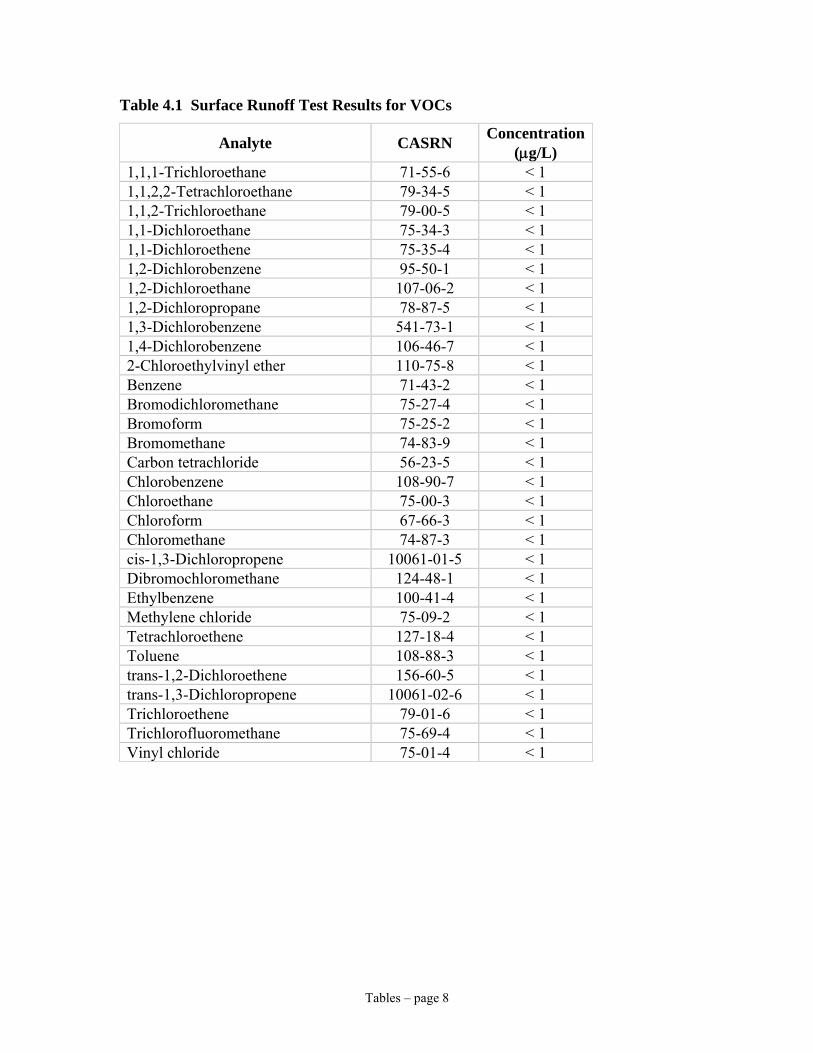
Tables – page 8
Table 4.1 Surface Runoff Test Results for VOCs
Analyte CASRN Concentration (μg/L)
1,1,1-Trichloroethane 71-55-6 < 1 1,1,2,2-Tetrachloroethane 79-34-5 < 1 1,1,2-Trichloroethane 79-00-5 < 1 1,1-Dichloroethane 75-34-3 < 1 1,1-Dichloroethene 75-35-4 < 1 1,2-Dichlorobenzene 95-50-1 < 1 1,2-Dichloroethane 107-06-2 < 1 1,2-Dichloropropane 78-87-5 < 1 1,3-Dichlorobenzene 541-73-1 < 1 1,4-Dichlorobenzene 106-46-7 < 1 2-Chloroethylvinyl ether 110-75-8 < 1 Benzene 71-43-2 < 1 Bromodichloromethane 75-27-4 < 1 Bromoform 75-25-2 < 1 Bromomethane 74-83-9 < 1 Carbon tetrachloride 56-23-5 < 1 Chlorobenzene 108-90-7 < 1 Chloroethane 75-00-3 < 1 Chloroform 67-66-3 < 1 Chloromethane 74-87-3 < 1 cis-1,3-Dichloropropene 10061-01-5 < 1 Dibromochloromethane 124-48-1 < 1 Ethylbenzene 100-41-4 < 1 Methylene chloride 75-09-2 < 1 Tetrachloroethene 127-18-4 < 1 Toluene 108-88-3 < 1 trans-1,2-Dichloroethene 156-60-5 < 1 trans-1,3-Dichloropropene 10061-02-6 < 1 Trichloroethene 79-01-6 < 1 Trichlorofluoromethane 75-69-4 < 1 Vinyl chloride 75-01-4 < 1
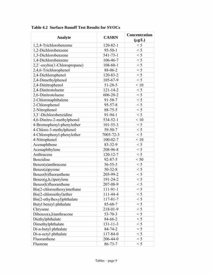
Tables – page 9
Table 4.2 Surface Runoff Test Results for SVOCs
Analyte CASRN Concentration (μg/L)
1,2,4-Trichlorobenzene 120-82-1 < 5 1,2-Dichlorobenzene 95-50-1 < 5 1,3-Dichlorobenzene 541-73-1 < 5 1,4-Dichlorobenzene 106-46-7 < 5 2,2´-oxybis(1-Chloropropane) 108-60-1 < 5 2,4,6-Trichlorophenol 88-06-2 < 5 2,4-Dichlorophenol 120-83-2 < 5 2,4-Dimethylphenol 105-67-9 < 5 2,4-Dinitrophenol 51-28-5 < 10 2,4-Dinitrotoluene 121-14-2 < 5 2,6-Dinitrotoluene 606-20-2 < 5 2-Chloronaphthalene 91-58-7 < 5 2-Chlorophenol 95-57-8 < 5 2-Nitrophenol 88-75-5 < 5 3,3´-Dichlorobenzidine 91-94-1 < 5 4,6-Dinitro-2-methylphenol 534-52-1 < 10 4-Bromophenyl-phenylether 101-55-3 < 5 4-Chloro-3-methylphenol 59-50-7 < 5 4-Chlorophenyl-phenylether 7005-72-3 < 5 4-Nitrophenol 100-02-7 < 10 Acenaphthene 83-32-9 < 5 Acenaphthylene 208-96-8 < 5 Anthracene 120-12-7 < 5 Benzidine 92-87-5 < 50 Benzo(a)anthracene 56-55-3 < 5 Benzo(a)pyrene 50-32-8 < 5 Benzo(b)fluoranthene 205-99-2 < 5 Benzo(g,h,i)perylene 191-24-2 < 5 Benzo(k)fluoranthene 207-08-9 < 5 Bis(2-chloroethoxy)methane 111-91-1 < 5 Bis(2-chloroethyl)ether 111-44-4 < 5 Bis(2-ethylhexyl)phthalate 117-81-7 < 5 Butyl benzyl phthalate 85-68-7 < 5 Chrysene 218-01-9 < 5 Dibenzo(a,h)anthracene 53-70-3 < 5 Diethylphthalate 84-66-2 < 5 Dimethylphthalate 131-11-3 < 5 Di-n-butyl phthalate 84-74-2 < 5 Di-n-octyl phthalate 117-84-0 < 5 Fluoranthene 206-44-0 < 5 Fluorene 86-73-7 < 5

Tables – page 10
Analyte CASRN Concentration (μg/L)
Hexachlorobenzene 118-74-1 < 5 Hexachlorobutadiene 87-68-3 < 5 Hexachlorocyclopentadiene 77-47-4 < 5 Hexachloroethane 67-72-1 < 5 Indeno(1,2,3-cd)pyrene 193-39-5 < 5 Isophorone 78-59-1 < 5 Naphthalene 91-20-3 < 5 Nitrobenzene 98-95-3 < 5 N-Nitrosodimethylamine 62-75-9 < 5 N-Nitroso-di-n-propylamine 621-64-7 < 5 N-Nitrosodiphenylamine 86-30-6 < 5 Pentachlorophenol 87-86-5 < 5 Phenanthrene 85-01-8 < 5 Phenol 108-95-2 < 5 Pyrene 129-00-0 < 5 2(3H)-Furanone, dihydro-4-hydroxy- a 5469-16-9 2
a Tentatively identified compound – reported based on presumptive evidence and reported as estimated concentration
Table 4.3 Surface Runoff Test Results for Metals a
Analyte CASRN Concentration (μg/L)
Surface water standard b
(μg/L) Antimony 7440-36-0 < 2.3 3 Arsenic 7440-38-2 < 1.8 50
Beryllium 7440-41-7 < 0.096 1100 Cadmium 7440-43-9 < 0.35 5 Chromium 7440-47-3 2.2 50
Copper 7440-50-8 5.4 200 Lead 7440-92-1 1.7 50
Mercury 7440-97-6 < 0.13 0.7 Nickel 7440-02-0 8.8 100
Selenium 7440-49-2 < 1.9 10 Silver 7440-22-4 < 0.54 50
Thallium 7440-28-0 < 1.9 8 Zinc 7440-66-6 59.5 82.6
a Results based on one sample collected b Assume water hardness = 100 ppm

Tables – page 11
Table 4.4 Groundwater Field Information
Turf Field #
Turf Field Area (ft2)
Depth to groundwater
(ft)
Age of Field
# Samples
# Wells
1 531,000 68.5 - 70.0 4-5 years 6 2 2 120,000 11.3 - 12.0 < 1 year 8 2 3 82,300 36.8 - 38.0 4-7 years 10 3 4 77,400 8.3 - 8.9 2-4 years 8 2
Table 4.5 Groundwater Test Results for Selected SVOCs
Analyte CASRN Concentration (μg/L) Aniline 62-53-3 < 0.39 Phenol 108-95-2 < 0.59
Benzothiazole 95-16-9 < 0.83 Table 4.6 Groundwater Test Results for all SVOCs
Analyte CASRN Concentration (μg/L) Acenaphthene 83-32-9 < 0.38
Acenaphthylene 208-96-8 < 0.72 Aniline 62-53-3 < 0.39
Anthracene 120-12-7 < 0.5 Benz(a)anthracene 56-55-3 < 0.24
Benzo(a)pyrene 50-32-8 < 0.5 Benzo(b)fluoranthene 205-99-2 < 0.36 Benzo(g,h,i)perylene 191-24-2 < 0.3 Benzo(k)fluoranthene 207-08-9 < 0.33
Benzothiazole 95-16-9 < 0.83 Benzyl Alcohol 100-51-6 < 0.55
Butyl Benzyl Phthalate 85-68-7 < 0.64 Di-n-butyl Phthalate 84-74-2 < 0.65
Carbazole 86-74-8 < 0.42 Indeno(1,2,3-cd)pyrene 193-39-5 < 0.44
4-Chloroaniline 106-47-8 < 0.63 Bis(2-chloroethoxy)methane 111-91-1 < 0.66
Bis(2-chloroethyl) Ether 111-44-4 < 0.63 2-Chloronaphthalene 91-58-7 < 0.66
2-Chlorophenol 95-57-8 < 0.32 Bis(1-chloroisopropyl) Ether 108-60-1 < 0.67
Chrysene 218-01-9 < 0.6 Dibenz(a,h)anthracene 53-70-3 < 0.32
Dibenzofuran 132-64-9 < 0.49 1,3-Dichlorobenzene 541-73-1 < 0.6 1,2-Dichlorobenzene 95-50-1 < 0.86 1,4-Dichlorobenzene 106-46-7 < 0.28

Tables – page 12
Analyte CASRN Concentration (μg/L) 3,3'-Dichlorobenzidine 91-94-1 < 0.46
2,4-Dichlorophenol 120-83-2 < 0.59 Diethyl Phthalate 84-66-2 < 0.55
Dimethyl Phthalate 131-11-3 < 0.7 2,4-Dimethylphenol 105-67-9 < 1.6 2,4-Dinitrophenol 51-28-5 < 21 2,4-Dinitrotoluene 121-14-2 < 0.68 2,6-Dinitrotoluene 606-20-2 < 0.75
Bis(2-ethylhexyl) Phthalate 117-81-7 < 0.27 Fluoranthene 206-44-0 < 0.44
Fluorene 86-73-7 < 0.55 Hexachlorobenzene 118-74-1 < 0.42
Hexachlorobutadiene 87-68-3 < 0.6 Hexachlorocyclopentadiene 77-47-4 < 0.53
Hexachloroethane 67-72-1 < 0.7 Isophorone 78-59-1 < 0.56
2-Methylnaphthalene 91-57-6 < 0.42 4,6-Dinitro-2-methylphenol 534-52-1 < 0.86 4-Chloro-3-methylphenol 59-50-7 < 0.72
2-Methylphenol 95-48-7 < 0.54 4-Methylphenol 106-44-5 < 0.78
Naphthalene 91-20-3 < 0.49 2-Nitroaniline 88-74-4 < 14 3-Nitroaniline 99-09-2 < 9.3 4-Nitroaniline 100-01-6 < 10 Nitrobenzene 98-95-3 < 0.59 2-Nitrophenol 88-75-5 < 0.76 4-Nitrophenol 100-02-7 < 6.2
N-Nitrosodimethylamine 62-75-9 < 0.43 N-Nitrosodiphenylamine 86-30-6 < 0.47
Di-n-octyl Phthalate 117-84-0 < 0.63 Pentachlorophenol (PCP) 87-86-5 < 16
Phenanthrene 85-01-8 < 0.31 Phenol 108-95-2 < 0.59
4-Bromophenyl Phenyl Ether 101-55-3 < 0.67 4-Chlorophenyl Phenyl Ether 7005-72-3 < 0.4 N-Nitrosodi-n-propylamine 621-64-7 < 0.37
Pyrene 129-00-0 < 0.44 1,2,4-Trichlorobenzene 120-82-1 < 0.62 2,4,6-Trichlorophenol 88-06-2 < 0.43 2,4,5-Trichlorophenol 95-95-4 < 0.55

Tables – page 13
Table 5.1 Predicted Groundwater Concentrations for Crumb Rubber Derived from Truck and Mixed Tires Using a Dilution Attenuation Factor (DAF) of 100 for Organics.
Facility#1 Truck Tires
Facility #4 Mixed Tires
Compound
Groundwater Quality
Standards/ Guidance Values
(μg/L)
SPLP a (μg/L)
GW Conc. (μg/L)
SPLP a (μg/L)
GW Conc. (μg/L)
Aniline 5 347 3.5 124 1.2 Phenol 1 6 0.1 23 0.2 Benzothiazole No Standard b 1,062 10.1 394 3.9 Zincc 2000 7,700 192.5 1,400 35.0 a 95% Upper Confidence Limit b Unspecified Organic Compound (UOC) standard of 50 µg/L is used for comparison purposes c NYSDEC uses a DAF of 40 for metals.
Table 6.1 Surface Water Standards for Compounds of Concern
Facility #1 Truck Tires Facility #4 Mixed Tires
Compound SPLP
Test a Column
Test a SPLP Test a
Column Test a
Surface Water Standard
(μg/L) for Stream Classes B, C, D
Zinc 7,700 436 1,400 375 117.2/82.6 b Phenol 6 1 23 2 5 Aniline 347 52 124 26 No Standard Benzothiazole 1,062 265 394 105 No Standard a 95% Upper Confidence Limit b For acute and chronic water quality standards for zinc, respectively, assuming hardness = 100 ppm. See Appendix E1 for calculations of surface water standards.

Tables – page 14
Table 7.1 Sampling Locations
Sampling Location Sampling Height Duplicate Sample Upwind edge of field 3 feet Yes On field in shade 0.4-0.8 inches & 3 feet No On field in center 0.4-0.8 inches , 3 feet, 6 feet No Downwind edge of field 0.4-0.8 inches , 3 feet, 6 feet Yes at 3 foot height
Table 7.2 Modifications to Method TO-13A
Requirement TO-13A ATL Modifications
Extraction Solvent
10% ether in hexane for PUF; methylene chloride (DCM) for XAD sorbent. Final extract in hexane.
DCM for PUF/XAD cartridge and XAD sorbent. Final extract in DCM.
Glassware Cleaning Muffle furnace is utilized. Solvent cleaning procedure is
used. Extraction technique Soxhlet extraction Soxhlet extraction or pressurized
fluid extraction (PFE). Calibration range 0.10 to 2.5 μg/mL 1.0 μg/mL to 160 μg/mL
Field surrogates Deuterated polycyclic aromatic hydrocarbons (PAHs) are spiked on media prior to sampling.
Performed by client request only.
Solvent Process Blank Required each analytical batch. Not performed; each solvent lot
is certified prior to use. Method Blank <Method Detection Limit <Reporting Limit
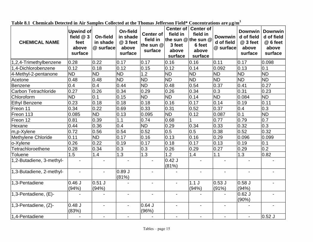
Tables – page 15
Table 8.1 Chemicals Detected in Air Samples Collected at the Thomas Jefferson Field* Concentrations are μg/m3
CHEMICAL NAME
Upwind of field @ 3
feet above
surface
On-field in shade
@ surface
On-field in shade @ 3 feet above
surface
Center of field in
the sun @ surface
Center of field in
the sun @ 3 feet above
surface
Center of field in
the sun @ 6 feet above
surface
Downwind of field
@ surface
Downwind of field @ 3 feet above
surface
Downwind of field @ 6 feet above
surface
1,2,4-Trimethylbenzene 0.28 0.22 0.17 0.17 0.16 0.16 0.11 0.17 0.098 1,4-Dichlorobenzene 0.12 0.18 0.12 0.15 0.12 0.14 0.092 0.13 0.1 4-Methyl-2-pentanone ND ND ND 1.2 ND ND ND ND ND Acetone 0.48 0.48 ND ND ND ND ND ND ND Benzene 0.4 0.4 0.44 ND 0.48 0.54 0.37 0.41 0.27 Carbon Tetrachloride 0.27 0.26 0.34 0.29 0.26 0.34 0.3 0.31 0.23 Chloroform ND 0.1 0.15 ND ND 0.14 ND 0.084 ND Ethyl Benzene 0.23 0.18 0.18 0.18 0.16 0.17 0.14 0.19 0.11 Freon 11 0.34 0.22 0.69 0.33 0.31 0.52 0.37 0.4 0.3 Freon 113 0.085 ND 0.13 0.095 ND 0.12 0.087 0.1 ND Freon 12 0.81 0.39 1.1 0.74 0.68 1 0.77 0.79 0.7 Hexane 0.44 0.36 0.4 ND 0.29 0.34 0.33 0.32 0.3 m,p-Xylene 0.72 0.56 0.54 0.52 0.5 0.5 0.38 0.52 0.32 Methylene Chloride 0.11 ND 0.17 0.16 0.13 0.16 0.29 0.096 0.099 o-Xylene 0.26 0.22 0.19 0.17 0.18 0.17 0.13 0.19 0.1 Tetrachloroethene 0.28 0.34 0.3 0.3 0.26 0.29 0.27 0.29 0.2 Toluene 1.5 1.4 1.3 1.3 1.2 1.4 1.1 1.3 0.82 1,2-Butadiene, 3-methyl- - - - - 0.42 J
(81%) - - - -
1,3-Butadiene, 2-methyl- - - 0.89 J (81%)
- - - - - -
1,3-Pentadiene 0.46 J (94%)
0.51 J (94%)
- - - 1.1 J (94%)
0.53 J (91%)
0.58 J (94%)
-
1,3-Pentadiene, (E)- - - - - - - - 0.62 J (90%)
-
1,3-Pentadiene, (Z)- 0.48 J (83%)
- - 0.64 J (96%)
- - - - -
1,4-Pentadiene - - - - - - - - 0.52 J
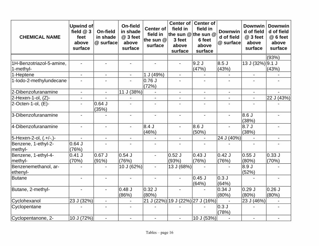
Tables – page 16
CHEMICAL NAME
Upwind of field @ 3
feet above
surface
On-field in shade
@ surface
On-field in shade @ 3 feet above
surface
Center of field in
the sun @ surface
Center of field in
the sun @ 3 feet above
surface
Center of field in
the sun @ 6 feet above
surface
Downwind of field
@ surface
Downwind of field @ 3 feet above
surface
Downwind of field @ 6 feet above
surface
(93%) 1H-Benzotriazol-5-amine, 1-methyl-
- - - - - 9.2 J (47%)
8.5 J (43%)
13 J (32%) 9.1 J (43%)
1-Heptene - - - 1 J (49%) - - - - - 1-Iodo-2-methylundecane - - - 0.76 J
(72%) - - - - -
2-Dibenzofuranamine - - 11 J (38%) - - - - - - 2-Hexen-1-ol, (Z)- - - - - - - - - 22 J (43%)2-Octen-1-ol, (E)- - 0.64 J
(35%) - - - - - - -
3-Dibenzofuranamine - - - - - - - 8.6 J (38%)
-
4-Dibenzofuranamine - - - 8.4 J (46%)
- 8.6 J (50%)
- 8.7 J (38%)
-
5-Hexen-2-ol, (.+/-.)- - - - - - - 24 J (40%) - - Benzene, 1-ethyl-2-methyl-
0.64 J (76%)
- - - - - - - -
Benzene, 1-ethyl-4-methyl-
0.41 J (70%)
0.67 J (91%)
0.54 J (76%)
- 0.52 J (93%)
0.43 J (76%)
0.42 J (76%)
0.55 J (80%)
0.33 J (70%)
Benzenemethanol, ar-ethenyl-
- - 10 J (62%) - 13 J (68%) - - 8.9 J (52%)
-
Butane - - - - - 0.45 J (64%)
0.3 J (64%)
- -
Butane, 2-methyl- - - 0.48 J (86%)
0.32 J (80%)
- - 0.34 J (80%)
0.29 J (80%)
0.26 J (80%)
Cyclohexanol 23 J (32%) - - 21 J (22%) 19 J (22%) 27 J (16%) - 23 J (46%) - Cyclopentane - - - - - - 0.3 J
(78%) - -
Cyclopentanone, 2- 10 J (72%) - - - - 10 J (53%) - - -

Tables – page 17
CHEMICAL NAME
Upwind of field @ 3
feet above
surface
On-field in shade
@ surface
On-field in shade @ 3 feet above
surface
Center of field in
the sun @ surface
Center of field in
the sun @ 3 feet above
surface
Center of field in
the sun @ 6 feet above
surface
Downwind of field
@ surface
Downwind of field @ 3 feet above
surface
Downwind of field @ 6 feet above
surface
methyl- Decanal - - - 0.46 J
(90%) - - - - -
Decane 1.2 J (53%)
- 1.2 J (64%)
1.4 J (87%)
1.2 J (64%)
1.3 J (64%)
1 J (64%) 1.3 J (64%)
0.93 J (64%)
Decane, 2,5,6-trimethyl- 0.89 J (42%)
- - - - - - - -
Decane, 2,9-dimethyl- - 1.4 J (64%)
- - - - - - -
Decane, 5-methyl- 0.28 J (50%)
- - - - - - - -
Decane, 6-ethyl-2-methyl- - - - - - - - 1.2 J (64%)
-
Dodecanal 0.38 J (72%)
- - - - - - 0.37 J (59%)
-
Heptane 0.31 J (91%)
0.43 J (86%)
- 0.36 J (74%)
- - - 0.3 J (87%)
-
Heptane, 2,3,4-trimethyl- - - 0.38 J (50%)
- - - - - -
Hexane, 3-methyl- 0.29 J (87%)
- - - - - - - -
Methanimidamide, N,N-dimethyl-N'-phenyl-
- - - - 9.6 J (72%)
- - - -
Nonanal 0.59 J (72%)
0.88 J (58%)
0.54 J (56%)
- 0.76 J (72%)
- 0.5 J (64%)
0.75 J (59%)
0.34 J (53%)
Nonanamide - - - - - 13 J (50%) - - - Nonane 1.1 J
(72%) 1.4 J (45%)
1 J (76%) 1 J (90%) 0.99 J (70%)
2.5 J (90%)
0.81 J (47%)
0.99 J (66%)
2.3 J (91%)
Octane, 2-methyl- - - - - - - - - 0.26 J

Tables – page 18
CHEMICAL NAME
Upwind of field @ 3
feet above
surface
On-field in shade
@ surface
On-field in shade @ 3 feet above
surface
Center of field in
the sun @ surface
Center of field in
the sun @ 3 feet above
surface
Center of field in
the sun @ 6 feet above
surface
Downwind of field
@ surface
Downwind of field @ 3 feet above
surface
Downwind of field @ 6 feet above
surface
(72%) Pentadecane 0.46 J
(90%) - - - - - - - -
Pentanamide, 4-methyl- - - - - 15 J (50%) - - - - Pentane, 2,2,3,4-tetramethyl-
- - - - 0.31 J (72%)
- - - -
Pentane, 2-methyl- 0.4 J (91%)
- - - - - - 0.28 J (90%)
-
Propane, 2-methyl- - - 0.4 J (4%) - - - - - - Tetradecane, 1-chloro- - - - - - 0.42 J
(74%) - - -
Undecane 0.51 J (91%)
0.58 J (90%)
0.42 J (91%)
- 0.49 J (90%)
0.45 J (81%)
0.41 J (76%)
0.49 J (91%)
0.33 J (81%)
Undecane, 2,6-dimethyl- - - - - - - - - 0.26 J (50%)
Undecane, 3-methyl- 1.1 J (53%)
- - - - - - - -
Undecane, 5,6-dimethyl- - - - - - - - 0.34 J (50%)
-
ND = not detected J = estimated concentration of a tentatively identified compound (TIC) - = not reported (%) = match quality * Chemicals that did not meet the laboratory/field blank criterion are not included.
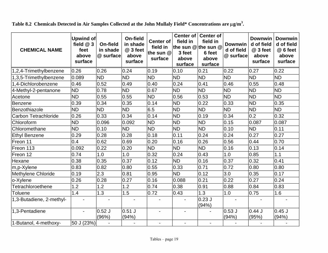
Tables – page 19
Table 8.2 Chemicals Detected in Air Samples Collected at the John Mullaly Field* Concentrations are μg/m3.
CHEMICAL NAME
Upwind of field @ 3
feet above
surface
On-field in shade
@ surface
On-field in shade @ 3 feet above
surface
Center of field in
the sun @ surface
Center of field in
the sun @ 3 feet above
surface
Center of field in
the sun @ 6 feet above
surface
Downwind of field
@ surface
Downwind of field @ 3 feet above
surface
Downwind of field @ 6 feet above
surface
1,2,4-Trimethylbenzene 0.26 0.26 0.24 0.19 0.10 0.21 0.22 0.27 0.22 1,3,5-Trimethylbenzene 0.089 ND ND ND ND ND ND ND ND 1,4-Dichlorobenzene 0.46 0.52 0.49 0.40 0.24 0.41 0.46 0.55 0.48 4-Methyl-2-pentanone ND 0.78 ND 0.67 ND ND ND ND ND Acetone ND 0.55 0.55 ND 0.56 0.53 ND ND ND Benzene 0.39 0.34 0.35 0.14 ND 0.22 0.33 ND 0.35 Benzothiazole ND ND ND 6.5 ND ND ND ND ND Carbon Tetrachloride 0.26 0.33 0.34 0.14 ND 0.19 0.34 0.2 0.32 Chloroform ND 0.096 0.092 ND ND ND 0.15 0.087 0.087 Chloromethane ND 0.10 ND ND ND ND 0.10 ND 0.11 Ethyl Benzene 0.29 0.28 0.28 0.18 0.11 0.24 0.24 0.27 0.27 Freon 11 0.4 0.62 0.69 0.20 0.16 0.26 0.56 0.44 0.70 Freon 113 0.092 0.22 0.20 ND ND ND 0.16 0.13 0.14 Freon 12 0.74 1.0 1.0 0.32 0.24 0.43 1.0 0.85 1.1 Hexane 0.38 0.35 0.37 0.12 ND 0.16 0.37 0.32 0.41 m,p-Xylene 0.83 0.82 0.80 0.55 0.33 0.71 0.72 0.80 0.80 Methylene Chloride 0.19 2.3 0.81 0.95 ND 0.12 3.0 0.35 0.17 o-Xylene 0.26 0.28 0.27 0.16 0.088 0.21 0.22 0.27 0.24 Tetrachloroethene 1.2 1.2 1.2 0.74 0.38 0.91 0.88 0.84 0.83 Toluene 1.4 1.3 1.5 0.72 0.43 1.3 1.0 0.75 1.6 1,3-Butadiene, 2-methyl- - - - - - 0.23 J
(94%) - - -
1,3-Pentadiene - 0.52 J (96%)
0.51 J (94%)
- - - 0.53 J (94%)
0.44 J (95%)
0.45 J (94%)
1-Butanol, 4-methoxy- 50 J (23%) - - - - - - - -

Tables – page 20
CHEMICAL NAME
Upwind of field @ 3
feet above
surface
On-field in shade
@ surface
On-field in shade @ 3 feet above
surface
Center of field in
the sun @ surface
Center of field in
the sun @ 3 feet above
surface
Center of field in
the sun @ 6 feet above
surface
Downwind of field
@ surface
Downwind of field @ 3 feet above
surface
Downwind of field @ 6 feet above
surface
1-Hexene, 3,4,5-trimethyl- 1.5 J (59%)
0.45 J (59%)
- - - - - - -
1-Hexene, 4,5-dimethyl- - - - - - - 0.33 J (64%)
- -
1-Propene, 2-methyl- - - - 0.46 J (80%)
0.33 J (80%)
1.0 J (50%)
- - -
2-Butene, (E)- - 1.8 J (52%)
- - - 0.54 J (80%)
- 0.56 J (59%)
-
2-Butene, (Z)- 2.8 J (50%)
- 2.7 J (50%)
0.55 J (64%)
0.23 J (59%)
- 0.88 J (42%)
- 1.1 J (53%)
2-Dibenzofuranamine - - - - - - - 12 J (38%) - 3-Dibenzofuranamine - 10 J
(38%) - - - - 11 J
(38%) 9.9 J (38%)
-
3H-Indazol-3-one, 1,2-dihydro-2-methyl-
14 J (53%) - - - - - - - 12 J (53%)
4-Dibenzofuranamine 9.0 J (46%)
- - 10 J (44%) 8.9 J (43%)
9.1 J (35%)
- - 11 J (43%)
Benzaldehyde, ethyl- - 9.6 J (91%)
- - - - - - -
Benzene, 1,3-dimethyl- 9.2 J (53%)
- - - - - - - -
Benzene, 1-ethyl-2-methyl-
1.8 J (80%)
- - - - - - 0.59 J (86%)
0.51 J (55%)
Benzene, 1-ethyl-3-methyl-
- - 0.51 J (55%)
- - - - - -
Benzene, 1-ethyl-4-methyl-
0.48 J (60%)
0.56 J (87%)
- - - - 0.49 J (86%)
- -
Benzene, 1-methoxy-4-(1-propenyl)-
- - - - 9.9 J (52%)
- 9.7 J (45%)
- -

Tables – page 21
CHEMICAL NAME
Upwind of field @ 3
feet above
surface
On-field in shade
@ surface
On-field in shade @ 3 feet above
surface
Center of field in
the sun @ surface
Center of field in
the sun @ 3 feet above
surface
Center of field in
the sun @ 6 feet above
surface
Downwind of field
@ surface
Downwind of field @ 3 feet above
surface
Downwind of field @ 6 feet above
surface
Benzene, 2-methoxy-1,3,4-trimethyl-
- - - 2.1 J (17%)
- - - - -
Benzo[b]thiophene, 6-methyl-
- - - - - 8.7 J (53%)
- - -
Butane - 0.50 J (38%)
0.43 J (38%)
- - - 0.42 J (52%)
0.33 J (56%)
0.41 J (64%)
Butane, 2-iodo-2-methyl- 0.34 J (72%)
- - - - 0.35 J (64%)
- - -
Butane, 2-methyl- 0.42 J (80%)
0.65 J (80%)
0.61 J (80%)
0.22 J (80%)
- - 0.50 J (80%)
0.31 J (80%)
0.42 J (80%)
Cycloheptane - - - - - - - 0.23 J (27%)
-
Cyclohexane, 1,1,3-trimethyl-
- - 0.60 J (86%)
- - - - - -
Cyclohexane, 1,3-dimethyl-, cis
0.94 J (94%)
- - - - 0.47 J (95%)
0.44 J (95%)
0.42 J (94%)
0.48 J (94%)
Cyclohexane, 1,4-dimethyl-
- - 1.1 J (91%)
- - - - - -
Cyclohexane, ethyl- 1 J (87%) 1.3 J (64%)
- 0.38 J (87%)
- 0.55 J (90%)
0.47 J (68%)
0.52 J (86%)
0.59 J (90%)
Cyclopropane, 1-chloro-2-ethenyl-1-methy
- - 17 J (59%) - - - 23 J (64%) 18 J (59%) -
Decane 3.3 J (53%)
1.1 J (64%)
- - 0.64 J (64%)
- 1.1 J (59%)
1.2 J (64%)
1.1 J (64%)
Decane, 2,3,8-trimethyl- 1.5 J (53%)
- - - - - - - -
Decane, 2,9-dimethyl- - - - 0.92 J (59%)
- - - - -
Dodecane, 2,6,11- 0.66 J - - 0.23 J - - - - -
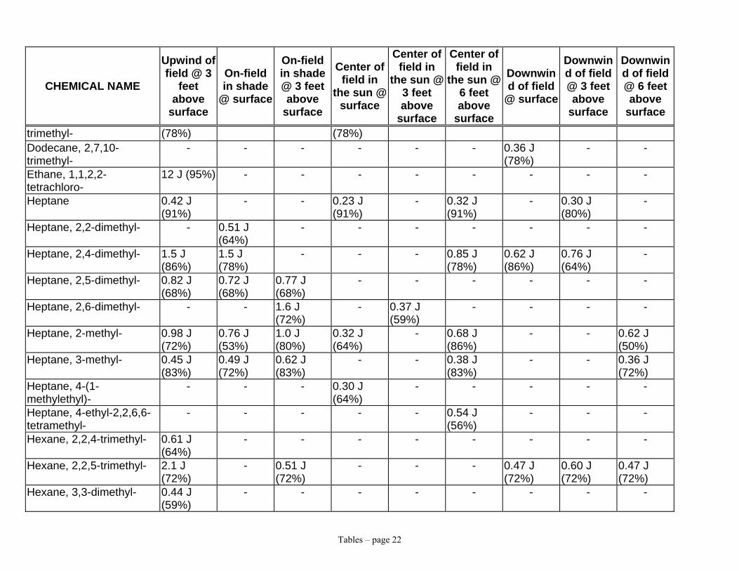
Tables – page 22
CHEMICAL NAME
Upwind of field @ 3
feet above
surface
On-field in shade
@ surface
On-field in shade @ 3 feet above
surface
Center of field in
the sun @ surface
Center of field in
the sun @ 3 feet above
surface
Center of field in
the sun @ 6 feet above
surface
Downwind of field
@ surface
Downwind of field @ 3 feet above
surface
Downwind of field @ 6 feet above
surface
trimethyl- (78%) (78%) Dodecane, 2,7,10-trimethyl-
- - - - - - 0.36 J (78%)
- -
Ethane, 1,1,2,2-tetrachloro-
12 J (95%) - - - - - - - -
Heptane 0.42 J (91%)
- - 0.23 J (91%)
- 0.32 J (91%)
- 0.30 J (80%)
-
Heptane, 2,2-dimethyl- - 0.51 J (64%)
- - - - - - -
Heptane, 2,4-dimethyl- 1.5 J (86%)
1.5 J (78%)
- - - 0.85 J (78%)
0.62 J (86%)
0.76 J (64%)
-
Heptane, 2,5-dimethyl- 0.82 J (68%)
0.72 J (68%)
0.77 J (68%)
- - - - - -
Heptane, 2,6-dimethyl- - - 1.6 J (72%)
- 0.37 J (59%)
- - - -
Heptane, 2-methyl- 0.98 J (72%)
0.76 J (53%)
1.0 J (80%)
0.32 J (64%)
- 0.68 J (86%)
- - 0.62 J (50%)
Heptane, 3-methyl- 0.45 J (83%)
0.49 J (72%)
0.62 J (83%)
- - 0.38 J (83%)
- - 0.36 J (72%)
Heptane, 4-(1-methylethyl)-
- - - 0.30 J (64%)
- - - - -
Heptane, 4-ethyl-2,2,6,6-tetramethyl-
- - - - - 0.54 J (56%)
- - -
Hexane, 2,2,4-trimethyl- 0.61 J (64%)
- - - - - - - -
Hexane, 2,2,5-trimethyl- 2.1 J (72%)
- 0.51 J (72%)
- - - 0.47 J (72%)
0.60 J (72%)
0.47 J (72%)
Hexane, 3,3-dimethyl- 0.44 J (59%)
- - - - - - - -

Tables – page 23
CHEMICAL NAME
Upwind of field @ 3
feet above
surface
On-field in shade
@ surface
On-field in shade @ 3 feet above
surface
Center of field in
the sun @ surface
Center of field in
the sun @ 3 feet above
surface
Center of field in
the sun @ 6 feet above
surface
Downwind of field
@ surface
Downwind of field @ 3 feet above
surface
Downwind of field @ 6 feet above
surface
Hydroxylamine, O-decyl- - - - - - - - - 0.88 J (64%)
Methanimidamide, N,N-dimethyl-N'-phenyl-
16 J (50%) - - 8.7 J (50%)
- - - - -
Nonanal 1.28 J (68%)
- 0.54 J (72%)
0.47 J (50%)
0.45 J (72%)
0.51 J (78%)
- - 0.42 J (53%)
Nonane 3.2 J (91%)
2.6 J (91%)
3.2 J (91%)
2.1 J (87%)
1.7 J (87%)
2.8 J (94%)
1.8 J (91%)
2.3 J (91%)
2.7 J (83%)
Nonane, 3-methyl-5-propyl-
- - - - - - - 0.33 J (72%)
-
Octane 6.3 J (90%)
4.5 J (45%)
6.2 J (46%)
3.4 J (74%)
3.0 J (49%)
5.9 J (94%)
3.1 J (70%)
4.7 J (38%)
6.0 J (76%)
Octane, 2-methyl- - - 0.41 J (72%)
- - - - - -
Octane, 3-methyl- 0.64 J (64%)
- - - - 0.42 J (90%)
- 0.39 J (80%)
0.44 J (91%)
Pentane - 0.46 J (86%)
0.40 J (86%)
- - - - - -
Pentane, 2,2,3,4-tetramethyl-
- - - 0.42 J (53%)
0.30 J (53%)
- - - -
Pentane, 2-methyl- - - - - - - 0.35 J (80%)
0.31 J (91%)
0.32 J (91%)
Pentane, 3,3-dimethyl- - - - - - 0.40 J (50%)
- 0.44 J (64%)
-
Propane, 2-methyl- - - - - - - - 0.25 J (45%)
-
Tetradecane, 1-chloro- - - - 0.56 J (74%)
- - - - -
Tridecane 0.96 J - - - - 0.96 J - - -
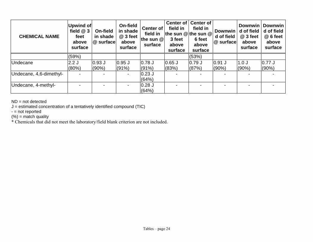
Tables – page 24
CHEMICAL NAME
Upwind of field @ 3
feet above
surface
On-field in shade
@ surface
On-field in shade @ 3 feet above
surface
Center of field in
the sun @ surface
Center of field in
the sun @ 3 feet above
surface
Center of field in
the sun @ 6 feet above
surface
Downwind of field
@ surface
Downwind of field @ 3 feet above
surface
Downwind of field @ 6 feet above
surface
(59%) (53%) Undecane 2.2 J
(80%) 0.93 J (90%)
0.95 J (91%)
0.78 J (91%)
0.65 J (83%)
0.79 J (87%)
0.91 J (90%)
1.0 J (90%)
0.77 J (90%)
Undecane, 4,6-dimethyl- - - - 0.23 J (64%)
- - - - -
Undecane, 4-methyl- - - - 0.28 J (64%)
- - - - -
ND = not detected J = estimated concentration of a tentatively identified compound (TIC) - = not reported (%) = match quality * Chemicals that did not meet the laboratory/field blank criterion are not included.

Tables – page 25
Table 8.3 TICs Detected in Laboratory and/or Field Blank Samples. Concentrations are μg/m3
Laboratory Blank Concentration
Field Blank Concentration Tentatively Identified Compound Thomas Jefferson
Field John Mullaly
Field Thomas Jefferson
Field John Mullaly
Field 2-Cyclohexen-1-ol 32J 34J 38J 40J 2-Cyclohexen-1-one 33J 35J 35J 42J 7-Oxabicyclo[4.1.0]heptane 35J 25J 32J 30J Benzene, 1-methoxy-4-(1-propenyl)- NR 12J NR NR Benzene, 2,4-diisocyanato-1-methyl- 13J 15J 9.1J 10J Bi-2-cyclohexen-1-yl 24J NR 18J NR Cyclohexanol 18J 15J NR 18J Cyclohexanol, 2-chloro-, trans- 21J 30J 20J 33J Cyclopentene, 1,5-dimethyl- NR 12J NR 15J Cyclohexanone NR NR 9.2J NR Benzene, 1,2-dimethyl- NR NR NR 10J Cyclopentanol, 2-methyl- NR NR 19J NR Tetradecane NR NR NR 0.63J Undecane, 2,3-dimethyl- NR NR 0.29J NR NR = not reported J = estimated concentration

Tables – page 26
Table 8.4 Thomas Jefferson Field – Measured Air Concentrations (μg/m3) for Chemicals Selected for Health Risk Evaluation
Air Concentration (μg/m3)*
Name
Upwind of field @ 3 ft
above surface
On-field in shade @ surface
On-field in shade @ 3 ft
above surface
Center of field in the
sun @ surface
Center of field in the sun @ 3 ft
above surface
Center of field in the sun @ 6 ft
above surface
Downwind of field @ surface
Downwind of field @ 3 ft
above surface
Downwind of field @ 6 ft
above surface
Chemicals Detected in Field Survey Also Detected in DEC Laboratory Off-gassing Study 1,4-Dichlorobenzene 0.12 0.18 0.12 0.15 0.12 0.14 0.092 0.13 0.1 4-Methyl-2-pentanone ND ND ND 1.2 ND ND ND ND ND
Benzene 0.4 0.4 0.44 ND 0.48 0.54 0.37 0.41 0.27 Benzene, 1-ethyl-4-methyl- 0.41 J (70%) 0.67 J (91%)0.54 J (76%) - 0.52 J (93%) 0.43 J (76%)0.42 J (76%)0.55 J (81%) 0.33 J (70%)
Nonane 1.1 J (72%) 1.4 J (45%) 1 J (76%) 1 J (90%) 0.99 J (70%) 2.5 J (90%) 0.81 J (47%)0.99 J (66%) 2.3 J (91%) Chemicals on Target List Detected in Field Survey Not Included in DEC Off-gassing Study
Freon 11 0.34 0.22 0.69 0.33 0.31 0.52 0.37 0.4 0.3
Freon 113 0.085 ND 0.13 0.095 ND 0.12 0.087 0.1 ND
Methylene Chloride 0.11 ND 0.17 0.16 0.13 0.16 0.29 0.096 0.099 Chemicals Detected in Field Survey Reported as Non-Detects in DEC Laboratory Off-gassing Study
Chloroform ND 0.1 0.15 ND ND 0.14 ND 0.084 ND Chemicals Detected in Field Survey as TICs
1,3-Pentadiene 0.46 J (94%) 0.51 J (94%) - - - 1.1 J (94%) 0.53 J (91%)0.58 J (94%) -
1,3-Pentadiene, (E)- - - - - - - - 0.62 J (90%) -
1,4-Pentadiene - - - - - - - - 0.52 J (93%)
Butane, 2-methyl- - - 0.48 J (86%)0.32 J (80%) - - 0.34 J (80%)0.29 J (80%) 0.26 J (80%)
Decanal - - - 0.46 J (90%) - - - - -
Heptane 0.31 J (91%) 0.43 J (86%) - 0.36 J (74%) - - - 0.3 J (87%) -

Tables – page 27
*ND = not detected; - = not reported; J = estimated concentration; (percentage) = degree of statistical match between the mass spectrum of a suspect chemical and the mass spectrum of a known chemical from a computer-based “library” of mass spectra. The suspect chemical is tentatively identified as the chemical with the highest match quality. A match of 85% or higher is necessary for reliable identification (US EPA, 1999b).
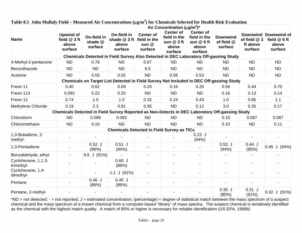
Tables – page 28
Table 8.5 John Mullaly Field – Measured Air Concentrations (μg/m3) for Chemicals Selected for Health Risk Evaluation Air Concentration (μg/m3)*
Name Upwind of field @ 3 ft
above surface
On-field in shade @ surface
On-field in shade @ 3 ft
above surface
Center of field in the
sun @ surface
Center of field in the sun @ 3 ft
above surface
Center of field in the sun @ 6 ft
above surface
Downwind of field @ surface
Downwind of field @ 3
ft above surface
Downwind of field @ 6 ft
above surface
Chemicals Detected in Field Survey Also Detected in DEC Laboratory Off-gassing Study 4-Methyl-2-pentanone ND 0.78 ND 0.67 ND ND ND ND ND Benzothiazole ND ND ND 6.5 ND ND ND ND ND Acetone ND 0.55 0.55 ND 0.56 0.53 ND ND ND
Chemicals on Target List Detected in Field Survey Not Included in DEC Off-gassing Study Freon 11 0.40 0.62 0.69 0.20 0.16 0.26 0.56 0.44 0.70 Freon 113 0.092 0.22 0.20 ND ND ND 0.16 0.13 0.14 Freon 12 0.74 1.0 1.0 0.32 0.24 0.43 1.0 0.85 1.1 Methylene Chloride 0.19 2.3 0.81 0.95 ND 0.12 3.0 0.35 0.17
Chemicals Detected in Field Survey Reported as Non-Detects in DEC Laboratory Off-gassing Study Chloroform ND 0.096 0.092 ND ND ND 0.15 0.087 0.087 Chloromethane ND 0.10 ND ND ND ND 0.10 ND 0.11
Chemicals Detected in Field Survey as TICs 1,3-Butadiene, 2-methyl- - - - - - 0.23 J
(94%) - - -
1,3-Pentadiene - 0.52 J (96%)
0.51 J (94%) -- - - 0.53 J
(94%) 0.44 J (95%) 0.45 J (94%)
Benzaldehyde, ethyl- - 9.6 J (91%) - - - - - - - Cyclohexane, 1,1,3-trimethyl- - - 0.60 J
(86%) - - - - - -
Cyclohexane, 1,4-dimethyl- - - 1.1 J (91%) - - - - - -
Pentane - 0.46 J (86%)
0.40 J (86%) - - - - - -
Pentane, 2-methyl- - - - - - - 0.35 J (80%)
0.31 J (91%) 0.32 J (91%)
*ND = not detected; - = not reported; J = estimated concentration; (percentage) = degree of statistical match between the mass spectrum of a suspect chemical and the mass spectrum of a known chemical from a computer-based “library” of mass spectra. The suspect chemical is tentatively identified as the chemical with the highest match quality. A match of 85% or higher is necessary for reliable identification (US EPA, 1999b)

Tables – page 29
Table 8.6 Toxicity Values for Chemicals Selected for Health Risk Evaluation.
Name (CASRN) Basis for Toxicity Value
Surrogate Chemical (CASRN)
Rational Reference
Concentration μg/m3 (Effect)
Air Concentration (μg/m3) at 1 x 10⁻⁶ Risk
Level
Source of Toxicity Values
Chemicals Detected in Field Survey Also Detected in DEC Laboratory Off-gassing Study 1,4-Dichlorobenzene
(106-46-7) chemical-specific NA NA* 800 (increased liver
weights in rats) 0.32 NYS (2006)
Acetone (67-64-1) chemical-specific NA NA* 30,000 (neurological
effects in humans) none
available** NYS (2006)
Benzene (71-43-2) chemical-specific NA* NA*
30 (decreased lymphocyte count in
humans) 0.13 NYS (2006)
Benzene, 1-ethyl-4-methyl- (622-96-8)
surrogate-chemical
dimethyl benzenes (xylenes)
(1330-20-7)
all are alkyl benzenes with substitutions at two positions of the
benzene ring & differ only in the structure of one of the alkyl groups attached to benzene ring; xylenes
have a peer-reviewed RfC
100 (impaired motor coordination in rats)
none available** NYS (2006)
Benzothiazole (95-16-9) chemical-specific NA* NA* 18*** (none reported) none
available** ***
4-Methyl-2-pentanone (108-10-1)
chemical specific NA* NA*
3000 (reduced fetal body wt, skeletal variations, & increased fetal death in mice; skeletal variations
in rats
none available**
US EPA IRIS#
Nonane (111-84-2) surrogate-chemical
hexane (110-54-3)
both are straight-chain alkanes; hexane among most potent alkanes &
has a peer-reviewed RfC
700 (peripheral neuropathy in rats)
none available**
US EPA IRIS#
Chemicals on Target List Detected in Field Survey Not Included in DEC Off-gassing Study Freon 11 or
trichloromonofluoromethane (75-69-4) Freon 12 or
dichlorodifluoromethane (1275-71-8)
surrogate chemical
chlorodifluoro-methane
(HCFC 22) (75-45-6)
all are halogenated methanes that differ only in the number of chlorines or fluorines attached to carbon atom; HCFC 22 has a peer-reviewed RfC
50,000 (increased kidney, adrenal & pituitary
weights in rats)
none available**
US EPA IRIS#

Tables – page 30
Name (CASRN) Basis for Toxicity Value
Surrogate Chemical (CASRN)
Rational Reference
Concentration μg/m3 (Effect)
Air Concentration (μg/m3) at 1 x 10⁻⁶ Risk
Level
Source of Toxicity Values
Freon 113 or CFC-113 or 1,1,2-trichloro-1,2,2-
trifluoroethane (76-13-1)
chemical-specific NA* NA* 190,000 (psychomotor
impairment in humans) none
available** US EPA IRIS#
Methylene Chloride (75-09-2)
chemical-specific NA* NA*
400 (blood carboxyhemoglobin
above 2% in humans) 27 NYS (2006)
Chemicals Detected in Field Survey Reported as Non-Detects in DEC Laboratory Off-gassing Study Chloroform (67-66-3) chemical-
specific NA* NA* 50 (liver & kidney toxicity in mice) 14.8 NYS (2006)
Chloromethane (74-87-3) chemical-specific NA* NA* 90 (cerebellar lesions in
mice) none
available** US EPA IRIS#
Chemicals Detected in Field Survey as TICs
Benzaldehyde, ethyl- (53951-50-1)
surrogate-chemical
benzaldehyde (100-52-7)
both are aldehydes with a benzene ring & differ only in the ethyl group of the TIC; benzaldehyde has a peer-
reviewed RfD
350**** (forestomach lesions, kidney toxicity in
rats)
none available**
US EPA IRIS#
1,3-Butadiene, 2-methyl- (78-79-5)
surrogate-chemical
1,3-butadiene (106-99-0)
both are conjugated dienes & differ only in the methyl groups of the TIC;
1,3-butadiene is a highly potent chemical and has peer-reviewed
toxicity values
2 (ovarian atrophy in mice) 0.03 US EPA
IRIS#
Butane, 2-methyl (92046-46-3)
surrogate-chemical
hexane (110-54-3)
both are straight-chain alkanes & differ only in the methyl group
attached to the carbon chain; hexaneamong most potent alkanes & has a
peer-reviewed RfC
700 (peripheral neuropathy in rats)
none available**
US EPA IRIS#
Cyclohexane, 1,4-dimethyl- (589-90-2)
Cyclohexane, 1,1,3-trimethyl- (3073-66-3)
surrogate-chemical
cyclohexane (110-82-7)
all are cycloalkanes & differ only in the methyl groups attached to the
cyclohexane ring of the TICs; cyclohexane has a peer-reviewed RfC
6000 (reduced pup weights in F1 and F2 generations in rats)
none available**
US EPA IRIS#

Tables – page 31
Name (CASRN) Basis for Toxicity Value
Surrogate Chemical (CASRN)
Rational Reference
Concentration μg/m3 (Effect)
Air Concentration (μg/m3) at 1 x 10⁻⁶ Risk
Level
Source of Toxicity Values
Decanal (112-31-2) surrogate-chemical
propanal (propionaldehyde
) (123-38-6)
both are aldehydes & differ only in the number of carbon atoms; propanal
has peer-reviewed RfC
8 (atrophy of olfactory epithelium in rats)
none available**
US EPA IRIS#
Heptane (142-82-5)
Pentane (109-66-0) surrogate-chemical
hexane (110-54-3)
all are straight-chain alkanes; hexane among most potent alkanes & has a
peer-reviewed RfC
700 (peripheral neuropathy in rats)
none available**
US EPA IRIS#
1,3-Pentadiene (504-60-9)
1,3-Pentadiene, (E)- (2004-70-8)
1,4-Pentadiene (591-93-5)
surrogate-chemical
1,3-butadiene (106-99-0)
all are conjugated dienes & differ in the number of carbon atoms; 1,3-
butadiene is a highly potent chemical & has peer-reviewed toxicity values
2 (ovarian atrophy in mice) 0.03 US EPA
IRIS#
* NA = not applicable. ** Chemicals may lack an estimate of the air concentration associated with a lifetime excess risk of one per million (1 x 10⁻⁶), assuming continuous exposure, for several different reasons: because their potency to cause cancer has not been studied, because studies of their carcinogenic potency did not show a concentration-related increase in cancer incidence or because some evidence of carcinogenic potency has been observed, but the quality of the studies or the data do not allow quantitative estimation of the 1 x 10⁻⁶ air concentration. *** Reference Concentration = [Reference dose (RfD) x Adult Body Weight]/Adult Inhalation Rate: RfC = [5 μg/kg-day x 70 kg]/20 m3/day = 18 μg /m3, where the draft reference dose is derived from a no-observed-effect level of 5 μg /kg-day in a 90-day study with rats (WHO, 2003) and the application of a 1000-fold uncertainty factor to compensate for interspecies difference, human variation, and the use of a subchronic study to estimate a chronic reference dose. **** Reference Concentration = [Reference dose (RfD) x Adult Body Weight]/Adult Inhalation Rate: RfC = [100 μg /kg-day x 70 kg]/20 m3/day = 350 μg/m3. #http://cfpub.epa.gov/ncea/iris/index.cfm References for Table 6 NYS (New York State). 2006. New York State Brownfield Cleanup Program, Development of Soil Cleanup Objectives. Technical Support Document. Albany, NY: New York State Department of Environmental Conservation and New York State Department of Health.

Tables – page 32
WHO (World Health Organization). 2003. Safety Evaluation of Certain Food Additives / prepared by the Fifty-Ninth Meeting of the Joint FAO/WHO Expert Committee on Food Additives (JECFA). WHO Food Additives Series: 50. Geneva, SZ: International Programme on Chemical Safety. [Last accessed on 12 01 08 on-line at http://www.inchem.org/documents/jecfa/jecmono/v50je01.htm]

Tables – page 33
Table 8.7 Thomas Jefferson Field – Ratio of Measured Concentration/Reference Concentration (Hazard Quotient) for Chemicals Selected for Health Risk Evaluation (see Table 8.4 for Measured Air Concentrations)
Hazard Quotient (rounded to one significant figure)*
Name Type of Toxicity Value
Upwind of field @ 3 ft
above surface
On-field in shade @ surface
On-field in shade @ 3
ft above surface
Center of field in the
sun @ surface
Center of field in the sun @ 3 ft
above surface
Center of field in the sun @ 6 ft
above surface
Downwind of field @ surface
Downwind of field @ 3
ft above surface
Downwind of field @ 6
ft above surface
Chemicals Detected in Field Survey Also Detected in DEC Laboratory Off-gassing Study 1,4-Dichlorobenzene chemical-specific 0.0002 0.0002 0.0002 0.0002 0.0002 0.0002 0.0001 0.0002 0.0001
4-Methyl-2-pentanone chemical-specific ND ND ND 0.0004 ND ND ND ND ND
Benzene chemical-specific 0.01 0.01 0.02 ND 0.02 0.02 0.01 0.01 0.009
Benzene, 1-ethyl-4-methyl-
surrogate-chemical:
xylenes (dimethyl benzenes)
0.004** 0.007** 0.005** - 0.005** 0.004** 0.004** 0.006** 0.003**
Nonane surrogate-chemical: hexane 0.002** 0.002** 0.001** 0.001** 0.001** 0.004** 0.001** 0.001** 0.003**
Chemicals on Target List Detected in Field Survey Not Included in DEC Off-gassing Study
Freon 11 surrogate-
chemical: HCFC 22
< 0.0001 < 0.0001 < 0.0001 < 0.0001 < 0.0001 < 0.0001 < 0.0001 < 0.0001 < 0.0001
Freon 113 chemical-specific < 0.0001 ND < 0.0001 < 0.0001 ND < 0.0001 < 0.0001 < 0.0001 ND
Methylene Chloride chemical-specific 0.0003 ND 0.0004 0.0004 0.0003 0.0004 0.0007 0.0002 0.0002 Chemicals Detected in Field Survey Reported as Non-Detects in DEC Laboratory Off-gassing Study
Chloroform chemical-specific ND 0.002 0.003 ND ND 0.003 ND 0.002 ND Chemicals Detected in Field Survey as TICs
1,3-Pentadiene surrogate-
chemical: 1,3-butadiene
0.2** 0.3** - - - 0.6** 0.3** 0.3** -
1,3-Pentadiene, (E)- surrogate-
chemical: 1,3-butadiene
- - - - - - - 0.3** -

Tables – page 34
Hazard Quotient (rounded to one significant figure)*
Name Type of Toxicity Value
Upwind of field @ 3 ft
above surface
On-field in shade @ surface
On-field in shade @ 3
ft above surface
Center of field in the
sun @ surface
Center of field in the sun @ 3 ft
above surface
Center of field in the sun @ 6 ft
above surface
Downwind of field @ surface
Downwind of field @ 3
ft above surface
Downwind of field @ 6
ft above surface
1,4-Pentadiene surrogate-
chemical: 1,3-butadiene
- - - - - - - - 0.3**
Butane, 2-methyl- surrogate-chemical: hexane _ - 0.0007** 0.0005** - - 0.0005** 0.0004*** 0.0004**
Decanal
surrogate-chemical: propanal
(propionaldehyde)
- - - 0.06** - - - - -
Heptane surrogate-chemical: hexane 0.0004** 0.0006** - 0.0005** - - - 0.0004** -
*ND = not detected; - = not reported. ** Based on estimated chemical concentration and tentative chemical identification.

Tables – page 35
Table 8.8 Thomas Jefferson Field – Estimated Excess Cancer Risks from Continuous Lifetime Exposure at Measured Air Concentrations of Known or Potential Cancer-Causing Chemicals Selected for Health Risk Evaluation (see Table 8.4 for Measured Air Concentrations)
Excess Lifetime Risk (rounded to one significant figure)*
Name Type of Toxicity Value
Upwind of field @ 3 ft
above surface
On-field in shade @ surface
On-field in shade @ 3
ft above surface
Center of field in the
sun @ surface
Center of field in the sun @ 3 ft
above surface
Center of field in the sun @ 6 ft
above surface
Downwind of field @ surface
Downwind of field @ 3
ft above surface
Downwind of field @ 6
ft above surface
Chemicals Detected in Field Survey Also Detected in DEC Laboratory Off-gassing Study 1,4-Dichlorobenzene chemical-specific 0.4 x 10⁻⁶ 0.6 x 10⁻⁶ 0.4 x 10⁻⁶ 0.5 x 10⁻⁶ 0.4 x 10⁻⁶ 0.4 x 10⁻⁶ 0.3 x 10⁻⁶ 0.4 x 10⁻⁶ 0.3 x 10⁻⁶
Benzene chemical-specific 3 x 10⁻⁶ 3 x 10⁻⁶ 3 x 10⁻⁶ ND 4 x 10⁻⁶ 4 x 10⁻⁶ 3 x 10⁻⁶ 3 x 10⁻⁶ 2 x 10⁻⁶
Chemicals on Target List Detected in Field Survey Not Included in DEC Off-gassing Study Methylene Chloride chemical-specific 0.004 x 10⁻⁶ ND 0.006 x 10⁻⁶ 0.006 x 10⁻⁶ 0.005 x 10⁻⁶ 0.006 x 10⁻⁶ 0.01 x 10⁻⁶ 0.004 x 10⁻⁶ 0.004 x 10⁻⁶
Chemicals Detected in Field Survey Reported as Non-Detects in DEC Laboratory Off-gassing Study Chloroform chemical-specific ND 0.007 x 10⁻⁶ 0.01 x 10⁻⁶ ND ND 0.009 x 10⁻⁶ ND 0.006 x 10⁻⁶ ND
Chemicals Detected in Field Study as TICs
1,3-Pentadiene surrogate-
chemical: 1,3-butadiene
2 x 10⁻⁵** 2 x 10⁻⁵** - - - 4 x 10⁻⁵** 2 x 10⁻⁵** 2 x 10⁻⁵** -
1,3-Pentadiene, (E)- surrogate-
chemical: 1,3-butadiene
- - - - - - - 2 x 10⁻⁵** -
1,4-Pentadiene surrogate-
chemical 1,3-butadiene
- - - - - - - - 2 x 10⁻⁵**
** ND = not detected; - = not reported. ** Based on estimated chemical concentration and tentative chemical identification.

Tables - page 36
Table 8.9 John Mullaly Field – Ratio of Measured Concentration/Reference Concentration (Hazard Quotient) for Chemicals Selected for Health Risk Evaluation (see Table 5 for Measured Air Concentrations)
Hazard Quotient (rounded to one significant figure)*
Name Type of Toxicity Value
Upwind of field @ 3 ft
above surface
On-field in shade @ surface
On-field in shade @ 3 ft
above surface
Center of field in the
sun @ surface
Center of field in the sun @ 3 ft
above surface
Center of field in the sun @ 6 ft
above surface
Downwind of field @ surface
Downwind of field @ 3
ft above surface
Downwind of field @ 6
ft above surface
Chemicals Detected in Field Survey Also Detected in DEC Laboratory Off-gassing Study 4-Methyl-2-pentanone chemical-specific ND 0.0003 ND 0.0002 ND ND ND ND ND
Acetone chemical-specific ND 0.00002 0.00002 ND 0.00002 0.00002 ND ND ND Benzothiazole default value ND ND ND 0.4 ND ND ND ND ND
Chemicals on Target List Detected in Field Survey Not Included in DEC Off-gassing Study
Freon 11 surrogate-
chemical: HCFC 22
< 0.00001 0.00001 0.00001 < 0.00001 < 0.00001 < 0.00001 0.00001 < 0.00001 0.00001
Freon 113 chemical-specific < 0.00001 < 0.00001 < 0.00001 ND ND ND < 0.00001 < 0.00001 < 0.00001
Freon 12 surrogate-
chemical: HCFC 22
0.00001 0.00002 0.00002 < 0.00001 < 0.00001 < 0.00001 0.00002 0.00002 0.00002
Methylene Chloride chemical-specific 0.0005 0.006 0.002 0.002 ND 0.0003 0.008 0.0009 0.0004
Chemicals Detected in Field Survey Reported as Non-Detects in DEC Laboratory Off-gassing Study Chloroform chemical-specific ND 0.002 0.002 ND ND ND 0.003 0.002 0.002 Chloromethane chemical-specific ND 0.001 ND ND ND ND 0.001 ND 0.001
Chemicals Detected in Field Survey as TICs 1,3-Butadiene, 2-methyl-
surrogate-chemical: 1,3-
butadiene - - - - - 0.1** - - -
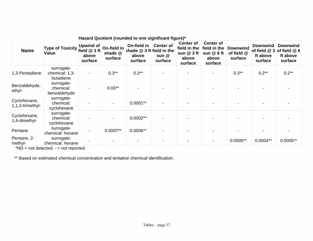
Tables – page 37
Hazard Quotient (rounded to one significant figure)*
Name Type of Toxicity Value
Upwind of field @ 3 ft
above surface
On-field in shade @ surface
On-field in shade @ 3 ft
above surface
Center of field in the
sun @ surface
Center of field in the sun @ 3 ft
above surface
Center of field in the sun @ 6 ft
above surface
Downwind of field @ surface
Downwind of field @ 3
ft above surface
Downwind of field @ 6
ft above surface
1,3-Pentadiene surrogate-
chemical: 1,3-butadiene
- 0.3** 0.3** - - - 0.3** 0.2** 0.2**
Benzaldehyde, ethyl-
surrogate-chemical:
benzaldehyde - 0.03** - - - - - - -
Cyclohexane, 1,1,3-trimethyl-
surrogate-chemical:
cyclohexane - - 0.0001** - - - - - -
Cyclohexane, 1,4-dimethyl-
surrogate-chemical:
cyclohexane - - 0.0002** - - - - - -
Pentane surrogate-chemical: hexane - 0.0007** 0.0006** - - - - - -
Pentane, 2-methyl-
surrogate-chemical: hexane - - - - - - 0.0005** 0.0004** 0.0005**
*ND = not detected; - = not reported. ** Based on estimated chemical concentration and tentative chemical identification.

Tables – page 38
Table 8.10 John Mullaly Field – Estimated Excess Cancer Risks from Continuous Lifetime Exposure at Measured Air Concentrations of Known or Potential Cancer-Causing Chemicals Selected for Health Risk Evaluation (see Table 5 for Measured Air Concentrations)
Excess Lifetime Risk (rounded to one significant figure)*
Name Type of Toxicity Value
Upwind of field @ 3 ft
above surface
On-field in shade @ surface
On-field in shade @ 3
ft above surface
Center of field in the
sun @ surface
Center of field in the sun @ 3 ft
above surface
Center of field in the sun @ 6 ft
above surface
Downwind of field @ surface
Downwind of field @ 3
ft above surface
Downwind of field @ 6
ft above surface
Chemicals on Target List Detected in Field Survey Not Included in DEC Off-gassing Study Methylene Chloride
chemical-specific 0.007 x 10⁻⁶ 0.08 x 10⁻⁶ 0.03 x 10⁻⁶ 0.04 x 10⁻⁶ ND 0.004 x 10⁻⁶ 0.1 x 10⁻⁶ 0.01 x 10⁻⁶ 0.006 x 10⁻⁶
Chemicals Detected in Field Survey Reported as Non-Detects in DEC Laboratory Off-gassing Study
Chloroform chemical-specific ND 0.006 x 10⁻⁶ 0.006 x 10⁻⁶ ND ND ND 0.01 x 10⁻⁶ 0.006 x 10⁻⁶ 0.006 x 10⁻⁶
Chemicals Detected in Field Survey as TICs 1,3-Butadiene,
2-methyl-
surrogate- chemical: 1,3-
butadiene - - - - - 8 x 10⁻⁶** - - -
1,3-Pentadiene surrogate-
chemical: 1,3-butadiene
- 2 x 10⁻⁵** 2 x 10⁻⁵** - - - 2 x 10⁻⁵** 2 x 10⁻⁵** 2 x 10⁻⁵ **
* ND = not detected; - = not reported. ** Based on estimated chemical concentration and tentative chemical identification.

Tables – page 39
Table 9.1 American Academy of Pediatrics Limitations on Activities at Different Wet Bulb Globe Temperatures
WBGT °C °F Limitations on Activities
< 24 < 75 All activities allowed, but be alert for early symptoms of heat-related illness in prolonged events
24.0–25.9 75.0–78.6 Longer rest periods in the shade; enforce drinking every 15
minutes
26–29 79–84 Stop activity of unacclimatized persons and other persons with high risk; limit activities of all others (disallow long-distance races, reduce duration of other activities)
> 29 > 85 Cancel all athletic activities Table 9.2 Central Park Monitor - Meteorological Data
2000 - 2007 Dates of Measurements
Daily Maximum
Temperature (°F)
Daily Minimum Relative
Humidity (%)
Daily Maximum
Temperature (°F)
Daily Minimum Relative
Humidity (%) August
Average (range) 82 (59 – 102) 53 (24 – 90) 83 (73 – 87) 42 (34 – 60)
50th prctl 82 50 90th prctl 92 76
September Average (range) 75 (54 – 91) 53 (26 – 97) 75 (69 – 83) 45 (38 – 57)
50th prctl 76 51 90th prctl 83 76
Table 9.3 Thomas Jefferson Field Comparison Between Synthetic Turf and Other Surfaces
Difference (°F) Minimum Mean Maximum Standard Deviation
Turf - grass 13 42 78 19 Turf - sand 8 40 63 19

Tables – page 40
Table 9.4 John Mullaly Field Comparison Between Synthetic Turf and Other Surfaces
Difference (°F) Minimum Mean Maximum Standard Deviation
Turf - grass 8 35 63 17 Turf - sand 8 26 50 14

Figures – page 1
Figures

Figures – page 2
������������������������
yyyyyyyyyyyyyyyyyyyyyyyy
����������������������������������������������������������������
��������������������������������������������������������������������������������������������������������������������������������������������
��������������������������������������������������������������������������������������������������������������������������������������������
��������������������������������������������������������������������������������������������������������������������������������������������
��������������������������������������������������������������������������������������������������������������������������������������������
��������������������������������������������������������������������������������������������������������������������������������������������
yyyyyyyyyyyyyyyyyyyyyyyyyyyyyyyyyyyyyyyyyyyyyyyyyyyyyyyyyyyyyyyyyyyyyyyyyyyyyyyyyyyyyyyyyyyyyyyyyyyyyyyyyyyyyyyyyyyyyyyyyyyyyyyyyyyyyyyyyyyy�
��
���
���
���
���
yyy
���
���
���
���
���
yyy
Figure 1.1 Cross-section of a typical synthetic turf field configuration
Synthetic grass
Crumb rubber pellets
Sand and crumb rubber
Woven fabric backing
Crushed stone
Soil
Rain
Water flow
Rainwater flows through the layers into the drainage pipes.
mw2.04.09
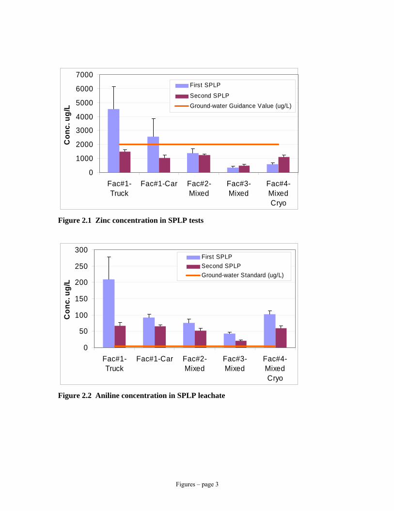
Figures – page 3
0
1000
2000
3000
4000
5000
6000
7000
Fac#1-Truck
Fac#1-Car Fac#2-Mixed
Fac#3-Mixed
Fac#4-MixedCryo
Con
c. u
g/L
First SPLP
Second SPLPGround-water Guidance Value (ug/L)
Figure 2.1 Zinc concentration in SPLP tests
0
50
100
150
200
250
300
Fac#1-Truck
Fac#1-Car Fac#2-Mixed
Fac#3-Mixed
Fac#4-MixedCryo
Con
c. u
g/L
First SPLPSecond SPLPGround-water Standard (ug/L)
Figure 2.2 Aniline concentration in SPLP leachate

Figures – page 4
0
5
10
15
20
25
Fac#1-Truck
Fac#1-Car Fac#2-Mixed
Fac#3-Mixed
Fac#4-Mixed Cryo
Con
c. u
g/L
First SPLP
Second SPLP
Ground-water Standard(ug/L)
Figure 2.3 Phenol concentration in SPLP leachate
0
200
400
600
800
1000
1200
Fac#1-Truck
Fac#1-Car Fac#2-Mixed
Fac#3-Mixed
Fac#4-MixedCryo
Con
c. u
g/L
First SPLPSecond SPLPUnspecified Organic Compound standard (ug/L)
Figure 2.4 Benzothiazole in SPLP leachate
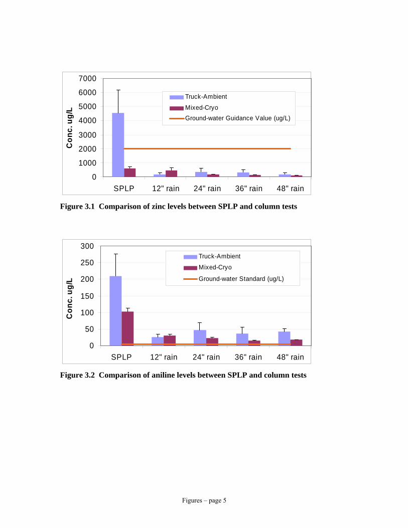
Figures – page 5
0
1000
2000
3000
4000
5000
6000
7000
SPLP 12" rain 24" rain 36" rain 48" rain
Con
c. u
g/L
Truck-Ambient
Mixed-CryoGround-water Guidance Value (ug/L)
Figure 3.1 Comparison of zinc levels between SPLP and column tests
0
50
100
150
200
250
300
SPLP 12" rain 24" rain 36" rain 48" rain
Con
c. u
g/L
Truck-Ambient
Mixed-Cryo
Ground-water Standard (ug/L)
Figure 3.2 Comparison of aniline levels between SPLP and column tests

Figures – page 6
0
5
10
15
20
25
30
SPLP 12" rain 24" rain 36" rain 48" rain
Con
c. u
g/L
Truck-Ambient
Mixed-Cryo
Ground-water Standard (ug/L)
Figure 3.3 Comparison of phenol levels between SPLP and column tests
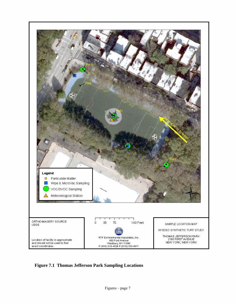
Figures – page 7
Figure 7.1 Thomas Jefferson Park Sampling Locations

Figures – page 8
Figure 7.2 John Mullaly Park Sampling Locations

Figures - page 9
Figure 8.1 Results of airborne particulate monitoring at the Thomas Jefferson Field
0
1
2
3
4
5
6
7
8
9
10
11
12
13
14
15
16
17
18
19
20
17:01
17:03
17:05
17:07
17:09
17:11
17:13
17:15
17:17
17:21
17:23
17:25
17:27
17:29
17:42
17:44
17:46
17:48
17:50
17:56
17:58
18:00
18:02
18:06
18:08
18:10
18:12
18:14
18:17
18:19
18:21
18:23
18:25
Time
PM C
once
ntra
tion
ug/m
3
D099 - Upwind MonitorD921 - Downwind Monitor
PM10 PM10 PM10 PM10PM2.5 PM2.5 PM2.5
Side by Side -
Upwind
Center of Field
Center of Field
Downwind Edge - Center
Downwind Edge - Center
Downwind Edge - Corner
Downwind Edge - Corner
155
Monitor hit by soccer ball
Game in Progress

Figures – page 10
0123456789
1011121314151617181920212223242526
13:3
513
:37
13:3
913
:41
13:4
313
:45
13:4
713
:49
13:5
113
:53
13:5
513
:57
13:5
914
:01
14:0
314
:05
14:0
714
:09
14:1
114
:13
14:1
514
:17
14:1
914
:21
14:2
314
:25
14:2
714
:29
14:3
114
:33
14:3
514
:37
14:3
914
:41
14:4
314
:45
14:4
714
:49
14:5
114
:53
14:5
514
:57
15:0
015
:02
Time
PM C
once
ntra
tion
ug/m
3
D454 - Upwind MonitorD728 - Downwind Monitor
S ide by S ide ‐ Upwind
PM2.5
Figure 8.2 Results of side by side monitoring for airborne particulate monitoring at the upwind location on the John Mullaly Field

Figures – page 11
0123456789
1011121314151617181920212223242526
15:0
3
15:0
5
15:0
7
15:0
9
15:1
1
15:1
3
15:1
7
15:1
9
15:2
1
15:2
3
15:2
5
15:2
7
15:2
8
15:3
0
15:3
2
15:3
4
15:3
6
16:1
4
16:1
6
16:1
8
16:2
016
:22
16:2
4
16:2
6
16:2
8
16:0
2
16:0
4
16:0
6
16:0
8
16:1
0
16:1
2
15:4
8
15:5
0
15:5
2
15:5
4
15:5
6
15:5
8
16:0
0
Time
PM C
once
ntra
tion
ug/m
3
D454 - Upwind MonitorD728 - Downwind Monitor
PM2.5 PM10
Center of Field
Downwind edge - center
Center of Field
Downwind edge - center
Downwind edge - corner
Downwind edge - corner
Figure 8.3 Results of airborne particulate monitoring at the John Mullaly Field

Figures - page 12
60
80
100
120
140
160
180
8/5/
2008
8/7/
2008
8/9/
2008
8/11
/200
8
8/13
/200
8
8/15
/200
8
8/17
/200
8
8/19
/200
8
8/21
/200
8
8/23
/200
8
8/25
/200
8
8/27
/200
8
8/29
/200
8
8/31
/200
8
9/2/
2008
9/4/
2008
9/6/
2008
9/8/
2008
9/10
/200
8
9/12
/200
8
9/14
/200
8
9/16
/200
8
9/18
/200
8
9/20
/200
8
9/22
/200
8
9/24
/200
8
Tem
pera
ture
in F
aren
heit
Center Green TurfCenter White TurfEdge Turf GrassSandBYU Guideline TempAmbient Temp
`
Figure 9.1 Thomas Jefferson field surface temperature measurements by date

Figures – page 13
60
80
100
120
140
160
180
8/5/
2008
8/7/
2008
8/9/
2008
8/11
/200
8
8/13
/200
8
8/15
/200
8
8/17
/200
8
8/19
/200
8
8/21
/200
8
8/23
/200
8
8/25
/200
8
8/27
/200
8
8/29
/200
8
8/31
/200
8
9/2/
2008
9/4/
2008
9/6/
2008
9/8/
2008
9/10
/200
8
9/12
/200
8
9/14
/200
8
9/16
/200
8
9/18
/200
8
9/20
/200
8
9/22
/200
8
9/24
/200
8
Tem
pera
ture
in F
aren
heit
Center TurfEdge Turf Grass Sand BYU Guideline TempAmbient Temp
Figure 9.2 John Mullaly field surface temperature measurements by date

Figures – page 14
60
65
70
75
80
85
90
8/5/
2008
8/7/
2008
8/9/
2008
8/11
/200
8
8/13
/200
8
8/15
/200
8
8/17
/200
8
8/19
/200
8
8/21
/200
8
8/23
/200
8
8/25
/200
8
8/27
/200
8
8/29
/200
8
8/31
/200
8
9/2/
2008
9/4/
2008
9/6/
2008
9/8/
2008
9/10
/200
8
9/12
/200
8
9/14
/200
8
9/16
/200
8
9/18
/200
8
9/20
/200
8
9/22
/200
8
9/24
/200
8
Tem
pera
ture
in F
aren
heit
Center Green Turf Center White TurfEdge Turf GrassSand AAP - "Longer rest, liquids"
AAP - "Limit activities" AAP - "Cancel all activities"
Figure 9.3 Thomas Jefferson field wet bulb globe temperatures by date

Figures – page 15
60
65
70
75
80
85
90
8/5/
2008
8/7/
2008
8/9/
2008
8/11
/200
8
8/13
/200
8
8/15
/200
8
8/17
/200
8
8/19
/200
8
8/21
/200
8
8/23
/200
8
8/25
/200
8
8/27
/200
8
8/29
/200
8
8/31
/200
8
9/2/
2008
9/4/
2008
9/6/
2008
9/8/
2008
9/10
/200
8
9/12
/200
8
9/14
/200
8
9/16
/200
8
9/18
/200
8
9/20
/200
8
9/22
/200
8
9/24
/200
8
Tem
pera
ture
in F
aren
heit
Center Turf Edge Turf Grass Sand AAP - "Longer rest, liquids" AAP - "Limit activities"AAP - "Cancel all activities"
Figure 9.4 John Mullaly field wet bulb globe temperatures by date