an eco-driving advisory system for continuous signalized...
TRANSCRIPT
Research ArticleAn Eco-Driving Advisory System for Continuous SignalizedIntersections by Vehicular Ad Hoc Network
Wei-Hsun Lee and Jiang-Yi Li
Department of Transportation and Communication Management Science National Cheng Kung University No 1University Road Tainan City 701 Taiwan
Correspondence should be addressed to Wei-Hsun Lee leewsmailnckuedutw
Received 20 May 2017 Accepted 15 January 2018 Published 5 March 2018
Academic Editor Mohammad Hamdan
Copyright copy 2018 Wei-Hsun Lee and Jiang-Yi LiThis is an open access article distributed under theCreative CommonsAttributionLicense which permits unrestricted use distribution and reproduction in anymedium provided the originalwork is properly cited
With the vehicular ad hoc network (VANET) technology which support vehicle-to-vehicle (V2V) and vehicle to road side unit(V2RR2V) communications vehicles can preview the intersection signal plan such as signal countdown message In this paperan ecodriving advisory system (EDAS) is proposed to reduce CO2 emissions and energy consumption by letting the vehiclecontinuously pass throughmultiple intersectionswith theminimumpossibilities of stopsWe extend the isolated intersectionmodeltomultiple continuous intersections scenario A hybridmethod combining three strategies includingmaximized throughputmodel(MTM) smooth speedmodel (SSM) andminimized acceleration and deceleration (MinADM) is designed and it is compared withrelated works maximized throughput model (MaxTM) open traffic light control model (OTLCM) and predictive cruise control(PCC)models Some issues for the practical application including safe car following queue clearing and glidingmode are discussedand conquered Simulation results show that the proposed model outperforms OTLCM 251sim812 in the isolated intersectionscenario for the CO2 emissions and 205sim843 in averaged travel time It also performs better than the compared PCC modelin CO2 emissions (199sim312) as well as travel time (245sim359) in the multiple intersections scenario
1 Introduction
Greenhouse gases (GHG) are recognized as the main causeof the global warming with CO2 being the primary GHGemitted through human activities Studies by the IEA [1 2]show that transport was responsible for 23 of world CO2emissions in 2014 as shown in Figure 1(a) Within this thefastest growth in emissions has been from the road transportsector as shown in Figure 1(b) which increased by 64 since1990 and accounted for about three-quarters of transport-related emissions in 2014 [1] In other words encourag-ing environmentally friendly driving practices (eco-drivinghereafter) by eliminating unnecessary vehicle accelerationand braking would reduce fuel consumption and CO2 emis-sions and contribute to slowing down global warming Thedevelopment of eco-driving systems is thus attracting stronginterest from academia vehicle industry and governments
A typical driving trip consists of idling acceleratingcruising and decelerating and the related CO2 emissionsdepend on changes in driver behavior road geometry or
traffic congestion [3] Barth and Boriboonsomsin show thatwhen a vehicle is idling it consumes more fuel and emitsmore exhaust fumes than when it cruises at a steady speed[3] Similarly Frey et al [4] show that accelerating anddecelerating cause more emissions than idling In otherwords avoiding unnecessary engine idling periods and stopsand optimizing driving speedswill reduceCO2 emissions andfuel consumption An eco-driving advisory system (EDAS)which provides smooth driving suggestion according tocurrent traffic dynamics and traffic signal plan can helpdrivers travel in an environmentally friendly manner
With vehicular ad hoc network (VANET) also namedas connected vehicle technology vehicles equipped with anon-board unit (OBU) can communicate with road side units(RSU) by vehicle-to-roadside (V2RR2V) to preview thetraffic signal plans and obtain real-time information such aswaiting queue length and signal countdown message For-ward collision warning (FCW) which can detect the distancerelative to the vehicle ahead facilitates vehicle safety drivingassistance such as adaptive cruise control (ACC) Assuming
HindawiJournal of Advanced TransportationVolume 2018 Article ID 5060481 12 pageshttpsdoiorg10115520185060481
2 Journal of Advanced Transportation
Electricity and heat
42
Transport 23
Industry 19
Residential 6
Services 3
6
OtheLlowast 7
(a) World CO2 emissions by sector
0
1
2
3
4
5
6
7
8
1990 2014
Aviation bunkersMarine bunkersOther transport
Domestic aviationDomestic navigationRoad
N2
(b) CO2 emissions from transport
Figure 1 Statistics on CO2 emissions produced by the IEA [1]
that vehicles are equipped with VANET and FCW OBUcan obtain real-time information and calculate the optimaleco-speed to cross an intersection Our previous work [5]proposed two decision tree based eco-driving suggestionmodels for an isolated signalized intersection using OBUto calculate the best eco-driving speed based on real-timeinformation including the traffic signal countdown messagesand waiting queue length broadcasted by RSU These twomodels are calledMaxTM (maximize throughputmodel) andMinADM (minimize acceleration and deceleration model)simulation results show that MaxTM outperforms MinADMand Open Traffic Light Control Model (OTLCM) [6] being5 to 102 better than MinADM and 13 to 209 betterthanOTLCMwith regard to CO2 emissions in the simulationcases and 8 to 14 better than MinADM and 15 to 231better than OTLCM in the real traffic cases [5]
MaxTM MinADM [5] and OTLCM [6] are applied forthe isolated intersection scenario however in practice vehi-cles may pass a number of intersections when traveling fromorigin to destination In such cases the isolated intersectioneco-driving model may not always be appropriate for usewith multiple intersections since OBU does not acquire thenecessary information from the next RSUs and thus thesemodels cannot provide an optimized speed for the sequentialintersections For example in Figure 2(a) the vehicle maydrive at an unnecessarily high speed if it applies the isolatedEDAS model and it has to stop at the second intersectionas it does not have the traffic signal countdown message forthe next intersection as illustrated in Figure 2(b) With thereal-time information of the traffic signal timing plans ofthe sequential intersections it is possible to design a bettereco-driving model to avoid these energy wasting cases thuslowering fuel consumption and CO2 emissions
In this paper we extend our previous works [5 7] todevelop an EDAS that help drivers to avoid unnecessaryacceleration braking engine idling periods and stops andto optimize the driving speed in a continuous multiple inter-sections scenario Several studies in the literature discuss themultiple intersection scenario Alsabaan et al proposed anEEFGmodel [8] by using decision tree tomeasure the optimalspeed to pass multiple intersectionsThey then improved thisin 2013 [9] by dividing the road region into two parts onepassable and the other unpassable Asadi andVahidi [10] use apredictive cruise control (PCC) algorithm in a mathematicalprogramming model to calculate the most economic cruisespeed without changing the velocity to pass through sequen-tial intersections Similar to the underlying concept of theMaxTM the speed suggested by PCC [10] can be as high asthe free flow speed in order to maximize the throughput inconditions when this is possible The results of their workshow that the proposed model can reduce fuel consumptionby up to 47 compared to the baseline model Katsaroset al [11] proposed GLOSA (Green Light Optimized SpeedAdvisory) which combines GPS information with commonvehicle sensors to obtain more accurate road slope estimateswhich are then used to optimize the fuel consumption of thevehicle thus achieving a 7 reduction in fuel consumptioncomparing to the baseline In summary while a number ofworks have proposed eco-driving advice systems for multipleintersections [8ndash11] they are all insufficient or inefficient forpractical applications due to the following issues not fullyconsidered
(1) Safe Car Following Previous studies either do not considerthe issue of safely following cars [6 8 11] or following acar with a fixed time gap [5] This approach may result
Journal of Advanced Transportation 3
Intersection 1 Intersection 2
Speed limit
V
With multiple intersections infoWithout multiple intersections info
(a) Unnecessarily high speed
With multiple intersections infoWithout multiple intersections info
Intersection 1 Intersection 2
Speed limit
V
(b) Not enough speed
Figure 2 Comparison of the system with and without multiple intersection data
in wasting road capacity at low speed conditions and maycause accidents at high speed ones A dynamic time gapmechanism based on the relative speed and distance of thepreceding vehicle and the host vehicle will increase the usageof road capacity
(2) Queue Clearing When vehicles are stopped by the trafficsignals the time needed for the waiting queue dissipatingcannot be neglected especially when we aim to enable avehicle to pass smoothly through an intersection withoutstopping In related works [6 8ndash11] this issue is not consid-ered so that the model would not be practical for realisticapplications Waiting queue dissipating time which is relatedto the time needed from current time to the last vehiclein the waiting queue passing through the vehicle must beconsidered When the issue of queue clearing is consideredthe resulting eco-driving model will be more accurate and ofgreater practical use
(3) Gliding Mode Only three vehicle moving control modes(acceleration deacceleration andmaintaining current speed)are applied in the traditional models [6 8ndash11] Howevervehicle gliding mode (free from gas pedal) leverages theengine brake to slow the vehicle without additional fuelconsumption thus causing less CO2 emissions than thesecontrol modes When the traffic signal plans are known inadvance vehicles can apply gliding to slow down to thesuggestion speed
In contrast to previous works we take the above issuesinto consideration and propose more realistic and accuratesuggestions with regard to the optimal eco-driving speedSafety is the major concern so that the proposed modelmust follow the safe car following rule speed limit andtraffic signal regulations Two eco-driving strategies areproposed and compared in the continuous intersectionsscenario namely the maximized throughput model (MTM)and smooth speed model (SSM) These are illustrated inFigure 3 in which the green time window upper bounded by119878119867(119894) and lower bounded by 119878119871(119894) (both in red dotted line) are
MTMSSM
V
Intersection 1 Intersection 2 Intersection 3 Intersection 4
SH(i)
SL(i)
Sf
Figure 3 Comparison of two strategies MTM and SSM
first discovered in four continuous signalized intersectionsThe MTM strategy (blue dashed line) keeps the suggestedspeed as high as possible to avoid blocking the followingvehicles thusmaximizing the throughputOn the other handthe SSM strategy (green dashed line) adopts the smoothmoving speed upper bound to avoid unnecessary accelerationand deceleration
The rest of this paper is organized as followsThe assump-tions terminologies and VANET protocol are presented indetail in Section 2The algorithms used inMTM and SSM areproposed in Section 3 Two simulation experiments are thendiscussed in Section 4 including an isolated intersection sce-nario and multiple intersections scenario and the proposedsystemmodels are compared with the PCC [10] OTLCM [6]and MaxTM [5] strategies Finally Section 5 concludes thispaper and presents some directions for future works
2 Eco-Driving System Protocol
Assume that each traffic signal controller is equipped withan RSU and each vehicle is equipped with an OBU whichintegrates a location module (ex GPS) and FCW moduleto detect the speed and distance of the front vehicle Withthese capabilities themain purpose of theOBU is to calculatethe recommended speed (119878119903) and provide driving suggestions(speed upmaintain speedslow downglide) to pass throughas many intersections as possible by considering all thecollected real-time information
4 Journal of Advanced Transportation
VANET single hop range
VANET single hop range
R2R
V2RR2VV2RR2V
Figure 4 Eco-driving advisory system communication schematic
OW2W3 W1 E1 E2 E3
S1
S2
S3
N2
N1
N3
Figure 5 RSU-to-RSU information exchange schematic
The EDAS model is designed on top of the VANETenvironment with V2RR2V communication as illustratedin Figure 4 OBU can collect RSU broadcasted informationbeyond the range of visual contact RSU-to-RSU (R2R) com-munication among the neighborhood RSUs is also includedin the system protocol to exchange the signal timing plan andwaiting queue length information As illustrated in Figure 5every RSU (119877119874) will exchange real-time information withthree neighborhood RSUs (119877119863119894) in each direction includingdata on the waiting queue signal phase timing plan roadlength and traffic conditions
The communication protocol of EDAS is designed asillustrated in Figure 6 which is composed of six steps ofR2R V2R and R2V communication as listed in Table 1 andexplained as below
Step 1 (R2R exchange basic configuration and signal plan)EachRSU as the host RSU itself will exchange its informationwith twelve neighborhoodRSUsThe exchanged informationas shown in (1) is organized as two parts including basicconfiguration and signal plan Basic configuration of anRSU (119877119904) as defined in (1) includes RSU ID (119877119894) location
Table 1
Parameters ValueRoad length (m) 200m 400m 600mTraffic volume (vph) 50 100 200 400 800Traffic signal (sec)(greenred) 3030 4545 6060
Spatial depth Four intersectionsTemporal depth Four cyclesVANET range (m) 200Cruise gliding acceleration minus015ms2
Idle gliding speed (119878min) 2ms
(119883 119884) road length to the next intersection in four directions(119871(119899 119904 119890 119908)) and BSS (basic service set) identification in80211p (SSID) Traffic signal plan and current traffic informa-tion (119877119901) as defined in (2) consisted of cycle time (119879119901) maindirection (north-south) green split (119879119892) current phase (119875119888 0indicates currently signal is green in north-south directionand red in east-west direction and 1 indicates the reversecase) and countdown remaining seconds in north-south andeast-west direction (119877(119899-119904 119890-119908)) With the above definitionsthe R2R data exchange protocol is defined in (3) whichincludes RSU configuration (119877119904) traffic signal plan (119877119901) andtimestamp (119879119904)
119877119904 = 119877119894 119883 119884 119871 (119899 119904 119890 119908) SSID (1)
119877119901 = 119879119901 119879119892 119875119888 119877 (119899-119904 119890-119908) (2)
R2R 119877119904 119877119901 119879119904 (3)
Step 2 (RSUs broadcast synchronized message to OBUs)Each RSU periodically broadcasts message to notify all thevehicles (OBUs) with the range of its transmissions Thesemessages are used to synchronize the OBUs and wake themup if they are not currently in working status The messageformat is shown in (4) including broadcast RSU information(119877119904) and timestamp for time synchronization When anOBU receives one or more RSU broadcasted messages fromdifferent RSUs it first decides which one is the host OBUbased on the relative location and moving direction andcomputes the recommended speed using its current location
Journal of Advanced Transportation 5
Send vehicle info to RSU
Detect host RSU
Start
Receive info from OBU
First RSUs exchange info and send beacon to OBU
Start
Second RSUs exchange info
Send info to OBU Receive info from RSUFCW
Receive info from OBU
First RSUs exchange info and send beacon to OBU
Start
Second RSUs exchange info
Send info to OBU
Step 2 R2V
Step 3 V2R
Step 5 R2V
Step 1 R2R
Step 4 R2R
Step 6
NoYes
Neighborhood RSUs Host RSU OBU
Compute Sr
Figure 6 EDAS communication protocol
speed front vehicle speed and distance (from FCW) and theinformation collected from the host RSU as explained in thenext section
R2V 119877119904 119879119904 (4)
Step 3 (OBUs send information to RSUs) After receivinga synchronized message from the host RSU an OBU willbe in active mode and periodically broadcast informationincluding OBU ID (119874119894) current speed (119878119888) moving direction(119878119889) current acceleration (119860119888) and position (119883 119884) as shownin (5) The OBU also starts to detect the distance and speedof the front car via FCW at the same time
V2R 119874119894 119878119888 119878119889 119860119888 119883 119884 (5)
Step 4 (RSUs exchange dynamic traffic information collectedfromOBUs) AnRSU exchanges dynamic traffic informationwith the neighborhood RSUs in this step calculating thewaiting queue length in each directions by estimating thevehiclesrsquo positions using the collectedOBU information Eachhost RSU updates the neighborhood RSUs array each time anRSU exchange event occurs The exchange message formatis defined in (6) including RSU ID (119877119894) current phase andsignal plan (119877119901) waiting queue length in each direction(119876(119899 119904 119890 119908)) and timestamp 119879119904
R2R 119877119894 119877119901 119876 (119899 119904 119890 119908) 119879119904 (6)
Step 5 (RSUs broadcast dynamic signal message to OBUs)In this step the summarized information of all the RSUsincluding the RSU itself (119877119900) and the twelve neighborhoodRSUs (119877119889119894) organized as an array as shown in (7) isperiodically broadcasted to OBU The information includesthe RSUbasic information (119877119904) traffic signal timing plan (119877119901)
and waiting queue (119876) of host as well as neighborhood RSUsand timestamp 119879119904
R2V 119877119900 [119877119904 119877119901 119876 (119899 119904 119890 119908)] 119877119889119894 [119877119904 119877119901 119876 (119899 119904 119890 119908)] 119879119878 (7)
Step 6 (OBU calculates recommended speed) To calculatethe suggested eco-speed the OBU integrates the collectedRSUs array information broadcasted in Step 5 GPS status(location speed and moving direction) and front vehicleinformation including 119878119901 (speed of front vehicle) and 119863119901(distance to the front vehicle) from FCW The OBU itselfrepeats this step several times based on dynamic GPS statusand FCW information until the new R2V packet arrives
3 Eco-Driving Advisory System
With the EDAS protocol OBU can collect the up-to-dateinformation about upcoming traffic signals including RSUlocations road segment length and traffic signal timing planand real-time traffic information such as the waiting queuelength in each direction for each subsequent RSU and vehicleflow information collected from the host RSUThe goal of theEDAS is to calculate the optimal speed and suggest drivingactions to maximize the possibility of moving through thesubsequent intersections without stopped or waiting behindthe signal By comparing the current moving speed thesuggested speed will be converted into suggested drivingactions such as speed upbrakemaintain speedglide andcan be presented in colored LED bar-liked graphical userinterface
Two critical decisions need to be made before calculatingthe recommended speed (119878119903) based on the collected real-time information and then the three eco-driving strategiesare applied as shown in Figure 7 The suggested driving
6 Journal of Advanced Transportation
Decision 1Can vehicle move passthe current intersectionunder speed limit
Decision 2Traffic flow gtthreshold ()
Process AMaximize throughput
Process BSmooth speed
Process CMinADM
Yes
Yes No
No
Compute Sr
Figure 7 Three strategies are applied in computing 119878119903
Stop
line
Glid
ing
star
ting
Brak
ing
star
ting
posit
ion
Glid
ing
star
ting
posit
ion
at
SSMMTMPCC
posit
ion
atS f
Sf
aver
ageS
H(i)
Smin
Figure 8 Eco-driving strategies comparison of the three models
behaviors of the proposed eco-driving strategies MTM andSSM as well as the comparative eco-driving model PCC [10]are illustrated in Figure 8 The major difference between theMTM SSM and PCC [10] is that the proposed models applyvehicle gliding concept to leverage the engine brake MTMadopts free flow speed (119878119891) and thus applies gliding earlierthan the SSM which adopts smooth speed at upper boundof the speed range (119878119867(119894)) On the other hand PCC [10]has to brake the vehicle in front of the stop line where theaveraged acceleration is much larger than gliding mode Thethree modes two decision criteria and some issues abouteco-driving are discussed in detail below
Decision 1 Isolated or Multi-Intersections Mode The top deci-sion node determines if a vehicle should apply multi-inter-section mode or isolated intersection mode by calculating
whether a vehicle can pass through the current intersectionunder its current conditions with the appropriate speedlimit The decision goes to the left subtree if the answer toDecision-1 is ldquoYesrdquo and otherwise it goes to the right subtreewhere a modified isolated intersection model the simplifiedMinADM will be applied
To find out whether a vehicle can pass the intersectionunder current traffic signal phase119875119888 (green (0) red (1)) phaseremain time (119877(119899-119904 119890-119908)) we can check if the speed neededfor the vehicle to move the distance119863119894 by time period119866119905 fallsinto the speed limit range [119878119891 119878min] as shown in (10) 119866119905 isdefined as the remaining green time if the current signal isgreen and as the remaining red time plus the queue clearingtime (119879119876) if the current signal is red as illustrated in (9)The waiting queue clearance time (119879119876) as defined in (8) isobtained from the literature [12]
119879119876 = 119870sum119896=1
(1003816100381610038161003816119863119896 minus 119863ℎ1003816100381610038161003816) (8)
119866119905 = 119877119894 (119899119904) if 119875119888 = 0119877119894 (119890119908) + 119879119876 if 119875119888 = 1 (9)
Decision 1 = Y if [119863119894119866119905 ] isin [119878119891 119878min]N if [119863119894119866119905 ] notin [119878119891 119878min] (10)
Decision 2 Apply the MTM or SSM Strategy Once Decision-1 is ldquoYrdquo which means the vehicle can pass through cur-rent intersection without stop the multi-intersections modeshould be applied In Decision-2 the EDAS will decidewhether MTM or SSM should be adopted As shown inFigure 3 the MTM strategy tries to maximize the traffic
Journal of Advanced Transportation 7
throughput so that the suggested speed will be as high aspossible while remaining under the speed limit to reduce thepossibility of blocking upstream vehicles The SSM strategyon the other hand tries to minimize the acceleration anddeceleration to keep the vehicle moving as smoothly aspossible The choice between these two strategies will be acompromise solution On peak hours adopting SSM mayresult in more serious traffic congestion as it may block theupstream vehicles so that the number of vehicles stoppedby the signal will rise thus making fuel consumption andCO2 emissions worse On the other hand adopting theMTMstrategy on off-peak hour may increase the fuel consumptiondue to unnecessary acceleration
For this reason we set a compromise factor 120572 as thethreshold to alternate between the throughput oriented andsmooth speed models The value of 120572 is determined by thesensitivity test and once 120572 is determined OBU can decide toapplyMTMor SSM based on the vehicle volume informationcollected from the host RSU
EDAS = MTM if 120572 ge threshold
SSM if 120572 lt threshold (11)
Process A Maximized Throughput Model In the MTM andSSM cases the target of EDAS is to provide the optimaldriving speed suggestion so that vehicles can move throughmultiple sequential intersections without being stopped bya signal In order to maximize throughput and reduce thepossibility of blocking the upstream vehicles MTM suggestsdriving at as high a speed as possible while remaining safeand under constraints such as the speed limit safely followingthe car in front and so on OBU suggests the highest speedunder the calculated speed range to pass the next intersectionwhen the vehicle passes the current intersection By usinghighest speed 119878119867(119894 119895) and lowest speed 119878119871(119894 119895) from (12)which are the speeds needed to pass the 119894th intersection atthe beginning and ending time of the green signal at the 119895thcycle is calculated where 119879119875119894 and 119879119866119894 are the cycle time andgreen time of the 119894th intersection respectively For example119878119867(2 1) indicates the speed needed to drive through thesecond intersection at the first green second of the next signalcycle (119895 = 1) 119878119903(3) indicates the suggested speed to passthe third intersection which is computed by calculating allthe possible speeds in all possible cycles (119895 = 0 to 4) andintersecting this with the speed limitation [119878119891 119878min] Basedon this the highest legal speed in the lowest cycle will be theMTM eco-driving suggested speed (119878119877)
119878119867 (119894 119895) =
119863119894119877119894 (119899119904) + 119895 lowast 119879119866119894 if119875119888 = 0119863119894119877119894 (119890119908) + 119879119876 + 119895 lowast 119879119875119894 if 119875119888 = 1
119878119871 (119894 119895) =
119863119894119877119894 (119899119904) + 119895 lowast 119879119875119894 if119875119888 = 0119863119894119877119894 (119890119908) + 119879119866119894 + 119895 lowast 119879119875119894 if119875119888 = 1
(12)
As illustrated in Algorithm 1 MTM first calculates thespeed needed to pass the 119894th intersection at the 119895th cycle in thefirst green period (119878119867(119894 119895)) or the last green period (119878119871(119894 119895))that is it finds the green band for the vehicle to sequentiallydrive through the intersections without any signal stops Byusing the MTM strategy OBU will choose the highest speedin the legal speed range which is available by intersectingthe calculated speed range ([119878119867(119894 119895) 119878119871(119894 119895)]) with the legalspeed range ([119878119891 119878min]) The119872119886119909119878119877[119894] array in Algorithm 1is applied to keep the calculated highest speed in each cycleIt is initialized as zero and is assigned the calculated speedduring the iterations andwill remain at zero if there is no legalspeed that can be assigned because the intersection of the twospeed ranges is empty The results of the MTM are presentedin the suggested speed array 119878119903[119894] For example the array119878119903 = [60 60 50 0] indicates that the vehicle can continuouslydrive through three intersections without stopping and thesuggested speeds for these intersections will be 60 60 and50 kmhr
Process B Smooth SpeedModel If there is a low volume trafficflow then the MTM strategy may not be energy efficientbecause unnecessary acceleration would not help the vehicleto pass throughmore intersections than the SSM strategyTheSSM suggests a smooth driving speed that passes as manyintersections as possible at a stable speed This enables moreeconomic driving as well as a more comfortable experiencesince it avoids sudden acceleration or deceleration Here weintroduce a parameter 120573 to let the advised speed range from119878119867(119894 119895) to 119878119871(119894 119895) and the recommended speed 119878119903 in SSM canbe obtained from
119878119903 (119894) = 119878119871 (119894 119895) + 120573 lowast (119878119867 (119894 119895) minus 119878119871 (119894 119895)) (13)
Process C Isolated Intersection Model (MinADM) In thisprocess the vehicle condition is that it has to stop by thesignal at the intersection under the current signal phase(either green or red) and there is no need to consider theprobability of blocking any vehicles that are behind itWe thusadopt the minimized acceleration and deceleration model(MinADM) which is simplified from a model proposed inour previous work [5] In this model OBU is only concernedwith maintaining speed and deciding when to begin slowingdownby gliding [5]The recommended speed Sr in thismodelis obtained from (14) and (15)
(1) When the current phase is green
119878119903 = 119878119888 + 119860119892 sdot 119905 if
1198782119888minus2 lowast 119860119892 le 119889119868 le1198782119888minus2 lowast 119860119892119878119888 otherwise
(14)
(2) When the current phase is red
119878119903=
119878119888 + 119860119892 sdot 119905 if1198782119888minus2 lowast 119860119892 le 119889119868 minus 119876 le
1198782119888minus2 lowast 119860119892 + 119863ℎ119878119888 otherwise
(15)
8 Journal of Advanced Transportation
Input119873 number of intersections119872 number of cyclesRSU[119894] RSU array (119863119894 119877119894(119899119904) 119877119894(ew) 119879119866119894 119879119875119894)
Output 119878119903[119894] suggested speed for passing intersections 1 sdot sdot sdot 119873(1) finding out min max speed for passing through 119894th intersection at 119895th cycle(2) for (119894 = 1 119894 lt= 119873 119894++) iterate119873 intersections(3) for (119895 = 0 119895 lt 119872 119895++) iterate119872 cycles 119895 = 0means current cycle(4) if (119875119888 = 0) current signal is green(5) 119878119867(119894 119895) =119863119894(RSU[119894] sdot 119877119899119904 + 119895 lowast RSU[119894] sdot 119879119866) (6) 119878119871(119894 119895) = 119863119894(RSU[119894] sdot 119877119899119904 + 119895 lowast RSU[119894] sdot 119879119875)(7) else current signal is red(8) 119878119867(119894 119895) =119863119894(RSU[119894] sdot 119877119890119908 + RSU[119894] sdot 119879119876 + 119895 lowast RSU[119894] sdot 119879119875)(9) 119878119871(119894 119895) = 119863119894(RSU[119894] sdot 119877119890119908 + RSU[119894] sdot 119879119866 + 119895 lowast RSU[119894] sdot 119879119875)(10) (11) (12) (13) calculate the suggested speed for each intersection 119894(14) for (119894 = 1 119894 lt= 119873 119894++) iterate119873 intersections(15) MaxSR[119894] = 0 initialize suggested speed(16) for (119895 = 0 119895 lt 119872 119895++) iterate119872 cycles to get max legal speed(17) if ((119878119891 lt 119878119871(119894 119895)) continue no solution(18) if (119878119867(119894 119895) le 119878119891) 119878119903[119894] = 119878119867(119894 119895) else 119878119903[119894] = 119878119891(19) if (MaxSR[119894] lt 119878119903[119894])MaxSR[119894] = 119878119903[119894] choose the fastest(20) (21) 119878119903[119894] = 119872119886119909119878119877[119894](22) (23) Output 119878119903[119894]Algorithm 1 MTM eco-driving suggested speed (119878119903)
The Issue of Safely Following Cars In EDAS the top priorityis the issue of safely car following whatever the suggestedspeed is OBU must obey the car following rule to preventthe vehicle from being closer than the safe distance In suchcases OBU will dynamically calculate the suggested speed tomaintain a safe distance from the front vehicle
If the FCW module detects a front vehicle OBU willswitch to car following mode due to safety concerns In thisstudy we apply ISO 15623 [13] to keep a safe distance betweenthe focal vehicle and the one in front Aa shown in (16) thesafe distance (119863119904) can be calculated by the vehiclersquos currentspeed (119878119888) front car current speed (119878119901) average maximumdeceleration of both the vehicles (119860119889) OBU refresh time 119905and additional safe headway space (119863ℎ and in this studywe set this as 1 meter) The suggested safe speed 119878119904 formaintaining the safe distance119863119904 in the car following mode isdefined in (17) which can be inferred by combining Newtonrsquosthree law of motions with (16)
119863119904 = 119878119888 sdot 119905 + (1198781198882 minus 11987811990122119860119889 ) + 119863ℎ (16)
119878119904 = 2119878119901 minus 119878119888 + 119860119901 sdot 119905 minus 2119905 (119863119904 minus 119863119901) (17)
Driving Action Suggestion With the suggested moving speed119878119903 (without a front vehicle) or 119878119904 (with a front vehicle)OBU can suggest appropriate eco-driving actions including
speeding up maintaining current speed gliding (no pressureapplied on the gas pedal) maintaining the safe speed orbraking by comparing the suggested speed (119878119904 or 119878119903) and thevehiclersquos current speed (119878119888)4 Simulation Study and Discussions
Three experiments are designed to evaluate the performanceof the proposed MTM and SSM by comparing then withthree related models In the isolated intersection scenarioMTM is compared with MaxTM [5] and OTLCM [6] In themultiple intersection scenario MTM and SSM are comparedwith MaxTM [5] and PCC [10] The third experiment tests 10real cases collected from local city traffic bureau in isolatedscenario The performance of all the models is evaluated andsimulated using Arena [14] a general simulation softwarewhich is effective in modeling and analyzing processes orflows
To simplify the proposed model and without loss ofgenerality the traffic signal in the yellow (Y) period iscombined with that in the green (G) period and all thered (AR) periods are combined into the red (R) period Theassumptions used in all the simulation experiments are asfollows (1) all the vehicles are with traditional combustionengine hybrid electric vehicle (HEV) and plugin hybridelectric vehicle (PHEV) are not considered in this work (2)each traffic signal is equipped with an RSU and the OBUpenetration rate is 100 (3) there are no lane changes orovertaking (4) drivers always follow the recommend speed
Journal of Advanced Transportation 9
0
50
100
150
200
250
300
50 100 200 400 800 50 100 200 400 800 50 100 200 400 800
OTLCMMaxTMMTM
(kg)
Road length 200 m (VPH) Road length 400 m (VPH) Road length 600 m (VPH)
Figure 9 CO2 emission comparison in isolated intersection case
(5) there is only one type of vehicle (6) all the signal cycletimes and green splits (the fraction of a cycle when thesignal is green) are the same in one simulation and (7)both RSU andOBU adopt the one-hopmessage broadcastingmechanism The simulation parameters are summarized inTable 1TheVANET one-hop communication range is 200mthe road length parameters are 200sim600m the traffic volume(in each direction) parameters range from 50 to 800 vphand the traffic signal green-red period parameters are 30304545 and 6060 For eachOBU four sequential intersectionsare simultaneously considered in the spatial dimension andfour cycles are considered for each RSU in the temporaldimension
To evaluate and compare the CO2 emissions we adoptthe Models for Projecting Energy Consumption and AirPollutants Emissions (MPECAPE) [15] which considersmicroscopic CO2 emissions and was developed by theInstitute of Transportation Ministry Of Transportation andCommunications (MOTC) inTaiwan It is established in 2007by MOTC using emissions data collected from various typesof vehicles considering multiple vehicle driving scenariosincluding on highways and in townships and urban areas
Experiment 1 (isolated intersection scenario) In an isolatedintersection located in the center of four road segments infour directions each road segment has two lanes connectedin two directions one for each directionThe proposedMTMis compared withMaxTM [5] and OTLCM [6] with regard toCO2 emissions and average travel time as shown in Figures 9and 10 respectively The results show that in the case of roadlengths 200m 400m and 600m the CO2 emission of MTMis less than MaxTM [5] and OTLCM [6] models on the casesfrom sparse traffic condition (50 vph) to congested condition(800 vph) The travel time simulation also shows the similarresult MTM has the best performance averaged travel timeand the travel time variability is very stable in all the roadlength and traffic volume combination cases
Experiment 2 (multiple intersections scenario) A cross roadnetwork topology consisting of thirteen intersections asshown in Figure 5 is applied in the experiment The assump-tions and parameters are the same as those in Experiment 1The two proposed strategies MTM and SSM are compared
020406080
100120140160180200
(sec
)
50 100 200 400 800 50 100 200 400 800 50 100 200 400 800
OTLCMMaxTMMTM
Road length 200 m (VPH) Road length 400 m (VPH) Road length 600 m (VPH)
Figure 10 Averaged travel time comparison in isolated intersectioncase
050
100150200250300350
MaxTMPCC
SSMMTM
(kg)
50 100 200 400 800 50 100 200 400 800 50 100 200 400 800Road length 200 m (VPH) Road length 400 m (VPH) Road length 600 m (VPH)
Figure 11 CO2 emission comparison in multiple intersections case
with MaxTM [5] and PCC [10] with regard to CO2 emis-sions and average travel time as shown in Figures 11 to12 respectively In multiple intersections simulation all theperformances of these four models are quite well MTMoutperforms the other three models SSM PCC [10] andMaxTM [5] in both CO2 emissions average travel time Twointerest points are revealed in this experiment First theperformances of PCC [10] and SSM are almost the samedue to the similar strategy and idea behind these models(except the gliding) Second although MaxTM [5] is anisolated model which without the real-time knowledge ofmultiple intersections it performs better than the PCC [10]and SSM This may due to when SSM tries to smoothly passthrough the multiple intersections the green band (rangedfrom 119878119867(119894 119895) to 119878119871(119894 119895)) will be narrower when the numberof previewed intersections increased This will result in thesuggestion speed (119878119903) advised by the SSM being much lessthan theMaxTM [5] which blocks the upstream vehicles andincreases the possibilities of stops by signal for them
Experiment 3 (real data collected from Tainan traffic bureau)In addition to these simulation cases 10 real traffic casesincluding AM and PM peak hours as well as normal hours(as listed inTable 2) collected from theTransportationBureauof Tainan City Government are also simulated The collectedparameters including road length traffic flow volume andtraffic signal plan (green and red splits) are stated in Table 3The proposed MTM is compared with MaxTM [5] and
10 Journal of Advanced Transportation
Table 2 Case definition of the real traffic cases
Case name Duration ClassificationC1 C6 700 to 1200 am HybridC2 C7 1200 to 1700 am NormalC3 C8 700 to 900 am AM peakC4 C8 1700 to 1900 pm PM peakC5 C10 1900 to 2400 pm Night time
Table 3 Sample parameters of the real traffic cases simulation
Case name Time plan offset VD ID Road length Traffic flow Timing plan 119879119866 Timing plan 119879119877C1 Initial V009600 180m 27972 80 s 40 sC2 Initial V009600 180m 38380 80 s 40 sC3 Initial V009600 180m 36085 80 s 40 sC4 Initial V009600 180m 52606 90 s 40 sC4 105min - - - 80 s 40 sC5 Initial V009600 180m 41902 80 s 40 sC5 120min - - - 75 s 45 sC5 195min - - - 55 s 35 sC6 Initial V052370 170m 3125 75 s 45 sC7 Initial V052370 170m 44335 75 s 45 sC8 Initial V052370 170m 39859 75 s 45 sC9 Initial V052370 170m 50754 95 s 35 sC9 105min - - - 75 s 45 sC10 Initial V052370 170m 40151 75 s 45 sC10 195min - - - 63 s 27 s
507090
110130150170190210
MaxTMPCC
SSMMTM
(sec
)
50 100 200 400 800 50 100 200 400 800 50 100 200 400 800Road length 200 m (VPH) Road length 400 m (VPH) Road length 600 m (VPH)
Figure 12 Averaged travel time comparison in multiple intersec-tions case
OTLCM [6] with regard to CO2 emissions and average traveltime as shown in Figures 13 and 14 respectively The resultsshow that the MTM outperforms MaxTM [5] and OTLCM[6] models in CO2 emissions and average travel time on allthe 10 cases
5 Conclusions
WithVANETOBUon the vehicle can collect the informationfrom RSUs and preview the intersection signal plans so thatit can decide the optimal eco-driving speed to pass throughmultiple intersections with the minimum possibilities ofstopsThiswork proposes a hybridmodel that combines three
C1 C2 C3 C4 C5 C6 C7 C8 C9 C10
OTLCMMaxTMMTM
01020304050607080
(kg)
Figure 13 CO2 emission comparison in 10 real traffic cases
strategies including MTM SSM and MinADM to provideeco-driving suggestions With the proposed EDAS the sug-gested driving actions can help vehicles avoid unnecessaryacceleration and braking and unnecessary stops Moreoverseveral practical issues with regard to applying EDAS inthe real world are taken into consideration including a safeand efficient car following mode signal queue clearing timecruise gliding and idle gliding
Traditionally three indexes are applied to measure theperformance of an intersection in traffic management sci-ence including minimizing waiting queue length minimiz-ing vehicle waiting time and maximizing the average cycle
Journal of Advanced Transportation 11
MTM
OTLCMMaxTM
C1 C2 C3 C4 C5 C6 C7 C8 C9 C100
10000
20000
30000
40000
(sec
)
Figure 14 Travel time comparison in 10 real traffic cases
time throughput These indexes are generally consideredto be positively correlated to each other and thus if oneindex improves so will the two others We adopt a strategyof maximizing the average cycle time throughput and thesimulation testing yielded promising results Originally theMTM is designed for multiple intersections cases howeverthe results show that it is 186sim401 better thanMaxTM [5]and 251sim812 better than OTLCM [6] in CO2 emissions166sim477 better than MaxTM [5] and 205sim843better than OTLCM [6] in averaged travel time when MTMis applied to the isolated intersection scenario For themultiple intersections scenario the proposedMTM and SSMoutperformed the PCC [10] model as well as the MaxTM [5]Comparing to PCC [10] MTM is 199sim312 better in CO2emissions and 245sim359 better in travel time
In real applications eco-driving recommendationsdepend heavily on traffic conditions [5] While the maximizethroughput strategy has good performance in congested aswell as normal traffic conditions it may not be suited forthe case of very low traffic flow in off-peak hours since thechance of blocking the rear vehicles is very low In suchconditions the SSM approach should be applied as it mayhave better performance than in the MTM In future workthe traffic congestion threshold (120572) will be studied in moredetail and decided by sensitivity test experiments Moreoverthe smooth speed control parameter (120573) which is appliedto decide the suggested speed in SSM (as shown in (13))can be further studied to acquire the optimal driving speedOnce these issues have been dealt with the MTM and SSMcan be combined into one eco-driving advisory systemthat is more practical for use with continuous signalizedintersections
Notations
119877119894 119877119904 119877119901 RSU ID configuration and signal plan119877119900 119877119889119894 Host RSU 119894th neighborhood RSU indirection 119889119874119894 OBU ID119899 119904 119890 119908 North South East West119899-119904 119890-119908 North and south direction East andwest direction
119883 119884 Longitude and latitude119879119901 Cycle time period119879119892(119899-119904) Green light time period in north-southdirection119879119904 Time stamp119875119888 Current phase (0 = green 1 = Red) in maindirection (north-south)119877(119899-119904 119890-119908) Countdown remaining period119871 Road length (119871119899 119871 119904 119871119890 119871119908)119876119889 Queue length in direction 119889119879119876(119889) Queue dissipating time for direction 119889119878119891 Free flow speed (Or speed limit)119878min Min speed limit119878119903 Recommend speed119878119904 Safety speed for car following119878119888 Current speed119878119901 Front car speed119878119889 Direction119878119867(119894 119895) Pass speed upper limit for 119894th signal at 119895thcycle119878119871(119894 119895) Pass speed bottom limit for 119894th signal at 119895thcycle119860119888 Current acceleration119860119901 Acceleration of the front car119860119892 Cruise gliding deceleration119863119875 Front car distance119863ℎ Minimum discharge headway119863119896 Headway of the 119896th queued vehicle
SSID RSUWi-Fi SSID120572 Traffic congestion threshold120573 SSM control parameter
Conflicts of Interest
The authors declare that there are no conflicts of interestregarding the publication of this paper
Acknowledgments
This work is supported in part by Ministry of Science andTechnology of the Republic of China under Grant no MOST106-2221-E-006-044-
References
[1] IEA CO2 Emissions from Fuel Combustion 2016 IEA 2016[2] IEA (2017) World Energy Outlook 2017 Nov 2017[3] M Barth and K Boriboonsomsin ldquoTraffic congestion and
greenhouse gasesrdquo Access Magazine vol 2-9 2009[4] H C Frey A Unal N M Rouphail and J D Colyar ldquoOn-
roadmeasurement of vehicle tailpipe emissions using a portableinstrumentrdquo Journal of the Air amp Waste Management Associa-tion vol 53 no 8 pp 992ndash1002 2003
[5] W-H Lee Y-C Lai and P-Y Chen ldquoA study on energy savingand CO2 emission reduction on signal countdown extensionby vehicular Ad Hoc networksrdquo IEEE Transactions on VehicularTechnology vol 64 no 3 pp 890ndash900 2015
[6] C Li and S Shimamoto ldquoAn open traffic light control model forreducing vehiclesrsquo CO2 emissions based on ETC vehiclesrdquo IEEE
12 Journal of Advanced Transportation
Transactions on Vehicular Technology vol 61 no 1 pp 97ndash1102012
[7] J-Y Lee A VANET Based ECO-Driving Advisory System forReducing Fuel Consumption and CO2 Emissions on SignalizedMulti-intersections [Master thesis] National Cheng Kung Uni-versity 2014
[8] M Alsabaan K Naik T Khalifa and A Nayak ldquoVehicularnetworks for reduction of fuel consumption andCO2 emissionrdquoin Proceedings of the 8th IEEE International Conference onIndustrial Informatics INDIN 2010 pp 671ndash676 jpn July 2010
[9] M Alsabaan K Naik and T Khalifa ldquoOptimization of fuel costand emissions using V2V communicationsrdquo IEEE Transactionson Intelligent Transportation Systems vol 14 no 3 pp 1449ndash1461 2013
[10] B Asadi and A Vahidi ldquoPredictive cruise control utilizingupcoming traffic signal information for improving fuel econ-omy and reducing trip timerdquo IEEE Transactions on ControlSystems Technology vol 19 no 3 pp 707ndash714 2011
[11] K Katsaros R Kernchen M Dianati and D Rieck ldquoPer-formance study of a Green Light Optimized Speed Advisory(GLOSA) application using an integrated cooperative ITSsimulation platformrdquo in Proceedings of the 7th InternationalWireless Communications and Mobile Computing Conference(IWCMC rsquo11) pp 918ndash923 Istanbul Turkey July 2011
[12] J A Bonneson ldquoChange intervals and lost time at single-point urban interchangesrdquo Highway Capacity and Traffic Flow(Transportation Research Record) 32 1993
[13] ISO (2013) Intelligent transport systems ndash Forward vehiclecollision warning systems -Performance requirements and testprocedures ISO156232013
[14] W Kelton R Sadowski and N Zupick Simulation with Arena6e McGraw-Hill 6e 2015
[15] K Lin Integrating the Applications of Sustainable TransportationPlanning Model and Models for Projecting Energy Consumptionand Air Pollutants Emissions Institute of Transportation Min-istry of Transportation and Communications 2010
International Journal of
AerospaceEngineeringHindawiwwwhindawicom Volume 2018
RoboticsJournal of
Hindawiwwwhindawicom Volume 2018
Hindawiwwwhindawicom Volume 2018
Active and Passive Electronic Components
VLSI Design
Hindawiwwwhindawicom Volume 2018
Hindawiwwwhindawicom Volume 2018
Shock and Vibration
Hindawiwwwhindawicom Volume 2018
Civil EngineeringAdvances in
Acoustics and VibrationAdvances in
Hindawiwwwhindawicom Volume 2018
Hindawiwwwhindawicom Volume 2018
Electrical and Computer Engineering
Journal of
Advances inOptoElectronics
Hindawiwwwhindawicom
Volume 2018
Hindawi Publishing Corporation httpwwwhindawicom Volume 2013Hindawiwwwhindawicom
The Scientific World Journal
Volume 2018
Control Scienceand Engineering
Journal of
Hindawiwwwhindawicom Volume 2018
Hindawiwwwhindawicom
Journal ofEngineeringVolume 2018
SensorsJournal of
Hindawiwwwhindawicom Volume 2018
International Journal of
RotatingMachinery
Hindawiwwwhindawicom Volume 2018
Modelling ampSimulationin EngineeringHindawiwwwhindawicom Volume 2018
Hindawiwwwhindawicom Volume 2018
Chemical EngineeringInternational Journal of Antennas and
Propagation
International Journal of
Hindawiwwwhindawicom Volume 2018
Hindawiwwwhindawicom Volume 2018
Navigation and Observation
International Journal of
Hindawi
wwwhindawicom Volume 2018
Advances in
Multimedia
Submit your manuscripts atwwwhindawicom
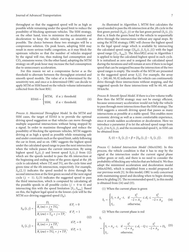

International Journal of
AerospaceEngineeringHindawiwwwhindawicom Volume 2018
RoboticsJournal of
Hindawiwwwhindawicom Volume 2018
Hindawiwwwhindawicom Volume 2018
Active and Passive Electronic Components
VLSI Design
Hindawiwwwhindawicom Volume 2018
Hindawiwwwhindawicom Volume 2018
Shock and Vibration
Hindawiwwwhindawicom Volume 2018
Civil EngineeringAdvances in
Acoustics and VibrationAdvances in
Hindawiwwwhindawicom Volume 2018
Hindawiwwwhindawicom Volume 2018
Electrical and Computer Engineering
Journal of
Advances inOptoElectronics
Hindawiwwwhindawicom
Volume 2018
Hindawi Publishing Corporation httpwwwhindawicom Volume 2013Hindawiwwwhindawicom
The Scientific World Journal
Volume 2018
Control Scienceand Engineering
Journal of
Hindawiwwwhindawicom Volume 2018
Hindawiwwwhindawicom
Journal ofEngineeringVolume 2018
SensorsJournal of
Hindawiwwwhindawicom Volume 2018
International Journal of
RotatingMachinery
Hindawiwwwhindawicom Volume 2018
Modelling ampSimulationin EngineeringHindawiwwwhindawicom Volume 2018
Hindawiwwwhindawicom Volume 2018
Chemical EngineeringInternational Journal of Antennas and
Propagation
International Journal of
Hindawiwwwhindawicom Volume 2018
Hindawiwwwhindawicom Volume 2018
Navigation and Observation
International Journal of
Hindawi
wwwhindawicom Volume 2018
Advances in
Multimedia
Submit your manuscripts atwwwhindawicom