An Educational Kit Based on a Modular SiliconPhotomultiplier System

Valentina Arosio, Massimo Caccia, Valery Chmill, Amedeo Ebolese, Marco Locatelli, Alexander Martemiyanov,Maura Pieracci, Fabio Risigo, Romualdo Santoro and Carlo Tintori

Abstract—Silicon Photo-Multipliers (SiPM) are state of the artlight detectors with unprecedented single photon sensitivity andphoton number resolving capability, representing a breakthroughin several fundamental and applied Science domains. An educa-tional experiment based on a SiPM set-up is proposed in thisarticle, guiding the student towards a comprehensive knowledgeof this sensor technology while experiencing the quantum natureof light and exploring the statistical properties of the light pulsesemitted by a LED.

Keywords—Silicon Photo-Multipliers, Photon Statistics, Educa-tional Apparatus

I. INTRODUCTION

EXPLORING the quantum nature of phenomena is oneof the most exciting experiences a physics student can

live. What is being proposed here has to do with light bullets,bunches of photons emitted in a few nanoseconds by anultra-fast LED and sensed by a state-of-the-art detector, aSilicon Photo-Multiplier (hereafter, SiPM). SiPM can countthe number of impacting photons, shot by shot, opening upthe possibility to apply basic skills in probability and statisticswhile playing with light quanta. After an introduction tothe SiPM sensor technology (Section II), the basics of thestatistical properties of the random process of light emissionand the sensor related effects are introduced (Section III).The experimental and data analysis techniques are describedin Section IV, while results and discussions are reported inSection V.

II. COUNTING PHOTONS

SiPMs are cutting edge light detectors essentially consistingof a matrix of photodiodes with a common output and densitiesup to 104/mm2. Each diode is operated in a limited Geiger-Muller regime in order to achieve gains at the level of≈ 106 and guarantee an extremely high homogeneity in thecell-to-cell response. Subject to the high electric field inthe depletion zone, initial charge carriers generated by anabsorbed photon or by thermal effects trigger an exponentialcharge multiplication by impact ionization, till when thecurrent spike across the quenching resistance induces a dropin the operating voltage, stopping the process [1], [3], [4].

M. Caccia, V. Chmill, A. Ebolese, A. Martemiyanov, F. Risigo andR. Santoro are with the Dipartimento di Scienza e Alta Tecnologia,Universita’ degli Studi dell’Insubria, 22100, Como, Italy (e-mail: mas-simo.caccia@uninsubria.it).

M. Locatelli, M. Pieracci and C. Tintori are with the CAEN S.p.A., 55049,Viareggio, Italy (e-mail: m.locatelli@caen.it).

SiPM can be seen as a collection of binary cells, providingaltogether an information about the intensity of the incominglight by counting the number of fired cells.

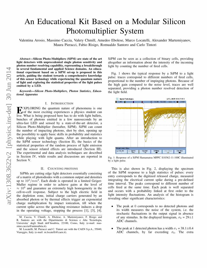
Fig. 1 shows the typical response by a SiPM to a lightpulse: traces correspond to different numbers of fired cells,proportional to the number of impinging photons. Because ofthe high gain compared to the noise level, traces are wellseparated, providing a photon number resolved detection ofthe light field.

Fig. 1: Response of a SiPM Hamamatsu MPPC S10362-11-100C illuminatedby a light pulse.

This is also shown in Fig. 2, displaying the spectrumof the SiPM response to a high statistics of pulses: everyentry corresponds to the digitized released charge, measuredintegrating the electrical current spike during a pre-definedtime interval. The peaks correspond to different number ofcells fired at the same time. Each peak is well separatedand occurs with a probability linked at first order to thelight intensity fluctuations. An analysis of the histogram isrevealing other significant characteristics:

• The peak at 0 corresponds to no detected photons andits width measures the noise of the system, i.e. thestochastic fluctuations in the output signal in absenceof any stimulus. In the displayed histogram, σ0 = 29±1ADC channels.

• The peak at 1 detected photon has a width σ1 = 38.1±0.4ADC channels, by far exceeding σ0. The extra

arX

iv:1

308.

3622

v2 [

phys

ics.

ins-

det]

30

Jun

2014

0 500 1000 1500 2000 2500 3000 3500 40000

300

600

900

1200

1500

1800

Channel [ADC]

Ent

ries

Fig. 2: Photoelectron spectrum probing a LED source measured with a Hama-matsu MPPC S10362-11-100C at a bias voltage of 70.3V and temperature of25oC.

contribution may be related to the fact that not all ofthe cells were born equal. In SiPM the homogeneity ofthe response is quite high [5], [6], however, since firedcells are randomly distributed in the detector sensitivearea residual differences in the gain become evidentbroadening the peak.

• As a consequence the peak width is increasing withthe number N of fired cells with a growth expected tofollow a

√N law, eventually limiting the maximum

number M of resolved peaks.

0 −10 −20 −30 −40 −50 −60 −7010

0

102

104

106

Threshold [mV]

DC

R [H

z]

Fig. 3: Measurement of the DCR of the SiPM performed at 25oC.

The detector working conditions can be optimized to maxi-mize M, properly tuning the bias voltage Vbias and balancingcompeting effects. On one hand, the peak-to-peak distance islinked to the single cell gain and it is expected to grow linearlywith the over-voltage as:

Gain =C ∆V

qe, (1)

where ∆V = Vbias − VBreakdown, C is the diode capacitanceof the single cell and qe the electron charge [3]. Effectsbroadening the peaks may grow faster dumping the expectedresolution. Among these effects it is worth mentioning DarkCounts, Optical Cross-Talk and After-Pulsing:

• Free charge carriers may also be thermally generated.Results are spurious avalanches (Dark Counts) occurring

randomly and independently from the illumination field.The Dark Count Rate (DCR) does depend from severalfactors: substrate, processing technology, sensor designand operating temperature [4]. The over-voltage has animpact since the junction thickness volume grows withit together with the triggering probability, namely theprobability that a charge carrier develops an avalanche[4], [5]. The DCR can be measured in different ways.A Stair Case Plot is presented in Fig. 3 where theoutput from a sensor is compared to the threshold ofa discriminator and the rate with which the thresholdis exceeded is counted. A typical DCR is about0.5 MHz/mm2.

• Dark Counts may be considered as statistically inde-pendent. However, optical photons developed duringan avalanche have been shown to trigger secondaryavalanches [4] involving more than one cell into spuriouspulses. This phenomenon is named Optical Cross-Talk(OCT). The OCT is affected by the sensor technology[4], [7], [8], [9] and strongly depends on the biasvoltage increasing the triggering probability and thegain forming the optical photon burst. The OCT can bemeasured by the ratio of the Dark Counts frequenciesfor pulses exceeding the 0.5 and 1.5 levels of the singlecell amplitude, namely:

OCT =ν1.5pe

ν0.5pe. (2)

The OCT typically ranges between 10% and 20% [5],[9], [10].

• Charge carriers from an initial avalanche may betrapped by impurities and released at later stageresulting in delayed avalanches named After-Pulses. Forthe detectors in use here, an After-Pulse rate at aboutthe 25% level has been reported for an overvoltage∆V = 1 V , with a linear dependence on Vbias and atwo-component exponential decay time of 15 ns and80 ns [5].

Dark Counts, Optical Cross-Talk and After-Pulses occurstochastically and introduce fluctuations in the multiplicationprocess that contribute to broaden the peaks in the spectrum.An exhaustive study of this effect, also known as Excess NoiseFactor (ENF), exceeds the goals of this work and will notbe addressed here (see for example [3], [6], [8] and [12]).However, the resolving power that will be introduced in thefollowing may be considered a figure of merit accounting forthe ENF and measuring the ability to resolve the number ofdetected photons.

III. PHOTON COUNTING STATISTICS

Spontaneous emission of light results from random decaysof excited atoms. Occurrences may be considered statisticallyindependent, with a decay probability within a time interval

∆t proportional to ∆t itself. Being so, the statistics of thenumber of photons emitted within a finite time interval T isexpected to be Poissonian, namely:

Pn,ph =λne−λ

n!, (3)

where λ is the mean number of emitted photons.The detection of the incoming photons has a stochastic

nature as well, at the simplest possible order governed by thePhoton Detection Probability (PDE) η, resulting in a Binomialprobability to detect d photons out of n:

Bd,n(η) =

(nd

)ηd(1− η)n−d . (4)

As a consequence, the distribution Pd,el of the number ofdetected photons is linked to the distribution Pn,ph of thenumber of generated photons by

Pd,el =

∞∑n=d

Bd,n(η)Pn,ph . (5)

However, the photon statistics is preserved and Pd,el isactually a Poissonian distribution of mean value µ = λη[9], [10]. For the sake of completeness, the demonstration isreported in Appendix A.

Detector effects (especially OCT and After-Pulses) canactually modify the original photo-electron probability densityfunction, leading to significant deviations from a pure Poissondistribution. Following [9] and [10], OCT can be accountedfor by a parameter εXT , corresponding to the probability of anavalanche to trigger a secondary cell. The probability densityfunction of the number of fired cells, the random discretevariable m, can be written at first order as:

P ⊗B =

floor(m/2)∑k=0

Bk,m−k(εXT )Pm−k(µ), (6)

where floor rounds m/2 to the nearest lower integer andBk,m−k(εXT ) is the binomial probability for m − k cellsfired by a photon to generate k extra hit by OCT. P ⊗ Bis characterized by a mean value and variance expressed as:

mP⊗B = µ(1 + εXT ) σ2P⊗B = µ(1 + εXT ). (7)

In order to perform a more refined analysis, the probabilitydensity function of the total number of detected pulses canbe calculated taking into account higher order effects [13].The result is achieved by assuming that every primary eventmay produce a single infinite chain of secondary pulses withthe same probability εXT . Neglecting the probability for anevent to trigger more than one cell, the number of secondaryhits, described by the random discrete variable k, follows ageometric distribution with parameter εXT :

Gk(εXT ) = εXTk(1− εXT ) for k = 0, 1, 2, 3.... (8)

The number of primary detected pulses is denoted by therandom discrete variable d and belongs to a Poisson distribu-tion with mean value µ. As a consequence, the total numberof detected pulses m represents a compound Poisson processgiven by:

m =

d∑i=1

(1 + ki). (9)

Then, the probability density function of m is expressed asa compound Poisson distribution:

P ⊗G =e−µ

∑mi=0Bi,mµ

i(1− εXT )iεXTm−i

m!, (10)

where

Bi,m =

1 if i = 0 and m = 0

0 if i = 0 and m > 0m!(m−1)!

i!(i−1)!(m−i)! otherwise

The mean value and the variance of the distribution arerespectively given by:

mP⊗G =µ

1− εXTσ2P⊗G =

µ(1 + εXT )

(1− εXT )2. (11)

These relations can be calculated referring to the definitionof the probability generating function and exploiting its fea-tures [13]. The full demonstration is available in Appendix B.

IV. EXPERIMENTAL TECHNIQUES

In this section the experimental set-up and the analysismethods are presented. The optimization of the working pointof a SiPM is addressed together with the recorded spectrumanalysis technique.

Fig. 4: Schematic layout of the experimental set-up.

A. Set-up and measurementsThe experimental set-up is based on the CAEN Silicon

Photomultiplier Kit. The modular plug and play systemcontains:

• The Two channel SP5600 CAEN Power Supply andthree-stage Amplification Unit (PSAU) [14], with SiPM

embedding head unit. The PSAU integrates a leadingedge discriminator per channel and coincidence logic.

• The two channels DT5720A CAEN Desktop Digitizer,sampling the signal at 250 MS/s over a 12 bit dynamicrange. The available firmware enables the possibilityto perform charge Integration (DPP-CI), pulse shapediscrimination (DPP-PSD) and advanced triggering [15].

• The ultra-fast LED (SP5601 [16]) driver emittingpulses at 400 nm with FWHM of 14 nm. Pulses arecharacterized by an exponential time distribution of theemitted photons with a rising edge at sub-nanosecondlevel and a trailing edge with τ ≈ 5 ns. The driver isalso providing a synchronization signal in NIM standard.

In the current experiments the SiPM that was used is a MultiPixel Photon Counter (MPCC) S10362-11-100C produced byHAMAMATSU Photonics1 (see Table I).

TABLE I: Main characteristics of the SiPM sensor (Hamamatsu MPPCS10362-11-100C) at a temperature of 25oC

Number of Cells: 100Area: 1× 1mm2

Diode Dimension: 100 µm × 100 µmBreakdown Voltage: 69.2VDCR: 600 kHz at 70.3VOCT: 20% at 70.3VGain: 3.3× 106 at 70.3VPDE (λ = 440nm): 75% at 70.3V

The block diagram of the experimental set-up is presentedin Fig.4 with light pulses conveyed to the SiPM sensor by anoptical fiber.

The area of the digitized signal is retained as a figureproportional to the total charge generated by the SiPM inresponse to the impacting photons. The integration window(or gate) is adjusted to match the signal development and itis synchronized to the LED driver pulsing frequency.

The proposed experimental activities start with the optimalsetting of the sensor bias voltage, defined maximizing theresolving power defined as:

R =∆pp

σgain, (12)

where ∆pp is the peak-to-peak distance in the spectrum andσgain accounts for the single cell gain fluctuations:

σgain = (σ21 − σ2

0)1/2, (13)

being σ0,1 the standard deviations of the 0- and 1-photoelectron peaks [17]. R is a figure of merit measuringthe capability to resolve neighboring peaks in the spectrum. In

1http://www.hamamatsu.com/.

fact, following the Sparrow criterion [18] according to whichtwo peaks are no longer resolved as long as the dip half waybetween them ceases to be visible in the superposed curves,the maximum number Nmax of identified peaks is given by:

Nmax <R2

4, (14)

where it has been assumed the width of the peaks to growas the squared root of the number of cells (as confirmed bythe data reported in Fig. 5).

0 2 4 6 8 10 12 14 160

2000

4000

6000

8000

10000

12000

14000

N (Peak Number)

σ2 N

Fig. 5: Peaks width for the spectrum Fig.2 by a multi-Gaussian fit. The dashlines represent the 95% C.L. for the fit, shown with the solid line. The circlesindicate the outliers.

The outliers, the data points that are statistically inconsistentwith the rest of the data, are identified with the Thompson Taumethod [19] and discarded.

A typical plot of the resolving power versus the bias voltageis presented in Fig. 6. The optimal biasing value corresponds tothe maximum resolution in the plot and it is used as a workingpoint. After the sensor calibration, spectra for different lightintensities are recorded and analyzed as reported below.

70.2 70.3 70.4 70.5 70.60

5

10

15

20

Bias [V]

R

Fig. 6: Scan of the resolution power R as a function of the bias voltage atfixed temperature (25oC) and light intensity. The working point is given by apolynomial fit and equal to 70.28 V .

TABLE II: Acquisition parameters for the reference run presented in this work.

Vbias[V] GateWidth [ns] Trigger frequency [kHz] Temperature [C]

70.3 300 100 25.0

B. Multi-peak spectrum analysisSpectra recorded in response to photons impacting on the

sensor can be seen as a superposition of Gaussians, each

corresponding to a well defined number of fired cells. Thekey point in the analysis technique is the estimation of thearea underneath every peak, allowing the reconstruction of theprobability density functions.

Initially, areas can be estimated by a Pick&Play (hereafter,P&P) procedure on the spectrum. In fact, a binned Gaussiandistribution of Npk events may be written as:

yi = y(xi) = ymaxe− (xi−x0)2

2σ2 , (15)

where y(xi) is the number of events in the bin centeredon xi and ymax is the peak value, measured in x0. Sinceymax = Npk/(σ

√2π), knowing the content of the bin

centered in x0 and estimating σ leads to Npk. The standarddeviation can also be calculated in a simple way by the FullWidth at Half Maximum (FWHM ), obtained searching forthe position of the bins with a content equals to ymax/2and presuming that FWHM = 2.355 × σ. Advantages andlimitations of this method are quite obvious: its applicabilityis straightforward and essentially requires no tool beyonda Graphical User’s Interface (GUI) for the control of theset-up; on the other hand, it can be applied only to peakswith a limited overlap and uncertainties can only be obtainedby repeating the experiment. In order to overcome theselimitations, a Multi-Gaussian Fit (MGF) procedure wasimplemented in MATLAB to analyze the full spectrum,according to the following work flow:

• Initialization. Robustness and efficiency of minimiza-tion algorithms is guaranteed by having an educatedguess of the parameter values and by defining boundariesin the parameter variation, a procedure increasinglyimportant as the number of parameters grow. Initialvalues are provided in an iterative procedure:

◦ The user is required to identify by pointing &clicking on the spectrum the peak values and theirposition for 3 neighboring Gaussians, fitted toimprove the estimate.

◦ Initial values for every Gaussian are estimatedby relying on the peak-to-peak distance from theprevious step, presuming the signal from the 0-cellpeak to be centered in the origin of the horizontalscale and assuming the standard deviation growsas the squared root of the number of cells.

• Fit. Spectra are fitted to a superposition of Gaussianswith a non-linear χ2 minimization algorithm presumingbinomial errors in the content of every bin. The mostrobust convergence over a large number of tests andconditions have been empirically found bounding pa-rameters to vary within 20% of the initial value for thepeak position, 30% for the area and 50% for the standarddeviation.

V. RESULTS AND DISCUSSIONS.Exemplary spectra for three light intensities were recorded

and the raw data distributions are shown in Fig. 7, wherethe horizontal scale in ADC channels measures the integratedcharge in a pre-defined gate. In the following, the analysissteps are detailed for the distribution corresponding to thehighest mean photon number, hereafter identified as the Refer-ence Spectrum. Remaining spectra will be used to assess therobustness of the approach and the validity of the model, withthe results summarized at the end of the section.

−200 0 200 400 600 800 1000 12000

400

800

1200

1600

2000

2400

2800

Channel [ADC]

Ent

ries

RUN1

−200 0 200 400 600 800 1000 1200 1400 16000

500

1000

1500

Channel [ADC]

Ent

ries

RUN2

0 500 1000 1500 2000 2500 3000 3500 40000

200

400

600

800

1000

1200

1400

1600

1800

Channel [ADC]

Ent

ries

REFERENCE SPECTRUM

Fig. 7: Exemplary spectra. The mean number µMI of photo-electrons ismeasured to be 1.080±0.002 (RUN1), 1.994±0.003 (RUN2) and 7.81±0.01(Reference Spectrum).

Spectra are seen as a superposition of Gaussians, withparameters estimated according to the methods introduced inSection IV. The outcome of the procedures for the ReferenceSpectrum is reported in Table III for the P&P and the MGFprocedures. For the former, uncertainties in the estimatedparameters are the standard deviations from five data setsacquired in identical conditions while for the latter errors resultfrom the fitting procedure (Fig. 8).

The characteristics of the experimental distribution caninitially be studied referring to the mean number of fired cells.A Model Independent (MI) estimate is provided by:

µMI =ADC

∆pp

, (16)

where

ADC =ΣiyiADCi

Σiyi(17)

is the mean value of the experimental distribution (being yithe number of events for the ith bin) and ∆pp is the meanpeak-to-peak distance, defining the gauge to convert values inADC channels to number of cells.

TABLE III: Peak position, width and experimental probability of having Nphoto-electrons from the Pick&Play (P&P) procedure, compared to the resultsfrom the Multi-Gaussian Fit (MGF). The results are for the reference spectrum.

PeakPosition[ADC] PeakWidth[ADC] Exp. Probability

N P&P MGF P&P MGF P&P MGF

0 3± 1 2.1± 0.9 22± 1 21.7± 0.8 0.092± 0.006 0.09± 0.011 220± 1 220.1± 0.4 25± 1 27.3± 0.3 0.53± 0.02 0.56± 0.012 427± 1 428.0± 0.3 30± 1 31.5± 0.2 1.75± 0.06 1.86± 0.023 635± 1 633.6± 0.2 32± 1 36.0± 0.2 3.8± 0.1 4.17± 0.024 838± 2 837.5± 0.2 38± 1 40.5± 0.2 7.0± 0.2 7.21± 0.045 1044± 2 1041.3± 0.2 41± 1 44.7± 0.2 9.9± 0.2 10.30± 0.046 1247± 2 1243.7± 0.2 45± 1 48.2± 0.2 12.2± 0.3 12.67± 0.057 1449± 3 1445.6± 0.2 50± 3 51.9± 0.3 13.4± 0.8 13.43± 0.068 1650± 4 1645.8± 0.3 57± 2 54.8± 0.4 13.3± 0.5 12.71± 0.079 1853± 4 1846.4± 0.4 67± 2 59.5± 0.6 12.9± 0.4 11.2± 0.110 −− 2046.5± 0.6 −− 62.0± 0.9 −− 8.7± 0.111 −− 2245± 1 −− 66± 2 −− 6.6± 0.212 −− 2445± 1 −− 68± 2 −− 4.4± 0.213 −− 2632± 2 −− 65± 3 −− 2.4± 0.1

0 500 1000 1500 2000 2500 3000 3500 40000

200

400

600

800

1000

1200

1400

1600

1800

Channel [ADC]

Ent

ries

χ2/d.o.f = 1.9

Fig. 8: Outcome of the MGF procedure. Individual Gaussians are in red,while their superposition is displayed in green. The χ2/d.o.f. measures thefit quality.

The value of µMI can be compared to what is estimatedpresuming a pure Poissonian behaviour and referring to theprobability P (0) of having no fired cell when the expectedaverage value is µZP , where ZP stands for Zero Peak:

µZP = −ln(P (0)) = −ln(A0

Atot

), (18)

being A0 the area underneath the first peak of the spectrumand Atot the total number of recorded events. Results areshown in Table IV.

TABLE IV: Estimates of the mean number of fired cells by the averagevalue of the experimental distribution and from the probability of havingnone, assuming an underlying Poissonian distribution. Errors result from theuncertainties in the peak-to-peak distance and in the area of the zero-cell peak.

µMI µZP

P&P 7.6 ± 0.3 6.99 ± 0.06

MGF 7.81 ± 0.01 7.08 ± 0.03

The P&P procedure shows a good compatibility with thehypothesis, while the MGF procedure, due to the smallererrors, presents an evident discrepancy.

The question can be further investigated considering thefull distribution and comparing the experimental probabilitydensity function with the assumed model distribution by a χ2

test, where:

χ2 =

Npeaks−1∑k=0

wk × (Aobs,k −Amodel,k)2, (19)

being Aobs,k the number of events in the kth peak of thedistribution, Amodel,k the corresponding number estimatedfrom the reference model and wk the weights accounting forthe uncertainties in the content of every bin. Presuming aPoissonian distribution with mean value µMI , the returnedvalues of the χ2/d.o.f. are ≈ 20 for the P&P procedure and≈ 300 for the MGF . The χ2/d.o.f. values, even assuming µas a free parameter, exceeds the 99% C.L. for both methodsconfirming that the experimental distribution may not beadequately described by a pure Poissonian model.

As a further step, the spectra were compared to the P ⊗Gdistribution model introduced in Section III, Eq. 10, where theactual number of fired cells results from avalanches triggeredby the incoming photons and by the optical cross-talk.The optimal values of the model parameters, namely thecross-talk probability εXT and the mean value µ of thedistribution of cells fired by photons, are determined by agrid search according to the following iterative procedure [20] :

• the χ2/d.o.f. surface, henceforth referred to as Σ, issliced with planes orthogonal to the εXT dimension, atvalues εXT changed with constant step;

• in each slice, the minimum of the Σ(εXT , µ)) curveis searched and the value µmin,0 corresponding to theminimum is identified;

• the Σ(εXT , µmin,0) curve is scanned and the positionε∗XT of the minimum is identified by a local parabolic

fit, to overcome the limitations by the choice of thestep in the grid;

• the procedure is repeated for Σ(ε∗XT , µ) vs µ, leadingto the determination of the minimum in µ∗.

This method leads to estimate the optimal parameters µ∗and ε∗XT by the minimization of the χ2/d.o.f. surface for thetwo variables µ and εXT independently. The surface Σ andthe Σ(ε∗XT , µ) and Σ(εXT , µ

∗) curves are shown in Fig. 9.Uncertainties are calculated assuming a parabolic shape of theχ2/d.o.f. curves, leading to variances estimated by the inverseof the coefficient of the quadratic term [20], [21]. The resultsfor the reference spectrum are µ∗ = 7.06 ± 0.02 and ε∗XT =0.090± 0.004.

0

0.1

0.2

6.86.977.17.27.30

5

10

15

20

εXT

µ

χ2 /dof

0.07 0.08 0.09 0.1 0.110.110

2

4

6

8

10

12

14

16

18

20

εXT

χ2 /dof

7 7.05 7.1 7.150

2

4

6

8

10

12

14

16

18

20

µ

χ2 /dof

Fig. 9: χ2/d.o.f. surface (top panel) and parabolic behavior nearby itsminimum (bottom).

In order to account for the two-parameter correlation inthe calculation of the uncertainties, it is worth to referring tothe confidence region of the joint probability distribution [22][23]. When the parameters are estimated minimizing the χ2

distribution, confidence levels correspond to regions definedby iso-χ2 curves. For two parameters, the region assumes anelliptic shape around the Σ minimum, χ2

min. The Σ contourat the constant value of χ2

min + 1 plays a crucial role due toits specific properties. In fact, the resulting ellipse contains∼ 38.5% of the joint parameter probability distribution and

its projections represent the ∼ 68.3% of confidence intervalfor each parameter (σ1 and σ2). In addition, the correlation ρamong the parameters may be written as:

ρ =σ2

1 − σ22

2σ1σ2tan 2θ, (20)

where θ represents the counter-clockwise rotation angle of theellipse. The detailed demonstration is reported in Appendix C.

In this specific case, the χ2min value is determined evaluating

the χ2/d.o.f. surface at the point of coordinates (µ∗, ε∗XT )while the Σ contour at χ2

min + 1 is shown in Fig.10 (blackcrosses). The fit curve (red line) returns the value of the ellipsecenter (µ0,ε0XT ) (black circle). The projections of the ellipseon the µ and εXT axes are the uncertainties on the two values.The results for the reference spectrum are µ0 = 7.06 ± 0.05and ε0XT = 0.09±0.01. Comparing these values with (µ∗,ε∗XT )(black cross) it is possible to infer that the correlation does notaffect the determination of the parameter central values whileincreases their standard deviation by a factor of about two.As a consequence, µ0 and ε0XT with their uncertainties areretained as the best estimate of the model parameter values.

0.08 0.085 0.09 0.095 0.17

7.02

7.04

7.06

7.08

7.1

7.127.12

εXT

µ

Fig. 10: The point of the χ2/d.o.f. surface at the constant value of χ2min +1

are the black crosses, the fit curve is the red line, the center of the ellipse(µ0,ε0XT ) is represented with the black circle and the point (µ∗,ε∗XT ) is shownwith the black cross.

The angle returned by the ellipse fit is used to calculate thecorrelation ρ between the two parameters through the equation(20). The result for the reference spectrum is ρ = −0.8. Then,applying the relation (11) and exploiting the full covariancematrix, the value and the uncertainty of the mean of the P ⊗Gmodel can be obtained. For the reported spectra it results tobe 7.76± 0.03.

The result of the fit to the data distribution with theP ⊗ G probability function is displayed in Fig. 11, showingan excellent agreement between data and model.

The quality of the result is confirmed by the data reported inTable V, where the mean value of the Poissonian distributionobtained by the ellipse fit (µ0) and by the Zero Peak arecompared, together with a comparison between µMI andµ0/(1− ε0XT ), the mean value of the P ⊗G distribution.

0 1 2 3 4 5 6 7 8 9 10 11 12 130

0.5

1

1.5

2

2.5x 10

5

χ2P /d.o.f. =246.95

χ2Pxm

/d.o.f. =1.22

N (Peak Number)

Ent

ries

Fig. 11: Data from the reference spectrum are compared to a simple Poissonianmodel with mean value µZP (blue) and to the P⊗G model (red), accountingfor the optical cross-talk. The χ2 value rule out the former at 99% C.L..

TABLE V: Estimates of the mean number of fired cells for P ⊗G model.

µ0 µZP

Mean Value of the Poisso-nian distribution

7.06± 0.05 7.08± 0.03

µMI µ0/(1− ε0XT )

Mean Number of FiredCells

7.81± 0.01 7.76± 0.03

Results by the other recorded spectra are summarized inTable VI and Fig. 12 for the MGF procedure, confirming thevalidity of the compound Poissonian model and the need toaccount for detector effects to have a proper understanding ofthe phenomenon being investigated.

TABLE VI: Estimate of the mean number of fired cells with the P ⊗G modelusing the RUN1 and RUN2 data-sets. Also in this case, the P ⊗ G modelshows an agreement at the 99% C.L.. The measured χ2 is 12.6 for the RUN1and 12.0 for the RUN2 respectively.

µ0 µZP

0.97± 0.01 0.985± 0.002Mean Value of the Poisso-nian distribution

1.82± 0.01 1.823± 0.004

µMI µ0/(1− ε0XT )

1.080± 0.002 1.08± 0.01Mean Number of FiredCells

1.994± 0.003 1.99± 0.01

0 1 2 3 4 50

2

4

6

8

10

12

14

16x 10

4

χ2P /d.o.f. =177.43

χ2P⊗G/d.o.f. =2.10

N (Peak Number)

Ent

ries

0 1 2 3 4 5 6 70

2

4

6

8

10

12x 10

4

χ2P /d.o.f. =203.53

χ2P⊗G/d.o.f. =1.5

N (Peak Number)

Ent

ries

Fig. 12: Results of the MGF procedure on the low and middle intensity,RUN1 and RUN2. The pure Poissonian model with mean value µZP (blue)is compared to the P ⊗G model (red).

VI. CONCLUSION

Instruments and methods for the investigation of thestatistical properties of the light emitted by an incoherentsource have been developed and validated. The experimentalset-up is based on Silicon Photomultipliers, state-of-the artlight detectors, embedded into a flexible, modular, easy-to-usekit. Methods fold the characteristics of the emitted light andthe detector response, with an increasing level of refinement.The model development allows to address advanced topicsin statistics and data analysis techniques, targeted to masterstudents in Physics or Engineering.

ACKNOWLEDGMENT

The research reported here has been developed in theframework of a Joint Development Project between CAENS.p.A. and Universita’ degli Studi dell’Insubria. The analysiscode developed by the authors in MATLAB R©is madeavailable to interested users.

REFERENCES

[1] B. Dolgoshein et al., Status report on silicon photomultiplier developmentand its applications. Nucl. Instrum. Methods Phys. Res. A 563, 368376.2006.

[2] P. Buzhan et al., Silicon photomultiplier and its possible applications.Nucl. Inst. And Meth. A 504, 48-52. 2003.

[3] D. Renker, Geiger-mode avalanche photodiodes, history, properties andproblems, 2006, Nuclear Instruments and Methods in Physics ResearchA, 567, 48.

[4] C. Piemonte, A new Silicon Photomultiplier structure for blue lightdetection, 2006, Nuclear Instruments and Methods in Physics ResearchA, 568, 224.

[5] P. Eckert, H.-C. Schultz-Coulon, W. Shen, R. Stamen & A. Tadday,Characterisation studies of silicon photomultipliers, 2010, Nuclear In-struments and Methods in Physics Research A, 620, 217.

[6] Y. Musienko, S. Reucroft & J. Swain, The gain, photon detectionefficiency and excess noise factor of multi-pixel Geiger-mode avalanchephotodiodes, 2006, Nuclear Instruments and Methods in Physics Re-search A, 567, 57.

[7] Y. Du & F. Retiere, After-pulsing and cross-talk in multi-pixel photoncounters, 2008, Nuclear Instruments and Methods in Physics ResearchA, 596, 396.

[8] P. Buzhan, B. Dolgoshein, A. Ilyin, V. Kantserov, V. Kaplin, A. Karakash,A. Pleshko, E. Popova et al., An advanced study of silicon photomulti-plier, ICFA Instrum. Bull. 23 (2001) 28.

[9] M. Ramilli, A. Allevi, V. Chmill & al., Photon-number statistics withsilicon photomultipliers, 2010, Journal of the Optical Society of AmericaB Optical Physics, 27, 852.

[10] I. Afek, A. Natan, O. Ambar & Y. Silberberg, Quantum state measure-ments using multipixel photon detectors, 2009, Phys. Rev. A 79, 043830.

[11] ...[12] S. Vinogradov, Analytical models of probability distribution and excess

noise factor of solid state photomultiplier signals with crosstalk, 2012,Nuclear Instruments and Methods in Physics Research A, 695, 247.

[13] S. Vinogradov et al. Probability distribution and noise factor of solidstate photomultiplier signals with cross-talk and afterpulsing, NuclearScience Symposium Conference Record (NSS/MIC), 2009 IEEE.

[14] http://www.caentechnologies.com/csite/CaenProd.jsp?showLicence=false&parent=10&idmod=719.

[15] http://www.caen.it/csite/CaenProd.jsp?parent=14&idmod=624.[16] http://www.caentechnologies.com/servlet/checkCaenManualFile?Id=

7624.[17] A. Vacheret, G. J. Barker, M. Dziewiecki & al., Characterization and

simulation of the response of Multi-Pixel Photon Counters to low lightlevels, 2011, Nuclear Instruments and Methods in Physics Research A,656, 69.

[18] C. M. Sparrow, On spectroscopic resolving power, Astrophys. J. 44,7686 (1916).

[19] nnnn[20] L. Lyons, Statistics For Nuclear And Particle Physicists, Cambridge,

Uk: Univ. Pr. (1986).[21] P. R. Bevington & D. K. Robinson, Data reduction and error analysis

for the physical sciences, 3rd ed., 2003.[22] W. H. Press, Numerical Recipes in C: The Art of Scientific Computing,

Cambridge University Press; 2nd ed., 1992.[23] G. Cowan, Statistical Data Analysis, Clarendon Press, Oxford Science

Publications, 1998.

APPENDIX AIn this appendix it is demonstrated that the convolution of

a Poissonian distribution of mean value λ (3) and a Binomialprobability η (4) results in a Poissonian distribution of meanvalue λη:

• Multiplying and dividing by ηn each element in theseries, Eq. 5 can be written as:

Pd,el =

∞∑n=d

Bd,n(η)Pn,ph(λ)

=

∞∑n=d

(λη)nηd−n(1− η)n−de−λ

d!(n− d)!.

• Hence, defining n− d = z:

Pd,el =∞∑z=0

(λη)d+z

(1− ηη

)ze−λ

d!z!=

=(λη)de−λ

d!×∞∑z=0

(λη)z

z!

(1− ηη

)z

=e−λ(λη)d

d!×∞∑z=0

(λ− λη)z

z!.

• The series actually corresponds to the Taylor expansionof eλ−λη , so that:

Pd,el =

∞∑n=d

Bd,n(η)Pn,ph(λ) =

e−λη(λη)d

d!

APPENDIX BThis appendix is dedicated to the demonstration of the

relations for the probability density function (10), the meanvalue and variance (11) of the total fired cell number massuming that every primary events can generate a uniqueinfinite chain of secondary pulses.

This purpose is pursued by applying the probability gener-ating function definition and properties.

For a discrete random variable φ, the generating function isdefined as:

Φ(s) =

∞∑i=0

P (φ = i)× si.

The probability distribution function, the mean and thevariance of the random variable φ can be calculated as:

Φ(φ = m) =1

m!× dmΦ

dsm

∣∣∣∣0

(21)

mΦ = Φ(1) (22)

σ2Φ = Φ(1)′′ + Φ(1)′ − [Φ(1)′]

2. (23)

The random variable considered here is the total number ofdetected pulses, m. Because it is defined by a sum of discreterandom variables, its generating function is the compositionof the pure Poisson distribution generating function:

P (s) = eµ(s−1)

and of the geometric distribution generating function:

G(s) =

∞∑i=1

P (g = i− 1)× si

=

∞∑i=1

εXTi−1 × (1− εXT )× si

=(1− εXT )s

1− εXT s.

Finally, the analytical expression of the generating functionfor the total number of fired cells result to be:

P ◦ G = P (G(s))

= eµ(G(s)−1)

= eµ(

s−11−εXT s

).

Using the relation (21) it is possible to derive the probabilitiesto detect an arbitrary number of total pulses. For 0, 1 and 2events the result is:

P ⊗G(0) = e−µ,

P ⊗G(1) = e−µµ(1− εXT ),

P ⊗G(2) = e−µ[µ(1− εXT )εXT +

µ2(1− εXT )2

2

].

An analysis of these expressions lead to the compactand general formula reported in (10), which refers to thecompound Poisson distribution and is valid for m= 0, 1, 2, ... .In addition, applying the properties (22) and (23) at P ◦ G, itis possible to obtain the mean value and the variance of thedistribution of the total number of fired cells, as expressed bythe relations in (11).

APPENDIX C: THE COVARIANCE ELLIPSE

In this appendix the confidence region of two variables isdemonstrated to assume the shape of an ellipse. Moreover,the relation between the parameters describing the ellipse,the standard deviation of the variables and their correlationis established.

The joint probability density of two variables xT=[x1, x2]gaussian distributed may be written as:

P (x) = k · exp{− 1

2(x− µ)TC−1(x− µ)

}, (24)

where k is a normalization constant, µT = [µ1µ2] is thevector of the mean values of x and C is the covariance matrix:

C = E{(x− µ)(x− µ)T } =

[σ2

1 σ12

σ21 σ22

].

The diagonal elements of C are the variances of thevariables xi and the off-diagonal elements represent theircovariance, which can be expressed as:

σ12 = ρσ1σ2,

where ρ is the correlation coefficient.Curves of constant probability are determined by requiring

the exponent of the equation (24) to be constant:

(x− µ)TC−1(x− µ) = c (25)

(x1 − µ1)2

σ21

− 2ρ(x1 − µ1)

σ1

(x2 − µ2)

σ2+

(x2 − µ2)2

σ22

= c′,

where c′ = c(1 − ρ2). This equation represents an ellipsewith the center located at (µ1, µ2) and the semi-axes placedat an angle θ with respect to the x1, x2 axes.

As shown in the folllowing, the equation (25) can be re-written as a sum of squares of two stochastically independentvariables, which results to be χ2 distributed with two degreesof freedom:

ξ21

a2+ξ22

b2= χ2. (26)

This relation describes an ellipse centered in the origin ofthe reference sistem and with the semi-axes of lenght a, bparallel to the ξ1,ξ2 axes.

As a first step, the origin of the reference system is translatedin the center of the ellipse, resulting in equation:

xTC−1x = c, (27)

where x = x− µ.As a second step, axes are rotated in order to coincide with

the (ξ1, ξ2) reference sistem by the transformation:

x = QT ξ,

where

Q =

[cos θ sin θ− sin θ cos θ

].

As a consequence, equation (27) is turned to the form

ξTQC−1QT ξ = c,

corresponding to the equation (26) as long as

QC−1QT =

[1a2 00 1

b2

],

or, equivalently,

QCQT =

[a2 00 b2

].

The vector of the mean values and the cvariance matrix ofξ results to be:

µξ = E{ξ} = QE{x} = Qµ

Cξ = E{(ξ − µξ)(ξ − µξ)T }= QE{(x− µ)(x− µ)T }QT

= QCQT

(28)

So it can be noticed that the eigenvalues of the covariancematrix Cξ correspond to the squared semi-axes of the canonicalellipse (26).

Because of the symmetry of the covariance matrix, C can bediagonalized exploiting its decomposition in eigenvalues andeigenvectors:

C = UΛUT ,

where Λ is the diagonal matrix of eigenvalues and U isthe rotation matrix constitued by eigenvectors. Comparing thisformula with the expression (28) and using the properties ofthe rotation matrix (QQT = QTQ = I , detQ = 1) it can beinferred that:

U = QT Λ = Cξ.

As a consequence, the eigenvalues of C can be obtainedthrough the quadratic equation:

det(C − λI) = 0,

whose solutions are:

λ1,2 =1

2

[(σ2

1 + σ22)±

√(σ2

1 + σ22)2 − 4σ2

1σ22(1− ρ)

].

The lenghts of the ellipse semi-axes result to be the square rootof the eigenvalues multiplied by the two degrees of freedomχ2 value:

a =√χ2λ1 b =

√χ2λ2. (29)

The eigenvectors of C can be found with the followingequation:

(C − λiI)ui = 0, with i = 1, 2.

For i = 1: [σ2

1 − λ1 ρσ1σ2

ρσ1σ2 σ22 − λ1

] [u1,1

u1,2

]= 0,

and the solution is:

u1 = α1

[−ρσ1σ2

σ21 − λ1

],

where α1 is a normalization constant. In the case of i = 2:[σ2

1 − λ2 ρσ1σ2

ρσ1σ2 σ22 − λ2

] [u2,1

u2,2

]= 0,

and the solution is:

u2 = α2

[σ2

2 − λ2

−ρσ1σ2

],

where α2 is the normalization constant. Using the eigenval-ues definition, it can be proved that σ2

2 − λ2 = −(σ21 − λ1).

As a result, the U matrix turns out to be equal to QT , withcos θ = −ρσ1σ2 and sin θ = σ2

1 − λ1. From these identities itis possibile to calculate the angle θ between the ellipse axis,which lies on ξi, and the xi axis:

tan θ = −σ21 − λ1

ρσ1σ2.

As θ belongs to the range [-π/2, π/2] and the aboveexpression is quite complex, it is more convenient to estimatethe tan 2θ:

tan 2θ =2 tan θ1

1− tan2 θ1=

2ρσ1σ2

σ21 − σ2

2

. (30)

The angle θ measures the rotation which brings the (x1,x2) coordinate system in the (ξ1, ξ2) reference system, whichrepresent the rotation undergone by the ellipse. The rotationmatrix Q has been completely determined and the ellipse hasbeen entirely defined.

The covariance ellipse of the bivariate normal distributionassumes a particular importance when χ2 = 1 and its featurescan be analyzed in two extreme cases:

• if the variables are not correlated (ρ = 0), then θ = 0,a = σ1 and b = σ2, which means that the ellipse axesare parallel to xi and equal to the variable standarddeviations,

• if the correlation is maximum (ρ = ±1), then the ellipsedegenerates into a straight line of lenght a =

√σ2

1 + σ22

(in fact b = 0).

In all the intermediate cases the ellipse is inscribed ina rectangle of center (µ1, µ2) and sides 2σ1 and 2σ2. Theprojections on the xi axes of the four intersection pointsbetween the ellipse and the rectangle represent the 68%confidence interval for the parameter centered in the meanvalue µi.

All these characteristics of the covariance ellipse can bedemonstrated exploiting the conic equations. The generalquadratic equation:

Ax21 +Bx1x2 + Cx2

2 +Dx1 + Ex2 + F = 0 (31)

represents the canonical ellipse if B = 0 and AC > 0. It isalways possible to find a new coordinate system, rotated by anangle θ with respect to the xi axes, in which the equation doesnot involve the mixed variable product. Calling ξi the new setof axis, the xi variables can be expressed as:

x1 = ξ1 cos θ − ξ2 sin θ x2 = ξ1 sin θ + ξ2 cos θ.

Substituing these relations in (31) and collecting the similarterms a new equation in ξi can be obtained:

ξ21(A cos2 θ +B cos θ sin θ + C sin2 θ)+

ξ1ξ2(−2A cos θ sin θ +B(cos2 θ − sin2 θ) + 2C sin θ cos θ)+

ξ22(A sin2 θ −B cos θ sin θ + C cos2 θ)+

ξ1(D cos θ + E sin θ) + ξ2(−D sin θ + E cos θ) + F = 0.(32)

In order to eliminate the ξ1ξ2 term, the angle θ has to satisfy:

−2A cos θ sin θ +B(cos2 θ − sin2 θ) + 2C sin θ cos θ = 0.

Simplifying the equation:

2(A− C) cos θ sin θ = B(cos2 θ − sin2 θ)

2 sin θ cos θ

cos2 θ − sin2 θ=

B

A− C

tan 2θ =B

A− C

(33)

In the specific case corresponding to equation (25),

A =1

σ21

B = − 2ρ

σ1σ2C =

1

σ22

.

As a consequence the expression (33) assume the form ofthe relation (30). Finally, the coefficients of the second ordervariables in equation (32) have to be interpreted as the inversesquare of the semi-axes lenghts. Replacing the definition of A,B and C and solving for a and b gives:

a =

√σ2

1σ22(1− ρ2)

σ22 cos2 θ − 2ρσ1σ2 cos θ sin θ + σ2

1 sin2 θ2

b =

√σ2

1σ22(1− ρ2)

σ22 sin2 θ − 2ρσ1σ2 cos θ sin θ + σ2

1 cos2 θ2.

Expressing θ as a function of ρ and σi it is possible to obtainfor the semi-axes the same definition as found previously inequation (29).