an efﬁcient algorithm for simulating ensembles of

IMA Journal of Numerical Analysis (2018) of 25doi:10.1093/imanum/drnxxx

An efficient algorithm for simulating ensembles of parameterized flowproblems†

MAX GUNZBURGER ‡DEPARTMENT OF SCIENTIFIC COMPUTING, FLORIDA STATE UNIVERSITY,

TALLAHASSEE, FL 32306-4120

NAN JIANG §DEPARTMENT OF MATHEMATICS AND STATISTICS, MISSOURI UNIVERSITY OF SCIENCE

AND TECHNOLOGY, ROLLA, MO 65409-0020

ZHU WANG ¶DEPARTMENT OF MATHEMATICS, UNIVERSITY OF SOUTH CAROLINA, COLUMBIA, SC

29208

[Received on date; revised on date]

Many applications of computational fluid dynamics require multiple simulations of a flow under differentinput conditions. In this paper, a numerical algorithm is developed to efficiently determine a set of suchsimulations in which the individually independent members of the set are subject to different viscositycoefficients, initial conditions, and/or body forces. The proposed scheme, when applied to the flow en-semble, needs to solve a single linear system with multiple right-hand sides, and thus is computationallymore efficient than solving for all the simulations separately. We show that the scheme is nonlinearly andlong-term stable under certain conditions on the time-step size and a parameter deviation ratio. Rigorousnumerical error estimate shows the scheme is of first-order accuracy in time and optimally accurate inspace. Several numerical experiments are presented to illustrate the theoretical results.

Keywords: Navier-Stokes equations; ensemble simulations; ensemble method.

1. Introduction

Numerical simulations of incompressible viscous flows have important applications in engineering andscience. In this paper, we consider settings in which one wishes to obtain solutions for several differentvalues of the physical parameters and several different choices for the forcing functions appearing inthe partial differential equation (PDE) model. For example, in building low-dimensional surrogates forthe PDE solution such as sparse-grid interpolants or proper orthogonal decomposition approximations,one has to first determine expensive approximation of solutions corresponding to several values of theparameters. Sensitivity analyses of solutions often need to determine approximate solutions for severalparameter values and/or forcing functions. An important third example is quantifying the uncertainties

†Research supported by the U.S. Air Force Office of Scientific Research grant FA9550-15-1-0001, the U.S. Department ofEnergy Office of Science grants DE-SC0009324, DE-SC0016591 and DE-SC0016540, the U.S. National Science Foundationgrants DMS-1522672 and DMS-1720001, and a University of Missouri Research Board grant.

‡Email: [email protected]§Email: [email protected]¶Corresponding author. Email: [email protected]

c© The author 2018. Published by Oxford University Press on behalf of the Institute of Mathematics and its Applications. All rights reserved.

2 of 25 M. GUNZBURGER ET AL.

of outputs from the model equations. Mathematical models should take into account the uncertaintiesinvariably present in the specification of physical parameters and/or forcing functions appearing in themodel equations. For flow problems, because the viscosity of the liquid or gas often depends on thetemperature, an inaccurate measurement of the temperature would introduce some uncertainty into theviscosity of the flow. Direct measurements of the viscosity using flow meters and measurements of thestate of the system are also prone to uncertainties. Of course, forcing functions, e.g., initial conditiondata, can and usually are also subject to uncertainty. In such cases, due to the lack of exact information,stochastic modeling is used to describe flows subject to a random viscosity coefficient and/or randomforcing. Subsequently, numerical methods are employed to quantify the uncertainties in system out-put. It is known that uncertainty quantification, when a random sampling method such as Monte Carlomethod is used, could be computationally expensive for large-scale problems because each individualrealization requires a large-scale computation but on the other hand, many realizations may be neededin order to obtain accurate statistical information about the outputs of interest. Therefore, for all theexamples discussed and for many others, how to design efficient algorithms for performing multiplenumerical simulations becomes a matter of great interest.

The ensemble method which forms the basis for our approach was proposed in Jiang et al. (2014);there, a set of J solutions of the Navier-Stokes equations (NSE) with distinct initial conditions and forc-ing terms is considered. All solutions are found, at each time step, by solving a linear system withone shared coefficient matrix and J right-hand sides (RHS), reducing both the storage requirements andcomputational costs of the solution process. The algorithm of Jiang et al. (2014) is first-order accuratein time; it is extended to higher-order accurate schemes in Jiang (2015, 2017). Ensemble regulariza-tion methods are developed in Jiang (2015), Jiang & Layton (2015), Takhirov et al. (2016) for highReynolds number flows, and a turbulence model based on ensemble averaging is developed in Jiang,Kaya & Layton (2015). The ensemble algorithm has also been extended to magnetohydrodynamicsflows in Mohebujjaman et al. (2017), to natural convection problems in Fiordilino (2017b), and toparametrized flow problems in Gunzburger et al. (2016c). Ensemble algorithms incorporating reduced-order modeling techniques are studied in Gunzburger et al. (2016a,b). Recently, the ensemble methodhas been introduced in Luo & Wang (2018a,b); Fiordilino (2017a) for uncertainty quantification prob-lems on random linear parabolic equations.

In this paper, we develop a numerical scheme for simulating ensembles of the NSE flow problems inwhich not only the initial data and body force function, but also the viscosity coefficient, may vary fromone ensemble member to another. Specifically, we consider a set of J NSE simulations on a boundeddomain subject to no-slip boundary conditions in which the j-th individual member solves the system

u j,t +u j ·∇u j−∇ · (ν j∇u j)+∇p j = f j(x, t) in Ω × [0,∞)∇ ·u j = 0 in Ω × [0,∞)

u j = 0 on ∂Ω × [0,∞)u j(x,0) = u0

j(x) in Ω

, (1.1)

which, for each j, corresponds to a different variable kinematic viscosity ν j = ν j(x) and/or distinct initialdata u0

j and/or body forces f j. In the sequel, it is assumed that ν j(x) ∈ L∞(Ω) and ν j(x)> ν j,min > 0.Due to the nonlinear convection term, implicit and semi-implicit schemes are invariably used for

time integration. For a semi-implicit scheme, the associated discrete linear systems would be differentfor each individually independent simulation, i.e., for each j. As a result, at each time step, J linearsystems need to be solved to determine the ensemble, resulting in a huge computational effort. For afully implicit scheme, the situation is even worse because one would have to solve many more linearsystems due to the nonlinear solver iteration. To tackle this issue, we propose a novel discretization

EFFICIENT ALGORITHM FOR SIMULATING PARAMETERIZED FLOW ENSEMBLES 3 of 25

scheme that results, at each time step, in a common coefficient matrix for all the ensemble members.

1.1 The ensemble-based semi-implicit scheme

To focus on the main idea, we temporarily ignore the spatial discretization and only consider theensemble-based implicit-explicit temporal integration scheme

un+1j −un

j

∆ t+un ·∇un+1

j +(unj −un) ·∇un

j −∇ · (ν∇un+1j )−∇ ·

((ν j−ν)∇un

j)+∇pn+1

j = f n+1j ,

∇ ·un+1j = 0,

(1.2)where un and ν are the ensemble means of the velocity and viscosity coefficient, respectively, definedas

un :=1J

J

∑j=1

unj and ν :=

1J

J

∑j=1

ν j.

We also define νmin := 1J ∑

Jj=1 ν j,min. After rearranging the system, we have, at time tn+1,

1∆ t

un+1j +un ·∇un+1

j −∇ · (ν∇un+1j )+∇pn+1

j = f n+1j +

1∆ t

unj − (un

j −un) ·∇unj +∇ ·

((ν j−ν)∇un

j),

∇ ·un+1j = 0.

(1.3)It is clear that the coefficient matrix of the resulting linear system will be independent of j. Thus, forthe flow ensemble, to advance all members of the ensemble one time step, we need only solve a singlelinear system with J right-hand sides. Compared with solving J individually independent simulations,this approach used with either a single LU factorization for small scale problems or a block Krylov sub-space method (Gutknecht (2007); Parks et al. (2016)) for large scale problems is computationally moreefficient and significantly reduces the required storage. When the size of the ensemble becomes huge, itcan be subdivided into p sub-ensembles so as to balance memory, communication, and computationalcosts and then (1.2) can be applied to each sub-ensemble.

The rest of this section is devoted to establishing notation and to providing other preliminary infor-mation. Then, in §2, we prove a conditional stability result for a fully discrete finite element discretiza-tion of (1.2). In §3, we derive an error estimate for the fully-discrete approximation. Results of thepreliminary numerical simulations that illustrate the theoretical results are given in §4, and §5 providessome concluding remarks.

1.2 Notation and preliminaries

Let Ω denote an open, regular domain in Rd for d = 2 or 3 having boundary denoted by ∂Ω . TheL2(Ω) norm and inner product are denoted by ‖ · ‖ and (·, ·), respectively. The Lp(Ω) norms and theSobolev W k

p (Ω) norms are denoted by ‖ · ‖Lp and ‖ · ‖W kp, respectively. The Sobolev space W k

2 (Ω) is

simply denoted by Hk(Ω) and its norm by ‖ · ‖k. For functions v(x, t) defined on (0,T ), we define, for16 m < ∞,

‖v‖∞,k := EssSup[0,T ]‖v(·, t)‖k and ‖v‖m,k :=(∫ T

0‖v(·, t)‖m

k dt)1/m

.


Given a time step ∆ t, associated discrete norms are defined as

|||v|||∞,k = max

06n6N‖vn‖k and |||v|||m,k :=

( N

∑n=0‖vn‖m

k ∆ t)1/m

,

where vn = v(tn) and tn = n∆ t. Denote by H−1(Ω) the dual space of bounded linear functions onH1

0 (Ω) = v ∈ H1 : v = 0on ∂Ω; a norm on H−1(Ω) is given by

‖ f‖−1 = sup06=v∈H1

0 (Ω)

( f ,v)‖∇v‖

.

The velocity space X and pressure space Q are given by

X := [H10 (Ω)]d and Q := L2

0(Ω) = q ∈ L2(Ω) :∫

Ω

qdx = 0,

respectively. The space of weakly divergence free functions is

V := v ∈ X : (∇ · v,q) = 0, ∀q ∈ Q.

A weak formulation of (1.1) reads: for j = 1, . . . ,J, find u j : [0,T ]→ X and p j : [0,T ]→ Q for a.e.t ∈ (0,T ] satisfying

(u j,t ,v)+(u j ·∇u j,v)+(ν j∇u j,∇v)− (p j,∇ · v) = ( f j,v) ∀v ∈ X ,

(∇ ·u j,q) = 0 ∀q ∈ Q,

with u j(x,0) = u0j(x).

Our analysis is based on a finite element method (FEM) for spatial discretization. However, theresults also extend, without much difficulty, to other variational discretization methods. Let Xh ⊂ X andQh⊂Q denote families of conforming velocity and pressure finite element spaces on regular subdivisionof Ω into simplicies; the family is parameterized by the maximum diameter h of any of the simplicies.Assume that the pair of spaces (Xh,Qh) satisfy the discrete inf-sup (or LBBh) condition required for thestability of the finite element approximation and that the finite element spaces satisfy the approximationproperties

infvh∈Xh

‖v− vh‖6Chk+1‖u‖k+1 ∀v ∈ [Hk+1(Ω)]d , (1.4)

infvh∈Xh

‖∇(v− vh)‖6Chk‖v‖k+1 ∀v ∈ [Hk+1(Ω)]d , (1.5)

infqh∈Qh

‖q−qh‖6Chs+1‖p‖s+1 ∀q ∈ Hs+1(Ω), (1.6)

where the generic constant C > 0 is independent of mesh size h. An example for which the LBBhstability condition and the approximation properties are satisfied is the family of Taylor-Hood Ps+1–Ps,s> 1, element pairs. For details concerning finite element methods see, e.g., Ciarlet (2002) and Giraultet al. (1979, 1986); Gunzburger (1989); Layton (2008) for finite element methods for the Navier-Stokesequations.

The discretely divergence free subspace of Xh is defined as

Vh := vh ∈ Xh : (∇ · vh,qh) = 0, ∀qh ∈ Qh.


Note that, in general, Vh 6⊂V . We assume the mesh and finite element spaces satisfy the standard inverseinequality

h‖∇vh‖6C(inv)‖vh‖ ∀vh ∈ Xh, (1.7)

that is known to hold for standard finite element spaces with locally quasi-uniform meshes (Brenner etal. (2008)). We also define the standard explicitly skew-symmetric trilinear form

b∗(u,v,w) :=12(u ·∇v,w)− 1

2(u ·∇w,v),

which satisfies the bounds (Layton (2008))

b∗(u,v,w)6C (‖∇u‖‖u‖)1/2 ‖∇v‖‖∇w‖ ∀u,v,w ∈ X , (1.8)

b∗(u,v,w)6C‖∇u‖‖∇v‖(‖∇w‖‖w‖)1/2 ∀u,v,w ∈ X . (1.9)

We also denote the exact and approximate solutions at t = tn as unj and un

j,h, respectively.

2. Stability analysis

The fully-discrete finite element discretization of (1.2) is given as follows. Given u0j,h ∈ Xh, for n =

0,1, . . . ,N−1, find un+1j,h ∈ Xh and pn+1

j,h ∈ Qh satisfying(un+1

j,h −unj,h

∆ t,vh

)+b∗(un

h,un+1j,h ,vh)+b∗(un

j,h−unh,u

nj,h,vh)− (pn+1

j,h ,∇ · vh)

+(ν∇un+1j,h ,∇vh)+

((ν j−ν)∇un

j,h,∇vh

)= ( f n+1

j ,vh) ∀vh ∈ Xh,(∇ ·un+1

j,h ,qh)= 0 ∀qh ∈ Qh.

(2.1)

We begin by proving the conditional, nonlinear, long-time stability of the scheme (2.1) under a time-stepcondition and a parameter deviation condition.

THEOREM 2.1 (Stability) For all j = 1, . . . ,J, if for some µ , 06 µ < 1, and some ε , 0 < ε 6 2−2√

µ ,the following time-step condition and parameter deviation condition both hold

C∆ t

hνmin

∥∥∥∇(unj,h−un

h)∥∥∥26

(2−2√

µ− ε)√

µ

2(√

µ + ε), (2.2)

‖ν j−ν‖∞

νmin6√

µ, (2.3)

then, the scheme (2.1) is nonlinearly, long time stable. In particular, for j = 1, . . . ,J and for any N > 1,we have

12‖uN

j,h‖2 +14

N−1

∑n=0‖un+1

j,h −unj,h‖2 +

N−1

∑n=0

ε(2−√µ)

4(√

µ + ε)νmin∆ t‖∇un+1

j,h ‖2

+νmin∆ t(√

µ

22+ ε√

µ + ε−‖ν j−ν‖∞

2νmin

)‖∇uN

j,h‖2

6N−1

∑n=0

2∆ tνmin‖ f n+1

j ‖2−1 +

12‖u0

j,h‖2 +νmin∆ t(√

µ

22+ ε√

µ + ε−‖ν j−ν‖∞

2νmin

)‖∇u0

j,h‖2 .

(2.4)


Proof. The proof is given in Appendix A.

REMARK 2.1 It is seen from (2.2) that the upper bound in the time-step condition increases as ε de-creases. As ε→ 0, the bound approaches 1−√µ . Because the relative deviation of viscosity coefficientin (2.3) is bounded by

√µ , the two stability conditions are oppositional to each other.

REMARK 2.2 Noting that the condition (2.2) only depends on known quantities such as the solution attn and that the scheme (2.1) is a one-step method, (2.2) can be used to adapt ∆ t in order to guarantee thestability for the ensemble simulations.

REMARK 2.3 When the viscosity ν j is a constant instead of being variable, the relative viscosity coef-ficient deviation ratio required for stability is still bounded by

√µ , and the condition (2.3) becomes to

be maxj

|ν j−ν|ν6√

µ .

3. Error Analysis

In this section, we give a detailed error analysis of the proposed method under the same type of time-step condition (with possibly different constant C on the left hand side of the inequality) and the sameparameter deviation condition. Assuming that Xh and Qh satisfy the LBBh condition, the scheme (2.1)is equivalent to: Given u0

j,h ∈Vh, for n = 0,1, . . . ,N−1, find un+1j,h ∈Vh such that

(un+1j,h −un

j,h

∆ t,vh

)+b∗(un

h,un+1j,h ,vh)+b∗(un

j,h−unh,u

nj,h,vh)

+ν(∇un+1j,h ,∇vh)+((ν j−ν)∇un

j,h,∇vh) = ( f n+1j ,vh) ∀vh ∈Vh.

(3.1)

To analyze the rate of convergence of the approximation, we assume that the following regularity forthe exact solutions:

u j ∈ L∞(0,T ;Hk+1(Ω))∩H1(0,T ;Hk+1(Ω))∩H2(0,T ;L2(Ω)),

p j ∈ L2(0,T ;Hs+1(Ω)) and f j ∈ L2(0,T ;L2(Ω)).

Let enj = un

j −unj,h denote the approximation error of the j-th simulation at the time instance tn. We then

have the following error estimates.

THEOREM 3.1 (Convergence of scheme (2.1)) For all j = 1, . . . ,J, if for some µ , 06 µ < 1, and someε , 0 < ε 6 2−2

√µ , the following time-step condition and parameter deviation condition both hold

C∆ t

νminh

∥∥∥∇(unj,h−un

h)∥∥∥26

(2−2√

µ− ε)√

µ

2(√

µ + ε), (3.2)

‖ν j−ν‖∞

νmin6√

µ, (3.3)


then, there exists a positive constant C independent of the time step such that

12‖eN

j ‖2 +1

15ε

√µ + ε

(1−√

µ

2

)νmin∆ t

N−1

∑n=0‖∇en+1

j ‖2

6 eCT

ν3min

12‖e0

j‖2 +

(√µ

2(2+ ε)√

µ + ε−‖ν j−ν‖∞

2νmin

)νmin∆ t‖∇e0

j‖2

+12

h2k+2‖u0j‖2

k+1 +

(√µ

2(2+ ε)√

µ + ε−‖ν j−ν‖∞

2νmin

)νmin∆ th2k‖u0

j‖2k+1

+C∆ t2 ‖ν j−ν‖2∞

νmin‖∇u j,t‖2

2,0 +Cνminh2k∣∣∣∣∣∣u j∣∣∣∣∣∣2

2,k+1 +C‖ν j−ν‖2

∞

νminh2k∣∣∣∣∣∣u j

∣∣∣∣∣∣22,k+1

+Ch2k+1∆ t−1∣∣∣∣∣∣u j

∣∣∣∣∣∣22,k+1 +Ch∆ t‖∇u j,t‖2

2,0 +Cν−1minh2k∣∣∣∣∣∣u j

∣∣∣∣∣∣22,k+1

+Cν−1min∆ t2‖∇u j,t‖2

2,0 +Cν−1minh2k∣∣∣∣∣∣u j

∣∣∣∣∣∣44,k+1 +Cν

−1minh2k

+Cν−1minh2s+2∣∣∣∣∣∣p j

∣∣∣∣∣∣22,s+1 +Cν

−1minh2k+2‖u j,t‖2

2,k+1 +Cν−1min∆ t2‖u j,tt‖2

2,0

+

12

h2k+2∣∣∣∣∣∣u j∣∣∣∣∣∣2

∞,k+1 +1

15ε

√µ + ε

(1−√

µ

2

)νminh2k∣∣∣∣∣∣u j

∣∣∣∣∣∣22,k+1.

Proof. The proof is given in Appendix B. In particular, when Taylor-Hood elements (k = 2, s = 1) are used, i.e., the C0 piecewise-quadratic

velocity space Xh and the C0 piecewise-linear pressure space Qh, we have the following estimate.

COROLLARY 3.1 Assume that ‖e0j‖ and ‖∇e0

j‖ are both O(h) accurate or better. Then, if (Xh,Qh) ischosen as the (P2,P1) Taylor-Hood element pair, we have

12‖eN

j ‖2 +1

15ε

√µ + ε

(1−√

µ

2

)νmin∆ t

N−1

∑n=0‖∇en+1

j ‖2 6C(h2 +∆ t2 +h∆ t) .

4. Numerical experiments

In this section, we illustrate the effectiveness of our proposed method (1.2) and the associated theoreticalanalyses in §2 and §3 by considering two examples: a Green-Taylor vortex problem and a flow betweentwo offset cylinders. The first problem has a known exact solution that is used to illustrate the erroranalysis. The second example does not have an analytic solution but has complex flow structures; it isused to check the stability analysis and demonstrate the necessity and efficiency of the proposed method.

4.1 The Green-Taylor vortex problem

The Green-Taylor vortex flow is commonly used for testing convergence rates, e.g., see Barbato et al.(2007); Berselli (2005); Chorin (1968); John et al. (2002), Jiang & Tran (2015), and Tafti (1996). TheGreen-Taylor vortex solution given by

u(x,y, t) =−cos(ωπx)sin(ωπy)e−2ω2π2t/τ ,

v(x,y, t) = sin(ωπx)cos(ωπy)e−2ω2π2t/τ , (4.1)

p(x,y, t) =−14(cos(2ωπx)+ cos(2ωπy))e−4ω2π2t/τ ,


satisfies the NSE in Ω = (0,1)2 for τ = Re and initial condition

u0 =(− cos(ωπx)sin(ωπy),sin(ωπx)cos(ωπy)

)>.

The solution consists of an ω ×ω array of oppositely signed vortices that decay as t → ∞. In thefollowing numerical tests, we take ω = 1, ν = 1/Re, T = 1, h = 1/m, and ∆ t/h = 2/5. The boundarycondition is assumed to be inhomogeneous Dirichlet, that is, the boundary values match that of the exactsolution.

We consider an ensemble of two members, u1 and u2, corresponding to two incompressible NSEsimulations with different viscosity coefficients ν j and initial conditions u j,0. We investigate the ensem-ble simulations and compare it with independent simulations. For j = 1,2, we define by E E

j = u j−u j,h

the approximation error of the j-th member of the ensemble simulation and by E Sj = u j− u j,h the ap-

proximation error of the j-th independently determined simulation. Here, the superscript “E” stands for“ensemble” whereas “S” stands for “independent.”

CASE 1 We set the viscosity coefficient ν1 = 0.2 and initial condition u1,0 = (1+ ε)u0 for the firstmember u1 and ν2 = 0.3 and u2,0 = (1− ε)u0 for the second member u2, where ε = 10−3. For thischoice of parameters, we have |ν j − ν |/ν = 1

5 for both j = 1 and j = 2 so that the condition (2.3)is satisfied. We first apply the ensemble algorithm; results are shown in Table 1. It is seen that theconvergence rate for u1 and u2 is first order.

Table 1. For the Green-Taylor vortex problem (Case 1) and for a sequence of uniform grid sizes h, errors for ensemble simulationsof two members with inputs ν1 = 0.2, u1,0 = (1+10−3)u0 and ν2 = 0.3, u2,0 = (1−10−3)u0.

1/h ‖E E1 ‖∞,0 rate ‖∇E E

1 ‖2,0 rate ‖E E2 ‖∞,0 rate ‖∇E E

2 ‖2,0 rate20 1.05 ·10−2 – 4.17 ·10−2 – 7.36 ·10−3 – 2.53 ·10−2 –40 5.86 ·10−3 0.85 2.21 ·10−2 0.91 3.87 ·10−3 0.93 1.31 ·10−2 0.9580 3.10 ·10−3 0.92 1.14 ·10−2 0.95 2.02 ·10−3 0.94 6.70 ·10−3 0.97160 1.59 ·10−3 0.96 5.81 ·10−3 0.97 1.03 ·10−3 0.97 3.39 ·10−3 0.98

We next compare the ensemble simulations with independent simulations. To this end, we performeach NSE simulation independently using the same discretization setup. The associated approximationerrors are listed in Table 2. Comparing with Table 1, we observe that the ensemble simulation is able toachieve accuracies close to that of the independent, more costly simulations.

Table 2. For the Green-Taylor vortex problem (Case 1) and for a sequence of uniform grid sizes h, errors in independent simula-tions of two members with inputs ν1 = 0.2, u1,0 = (1+10−3)u0 and ν2 = 0.3, u2,0 = (1−10−3)u0.

1/h ‖E S1 ‖∞,0 rate ‖∇E S

1 ‖2,0 rate ‖E S2 ‖∞,0 rate ‖∇E S

2 ‖2,0 rate20 1.01 ·10−2 – 3.88 ·10−2 – 7.88 ·10−3 – 2.76 ·10−2 –40 5.47 ·10−3 0.89 2.04 ·10−2 0.93 4.24 ·10−3 0.90 1.44 ·10−2 0.9380 2.85 ·10−3 0.94 1.05 ·10−2 0.96 2.22 ·10−3 0.93 7.41 ·10−3 0.96160 1.46 ·10−3 0.97 5.30 ·10−3 0.98 1.13 ·10−3 0.97 3.76 ·10−3 0.98

CASE 2 We now set ν1 = 0.01 and ν2 = 0.49 while keeping the same initial conditions as for Case 1.With this choice of parameters, |ν j−ν |/ν = 24

25 for both j = 1 and j = 2, which still satisfies (2.3) but


Table 3. For the Green-Taylor vortex problem (Case 2) and for a sequence of uniform grid sizes h, errors in ensemble simulationsof two members: ν1 = 0.01, u1,0 = (1+10−3)u0 and ν2 = 0.49, u2,0 = (1−10−3)u0.

1/h ‖E E1 ‖∞,0 rate ‖∇E E

1 ‖2,0 rate ‖E E2 ‖∞,0 rate ‖∇E E

2 ‖2,0 rate20 2.91 ·10−2 – 2.96 ·10−1 – 3.50 ·10−3 – 9.94 ·10−3 –40 1.86 ·10−2 0.65 1.80 ·10−1 0.71 1.65 ·10−3 1.08 4.97 ·10−3 180 1.08 ·10−2 0.78 1.02 ·10−1 0.83 8.53 ·10−4 0.95 2.52 ·10−3 0.98160 5.89 ·10−3 0.87 5.46 ·10−2 0.90 4.32 ·10−4 0.98 1.27 ·10−3 0.98

is closer to the upper limit. The ensemble simulation errors are listed in Table 3, which shows the rateof convergence for the second member is nearly 1 and for the first member is approaching 1.

The approximation errors for two independent simulations under using the same discretization setupare listed in Table 4. Comparing the ensemble simulation results in Table 3 with the independent simu-lations, we find that the accuracy of first member in the ensemble simulation degrades slightly whereasthat of the second member in the ensemble simulation improves a bit. Overall, the ensemble simulationis able to achieve the same order of accuracy as the independent simulations.

Table 4. For the Green-Taylor vortex problem (Case 2) and for a sequence of uniform grid sizes h, errors in independent simula-tions of two members: ν1 = 0.01, u1,0 = (1+10−3)u0 and ν2 = 0.49, u2,0 = (1−10−3)u0.

1/h ‖E S1 ‖∞,0 rate ‖∇E S

1 ‖2,0 rate ‖E S2 ‖∞,0 rate ‖∇E S

2 ‖2,0 rate20 3.19 ·10−2 – 2.95 ·10−1 – 5.49 ·10−3 – 1.79 ·10−2 –40 1.67 ·10−2 0.93 1.54 ·10−1 0.93 3.03 ·10−3 0.86 9.38 ·10−3 0.9480 8.56 ·10−3 0.97 7.90 ·10−2 0.97 1.59 ·10−3 0.93 4.81 ·10−3 0.96160 4.33 ·10−3 0.98 3.99 ·10−2 0.98 8.18 ·10−4 0.96 2.44 ·10−3 0.98

4.2 Flow between two offset cylinders

Next, we check the stability of our algorithm by considering the problem of a flow between two offsetcircles (see, e.g., Jiang (2015), Jiang et al. (2014), Jiang & Layton (2015); Jiang, Kaya & Layton(2015)). The domain is a disk with a smaller off center obstacle inside. Letting r1 = 1, r2 = 0.1, andc = (c1,c2) = ( 1

2 ,0), the domain is given by

Ω = (x,y) : x2 + y2 6 r21 and (x− c1)

2 +(y− c2)2 > r2

2.

The flow is driven by a counterclockwise rotational body force

f (x,y, t) =(−6y(1− x2− y2),6x(1− x2− y2)

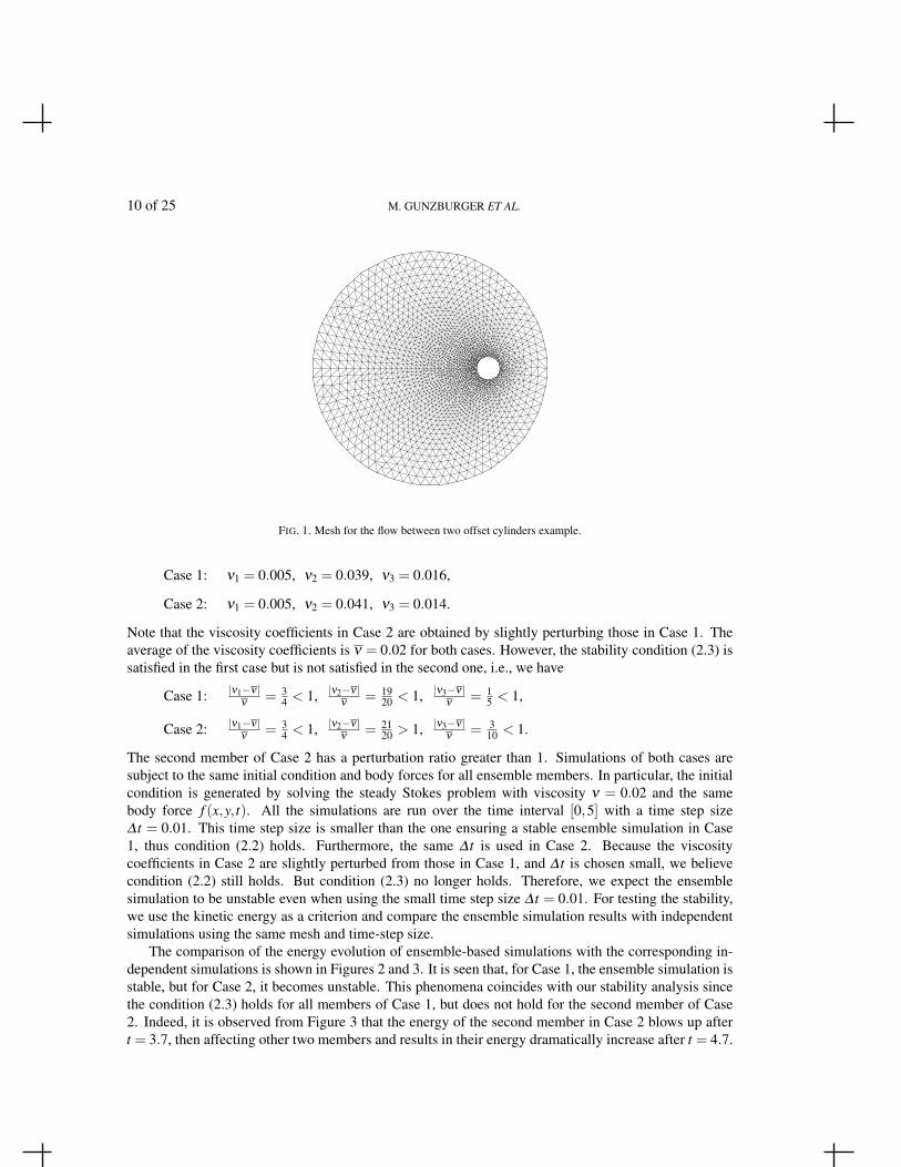
)>with no-slip boundary conditions imposed on both circles. The flow between the two circles showsinteresting structures interacting with the inner circle. A Von Karman vortex street is formed behindthe inner circle and then re-interacts with that circle and with itself, generating complex flow patterns.We consider multiple numerical simulations of the flow with different viscosity coefficients using theensemble-based algorithm (2.1). For spatial discretization, we apply the Taylor-Hood element pair on atriangular mesh that is generated by Delaunay triangulation with 80 mesh points on the outer circle and60 mesh points on the inner circle and with refinement near the inner circle, resulting in 18,638 degreesof freedom; see Figure 1.

In order to illustrate the stability analysis, we select two different sets of viscosity coefficients for:


FIG. 1. Mesh for the flow between two offset cylinders example.

Case 1: ν1 = 0.005, ν2 = 0.039, ν3 = 0.016,

Case 2: ν1 = 0.005, ν2 = 0.041, ν3 = 0.014.

Note that the viscosity coefficients in Case 2 are obtained by slightly perturbing those in Case 1. Theaverage of the viscosity coefficients is ν = 0.02 for both cases. However, the stability condition (2.3) issatisfied in the first case but is not satisfied in the second one, i.e., we have

Case 1: |ν1−ν |ν

= 34 < 1, |ν2−ν |

ν= 19

20 < 1, |ν3−ν |ν

= 15 < 1,

Case 2: |ν1−ν |ν

= 34 < 1, |ν2−ν |

ν= 21

20 > 1, |ν3−ν |ν

= 310 < 1.

The second member of Case 2 has a perturbation ratio greater than 1. Simulations of both cases aresubject to the same initial condition and body forces for all ensemble members. In particular, the initialcondition is generated by solving the steady Stokes problem with viscosity ν = 0.02 and the samebody force f (x,y, t). All the simulations are run over the time interval [0,5] with a time step size∆ t = 0.01. This time step size is smaller than the one ensuring a stable ensemble simulation in Case1, thus condition (2.2) holds. Furthermore, the same ∆ t is used in Case 2. Because the viscositycoefficients in Case 2 are slightly perturbed from those in Case 1, and ∆ t is chosen small, we believecondition (2.2) still holds. But condition (2.3) no longer holds. Therefore, we expect the ensemblesimulation to be unstable even when using the small time step size ∆ t = 0.01. For testing the stability,we use the kinetic energy as a criterion and compare the ensemble simulation results with independentsimulations using the same mesh and time-step size.

The comparison of the energy evolution of ensemble-based simulations with the corresponding in-dependent simulations is shown in Figures 2 and 3. It is seen that, for Case 1, the ensemble simulation isstable, but for Case 2, it becomes unstable. This phenomena coincides with our stability analysis sincethe condition (2.3) holds for all members of Case 1, but does not hold for the second member of Case2. Indeed, it is observed from Figure 3 that the energy of the second member in Case 2 blows up aftert = 3.7, then affecting other two members and results in their energy dramatically increase after t = 4.7.


0 0.5 1 1.5 2 2.5 3 3.5 4 4.5 50

20

40

60

80

100

Time

En

erg

y

ν1=0.005, Ind.

ν1=0.005, Ens.

ν2=0.039, Ind.

ν2=0.039, Ens.

ν3=0.016, Ind.

ν3=0.016, Ens.

FIG. 2. For the flow between two offset cylinders, Case 1, the energy evolution of the ensemble (Ens.) and independent simulations(Ind.).

0 0.5 1 1.5 2 2.5 3 3.5 4 4.5 50

20

40

60

80

100

Time

En

erg

y

ν1=0.005, Ind.

ν1=0.005, Ens.

ν2=0.041, Ind.

ν2=0.041, Ens.

ν3=0.014, Ind.

ν3=0.014, Ens.

FIG. 3. For the flow between two offset cylinders, Case 2, the energy evolution of the ensemble (Ens.) and independent simulations(Ind.).

Next, we use this test example to illustrate the necessity of ensemble simulations. Indeed, theensemble calculation is in great need when flow problems are under parameter uncertainty. This isbecause even though one could obtain a “best estimate” of the parameter that is close enough to the trueparameter value, the corresponding individual solution may vary significantly from the true solutiondue to the nonlinearity of the problems. However, the ensemble mean of the model problems at severalselected parameter samples, which are drawn from a probability distribution (usually experimentallydetermined), tends to smooth out possible errors and gives better forecast than the single run using the“best estimate” parameter value. Here, we consider a simple computational setting in which the trueviscosity ν = 0.01. Due to the errors in measurements, the “best estimate” of the viscosity is 0.00995.


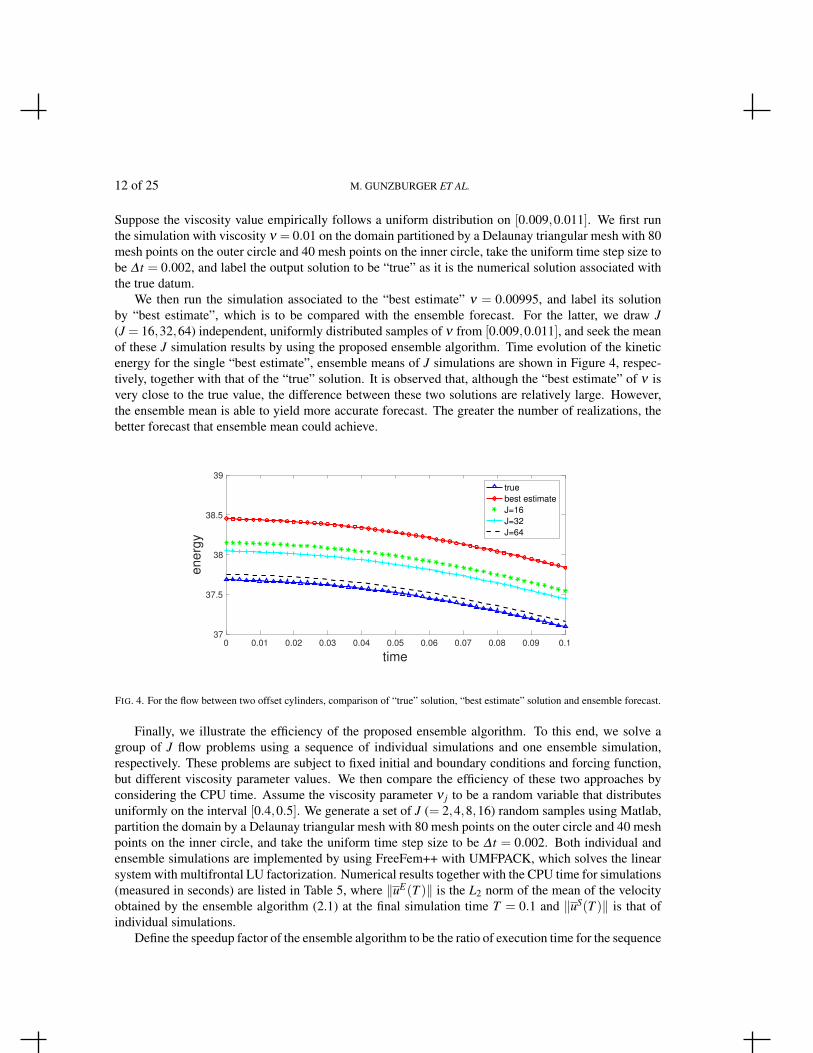
Suppose the viscosity value empirically follows a uniform distribution on [0.009,0.011]. We first runthe simulation with viscosity ν = 0.01 on the domain partitioned by a Delaunay triangular mesh with 80mesh points on the outer circle and 40 mesh points on the inner circle, take the uniform time step size tobe ∆ t = 0.002, and label the output solution to be “true” as it is the numerical solution associated withthe true datum.

We then run the simulation associated to the “best estimate” ν = 0.00995, and label its solutionby “best estimate”, which is to be compared with the ensemble forecast. For the latter, we draw J(J = 16,32,64) independent, uniformly distributed samples of ν from [0.009,0.011], and seek the meanof these J simulation results by using the proposed ensemble algorithm. Time evolution of the kineticenergy for the single “best estimate”, ensemble means of J simulations are shown in Figure 4, respec-tively, together with that of the “true” solution. It is observed that, although the “best estimate” of ν isvery close to the true value, the difference between these two solutions are relatively large. However,the ensemble mean is able to yield more accurate forecast. The greater the number of realizations, thebetter forecast that ensemble mean could achieve.

0 0.01 0.02 0.03 0.04 0.05 0.06 0.07 0.08 0.09 0.1

time

37

37.5

38

38.5

39

energ

y

true

best estimate

J=16

J=32

J=64

FIG. 4. For the flow between two offset cylinders, comparison of “true” solution, “best estimate” solution and ensemble forecast.

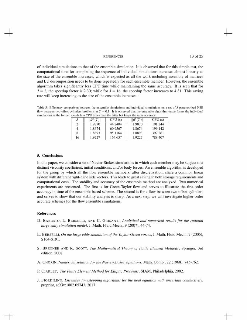
Finally, we illustrate the efficiency of the proposed ensemble algorithm. To this end, we solve agroup of J flow problems using a sequence of individual simulations and one ensemble simulation,respectively. These problems are subject to fixed initial and boundary conditions and forcing function,but different viscosity parameter values. We then compare the efficiency of these two approaches byconsidering the CPU time. Assume the viscosity parameter ν j to be a random variable that distributesuniformly on the interval [0.4,0.5]. We generate a set of J (= 2,4,8,16) random samples using Matlab,partition the domain by a Delaunay triangular mesh with 80 mesh points on the outer circle and 40 meshpoints on the inner circle, and take the uniform time step size to be ∆ t = 0.002. Both individual andensemble simulations are implemented by using FreeFem++ with UMFPACK, which solves the linearsystem with multifrontal LU factorization. Numerical results together with the CPU time for simulations(measured in seconds) are listed in Table 5, where ‖uE(T )‖ is the L2 norm of the mean of the velocityobtained by the ensemble algorithm (2.1) at the final simulation time T = 0.1 and ‖uS(T )‖ is that ofindividual simulations.

Define the speedup factor of the ensemble algorithm to be the ratio of execution time for the sequence

REFERENCES 13 of 25

of individual simulations to that of the ensemble simulation. It is observed that for this simple test, thecomputational time for completing the sequence of individual simulations increases almost linearly asthe size of the ensemble increases, which is expected as all the work including assembly of matricesand LU decomposition needs to be done repeatedly for each ensemble member. However, the ensemblealgorithm takes significantly less CPU time while maintaining the same accuracy. It is seen that forJ = 2, the speedup factor is 2.30; while for J = 16, the speedup factor increases to 4.81. This savingrate will keep increasing as the size of the ensemble increases.

Table 5. Efficiency comparison between the ensemble simulations and individual simulations on a set of J parametrized NSEflow between two offset cylinders problems at T = 0.1. It is observed that the ensemble algorithm outperforms the individualsimulations as the former spends less CPU times than the latter but keeps the same accuracy.

J ‖uE(T )‖ CPU (s) ‖uS(T )‖ CPU (s)2 1.9870 44.2404 1.9870 101.2444 1.8674 60.9567 1.8674 199.1428 1.8893 95.1164 1.8893 397.26116 1.9227 164.637 1.9227 788.407

5. Conclusions

In this paper, we consider a set of Navier-Stokes simulations in which each member may be subject to adistinct viscosity coefficient, initial conditions, and/or body forces. An ensemble algorithm is developedfor the group by which all the flow ensemble members, after discretization, share a common linearsystem with different right-hand side vectors. This leads to great saving in both storage requirements andcomputational costs. The stability and accuracy of the ensemble method are analyzed. Two numericalexperiments are presented. The first is for Green-Taylor flow and serves to illustrate the first-orderaccuracy in time of the ensemble-based scheme. The second is for a flow between two offset cylindersand serves to show that our stability analysis is sharp. As a next step, we will investigate higher-orderaccurate schemes for the flow ensemble simulations.

References

D. BARBATO, L. BERSELLI, AND C. GRISANTI, Analytical and numerical results for the rationallarge eddy simulation model, J. Math. Fluid Mech., 9 (2007), 44-74.

L. BERSELLI, On the large eddy simulation of the Taylor-Green vortex, J. Math. Fluid Mech., 7 (2005),S164-S191.

S. BRENNER AND R. SCOTT, The Mathematical Theory of Finite Element Methods, Springer, 3rdedition, 2008.

A. CHORIN, Numerical solution for the Navier-Stokes equations, Math. Comp., 22 (1968), 745-762.

P. CIARLET, The Finite Element Method for Elliptic Problems, SIAM, Philadelphia, 2002.

J. FIORDILINO, Ensemble timestepping algorithms for the heat equation with uncertain conductivity,preprint, arXiv:1802.05743, 2017.

14 of 25 REFERENCES

J. FIORDILINO, A Second Order Ensemble Timestepping Algorithm for Natural Convection, preprint,arXiv:1708.00488, 2017.

V. GIRAULT AND P.-A. RAVIART, Finite Element Approximation of the Navier-Stokes Equations, Lec-ture Notes in Mathematics, Vol. 749, Springer, Berlin, 1979.

V. GIRAULT AND P.-A. RAVIART, Finite Element Methods for Navier-Stokes Equations - Theory andAlgorithms, Springer, Berlin, 1986.

M. GUNZBURGER, Finite Element Methods for Viscous Incompressible Flows - A Guide to Theory,Practice, and Algorithms, Academic Press, London, 1989.

M. GUNZBURGER, N. JIANG AND M. SCHNEIER, An ensemble-proper orthogonal decompositionmethod for the nonstationary Navier-Stokes equations, SIAM J. Numer. Anal., 55 (2017), 286-304.

M. GUNZBURGER, N. JIANG AND M. SCHNEIER, A higher-order ensemble/proper orthogonal de-composition method for the nonstationary Navier-Stokes Equations, Int. J. Numer. Anal. Model., 15(2018), 608-627.

M. GUNZBURGER, N. JIANG AND Z. WANG, A second-order time-stepping scheme for simulatingensembles of parameterized flow problems, to appear, 2017, Comput. Meth. Appl. Math.

M. GUTKNECHT, Block Krylov space methods for linear systems with multiple right-hand sides: anintroduction, in Modern Mathematical Models, Methods and Algorithms for Real World Systems,Abul Hasan Siddiqi, Iain S. Duff, and Ole Christensen, eds., New Delhi, 2007, Anamaya Publishers,pp. 420-447.

N. JIANG AND H. TRAN, Analysis of a stabilized CNLF method with fast slow wave splittings for flowproblems, Comput. Meth. Appl. Math., 15 (2015), 307-330.

N. JIANG, A higher order ensemble simulation algorithm for fluid flows, J. Sci. Comput., 64 (2015),264-288.

N. JIANG, A second-order ensemble method based on a blended backward differentiation formulatimestepping scheme for time-dependent Navier-Stokes equations, Numer. Meth. Partial. Diff. Eqs.,33 (2017), 34-61.

N. JIANG AND W. LAYTON, An algorithm for fast calculation of flow ensembles, Int. J. Uncertain.Quantif., 4 (2014), 273-301.

N. JIANG AND W. LAYTON, Numerical analysis of two ensemble eddy viscosity numerical regulariza-tions of fluid motion, Numer. Meth. Partial. Diff. Eqs., 31 (2015), 630-651.

N. JIANG, S. KAYA, AND W. LAYTON, Analysis of model variance for ensemble based turbulencemodeling, Comput. Meth. Appl. Math., 15 (2015), 173-188.

V. JOHN AND W. LAYTON, Analysis of numerical errors in large eddy simulation, SIAM J. Numer.Anal., 40 (2002), 995-1020.

W. LAYTON, Introduction to the Numerical Analysis of Incompressible Viscous Flows, Society forIndustrial and Applied Mathematics (SIAM), Philadelphia, 2008.

REFERENCES 15 of 25

Y. LUO AND Z. WANG, An ensemble algorithm for numerical solutions to deterministic and randomparabolic PDEs, SIAM J. Numer. Anal., to appear, 2018.

Y. LUO AND Z. WANG, A Multilevel Monte Carlo Ensemble Scheme for Solving Random ParabolicPDEs, preprint, arXiv:1802.05743, 2018.

M. MOHEBUJJAMAN AND L. REBHOLZ, An efficient algorithm for computation of MHD flow ensem-bles, Comput. Meth. Appl. Math., 17(2017), 121-138.

M. PARKS, K. M. SOODHALTER AND D. B. SZYLD, A block Recycled GMRES method with investi-gations into aspects of solver performance, arXiv preprint arXiv:1604.01713.

D. TAFTI, Comparison of some upwind-biased high-order formulations with a second order central-difference scheme for time integration of the incompressible Navier-Stokes equations, Comput. &Fluids, 25 (1996), 647-665.

A. TAKHIROV, M. NEDA AND J. WATERS, Time relaxation algorithm for flow ensembles, Numer.Meth. Partial. Diff. Eqs., 32 (2016), 757-777.

V. THOMEE, Galerkin finite element methods for parabolic problems, Springer-Verlag Berlin Heidel-berg, 1997.

16 of 25

AppendicesA. Proof of Theorem 2.1

Setting vh = un+1j,h and qh = pn+1

j,h in (2.1) and then adding two equations, we obtain

12‖un+1

j,h ‖2− 1

2‖un

j,h‖2 +12‖un+1

j,h −unj,h‖2 +∆ tb∗(un

j,h−unh,u

nj,h,u

n+1j,h )

+∆ t‖ν12 ∇un+1

j,h ‖2 = ∆ t( f n+1

j ,un+1j,h )−∆ t

((ν j−ν)∇un

j,h,∇un+1j,h

).

Note that ν > νmin > 0. We apply Young’s inequality to the terms on the RHS and have, for ∀α,β > 0,

12‖un+1

j,h ‖2− 1

2‖un

j,h‖2 +12‖un+1

j,h −unj,h‖2 +νmin∆ t‖∇un+1

j,h ‖2 +∆ tb∗(un

j,h−unh,u

nj,h,u

n+1j,h −un

j,h) (A.1)

6ανmin∆ t

8‖∇un+1

j,h ‖2 +

2∆ tανmin

‖ f n+1j ‖2

−1 +βνmin∆ t

4‖∇un+1

j,h ‖2 +‖ν j−ν‖2

∞∆ tβνmin

‖∇unj,h‖2.

Both βνmin∆ t4 ‖∇un+1

j,h ‖2 and ‖ν j−ν‖2∞∆ t

βνmin‖∇un

j,h‖2 on the RHS of (A.1) need to be absorbed into νmin∆ t‖∇un+1j,h ‖

2

on the LHS. To this end, we minimize βνmin∆ t4 +

‖ν j−ν‖2∞∆ tβνmin

by selecting β =2‖ν j−ν‖∞

νminso that (A.1) be-

comes

12‖un+1

j,h ‖2− 1

2‖un

j,h‖2 +12‖un+1

j,h −unj,h‖2 +νmin∆ t‖∇un+1

j,h ‖2 +∆ tb∗(un

j,h−unh,u

nj,h,u

n+1j,h −un

j,h)

6ανmin∆ t

8‖∇un+1

j,h ‖2 +

2∆ tανmin

‖ f n+1j ‖2

−1 +‖ν j−ν‖∞∆ t

2‖∇un+1

j,h ‖2 +‖ν j−ν‖∞∆ t

2‖∇un

j,h‖2.

(A.2)Next, we bound the trilinear term using the inequality (1.9) and the inverse inequality (1.7), obtaining

−∆ tb∗(unj,h−un

h,unj,h,u

n+1j,h −un

j,h)6C∆ t‖∇(unj,h−un

h)‖‖∇unj,h‖[‖∇(un+1

j,h −unj,h)‖‖un+1

j,h −unj,h‖]1/2

6C∆ t‖∇(unj,h−un

h)‖‖∇unj,h‖Ch−

12 ‖un+1

j,h −unj,h‖.

Using Young’s inequality again gives

−∆ tb∗(unj,h−un

h,unj,h,u

n+1j,h −un

j,h)6C∆ t2

h‖∇(un

j,h−unh)‖2‖∇un

j,h‖2 +14‖un+1

j,h −unj,h‖2 . (A.3)

Substituting (A.3) into (A.2) and combining like terms, we have

12‖un+1

j,h ‖2− 1

2‖un

j,h‖2 +14‖un+1

j,h −unj,h‖2 +νmin∆ t

(1− α

4−‖ν j−ν‖∞

2νmin

)‖∇un+1

j,h ‖2 +

α

8νmin∆ t‖∇un+1

j,h ‖2

62∆ t

ανmin‖ f n+1

j ‖2−1 +C

∆ t2

h‖∇(un

j,h−unh)‖2‖∇un

j,h‖2 +‖ν j−ν‖∞∆ t

2‖∇un

j,h‖2.

17 of 25

For any 0 < σ < 1,

12‖un+1

j,h ‖2− 1

2‖un

j,h‖2 +14‖un+1

j,h −unj,h‖2 +

α


j,h ‖2

+νmin∆ t(

1− α

4−‖ν j−ν‖∞

2νmin

)(‖∇un+1

j,h ‖2−‖∇un

j,h‖2)

+νmin∆ t[(1−σ)

(1− α

4−‖ν j−ν‖∞

2νmin

)− C∆ t

νminh‖∇(un

j,h−unh)‖2

]‖∇un

j,h‖2

+νmin∆ t[

σ

(1− α

4−‖ν j−ν‖∞

2νmin

)−‖ν j−ν‖∞

2νmin

]‖∇un

j,h‖2 62∆ t

ανmin‖ f n+1

j ‖2−1 .

(A.4)

Select α = 4− 2(σ+1)σ

√µ . Since α is supposed to be greater than 0, we have

σ >

√µ

2−√µ∈ (0,1). (A.5)

Now taking σ =√

µ+ε

2−√µ, where ε ∈ (0,2−2

√µ) , (A.4) becomes

12‖un+1

j,h ‖2− 1

2‖un

j,h‖2 +14‖un+1

j,h −unj,h‖2 +

α


j,h ‖2

+νmin∆ t(

1− α

4−‖ν j−ν‖∞

2νmin

)(‖∇un+1

j,h ‖2−‖∇un

j,h‖2)

+νmin∆ t[(

(1−σ)σ +1

2σ

√µ− (1−σ)

‖ν j−ν‖∞

2νmin

)− C∆ t

νminh‖∇(un

j,h−unh)‖2

]‖∇un

j,h‖2

+νmin∆ t[

σ +12√

µ− (1+σ)‖ν j−ν‖∞

2νmin

]‖∇un

j,h‖2 62∆ t

ανmin‖ f n+1

j ‖2−1 .

(A.6)

Stability follows if the following conditions hold:

(1−σ)σ +1

2σ

√µ− (1−σ)

12‖ν j−ν‖∞

νmin− C∆ t

νminh‖∇(un

j,h−unh)‖2 > 0, (A.7)

σ +12√

µ− (1+σ)‖ν j−ν‖∞

2νmin> 0. (A.8)

Using assumption (2.3), we have

σ +12√

µ− (1+σ)‖ν j−ν‖∞

2νmin=

2+ ε

2−√µ

(√µ

2−‖ν j−ν‖∞

2νmin

)> 0

so that (A.7) holds. Together with assumption (2.2), we then have

(1−σ)σ +1

2σ

√µ− (1−σ)

12‖ν j−ν‖∞

νmin− C∆ t

νminh‖∇(un

j,h−unh)‖2

> (1−σ)σ +1

2σ

√µ− (1−σ)

12√

µ− C∆ tνminh

‖∇(unj,h−un

h)‖2

=(2−2

√µ− ε)

√µ

2(√

µ + ε)−

(2−2√

µ− ε)√

µ

2(√

µ + ε)= 0,

18 of 25

so (A.8) holds. Therefore, assuming that (2.2) and (2.3) hold, (A.6) reduces to

12‖un+1

j,h ‖2− 1

2‖un

j,h‖2 +14‖un+1

j,h −unj,h‖2 +

ε(2−√µ)

4(√


j,h ‖2

+νmin∆ t(√

µ

22+ ε√

µ + ε−‖ν j−ν‖∞

2νmin

)(‖∇un+1

j,h ‖2−‖∇un

j,h‖2)6


j ‖2−1 .

(A.9)

Summing up (A.9) from n = 0 to n = N−1 results in

12‖uN

j,h‖2 +14

N−1

∑n=0‖un+1

j,h −unj,h‖2 +

N−1

∑n=0

ε(2−√µ)

4(√


j,h ‖2

+νmin∆ t(√

µ

22+ ε√

µ + ε−‖ν j−ν‖∞

2νmin

)‖∇uN

j,h‖2

6N−1

∑n=0


j ‖2−1 +

12‖u0


µ

22+ ε√

µ + ε−‖ν j−ν‖∞

2νmin

)‖∇u0

j,h‖2 .

(A.10)

This completes the proof of stability.

B. Proof of Theorem 3.1

The weak solution of the NSE u j satisfies

(un+1j −un

j

∆ t,vh

)+b∗(un+1

j ,un+1j ,vh)+(ν j∇un+1

j ,∇vh)− (pn+1j ,∇ · vh)

= ( f n+1j ,vh)+ Intp(un+1

j ;vh) , ∀vh ∈Vh,

(B.1)

where Intp(un+1j ;vh) =

(un+1

j −unj

∆ t −u j,t(tn+1),vh

).

Leten

j = unj −un

j,h = (unj −Rhun

j)+(Rhunj −un

j,h) = ηnj +ξ

nj,h,

where Rhunj ∈ Vh is the Ritz projection of un

j onto Vh defined by(

ν ∇(unj −Rhun

j),∇vh

)= 0. The

associated Ritz projection error satisfies (see, e.g., in Thomee (1997))

‖Rhunj −un

j‖+h‖∇(Rhunj −un

j)‖6Chk+1‖unj‖k+1. (B.2)

Subtracting (3.1) from (B.1) gives

(ξn+1j,h −ξ n

j,h

∆ t,vh

)+(ν∇ξ

n+1j,h ,∇vh)+((ν j−ν)∇(un+1

j −unj),∇vh)+((ν j−ν)∇ξ

nj,h,∇vh)

+b∗(un+1j ,un+1

j ,vh)−b∗(unh,u

n+1j,h ,vh)−b∗(un

j,h−unh,u

nj,h,vh)− (pn+1

j ,∇ · vh)

=−

(η

n+1j −ηn

j

∆ t,vh

)− (ν∇η

n+1j ,∇vh)− ((ν j−ν)∇η

nj ,∇vh)+ Intp(un+1

j ;vh).

19 of 25

Setting vh = ξn+1j,h ∈Vh and rearranging the nonlinear terms, we have

1∆ t

(12‖ξ n+1

j,h ‖2− 1

2‖ξ n

j,h‖2 +12‖ξ n+1

j,h −ξnj,h‖2

)+‖ν

12 ∇ξ

n+1j,h ‖

2

=−((ν j−ν)∇(un+1j −un

j),∇ξn+1j,h )− ((ν j−ν)∇ξ

nj,h,∇ξ

n+1j,h )− ((ν j−ν)∇η

nj ,∇ξ

n+1j,h )

−b∗(unj,h−un

h,un+1j,h −un

j,h,ξn+1j,h )−b∗(un+1

j ,un+1j ,ξ n+1

j,h )+b∗(unj,h,u

n+1j,h ,ξ n+1

j,h )

+(pn+1j ,∇ ·ξ n+1

j,h )−

(η

n+1j −ηn

j

∆ t,ξ n+1

j,h

)+ Intp(un+1

j ;ξn+1j,h ).

(B.3)

We first bound the viscous terms on the RHS of (B.3):

−((ν j−ν)∇(un+1j −un

j),∇ξn+1j,h )6 ‖ν j−ν‖∞‖∇(un+1

j −unj)‖‖∇ξ

n+1j,h ‖

61

4C0

‖ν j−ν‖2∞

νmin‖∇(un+1

j −unj)‖2 +C0νmin‖∇ξ

n+1j,h ‖

2

6∆ t4C0

‖ν j−ν‖2∞

νmin

(∫ tn+1

tn‖∇u j,t‖2 dt

)+C0νmin‖∇ξ

n+1j,h ‖

2;

(B.4)

−((ν j−ν)∇ηnj ,∇ξ

n+1j,h )6 ‖ν j−ν‖∞‖∇η

nj ‖‖∇ξ

n+1j,h ‖

61

4C0

‖ν j−ν‖2∞

νmin‖∇η

nj ‖2 +C0νmin‖∇ξ

n+1j,h ‖

2;(B.5)

−(ν j−ν)(∇ξnj,h,∇ξ

n+1j,h )6 ‖ν j−ν‖∞‖∇ξ

nj,h‖‖∇ξ

n+1j,h ‖

61

4C1

‖ν j−ν‖2∞

νmin‖∇ξ

nj,h‖2 +C1νmin‖∇ξ

n+1j,h ‖

2

6‖ν j−ν‖∞

2‖∇ξ

nj,h‖2 +

‖ν j−ν‖∞

2‖∇ξ

n+1j,h ‖

2,

(B.6)

in which we note that both terms on the RHS of (B.6) need to be hidden in the LHS of the error equation,thus C1 =

‖ν j−ν‖∞2νmin

is selected to minimize the summation.Next we analyze the nonlinear terms on the RHS of (B.3) one by one. For the first nonlinear term,

we have−b∗(un

j,h−unh,u

n+1j,h −un

j,h,ξn+1j,h )

=−b∗(unj,h−un

h,en+1j − en

j ,ξn+1j,h )+b∗(un

j,h−unh,u

n+1j −un

j ,ξn+1j,h )

=−b∗(unj,h−un

h,ηn+1j ,ξ n+1

j,h )+b∗(unj,h−un

h,ηnj ,ξ

n+1j,h )

+b∗(unj,h−un

h,ξnj ,ξ

n+1j,h )+b∗(un

j,h−unh,u

n+1j −un

j ,ξn+1j,h ) .

(B.7)

Using inequality (1.8) and Young’s inequality, we have the estimates

−b∗(unj,h−un

h,ηn+1j ,ξ n+1

j,h )6C‖∇(unj,h−un

h)‖‖∇ηn+1j ‖‖∇ξ

n+1j,h ‖

6C2

4C0ν−1min‖∇(un

j,h−unh)‖2‖∇η

n+1j ‖2 +C0νmin‖∇ξ

n+1j,h ‖

2,(B.8)

20 of 25

and−b∗(un

j,h−unh,η

nj ,ξ

n+1j,h )6C‖∇(un

j,h−unh)‖‖∇η

nj ‖‖∇ξ

n+1j,h ‖

6C2




n+1j,h ‖

2.(B.9)

Because b∗(·, ·, ·) is skew-symmetric, we have

b∗(unj,h−un

h,ξnj,h,ξ

n+1j,h ) = b∗(un

j,h−unh,ξ

nj,h−ξ

n+1j,h ,ξ n+1

j,h )

= b∗(unj,h−un

h,ξn+1j,h ,ξ n+1

j,h −ξnj,h) .

Then, by inequality (1.8), we obtain

b∗(unj,h−un

h,ξnj,h,ξ

n+1j,h )6 ‖∇(un

j,h−unh)‖‖∇ξ

nj,h‖‖∇(ξ n+1

j,h −ξnj,h)‖1/2‖ξ n+1

j,h −ξnj,h‖1/2

6C‖∇(unj,h−un

h)‖‖∇ξnj,h‖h−1/2‖ξ n+1

j,h −ξnj,h‖

61

4∆ t‖ξ n+1

j,h −ξnj,h‖2 +

[C

∆ th‖∇(un

j,h−unh)‖2

]‖∇ξ

nj,h‖2.

(B.10)

For the last term of (B.7), we have

b∗(unj,h−un

h,un+1j −un

j ,ξn+1j,h )6C‖∇(un

j,h−unh)‖‖∇(un+1

j −unj)‖‖∇ξ

n+1j,h ‖

6C2


j,h−unh)‖2‖∇(un+1


n+1j,h ‖

2 (B.11)

6C2

4C0∆ tν−1

min‖∇(unj,h−un

h)‖2

(∫ tn+1


)+C0νmin‖∇ξ

n+1j,h ‖

2.

Next, we bound the last two nonlinear terms on the RHS of (B.3) as follows:

−b∗(un+1j ,un+1

j ,ξ n+1j,h )+b∗(un

j,h,un+1j,h ,ξ n+1

j,h )

=−b∗(enj ,u

n+1j ,ξ n+1

j,h )−b∗(unj,h,e

n+1j ,ξ n+1

j,h )−b∗(un+1j −un

j ,un+1j ,ξ n+1

j,h )

=−b∗(ηnj ,u

n+1j ,ξ n+1

j,h )−b∗(ξ nj,h,u

n+1j ,ξ n+1

j,h )−b∗(unj,h,η

n+1j ,ξ n+1

j,h )−b∗(un+1j −un

j ,un+1j ,ξ n+1

j,h ),

(B.12)where, with the assumption un+1

j ∈ L∞(0,T ;H1(Ω)), we have

−b∗(ηnj ,u

n+1j ,ξ n+1

j,h )6C‖∇ηnj ‖‖∇un+1

j ‖‖∇ξn+1j,h ‖

6C2

4C0ν−1min‖∇η


n+1j,h ‖

2.(B.13)

Using the inequality (1.8), Young’s inequality, and un+1j ∈ L∞(0,T ;H1(Ω)), we get

−b∗(ξ nj,h,u

n+1j ,ξ n+1

j,h )6C‖∇ξnj,h‖1/2‖ξ n

j,h‖1/2‖∇un+1j ‖‖∇ξ

n+1j,h ‖

6C‖∇ξnj,h‖1/2‖ξ n

j,h‖1/2‖∇ξn+1j,h ‖

6C( 1

4α‖∇ξ

nj,h‖‖ξ n

j,h‖+α‖∇ξn+1j,h ‖

2)

(B.14)

21 of 25

6C[ 1

4α

(δ

2‖∇ξ

nj,h‖2 +

12δ‖ξ n

j,h‖2)+α‖∇ξn+1j,h ‖

2]

6C0νmin‖∇ξnj,h‖2 +

C4

64C30ν

3min‖ξ n

j,h‖2 +C0νmin‖∇ξn+1j,h ‖

2 ,

where we set α = C0νminC and δ =

8C20 ν

2min

C2 . By Young’s inequality, (1.8), and the result (A.10) from thestability analysis, i.e., ‖un

j,h‖2 6C, we also have

b∗(unj,h,η

n+1j ,ξ n+1

j,h )6C‖∇unj,h‖1/2‖un

j,h‖1/2‖∇ηn+1j ‖‖∇ξ

n+1j,h ‖

6C2

4C0ν−1min‖∇un

j,h‖‖∇ηn+1j ‖2 +C0νmin‖∇ξ

n+1j,h ‖

2,(B.15)

and

b∗(un+1j −un

j ,un+1j ,ξ n+1

j,h )6C‖∇(un+1j −un

j)‖‖∇un+1j ‖‖∇ξ

n+1j,h ‖

6C2

4C0ν−1min‖∇(un+1


n+1j,h ‖

2

=C2

4C0ν−1min∆ t2

∥∥∥∥∥∇un+1j −∇un

j

∆ t

∥∥∥∥∥2

+C0νmin‖∇ξn+1j,h ‖

2 (B.16)

=C2

4C0ν−1min∆ t2

∫Ω

(1

∆ t

∫ tn+1

tn∇u j,t dt

)2

dΩ +C0νmin‖∇ξn+1j,h ‖

2

6C2

4C0ν−1min∆ t

∫ tn+1

tn‖∇u j,t‖2 dt +C0νmin‖∇ξ

n+1j,h ‖

2.

For the pressure term in (B.3), because ξn+1j,h ∈Vh, we have, for any qn+1

j,h ∈ Qh,

(pn+1j ,∇ ·ξ n+1

j,h ) = (pn+1j −qn+1

j,h ,∇ ·ξ n+1j,h )

6√

d ‖pn+1j −qn+1

j,h ‖‖∇ξn+1j,h ‖ (B.17)

61

4dC0ν−1min‖pn+1

j −qn+1j,h ‖

2 +C0 νmin‖∇ξn+1j,h ‖

2 .

The other terms are bounded as(ηn+1j −ηn

j

∆ t,ξ n+1

j,h

)6C

∥∥∥ηn+1j −ηn

j

∆ t

∥∥∥‖∇ξn+1j,h ‖

6C2

4C0ν−1min

∥∥∥∥∥ηn+1j −ηn

j

∆ t

∥∥∥∥∥2


2 (B.18)

6C2

4C0ν−1min

∥∥∥∥∥ 1∆ t

∫ tn+1

tnη j,t dt

∥∥∥∥∥2


2

6C2

4C0ν−1min∆ t−1

∫ tn+1

tn‖η j,t‖2 dt +C0νmin‖∇ξ

n+1j,h ‖

2,

22 of 25

and

Intp(un+1j ;ξ

n+1j,h ) =

(un+1

j −unj

∆ t−u j,t(tn+1),ξ n+1

j,h

)

6C

∥∥∥∥∥un+1j −un

j

∆ t−u j,t(tn+1)

∥∥∥∥∥‖∇ξn+1j,h ‖

6C2

4C0ν−1min

∥∥∥∥∥un+1j −un

j

∆ t−u j,t(tn+1)

∥∥∥∥∥2


2

6C2

4C0ν−1min∆ t

∫ tn+1

tn‖u j,tt‖2 dt +C0νmin‖∇ξ

n+1j,h ‖

2. (B.19)

Combining (B.4)-(B.19), we have

1∆ t

(12||ξ n+1

j,h ||2− 1

2||ξ n

j,h||2 +14‖ξ n+1

j,h −ξnj,h‖2

)+C0νmin‖∇ξ

n+1j,h ‖

2

+νmin

(1−14C0−

‖ν j−ν‖∞

2νmin

)(‖∇ξ

n+1j,h ‖

2−‖∇ξnj,h‖2

)+νmin

[(1−σ)

(1−14C0−

‖ν j−ν‖∞

2νmin

)− C∆ t

νminh‖∇(un

j,h−unh)‖2

]‖∇ξ

nj,h‖2

+νmin

[σ

(1−14C0−

‖ν j−ν‖∞

2νmin

)−‖ν j−ν‖∞

2νmin

]‖∇ξ

nj,h‖2

6C[

1ν

3min‖ξ n

j,h‖2 +∆ t‖ν j−ν‖2

∞

νmin

∫ tn+1

tn‖∇u j,t‖2 dt (B.20)

+‖ν j−ν‖2

∞

νmin‖∇η

nj ‖2 +ν

−1min‖∇(un


n+1j ‖2

+ν−1min‖∇(un


nj ‖2 +ν

−1min∆ t‖∇(un

j,h−unh)‖2

∫ tn+1


+ν−1min‖∇η

nj ‖2 +ν

−1min‖∇un

j,h‖‖∇ηn+1j ‖2 +ν

−1min∆ t

∫ tn+1


+ν−1min‖pn+1

j −qn+1j,h ‖

2 +ν−1min∆ t−1

∫ tn+1

tn‖η j,t‖2 dt +ν

−1min∆ t

∫ tn+1

tn‖u j,tt‖2dt.

]Note that the generic constant C independent of ∆ t is used on the RHS. It, however, depends on thegeometry and mesh due to the use of inverse inequality in (B.10).

Similar to the stability analysis, we take C0 =114 (1−

σ+12σ

√µ) = 1

14ε√

µ+ε(1−

√µ

2 ) with σ =√

µ+ε

2−√µ.

Then, (B.20) becomes

1∆ t

(12||ξ n+1

j,h ||2− 1

2||ξ n

j,h||2 +14‖ξ n+1

j,h −ξnj,h‖2

)+

114

ε√

µ + ε

(1−√

µ

2

)νmin‖∇ξ

n+1j,h ‖

2

+νmin

[√µ

2(2+ ε)√

µ + ε−‖ν j−ν‖∞

2νmin

](‖∇ξ

n+1j,h ‖

2−‖∇ξnj,h‖2

)

23 of 25

+νmin

[2−2

√µ− ε

2−√µ

(√µ

22+ ε√

µ + ε−‖ν j−ν‖∞

2νmin

)− C∆ t

νminh‖∇(un

j,h−unh)‖2

]‖∇ξ

nj,h‖2

+νmin

[√µ + ε

2−√µ

(√µ

22+ ε√

µ + ε−‖ν j−ν‖∞

2νmin

)−‖ν j−ν‖∞

2νmin

]‖∇ξ

nj,h‖2

6C[

1ν

3min‖ξ n

j,h‖2 +∆ t‖ν j−ν‖2

∞

νmin

∫ tn+1

tn‖∇u j,t‖2 dt +νmin‖∇η

n+1j ‖2 (B.21)

+‖ν j−ν‖2

∞

νmin‖∇η

nj ‖2 +ν

−1min‖∇(un


n+1j ‖2

+ν−1min‖∇(un


nj ‖2 +ν


j,h−unh)‖2

∫ tn+1


+ν−1min‖∇η

nj ‖2 +ν

−1min‖∇un

j,h‖‖∇ηn+1j ‖2 +ν

−1min∆ t

∫ tn+1


+ν−1min‖pn+1

j −qn+1j,h ‖

2 +ν−1min∆ t−1

∫ tn+1


−1min∆ t

∫ tn+1

tn‖u j,tt‖2dt .

]By the convergence condition (3.3), we have

√µ

2(2+ ε)√

µ + ε−‖ν j−ν‖∞

2νmin>√

µ

2(2+ ε)√

µ + ε−√

µ

2> 0,

and√

µ + ε

2−√µ

(√µ

22+ ε√

µ + ε−‖ν j−ν‖∞

2νmin

)−‖ν j−ν‖∞

2νmin

>√

µ + ε

2−√µ

(√µ

22+ ε√

µ + ε−√

µ

2

)−√

µ

2

>√

µ + ε

2−√µ

(√µ

22−√µ√

µ + ε

)−√

µ

2>√

µ

2−√

µ

2= 0

and by the convergence conditions (3.2) and (3.3), we have

2−2√

µ− ε

2−√µ

(√µ

22+ ε√

µ + ε−‖ν j−ν‖∞

2νmin

)− C∆ t

νminh‖∇(un

j,h−unh)‖2

>2−2

√µ− ε

2−√µ

(√µ

22−√µ√

µ + ε

)−

(2−2√

µ− ε)√

µ

2(√

µ + ε)

>(2−2

√µ− ε)

√µ

2(√

µ + ε)−

(2−2√

µ− ε)√

µ

2(√

µ + ε)> 0.

Summing (B.20) from n = 1 to N−1 and multiplying both sides by ∆ t gives

12‖ξ N

j,h‖2 +14

N−1

∑n=0‖ξ n+1

j,h −ξnj,h‖2 +

114

ε√

µ + ε(1−

√µ

2)νmin∆ t

N−1

∑n=0‖∇ξ

n+1j,h ‖

2

+νmin∆ t[√

µ

2(2+ ε)√

µ + ε−‖ν j−ν‖∞

2νmin

]‖∇ξ

Nj,h‖2

24 of 25

612‖ξ 0

j,h‖2 +νmin∆ t[√

µ

2(2+ ε)√

µ + ε−‖ν j−ν‖∞

2νmin

]‖∇ξ

0j,h‖2 +

C∆ tν

3min

N−1

∑n=0‖ξ n

j,h‖2

+C∆ tN−1

∑n=0

[∆ t‖ν j−ν‖2

∞

νmin

∫ tn+1

tn‖∇u j,t‖2 dt +νmin‖∇η

n+1j ‖2

+‖ν j−ν‖2

∞

νmin‖∇η

nj ‖2 +ν

−1min‖∇(un


n+1j ‖2

+ν−1min‖∇(un


nj ‖2 +ν


j,h−unh)‖2

∫ tn+1


+ν−1min‖∇η

nj ‖2 +ν

−1min∆ t

∫ tn+1

tn‖∇u j,t‖2 dt +ν

−1min‖∇η

n+1j ‖2‖∇un

j,h‖

+ν−1min‖pn+1

j −qn+1j,h ‖

2 +ν−1min∆ t−1

∫ tn+1


−1min∆ t

∫ tn+1

tn‖u j,tt‖2 dt

].

Using the Ritz projection error (B.2) and the result (2.4) from the stability analysis, i.e., ∆ t ∑N−1n=0 ‖∇un

j,h‖26C, we have

Cν−1min∆ t

N−1

∑n=0‖∇η

n+1j ‖2‖∇un

j,h‖6Cν−1minh2k

∆ tN−1

∑n=0‖un+1

j ‖2k+1‖2‖∇un

j,h‖ (B.22)

6Cν−1minh2k

(∆ t

N−1

∑n=0‖un+1

j ‖4k+1 +∆ t

N−1

∑n=0‖∇un

j,h‖2

)(B.23)

6Cν−1minh2k∣∣∣∣∣∣u j

∣∣∣∣∣∣44,k+1 +Cν

−1minh2k.

By applying again the Ritz projection error (B.2) and the interpolation error (1.6), we have

12‖ξ N


µ

2(2+ ε)√

µ + ε−‖ν j−νmin‖∞

2νmin

]‖∇ξ

Nj,h‖2 +

N−1

∑n=0

14‖ξ n+1

j,h −ξnj,h‖2

+1

15ε

√µ + ε

(1−√

µ

2)νmin∆ t

N−1

∑n=0‖∇ξ

n+1j,h ‖

2

612‖ξ 0


µ

2(2+ ε)√

µ + ε−‖ν j−ν‖∞

2νmin

]‖∇ξ

0j,h‖2 +

C∆ tν

3min

N−1

∑n=0‖ξ n

j,h‖2 (B.24)

+C∆ t2 ‖ν j−ν‖2∞

νmin‖∇u j,t‖2

2,0 +Cνminh2k∣∣∣∣∣∣u j∣∣∣∣∣∣2

2,k+1 +C‖ν j−ν‖2

∞


∣∣∣∣∣∣22,k+1

+Ch2k+1∆ t−1∣∣∣∣∣∣u j

∣∣∣∣∣∣22,k+1 +Ch∆ t‖∇u j,t‖2

2,0 +Cν−1minh2k∣∣∣∣∣∣u j

∣∣∣∣∣∣22,k+1

+Cν−1min∆ t2‖∇u j,t‖2

2,0 +Cν−1minh2k∣∣∣∣∣∣u j

∣∣∣∣∣∣44,k+1 +Cν

−1minh2k

+Cν−1minh2s+2∣∣∣∣∣∣p j

∣∣∣∣∣∣22,s+1 +Cν

−1minh2k+2‖u j,t‖2

2,k+1 +Cν−1min∆ t2‖u j,tt‖2

2,0.

The next step is the application of the discrete Gronwall inequality (see Girault et al. (1979, p. 176)):

12‖ξ N


µ

2(2+ ε)√

µ + ε−‖ν j−ν‖∞

2νmin

)‖∇ξ

Nj,h‖2 +

N−1

∑n=0

14‖ξ n+1

j,h −ξnj,h‖2

25 of 25

+114

ε√

µ + ε(1−

√µ

2)νmin∆ t

N−1

∑n=0‖∇ξ

n+1j,h ‖

2 (B.25)

6 eCT

ν3min

12‖ξ 0


µ

2(2+ ε)√

µ + ε−‖ν j−ν‖∞

2νmin

]‖∇ξ

0j,h‖2

+C[∆ t2 ‖ν j−ν‖2

∞

νmin

∣∣∣∣∣∣∇u j,t∣∣∣∣∣∣2

2,0 +νminh2k∣∣∣∣∣∣u j∣∣∣∣∣∣2

2,k+1 +‖ν j−ν‖2

∞


∣∣∣∣∣∣22,k+1

+h2k+1∆ t−1∣∣∣∣∣∣u j

∣∣∣∣∣∣22,k+1 +Ch∆ t

∣∣∣∣∣∣∇u j,t∣∣∣∣∣∣2

2,0 +ν−1minh2k∣∣∣∣∣∣u j

∣∣∣∣∣∣22,k+1

+ν−1min∆ t2∣∣∣∣∣∣∇u j,t

∣∣∣∣∣∣22,0 +ν

−1minh2k∣∣∣∣∣∣u j

∣∣∣∣∣∣44,k+1 +ν

−1minh2k

+ν−1minh2s+2∣∣∣∣∣∣p j

∣∣∣∣∣∣22,s+1 +ν

−1minh2k+2∣∣∣∣∣∣u j,t

∣∣∣∣∣∣22,k+1 +ν

−1min∆ t2∣∣∣∣∣∣u j,tt

∣∣∣∣∣∣22,0

].

Recall that enj = ηn

j +ξ nj,h. Using the triangle inequality on the error equation to split the error terms

into terms of ηnj and ξ n

j,h gives

12‖eN

j ‖2 +1

14ε

√µ + ε

(1−√

µ

2

)νmin∆ t

N−1

∑n=0‖∇en+1

j ‖2

612‖ξ N

j,h‖2 +114

ε√

µ + ε

(1−√

µ

2

)νmin∆ t

N−1

∑n=0‖∇ξ

n+1j,h ‖

2

+12‖ηN

j ‖2 +1

14ε

√µ + ε

(1−√

µ

2

)νmin∆ t

N−1

∑n=0‖∇η

n+1j ‖2,

and12‖ξ 0

j,h‖2 +

[√µ

2(2+ ε)√

µ + ε−‖ν j−ν‖∞

2νmin

]νmin∆ t‖∇ξ

0j,h‖2

612‖e0

j‖2 +

[√µ

2(2+ ε)√

µ + ε−

ν j−ν‖∞

2νmin

]νmin∆ t‖∇e0

j‖2

+12‖η0

j ‖2 +

[√µ

2(2+ ε)√

µ + ε−

ν j−ν‖∞

2νmin

]νmin∆ t‖∇η

0j ‖2 .

Applying inequality (B.25), using the previous bounds for ηnj terms, and absorbing constants into a new

constant C, completes the proof of Theorem 3.1.

an efﬁcient algorithm for simulating ensembles of

Documents