materials

Article

An Efficient and Adaptable Path Planning Algorithmfor Automated Fiber Placement Based on Meshingand Multi Guidelines

Hong Xiao 1,*, Wei Han 1, Wenbin Tang 1,2 and Yugang Duan 1

1 State Key Lab for Manufacturing Systems Engineering, Xi’an Jiaotong University, Xi’an 710049, China;jx18hanwei@stu.xjtu.edu.cn (W.H.); tangwb@xpu.edu.cn (W.T.); ygduan@xjtu.edu.cn (Y.D.)

2 School of Mechanical and Electrical Engineering, Xi’an Polytechnic University, Xi’an 710048, China* Correspondence: xiaohongjxr@xjtu.edu.cn

Received: 11 August 2020; Accepted: 18 September 2020; Published: 22 September 2020

Abstract: Path planning algorithms for automated fiber placement are used to determine the directionsof the fiber paths and the start and end positions on the mold surfaces. The quality of the fiber pathsdetermines largely the efficiency and quality of the automated fiber placement process. The presentedwork investigated an efficient path planning algorithm based on surface meshing. In addition,an update method of the datum direction vector via a guide-line update strategy was proposed tomake the path planning algorithm applicable for complex surfaces. Finally, accuracy analysis wasperformed on the proposed algorithm and it can be adopted as the reference for the triangulationparameter selection for the path planning algorithm.

Keywords: fiber-reinforced polymers; automated fiber placement; path planning

1. Introduction

Fiber-reinforced polymers (FRPs), especially carbon fiber reinforced polymers (CFRPs), are widelyused in the aerospace and automobile industry as well as other fields because of their highspecific strength, high specific modulus, excellent corrosion- and fatigue-resistance, and outstandingdesignability [1]. Automated fiber placement combines special manufacturing equipment withcomputerized numerical control (CNC) systems, which enables good forming quality, strongadaptability, and high efficiency. As an advanced composite manufacturing technology of largeand complex components, automated fiber placement has become one of the most advanced andcutting-edge technologies for composite forming [2]. Path planning algorithms for automated fiberplacement are used to specify the direction of a fiber path and determine the start and end positions ofthe fiber on the mold surface. The quality of the fiber path plays a crucial role for the efficiency andquality of the fiber placement process.

At present, the typical fiber path planning algorithms include the geodesic method and themeshing method based on parametric surfaces. The path planning algorithm of geodesic method basedon parametric surfaces includes analytical and numerical methods [3]. The fiber path, which is obtainedvia the numerical solution of geodesics, is more aligned with practical engineering requirements.Lewis et al. [4] proposed a path planning method based on natural path, which is also widely usedfor path planning of tape laying. Shirinzadeh et al. [5–7] put forward the method of intersectinglines and surfaces to build the initial path, which improves the adaptability of the path to the surfacecurvature. However, there are certain disadvantages with the numerical solution of geodesics, e.g.,the difficulty of finding the solution and the low efficiency associated with the calculation [8,9].The meshing method, which uses the polygonal meshes to describe the complex parametric surfaces,

Materials 2020, 13, 4209; doi:10.3390/ma13184209 www.mdpi.com/journal/materials

Materials 2020, 13, 4209 2 of 18

can reduce computational complexity. The deviation of the fiber path correlates with the accuracy ofthe meshing [10,11]. Shinno et al. [12] proposed an iterative geodesic algorithm for a quadrilateralmesh surface to obtain the fiber path. Li et al. [13] proposed a path planning algorithm which usedthe mesh information contained in the STL file. However, there is a lack of quantitative analysis ofthe efficiency of the fiber path planning algorithm based on meshed surfaces. Also, no deviationanalysis was performed for the generated fiber paths. Meanwhile, for complex components (surfaces),the design of angle reference direction datum is too simple, which leads to the poor applicability of thealgorithm, fiber wrinkles, and eventually, affects the quality and mechanical properties of the fabricatedFRP components. In this paper, a path planning algorithm for automated fiber placement based onmeshing and multi guide-lines was proposed. Both the efficiency and accuracy of the algorithm wereanalyzed. The outline of the proposed algorithm is shown in Figure 1.

Materials 2020, 13, x FOR PEER REVIEW 2 of 19

with the accuracy of the meshing [10,11]. Shinno et al. [12] proposed an iterative geodesic algorithm for a quadrilateral mesh surface to obtain the fiber path. Li et al. [13] proposed a path planning algorithm which used the mesh information contained in the STL file. However, there is a lack of quantitative analysis of the efficiency of the fiber path planning algorithm based on meshed surfaces. Also, no deviation analysis was performed for the generated fiber paths. Meanwhile, for complex components (surfaces), the design of angle reference direction datum is too simple, which leads to the poor applicability of the algorithm, fiber wrinkles, and eventually, affects the quality and mechanical properties of the fabricated FRP components. In this paper, a path planning algorithm for automated fiber placement based on meshing and multi guide-lines was proposed. Both the efficiency and accuracy of the algorithm were analyzed. The outline of the proposed algorithm is shown in Figure 1.

Figure 1. The outline of the proposed algorithm for automated fiber placement.

2. Efficiency Analysis and Topology Reconstruction

2.1. Efficiency Analysis of the Proposed Algorithm

A traditional path planning algorithm based on the geodesic method of parametric surface generates fiber paths by solving the direction of each point on the surface. It mainly uses the two geometric numerical solution operations, i.e., the intersection between a surface and a plane and the parallel offset of a curve. Essentially, the parallel offset of a curve is realized by the intersection of the surface at the sampling points and the corresponding offset direction planes.

Commercial CAD / CAM softwares generally use NURBS (Non-Uniform Rational B-Splines) for modelling, and the NURBS surface is represented by the following parameter equations: = ( , )= ( , )= ( , ) (1)

s( , ) = ∑ ∑ , , , ( ) , ( )∑ ∑ , , ( ) , ( ) (2)

where Ω is the domain of s, , is the control point, , is the weight, , ( ) is the basis function of the pth-order B-spline in u direction, and , ( ) is the basis function of the qth-order B-spline in v direction.

Let the plane be represented by an implicit surface equation: ℎ( , , ) = 0 (3)

where Ω is the domain of h. Combining Equation (1) with Equation (3) yields the intersection of plane h and surface s in

domain Ω = Ω ∩ Ω . The parameters u and v of the intersection line satisfy the equation for the intersection line [14]： ℎ ( , ), ( , ), ( , ) = ( , ) = 0 (4)

Intersection line l is a plane curve in the plane of parameter fields for u and v. If the surface s is the p × q-th order, the intersection line l is the p × q-th order. Because of the low efficiency of high-

Figure 1. The outline of the proposed algorithm for automated fiber placement.

2. Efficiency Analysis and Topology Reconstruction

2.1. Efficiency Analysis of the Proposed Algorithm

A traditional path planning algorithm based on the geodesic method of parametric surfacegenerates fiber paths by solving the direction of each point on the surface. It mainly uses the twogeometric numerical solution operations, i.e., the intersection between a surface and a plane and theparallel offset of a curve. Essentially, the parallel offset of a curve is realized by the intersection of thesurface at the sampling points and the corresponding offset direction planes.

Commercial CAD/CAM softwares generally use NURBS (Non-Uniform Rational B-Splines) formodelling, and the NURBS surface is represented by the following parameter equations:

x = sx(u, v)y = sy(u, v)z = sz(u, v)

(1)

s(u, v) =

∑Cui=0

∑Cvj=0 Wi, jPi, jNi,p(u)N j,q(v)∑Cu

i=0∑Cv

j=0 Wi, jNi,p(u)N j,q(v)(2)

where Ωs is the domain of s, Pi, j is the control point, Wi, j is the weight, Ni,p(u) is the basis functionof the pth-order B-spline in u direction, and N j,q(v) is the basis function of the qth-order B-spline inv direction.

Let the plane be represented by an implicit surface equation:

h(x, y, z) = 0 (3)

where Ωh is the domain of h.Combining Equation (1) with Equation (3) yields the intersection of plane h and surface s in

domain Ω = Ωh ∩ Ωs. The parameters u and v of the intersection line satisfy the equation for theintersection line [14]:

h(sx(u, v), sy(u, v), sz(u, v)

)= l(u, v) = 0 (4)

Materials 2020, 13, 4209 3 of 18

Intersection line l is a plane curve in the plane of parameter fields for u and v. If the surfaces is the p × q-th order, the intersection line l is the p × q-th order. Because of the low efficiency ofhigh-precision floating-point calculations, the frequent and high-precision solution of the intersectionequation l consumes a lot of resources. This decreases both efficiency and stability of the numericalalgorithms for the intersection between surfaces and planes. In the path planning algorithm based onthe parametric surfaces, the intersection between surfaces and planes needs to be solved frequently.This decreases the efficiency of the path calculation, and for complex surfaces, the equation order is toohigh to be solved, which leads to the failure of path planning.

For triangular mesh surfaces, the surface is approximately a plane within the mesh cell [15].The intersection between the surface and the plane can be converted into an intersection betweenplanes, and the straight line in the plane is the result of the intersection.

The intersection line equation of a triangular patch Ai(x, y, z) = 0 and the plane h is:

l′(x, y, z) = 0 (5)x = x0 + mty = y0 + ntz = z0 + pt

(6)

The intersection line l′ is the first order equation about t, and the solution complexity decreasessignificantly. Since the triangulation algorithm will generate discrete grid planes of different sizeswith different model complexity, the algorithm will not increase the order and complexity of equationsolution during path generation due to the increase of model complexity. Therefore, the fiber pathplanning algorithm based on triangular mesh surface can obtain stable numerical solution quicklyand efficiently.

2.2. Triangulation Algorithm for Parametric Surface

In the triangulation algorithm used in this paper, the edge and inner surfaces of the cell surfaceare approximated by straight line segments. Hence, the surface is discretized into area strips, and it isfurther divided into plane triangles. The triangulation results for the surface are generally given asstrips of triangles. A strip of triangles is a list of points, such that any three consecutive points define atriangle. A parametric surface can be approximated by a series of triangle strips.

Due to the approximation process of replacing a curved surface with plane surfaces, the discreteerror occurs in the triangulation process for parametric surface. This error is mainly reflected in thedistance between the meshed plane surfaces and the original parametric surface. Two triangulationparameters are used to constrain the approximation error: (a) Dl2s: The maximum distance fromthe straight-line segment of the discrete triangular area to the original parametric surface. (b) Lseg:The maximum length of the straight-line segment in the discrete triangular area.

2.3. Sub-surface Boundary Splicing and Surface Topology Reconstruction

NURBS curves and surfaces, which are widely used in CAD/CAM software, have exactmathematical expressions, strong expression ability, good quality, and are easy to control. However,for complex surfaces, NURBS surfaces need to be split, spliced and trimmed. A complex surface isusually composed of multiple cellular surfaces. To reconstruct the topology of the whole complexsurface, in addition to the mesh reconstruction of the cellular parameter surfaces, boundary splicingbetween cellular patches should be performed to obtain the global geometric topology.

2.3.1. Topology Reconstruction Algorithm for the Triangular Mesh of a Cellular Patch

As mentioned above, a cellular surface can be split into feature sampling points. To restore thesurface information, it is necessary to obtain the segmentation results and establish the data structurefor the triangular meshes by the vertex aggregation algorithm for triangulation (Algorithm 1).

Materials 2020, 13, 4209 4 of 18

Algorithm 1: Vertex aggregation algorithm for triangulation

Input: All vertex sets after the triangulation of a cellular parametric surface.Output: Face ID List, Edge ID List and Point ID List for this cellular parametric surface.1: Loop all strip, fans and triangles:2: According to the right-hand rule, the vertices in the current discrete cell are stored to form the Point IDList of the current cell parameter surface.3: Loop all points in the Point ID List4: Every three points in the point table form a triangle patch to summarize the Face ID list and store theindexes of the three points of the current triangle patch.5: Point ID List update, add triangle patch ID index.6: Build the edge ID list, update the two-point indexes of the edge, update the Point ID list to add the edgeindex, update the Face ID list to add the included edge index.7: Calculate the normal vector of the current triangular patch according to the right-hand rule, and update it inthe Face ID list.

Through the above process, the local Point ID list, Edge ID list and Face ID list are established,which reconstruct the topology information for the current NURBS cellular surface.

2.3.2. Algorithm for Subsurface-Boundary Splicing

Because the mesh discretization results for each cellular parameter surface are independent ofeach other, and two adjacent cellular surfaces share the same edge, there are duplicate vertices for theadjacent cellular surfaces. It is necessary to remove the duplicate vertices. The subsurface-boundarysplicing algorithm includes removing duplicate vertices and updating the global index of the verticesin all the cellular surfaces.

The brute force algorithm, which traverses the whole Point ID List for the duplicate verticeswith the same coordinates with a given vertex and hence delete the duplicate ones, is the moststraightforward method. Suppose that the surface is made up of k quadrilateral cellular NURBSsurfaces with similar area and all the NURBS surfaces are smooth. Following the triangulation, it wasassumed that the triangulation results are all given as strips of triangles to obtain a uniform triangularnetwork. If the number of vertices on the boundary is a and b, the number of vertices on the cellularsurface is a × b, and the number of all vertices is N = k × a × b. The time complexity of the brute forcealgorithm is O(N2).

However, all the duplicate vertices are located on the boundary line because they are formed bytwo adjacent cellular surfaces sharing a common edge. For the vertices on the boundary line, they arein a semi-closed state and not surrounded by all triangles. On the other hand, the vertices inside thesurfaces are in a fully-closed state, surrounded by several triangles (Figure 2). When the vertex is inthe fully-closed state, the number of adjacent patches is equal to the number of edges, while in thesemi-closed state, the number of patches is not equal to the number of edges. Therefore, all trianglevertices can be divided into two types: boundary semi-closed vertices and internal fully-closed vertices.Thanks to this feature, the boundary vertex set can be filtered out. Then, duplicate vertices canbe removed from the boundary vertex set, and Point ID list, Face ID list and Edge ID list can beupdated simultaneously.

Materials 2020, 13, 4209 5 of 18

Materials 2020, 13, x FOR PEER REVIEW 5 of 19

Algorithm 2: De-duplication algorithm based on vertex closure checking Input：Point ID list before de-duplication. Output：Point ID list after de-duplication. 1: Find semi-closed state vertices 2: Loop all points in all Point ID List: 3: if point->edgenum != point->facenum 4: save this point to duplicate Point ID List; 5: Loop all point1 in duplicate Point ID List: 6: Loop all point2 in duplicate Point ID List: 7: if point1.distanceto (point2) < eps 8: delete point2 in Point ID List; 9: refresh Face ID List & Edge ID List;

The time complexity of the algorithm is O (k × (a + b)2), which is far less than O (N2) of the brute force algorithm, and the efficiency of the algorithm is greatly improved.

Figure 2. Internal fully-closed points and boundary semi-closed points in cell parametric surfaces.

At the end of the above process, both sub-surface boundary splicing and surface topological relation reconstruction are completed. This enables fast search of adjacent triangles and efficient path calculation. The topological information of the discrete mesh surfaces is contained in the Point ID list, Face ID list and Edge ID list. The forms and requirements of the three data structure list are shown in Table 1 [13].

Table 1. The forms and requirements of the three data structure lists.

Class Contents Features

Vertex

int vIndex; double p [3];

int EdgeIndexList [cur edge index]; int FaceIndexList [cur face index];

Given the index number of a vertex, one can quickly find the global index of the triangle

patch and the global index for the edge, where the current vertex belongs.

Edge int eIndex;

int VertexIndexList [2]; int FaceIndexList [2];

Given the number of a side, one can quickly find the global index of the face, where the

current edge belongs and the global indices of the two vertices at the current edge.

Face

int fIndex; doubla n [3];

int VertexIndexList [3]; int EdgeIndexList [3];

Given the number of a triangle patch, one can quickly find the global index and the global index of the three edges of the three vertices

on the triangle patch.

Figure 2. Internal fully-closed points and boundary semi-closed points in cell parametric surfaces.

De-duplication algorithm based on the vertex closure checking was described in Algorithm 2.

Algorithm 2: De-duplication algorithm based on vertex closure checking

Input: Point ID list before de-duplication.Output: Point ID list after de-duplication.1: Find semi-closed state vertices2: Loop all points in all Point ID List:3: if point->edgenum != point->facenum4: save this point to duplicate Point ID List;5: Loop all point1 in duplicate Point ID List:6: Loop all point2 in duplicate Point ID List:7: if point1.distanceto (point2) < eps8: delete point2 in Point ID List;9: refresh Face ID List & Edge ID List;

The time complexity of the algorithm is O (k × (a + b)2), which is far less than O (N2) of the bruteforce algorithm, and the efficiency of the algorithm is greatly improved.

At the end of the above process, both sub-surface boundary splicing and surface topologicalrelation reconstruction are completed. This enables fast search of adjacent triangles and efficient pathcalculation. The topological information of the discrete mesh surfaces is contained in the Point ID list,Face ID list and Edge ID list. The forms and requirements of the three data structure list are shown inTable 1 [13].

Table 1. The forms and requirements of the three data structure lists.

Class Contents Features

Vertex

int vIndex;double p [3];

int EdgeIndexList [cur edge index];int FaceIndexList [cur face index];

Given the index number of a vertex, one can quickly find theglobal index of the triangle patch and the global index for

the edge, where the current vertex belongs.

Edgeint eIndex;

int VertexIndexList [2];int FaceIndexList [2];

Given the number of a side, one can quickly find the globalindex of the face, where the current edge belongs and the

global indices of the two vertices at the current edge.

Faceint fIndex;

doubla n [3];int VertexIndexList [3];int EdgeIndexList [3];

Given the number of a triangle patch, one can quickly findthe global index and the global index of the three edges of

the three vertices on the triangle patch.

3. Main Path Planning Algorithm Based on Guidelines on Triangular Mesh Surfaces

The path planning process needs to generate the main motion paths of the head of the automatedfiber placement equipment and the corresponding fiber paths which are offset by the main motion

Materials 2020, 13, 4209 6 of 18

paths. The fiber path generation is relatively simple and this paper focuses on the main path planningalgorithm. The guidelines are extracted from the CAD model of the mold of the to-be-fabricatedFRP component to reflect the skeleton and unique appearance of the component. According to theguide-lines, the direction vector of the main path can be calculated and adjusted adaptively, so thatthe main path and the corresponding fiber paths can comply with the shape of the component.It is beneficial to improve the mechanical performances of the FRP component while satisfying theconstraints of the minimum steering radius of the fiber materials, even distribution of the cuttingpoints, etc.

3.1. Main Motion Path Generation Algorithm

According to the fiber placement process, three geometric parameters (initial starting point P0,guide line L, parametric surface Π) as well as the ply angle θ should be provided as input to the mainmotion path generation algorithm, which outputs the main motion path li. Basically, the algorithmneeds to calculate the direction vectors and subsequently generate the continuous points on the mainmotion path, as described in Algorithms 3 and 4, respectively.

Algorithm 3: The direction vector calculation algorithm for the main motion path.Step 1: Find the projection point P0’ for the initial starting point P0 on the triangle patch A of the

triangular mesh surfaces∑

(triangulation of the parametric surface Π) and obtain the normal vector nof triangle patch A. Then, redefine P0’ as the starting point for the current main motion path.

Step 2: Calculate the tangent vector t’ for the projection point P0” of P0’ on the guide line L,and generate the parallel vector t of t’ at point P0’.

Step 3: Calculate the orthogonal vector k of the normal vector n and the parallel tangent vector t,where k = n × t.

Step 4: Calculate the orthogonal vector m of normal vector n and vector k, where m = k × n.The vector m is the datum direction vector for the current path point, based on the guide-line andcorrected by the curvature feature of the surface, where the path point is located (as shown in Figure 3).

Materials 2020, 13, x FOR PEER REVIEW 6 of 19

3. Main Path Planning Algorithm Based on Guidelines on Triangular Mesh Surfaces

The path planning process needs to generate the main motion paths of the head of the automated fiber placement equipment and the corresponding fiber paths which are offset by the main motion paths. The fiber path generation is relatively simple and this paper focuses on the main path planning algorithm. The guidelines are extracted from the CAD model of the mold of the to-be-fabricated FRP component to reflect the skeleton and unique appearance of the component. According to the guide-lines, the direction vector of the main path can be calculated and adjusted adaptively, so that the main path and the corresponding fiber paths can comply with the shape of the component. It is beneficial to improve the mechanical performances of the FRP component while satisfying the constraints of the minimum steering radius of the fiber materials, even distribution of the cutting points, etc.

3.1. Main Motion Path Generation Algorithm

According to the fiber placement process, three geometric parameters (initial starting point P0, guide line L, parametric surface Π) as well as the ply angle θ should be provided as input to the main motion path generation algorithm, which outputs the main motion path li. Basically, the algorithm needs to calculate the direction vectors and subsequently generate the continuous points on the main motion path, as described in Algorithms 3 and 4, respectively.

Algorithm 3: The direction vector calculation algorithm for the main motion path. Step 1: Find the projection point P0’ for the initial starting point P0 on the triangle patch A of the

triangular mesh surfaces ∑ (triangulation of the parametric surface Π) and obtain the normal vector n of triangle patch A. Then, redefine P0’ as the starting point for the current main motion path.

Step 2: Calculate the tangent vector t’ for the projection point P0’’ of P0’ on the guide line L, and generate the parallel vector t of t’ at point P0’.

Step 3: Calculate the orthogonal vector k of the normal vector n and the parallel tangent vector t, where k = n × t.

Step 4: Calculate the orthogonal vector m of normal vector n and vector k, where m = k × n. The vector m is the datum direction vector for the current path point, based on the guide-line and corrected by the curvature feature of the surface, where the path point is located (as shown in Figure 3).

Step 5: Using normal vector n as the rotation axis, rotate the datum direction vector m for θ degree to obtain the laying direction vector d for the current path point P0’.

= cos −sin 0sin cos 00 0 1 × (7)

Figure 3. Illustration of the direction vector calculation algorithm. Figure 3. Illustration of the direction vector calculation algorithm.

Step 5: Using normal vector n as the rotation axis, rotate the datum direction vector m for θ degreeto obtain the laying direction vector d for the current path point P0’.

d =

cosθ − sinθ 0sinθ cosθ 0

0 0 1

×m (7)

In the current triangle patch A, use point P0′ and vector d to construct a straight line andhence obtain the intersection point P1 of the straight line and the three sides of triangle patch A.

Materials 2020, 13, 4209 7 of 18

The intersection point P1 is the next path point, and all the path points can be obtained after continuousiteration for the main motion path generation.

Algorithm 4: The continuous path point generation algorithm.Step 1: Take the starting point Pi and direction vector di in the current triangle patch Ai, construct

a ray Pa (λ), which is defined as the solution line for the path point. Its parameter equation is:

Pa(λ) = Pi + λ·d (8)

Step 2: The vertices Va and Vb of the triangle patch form a straight line Pb (λ), and the parameterequation is:

Pb(λ) = (1− λ)·Va + λ·Vb (9)

Step 3: Using Pa(λ) = Pb(λ), we can find the unique solution λ:

λ =Va − Pi

d +→

Va−Vb

‖→

Va−Vb‖

(10)

If 0 ≤ λ ≤ 1 is true, this means that the next path point is on the current sideline. If it is not on thecurrent sideline, then take two points to form a straight line for the calculation. Next, take VcVb andVaVc to form a straight line for the calculation. Repeat steps 1, 2, and 3 to get the next path point.

The solution line for the path point may overlap with the three side lines of the triangle in step 3,and the next path point Pi+1 cannot be calculated using the above steps. At this time, the endpoint ofthe edge VmVk(m, k ∈ a, b, c) of the triangle, where the point Pi is located, is used as the next path pointPi+1. The endpoint selection rules are described in Equation (11), where d is the laying direction vector.

Pi+1 =

Vk, d ∗VmVk = 1Vm, otherwise

(11)

Step 4: According to the topological relationship for the triangular mesh surface, obtain theadjacent triangles on the other side of the edge, where Pi+1 is located, and update the patch indexas Ai+1.

Step 5: Update the normal vector ni+1. When the next path point Pi+1 lies on the triangle edge orvertex, use the area weighing method to reduce the deviation.

n =

∑mk=1 Ak·nk∣∣∣∑mk=1 Ak·nk

∣∣∣ (12)

In Equation (12), m is the total number of adjacent triangles to which Pi+1 belongs, and Ak is thearea of the triangles. The area can be determined using Ak = ‖AB×AC‖

2 , where points A, B, C are thethree vertices of a triangle Ak.

Step 6: Update the parallel tangent vector ti+1, and solve the direction vector di+1 of the next pathpoint Pi+1 using Algorithm 3. The projection vector di+1′ of di+1 on patch Ak+1 is the laying-directionvector of point Pi+1.

d′i+1 = di+1 −di+1·n

‖n‖2·n (13)

Step 7: Repeat Step 1 to Step 6 to update and calculate the next path point until reach the triangularmesh surface boundary and no adjacent patch can be found and the partial path on the one singledirection is constructed.

Step 8: Go back to the path initial point P0, take the inverse of the laying-direction vector d0 andrepeat Step 1 to Step 7 until the whole main motion path is completely constructed.

Materials 2020, 13, 4209 8 of 18

The continuous path point generation algorithm is shown in Figure 4. After completing the abovesteps, the main motion path can be derived using the cubic spline interpolation algorithm.Materials 2020, 13, x FOR PEER REVIEW 8 of 19

Figure 4. Continuous path point generation algorithm. (a) Calculation of next point in single triangle patch. (b) Calculation of all points of one path on the triangular mesh surfaces.

3.2. Guide-line Update Algorithm for Complex Surfaces

If the curvature of the surface of certain components changes substantially, the path, which was calculated and planned using a single guide line, cannot meet the requirements for the laying ability in each surface area. This leads to wrinkling of the fiber during the laying process, which degrades the mechanical properties of the final fabricated components. To address this problem, this paper proposed a guide-line algorithm for the update of the tangent vector t and datum direction vector m for the path points according to the surface shape and the distribution of multi guide-lines, as demonstrated in Figure 5 and described in Algorithm 5.

Figure 5. Guide-line update algorithm for complex surfaces: (a) Distribution diagram for multi guide-lines. (b) Polygonal section formed by the projection point of the point on the guide-line. (c) Diagram of tangent vector calculation.

Figure 4. Continuous path point generation algorithm. (a) Calculation of next point in single trianglepatch. (b) Calculation of all points of one path on the triangular mesh surfaces.

3.2. Guide-line Update Algorithm for Complex Surfaces

If the curvature of the surface of certain components changes substantially, the path, which wascalculated and planned using a single guide line, cannot meet the requirements for the laying ability ineach surface area. This leads to wrinkling of the fiber during the laying process, which degrades themechanical properties of the final fabricated components. To address this problem, this paper proposeda guide-line algorithm for the update of the tangent vector t and datum direction vector m for the pathpoints according to the surface shape and the distribution of multi guide-lines, as demonstrated inFigure 5 and described in Algorithm 5.

Materials 2020, 13, x FOR PEER REVIEW 8 of 19

Figure 4. Continuous path point generation algorithm. (a) Calculation of next point in single triangle patch. (b) Calculation of all points of one path on the triangular mesh surfaces.

3.2. Guide-line Update Algorithm for Complex Surfaces

If the curvature of the surface of certain components changes substantially, the path, which was calculated and planned using a single guide line, cannot meet the requirements for the laying ability in each surface area. This leads to wrinkling of the fiber during the laying process, which degrades the mechanical properties of the final fabricated components. To address this problem, this paper proposed a guide-line algorithm for the update of the tangent vector t and datum direction vector m for the path points according to the surface shape and the distribution of multi guide-lines, as demonstrated in Figure 5 and described in Algorithm 5.

Figure 5. Guide-line update algorithm for complex surfaces: (a) Distribution diagram for multi guide-lines. (b) Polygonal section formed by the projection point of the point on the guide-line. (c) Diagram of tangent vector calculation.

Figure 5. Guide-line update algorithm for complex surfaces: (a) Distribution diagram for multiguide-lines. (b) Polygonal section formed by the projection point of the point on the guide-line.(c) Diagram of tangent vector calculation.

Algorithm 5: Guideline update algorithm for complex surfaces.

Materials 2020, 13, 4209 9 of 18

Step 1: Project the current path point Pi on each guide-line Li to obtain projection points A, B, Cand D. Connect the projection points to form a polygonal section plane Ω, the four sides of the polygonon the section plane Ω are a, b, c and d.

Step 2: Project the current path point Pi to the edge of the polygon, and find the projection pointsP1

i , P2i , P3

i and P4i .

Step 3: If the projection point is on the extension line of the edge, the edge is excluded. As shownin Figure 5b, the projection point P4

i is not on the edge d, so the edge d is not considered in thealgorithm below.

Step 4: Calculate the distance from Pi to the projection points on the not excluded edge lines,where dist = ‖PiPx

i ‖.Step 5: Determine the minimum distance dist and its edge x. The two guide-lines La and Lb, at the

end of x, are the guide-lines for the current path point Pi.Step 6: As shown in Figure 5c and Equation (14), calculate the tangent vectors on La and Lb,

respectively. The smooth transition for the path direction vector from La to Lb is realized using thedistance-weighing method:

t =t1·dist1 + t2·dist2

dist1 + dist2(14)

where dist1 and dist2 are the distances of Pi to La and Lb.Update the tangent vector t and calculate the datum direction vector m of Pi in Algorithms 3 and 4.

The path, which is generated by Algorithm 5, is more adaptive to the changing curvature of the surfaceand the scalability is improved. Figure 6 shows the paths generated based on single guideline andmulti-guidelines for a panel and a curved surface models. It can be seen that the fiber direction transitssmoothly between the guide lines and this makes the placed fibers adapt to the shape of the moulds ofthe final parts.

Materials 2020, 13, x FOR PEER REVIEW 9 of 19

Algorithm 5: Guideline update algorithm for complex surfaces. Step 1: Project the current path point Pi on each guide-line Li to obtain projection points A, B, C

and D. Connect the projection points to form a polygonal section plane Ω, the four sides of the polygon on the section plane Ω are a, b, c and d.

Step 2: Project the current path point Pi to the edge of the polygon, and find the projection points , , and .

Step 3: If the projection point is on the extension line of the edge, the edge is excluded. As shown in Figure 5b, the projection point is not on the edge d, so the edge d is not considered in the algorithm below.

Step 4: Calculate the distance from Pi to the projection points on the not excluded edge lines, where = ‖ ‖.

Step 5: Determine the minimum distance dist and its edge x. The two guide-lines La and Lb, at the end of x, are the guide-lines for the current path point Pi.

Step 6: As shown in Figure 5c and Equation (14), calculate the tangent vectors on La and Lb, respectively. The smooth transition for the path direction vector from La to Lb is realized using the distance-weighing method: = ∙ + ∙+ (14)

where dist1 and dist2 are the distances of Pi to La and Lb. Update the tangent vector t and calculate the datum direction vector m of Pi in Algorithms 3 and

4. The path, which is generated by Algorithm 5, is more adaptive to the changing curvature of the surface and the scalability is improved. Figure 6 shows the paths generated based on single guideline and multi-guidelines for a panel and a curved surface models. It can be seen that the fiber direction transits smoothly between the guide lines and this makes the placed fibers adapt to the shape of the moulds of the final parts.

Figure 6. The paths generated based on single guide line and multi-guide lines for a panel (a,b) and a curved surface (c,d) models.

Figure 6. The paths generated based on single guide line and multi-guide lines for a panel (a,b) and acurved surface (c,d) models.

Materials 2020, 13, 4209 10 of 18

4. Accuracy Analysis of the Generated Path Based on Surface Meshing

In the triangulation process in Section 2, Dl2s and Lseg are the main parameters that affect boththe mesh density and the approximation accuracy. When the two parameters are set to larger values,the mesh density is small, the surface approximation accuracy is low, the subsequent path planningprocess data volume is small, and the algorithm efficiency is high. If the two parameter values arecontinuously reduced, on the other hand, the efficiency is lower.

It is generally believed that the path generated using the geodesic method on the parametricsurface is used as the standard path when the planning accuracy and error of the algorithm need tobe verified. The points on the discrete surface of the mesh are used to replace the path points onthe original parametric surface. Furthermore, the normal vector of the path points on the triangularmesh surface can be used to replace the normal vector on the original parametric surface. As a result,a cumulative error can occur during the iteration process of the proposed path planning algorithm,which can cause the angle deviation from the design datum and the distance deviation from the pathgenerated on the original parametric surface.

A complex surface with positive and negative curvature was adopted to conduct accuracy analysisof the proposed path planning algorithm, as shown in Figure 7. The surface consists of 29 independentcellular patches. Each cellular parameter surface represents a NURBS surface, and the order of eachcellular parameter surface in both U and V directions is 6 degrees.

Materials 2020, 13, x FOR PEER REVIEW 10 of 19

4. Accuracy Analysis of the Generated Path Based on Surface Meshing

In the triangulation process in Section 2, Dl2s and Lseg are the main parameters that affect both the mesh density and the approximation accuracy. When the two parameters are set to larger values, the mesh density is small, the surface approximation accuracy is low, the subsequent path planning process data volume is small, and the algorithm efficiency is high. If the two parameter values are continuously reduced, on the other hand, the efficiency is lower.

It is generally believed that the path generated using the geodesic method on the parametric surface is used as the standard path when the planning accuracy and error of the algorithm need to be verified. The points on the discrete surface of the mesh are used to replace the path points on the original parametric surface. Furthermore, the normal vector of the path points on the triangular mesh surface can be used to replace the normal vector on the original parametric surface. As a result, a cumulative error can occur during the iteration process of the proposed path planning algorithm, which can cause the angle deviation from the design datum and the distance deviation from the path generated on the original parametric surface.

A complex surface with positive and negative curvature was adopted to conduct accuracy analysis of the proposed path planning algorithm, as shown in Figure 7. The surface consists of 29 independent cellular patches. Each cellular parameter surface represents a NURBS surface, and the order of each cellular parameter surface in both U and V directions is 6 degrees.

Figure 7. Illustration of the surface for accuracy analysis. (a) Original parametric surface. (b) Triangular mesh surface with Dl2s = 0.2 and Lseg = 100. (c) Surface curvature variation diagram for the path-deviation-error test area.

4.1. Distance Deviation Analysis

The distance deviation of the path generated on the triangular mesh surface can be decomposed into the normal distance deviation and the geodesic distance deviation. In this paper, a uniform orthogonal test was carried out for the appropriate ranges of Dl2s and Lseg. The path was uniformly sampled (with a distance of 5 mm) to evaluate the distance deviation, as shown in Figure 8.

During the triangulation process, both Dl2s and Lseg did not reach 0, which means that the parameter value (without approximation error) could not be determined. Therefore, in the actual application, the Dl2s range was 0.2–1.0 mm, and the Lseg range was 20–200 mm. The experiment was carried out by the (5 ) orthogonal design. The path-generation time, the distance deviation, the normal distance deviation and the geodesic distance deviation were recorded.

Figure 7. Illustration of the surface for accuracy analysis. (a) Original parametric surface. (b) Triangularmesh surface with Dl2s = 0.2 and Lseg = 100. (c) Surface curvature variation diagram for thepath-deviation-error test area.

4.1. Distance Deviation Analysis

The distance deviation of the path generated on the triangular mesh surface can be decomposedinto the normal distance deviation and the geodesic distance deviation. In this paper, a uniformorthogonal test was carried out for the appropriate ranges of Dl2s and Lseg. The path was uniformlysampled (with a distance of 5 mm) to evaluate the distance deviation, as shown in Figure 8.

During the triangulation process, both Dl2s and Lseg did not reach 0, which means that theparameter value (without approximation error) could not be determined. Therefore, in the actualapplication, the Dl2s range was 0.2–1.0 mm, and the Lseg range was 20–200 mm. The experimentwas carried out by the L25

(56

)orthogonal design. The path-generation time, the distance deviation,

the normal distance deviation and the geodesic distance deviation were recorded.The Euclidean distance deviation d from the sample point on the generated path to the standard

reference path was calculated and decomposed into the normal distance deviation dN and the geodesicdistance deviation dT.

Materials 2020, 13, 4209 11 of 18

Materials 2020, 13, x FOR PEER REVIEW 11 of 19

Figure 8. Standard path, verification path generated by the new algorithm, and sample points for Dl2s = 0.4 and Lseg = 100.

The Euclidean distance deviation d from the sample point on the generated path to the standard reference path was calculated and decomposed into the normal distance deviation dN and the geodesic distance deviation dT.

The project vector from the sample point to standard reference path is V, and the normal vector for sample point Pi on the original parametric surface is n. dN and dT can be calculated as follows: = ( , )= × < , >− (15)

According to the (5 ) orthogonal design, 25 sets of experiments were carried out. Four of them, which were Dl2s = 0.2 and Lseg = 65, Dl2s =0.4 and Lseg = 110, Dl2s = 0.6 and Lseg = 155 and Dl2s = 0.8 and Lseg = 200, were selected to analyze the distribution of distance deviation along the generated paths.

The initial path point was located near the 350th sample point. According to Figure 9, the closer the sample point was to the initial point, the smaller was the distance deviation. During path generation, the normal vector for the path points on the triangular mesh surface was used to (approximately) replace the normal vector of the path points on the original parameter surface. Therefore, the direction datum of the path point was deviated, and it caused geodesic distance deviation between the generated path and the standard reference path. It also shows that the geodesic distance deviation dT was the main deviation and it increased as the parameters Dl2s and Lseg increased.

To analyze the relationship between the parameters (i.e., Dl2s and Lseg) and the distance deviation of the generated path and the algorithm efficiency, the mean distance deviation, the normal mean distance deviation, the geodesic mean distance deviation, the maximum distance deviation, the maximum normal distance deviation, the maximum geodesic distance deviation, and the path generation time were calculated. This was done when the generation time started from the beginning of the surface triangulation to the end of the path generation, as shown in Table 2.

Figure 8. Standard path, verification path generated by the new algorithm, and sample points forDl2s = 0.4 and Lseg = 100.

The project vector from the sample point to standard reference path is V, and the normal vectorfor sample point Pi on the original parametric surface is n. dN and dT can be calculated as follows:

d = DistBetween(Pi, P′i

)dN = d× cos< V, n >

dT =√

d2 − d2N

(15)

According to the L25(56

)orthogonal design, 25 sets of experiments were carried out. Four of

them, which were Dl2s = 0.2 and Lseg = 65, Dl2s = 0.4 and Lseg = 110, Dl2s = 0.6 and Lseg = 155 andDl2s = 0.8 and Lseg = 200, were selected to analyze the distribution of distance deviation along thegenerated paths.

The initial path point was located near the 350th sample point. According to Figure 9, the closer thesample point was to the initial point, the smaller was the distance deviation. During path generation,the normal vector for the path points on the triangular mesh surface was used to (approximately)replace the normal vector of the path points on the original parameter surface. Therefore, the directiondatum of the path point was deviated, and it caused geodesic distance deviation between the generatedpath and the standard reference path. It also shows that the geodesic distance deviation dT was themain deviation and it increased as the parameters Dl2s and Lseg increased.

To analyze the relationship between the parameters (i.e., Dl2s and Lseg) and the distance deviation ofthe generated path and the algorithm efficiency, the mean distance deviation, the normal mean distancedeviation, the geodesic mean distance deviation, the maximum distance deviation, the maximumnormal distance deviation, the maximum geodesic distance deviation, and the path generation timewere calculated. This was done when the generation time started from the beginning of the surfacetriangulation to the end of the path generation, as shown in Table 2.

Materials 2020, 13, 4209 12 of 18

Materials 2020, 13, x FOR PEER REVIEW 12 of 19

Figure 9. The distance deviation distribution (N Distance is dN and T Distance is dT.) for different parameters (a) Dl2s = 0.2,Lseg = 65, (b) Dl2s = 0.4,Lseg = 110, (c) Dl2s = 0.6,Lseg = 155 and (d) Dl2s = 0.8, Lseg = 200.

Table 2. Distance deviation and generation time.

Dl2s /mm

Lseg /mm

Mean Distance

Deviation /mm

Normal Mean

Distance Deviation

/mm

Geodesic Mean

Distance Deviation

/mm

Maximum Distance

Deviation /mm

Maximum Normal

Distance Deviation

/mm

Maximum Geodesic Distance

Deviation /mm

Generation Time

/s

0.2 20 0.41072 0.00824 0.40834 0.81222 0.05218 0.81219 5.506 0.2 65 0.45268 0.02694 0.4329 1.29759 0.16468 1.29745 0.549 0.2 110 0.57411 0.02534 0.55406 1.60354 0.16447 1.60342 0.508 0.2 155 0.57298 0.02557 0.55294 1.60354 0.16447 1.60342 0.508 0.2 200 0.57309 0.02547 0.55304 1.60354 0.16447 1.60342 0.505 0.4 20 0.41072 0.00824 0.40834 0.81222 0.05218 0.81219 5.514 0.4 65 0.54446 0.09072 0.47922 2.12237 0.36747 2.12172 0.296 0.4 110 0.78375 0.09412 0.71355 3.00629 0.46252 3.00561 0.214 0.4 155 0.78403 0.09052 0.71476 2.94274 0.46246 2.94204 0.209 0.4 200 0.78403 0.09052 0.71476 2.94274 0.46246 2.94204 0.213 0.6 20 0.41072 0.00824 0.40834 0.81222 0.05218 0.81219 5.495 0.6 65 0.62143 0.1036 0.55255 2.14027 0.55588 2.13962 0.231 0.6 110 0.65292 0.20369 0.4915 1.62566 0.77333 1.62391 0.142 0.6 155 0.86012 0.18893 0.69804 3.09987 0.77349 3.0993 0.13 0.6 200 0.8602 0.18895 0.6985 3.08182 0.77349 3.08124 0.128 0.8 20 0.41072 0.00824 0.40834 0.81222 0.05218 0.81219 5.499 0.8 65 0.62315 0.10188 0.55424 2.19272 0.55588 2.19207 0.213 0.8 110 0.78546 0.20771 0.63916 1.94612 0.84012 1.94459 0.115

Figure 9. The distance deviation distribution (N Distance is dN and T Distance is dT.) for differentparameters (a) Dl2s = 0.2, Lseg = 65, (b) Dl2s = 0.4, Lseg = 110, (c) Dl2s = 0.6, Lseg = 155 and (d) Dl2s = 0.8,Lseg = 200.

Table 2. Distance deviation and generation time.

Dl2s/mm

Lseg/mm

MeanDistanceDeviation

/mm

Normal MeanDistance

Deviation/mm

Geodesic MeanDistance

Deviation/mm

MaximumDistance

Deviation/mm

MaximumNormalDistance

Deviation/mm

MaximumGeodesicDistance

Deviation/mm

GenerationTime

/s

0.2 20 0.41072 0.00824 0.40834 0.81222 0.05218 0.81219 5.5060.2 65 0.45268 0.02694 0.4329 1.29759 0.16468 1.29745 0.5490.2 110 0.57411 0.02534 0.55406 1.60354 0.16447 1.60342 0.5080.2 155 0.57298 0.02557 0.55294 1.60354 0.16447 1.60342 0.5080.2 200 0.57309 0.02547 0.55304 1.60354 0.16447 1.60342 0.5050.4 20 0.41072 0.00824 0.40834 0.81222 0.05218 0.81219 5.5140.4 65 0.54446 0.09072 0.47922 2.12237 0.36747 2.12172 0.2960.4 110 0.78375 0.09412 0.71355 3.00629 0.46252 3.00561 0.2140.4 155 0.78403 0.09052 0.71476 2.94274 0.46246 2.94204 0.2090.4 200 0.78403 0.09052 0.71476 2.94274 0.46246 2.94204 0.2130.6 20 0.41072 0.00824 0.40834 0.81222 0.05218 0.81219 5.4950.6 65 0.62143 0.1036 0.55255 2.14027 0.55588 2.13962 0.2310.6 110 0.65292 0.20369 0.4915 1.62566 0.77333 1.62391 0.1420.6 155 0.86012 0.18893 0.69804 3.09987 0.77349 3.0993 0.130.6 200 0.8602 0.18895 0.6985 3.08182 0.77349 3.08124 0.1280.8 20 0.41072 0.00824 0.40834 0.81222 0.05218 0.81219 5.4990.8 65 0.62315 0.10188 0.55424 2.19272 0.55588 2.19207 0.2130.8 110 0.78546 0.20771 0.63916 1.94612 0.84012 1.94459 0.1150.8 155 1.18547 0.19293 1.03511 3.91933 0.84004 3.91922 0.0980.8 200 1.15638 0.19065 1.00657 3.8031 0.84004 3.80299 0.1031 20 0.41072 0.00824 0.40834 0.81222 0.05218 0.81219 5.4911 65 0.62147 0.10314 0.55262 2.14027 0.55588 2.13962 0.2031 110 0.83477 0.2216 0.68092 2.01082 1.10312 2.00955 0.1051 155 1.33796 0.21533 1.16792 3.97448 1.10346 3.97407 0.0821 200 1.29659 0.20791 1.12927 3.81894 1.10346 3.8185 0.083

The distribution of mean distance deviation are shown in Figure 10, while the maximumdistance deviation are shown in Figure 11, and the generation time are shown in Figure 12.

Materials 2020, 13, 4209 13 of 18

Supplementary Video S1 further demonstrates the high efficiency of the proposed algorithm, which cancomplete the path planning for one layer of a complex surface in just only tens of seconds.

Materials 2020, 13, x FOR PEER REVIEW 13 of 19

0.8 155 1.18547 0.19293 1.03511 3.91933 0.84004 3.91922 0.098 0.8 200 1.15638 0.19065 1.00657 3.8031 0.84004 3.80299 0.103 1 20 0.41072 0.00824 0.40834 0.81222 0.05218 0.81219 5.491 1 65 0.62147 0.10314 0.55262 2.14027 0.55588 2.13962 0.203 1 110 0.83477 0.2216 0.68092 2.01082 1.10312 2.00955 0.105 1 155 1.33796 0.21533 1.16792 3.97448 1.10346 3.97407 0.082 1 200 1.29659 0.20791 1.12927 3.81894 1.10346 3.8185 0.083

The distribution of mean distance deviation are shown in Figure 10, while the maximum distance deviation are shown in Figure 11, and the generation time are shown in Figure 12.

Figure 10. Mean distance deviation and its decomposition.

Figure 11. Maximum distance deviation and its decomposition.

Figure 10. Mean distance deviation and its decomposition.

Materials 2020, 13, x FOR PEER REVIEW 13 of 19

0.8 155 1.18547 0.19293 1.03511 3.91933 0.84004 3.91922 0.098 0.8 200 1.15638 0.19065 1.00657 3.8031 0.84004 3.80299 0.103 1 20 0.41072 0.00824 0.40834 0.81222 0.05218 0.81219 5.491 1 65 0.62147 0.10314 0.55262 2.14027 0.55588 2.13962 0.203 1 110 0.83477 0.2216 0.68092 2.01082 1.10312 2.00955 0.105 1 155 1.33796 0.21533 1.16792 3.97448 1.10346 3.97407 0.082 1 200 1.29659 0.20791 1.12927 3.81894 1.10346 3.8185 0.083

The distribution of mean distance deviation are shown in Figure 10, while the maximum distance deviation are shown in Figure 11, and the generation time are shown in Figure 12.

Figure 10. Mean distance deviation and its decomposition.

Figure 11. Maximum distance deviation and its decomposition. Figure 11. Maximum distance deviation and its decomposition.

According to Figures 10 and 11, for different parameters, the distance deviation mainly consistedof geodesic distance deviation, and the effect of normal distance deviation on the overall distancedeviation is relatively small. Meanwhile, it can be observed that Dl2s and Lseg restricted each other inthe triangulation process. When the two parameters cannot be satisfied simultaneously, the algorithmwill adopt the parameter that makes the mesh more precise. For example, when Lseg is 20 mm,the triangulation algorithm generated the same triangular mesh surfaces for a Dl2s of 0.4 mm, 0.6 mm,0.8 mm and 1.0 mm as for the Dl2s of 0.2 mm.

Table 2 shows that, when Dl2s exceeds 0.8mm and Lseg exceeds 155 mm, the mean distancedeviation surpasses 1mm, and the maximum distance deviation exceeds 2 mm. When Dl2s is between

Materials 2020, 13, 4209 14 of 18

0.2 and 0.6mm, and Lseg is 65 to 155 mm, the average distance deviation remains within 1mm, while themaximum distance deviation is within 2 mm. The generation time of the algorithm is within 0.5 s.

Materials 2020, 13, x FOR PEER REVIEW 14 of 19

Figure 12. The generation times.

According to Figures 10 and 11, for different parameters, the distance deviation mainly consisted of geodesic distance deviation, and the effect of normal distance deviation on the overall distance deviation is relatively small. Meanwhile, it can be observed that Dl2s and Lseg restricted each other in the triangulation process. When the two parameters cannot be satisfied simultaneously, the algorithm will adopt the parameter that makes the mesh more precise. For example, when Lseg is 20 mm, the triangulation algorithm generated the same triangular mesh surfaces for a Dl2s of 0.4 mm, 0.6 mm, 0.8 mm and 1.0 mm as for the Dl2s of 0.2 mm.

Table 2 shows that, when Dl2s exceeds 0.8mm and Lseg exceeds 155 mm, the mean distance deviation surpasses 1mm, and the maximum distance deviation exceeds 2 mm. When Dl2s is between 0.2 and 0.6mm, and Lseg is 65 to 155 mm, the average distance deviation remains within 1mm, while the maximum distance deviation is within 2 mm. The generation time of the algorithm is within 0.5 s.

4.2. Angle Deviation Analysis

To ensure the orthogonal arrangement of fibers in different layers, the angle distribution between different layers is strictly defined. This ensures quasi-isotropic mechanical behavior for the components [3]. To analyze the angle deviation between the generated paths and the design datum, an angle deviation analysis was performed in this section.

The generated path was sampled uniformly with a step of 5 mm. For each sample point, the forward direction of the current path and the design direction datum of the path were calculated using both the guide-line and surface normal vector at the point. Subsequently, the angle deviation was obtained. The forward direction vector at each sample point is the tangent vector of the sample point on the path. The datum direction vector can be calculated using: = ×= × (16)

Figure 12. The generation times.

4.2. Angle Deviation Analysis

To ensure the orthogonal arrangement of fibers in different layers, the angle distributionbetween different layers is strictly defined. This ensures quasi-isotropic mechanical behavior for thecomponents [3]. To analyze the angle deviation between the generated paths and the design datum,an angle deviation analysis was performed in this section.

The generated path was sampled uniformly with a step of 5 mm. For each sample point,the forward direction of the current path and the design direction datum of the path were calculatedusing both the guide-line and surface normal vector at the point. Subsequently, the angle deviationwas obtained. The forward direction vector di at each sample point is the tangent vector of the samplepoint on the path. The datum direction vector d′i can be calculated using:

k′i = n′i × t′id′i = n′i × k′i

(16)

where n′i is the normal vector of the sample point on the surface, and t′i is the tangent of the projectionpoint for the sample point on the guide-line. The angle deviation δi is calculated using:

δi = arcos< di, d′i > (17)

The four sets of experiments selected in Section 4.1 were also adopted here to analyze thedistribution of the angle deviation.

As mentioned above, the initial path point was near the 350th sampling point. According toFigure 13, for different triangulation parameters, the angle deviation does not depend on the distancebetween the sampling point and the initial path point but depend on the curvature of the originalsurface. The larger the curvature of the surface, where the sample points are located on the path,

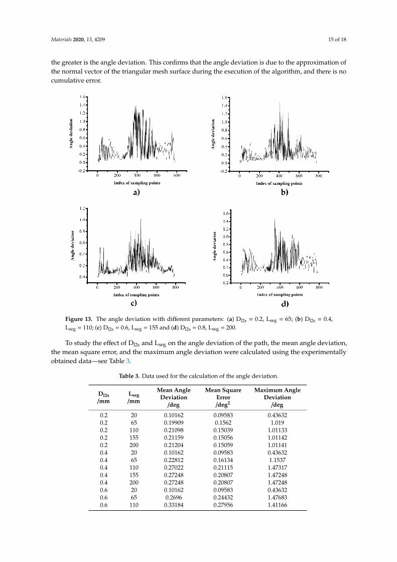
Materials 2020, 13, 4209 15 of 18

the greater is the angle deviation. This confirms that the angle deviation is due to the approximation ofthe normal vector of the triangular mesh surface during the execution of the algorithm, and there is nocumulative error.

Materials 2020, 13, x FOR PEER REVIEW 15 of 19

where is the normal vector of the sample point on the surface, and is the tangent of the projection point for the sample point on the guide-line. The angle deviation is calculated using: = < , > (17)

The four sets of experiments selected in Section 4.1 were also adopted here to analyze the distribution of the angle deviation.

As mentioned above, the initial path point was near the 350th sampling point. According to Figure 13, for different triangulation parameters, the angle deviation does not depend on the distance between the sampling point and the initial path point but depend on the curvature of the original surface. The larger the curvature of the surface, where the sample points are located on the path, the greater is the angle deviation. This confirms that the angle deviation is due to the approximation of the normal vector of the triangular mesh surface during the execution of the algorithm, and there is no cumulative error.

Figure 13. The angle deviation with different parameters: (a) Dl2s = 0.2, Lseg = 65; (b) Dl2s = 0.4, Lseg = 110; (c) Dl2s = 0.6, Lseg = 155 and (d) Dl2s = 0.8, Lseg = 200.

To study the effect of Dl2s and Lseg on the angle deviation of the path, the mean angle deviation, the mean square error, and the maximum angle deviation were calculated using the experimentally obtained data—see Table 3.

Figure 13. The angle deviation with different parameters: (a) Dl2s = 0.2, Lseg = 65; (b) Dl2s = 0.4,Lseg = 110; (c) Dl2s = 0.6, Lseg = 155 and (d) Dl2s = 0.8, Lseg = 200.

To study the effect of Dl2s and Lseg on the angle deviation of the path, the mean angle deviation,the mean square error, and the maximum angle deviation were calculated using the experimentallyobtained data—see Table 3.

Table 3. Data used for the calculation of the angle deviation.

Dl2s/mm

Lseg/mm

Mean AngleDeviation

/deg

Mean SquareError/deg2

Maximum AngleDeviation

/deg

0.2 20 0.10162 0.09583 0.436320.2 65 0.19909 0.1562 1.0190.2 110 0.21098 0.15039 1.011330.2 155 0.21159 0.15056 1.011420.2 200 0.21204 0.15059 1.011410.4 20 0.10162 0.09583 0.436320.4 65 0.22812 0.16134 1.15370.4 110 0.27022 0.21115 1.473170.4 155 0.27248 0.20807 1.472480.4 200 0.27248 0.20807 1.472480.6 20 0.10162 0.09583 0.436320.6 65 0.2696 0.24432 1.476830.6 110 0.33184 0.27956 1.41166

Materials 2020, 13, 4209 16 of 18

Table 3. Cont.

Dl2s/mm

Lseg/mm

Mean AngleDeviation

/deg

Mean SquareError/deg2

Maximum AngleDeviation

/deg

0.6 155 0.36801 0.27632 1.41190.6 200 0.36668 0.27738 1.41190.8 20 0.10162 0.09583 0.436320.8 65 0.27083 0.2446 1.476830.8 110 0.3184 0.25209 1.504310.8 155 0.39048 0.25162 1.504240.8 200 0.38589 0.2524 1.504241 20 0.10162 0.09583 0.436321 65 0.26882 0.24516 1.476831 110 0.33021 0.29158 2.04991 155 0.45625 0.32954 2.052421 200 0.44346 0.32784 2.05242

The distribution of average angle deviation data is shown in Figure 14, and the maximum angledeviation data distribution is shown in Figure 15.

Materials 2020, 13, x FOR PEER REVIEW 17 of 19

Figure 14. Distribution of the average angle deviation.

Figure 15. Distribution of the maximum angle deviation.

Figure 14. Distribution of the average angle deviation.

According to Figures 14 and 15, as the Dl2s and Lseg increased, both the mesh density andapproximation accuracy of the triangular mesh surface decrease. In addition, the normal vector of thepath points on the triangular mesh surface deviate significantly from the normal vector on the originalparametric surface. Hence, the angle deviation increases. According to Table 3, when Dl2s exceeds0.6 mm and Lseg exceeds 65 mm, the mean angle deviation surpasses 0.25 deg, and the maximumdeviation is more than 1.4 deg.

Based on the above distance deviation analysis, when Dl2s ranges between 0.2 and 0.6 mm andLseg is 65 to 110 mm, the mean distance deviation remains within 1mm. Furthermore, the maximumdistance deviation stays within 2 mm, the mean angle deviation is less than 0.25 deg, and the maximum

Materials 2020, 13, 4209 17 of 18

angle deviation is below 1.4 deg. At the same time, the path generation time stays within 0.5s. In thiscase, Dl2s and Lseg can be selected according to the complexity of the surface and the acceptable patherror. Within the above range of the parameters, a high-precision triangular mesh surface and fiberpath with small error can be obtained, while the generation efficiency of the algorithm is high.

Materials 2020, 13, x FOR PEER REVIEW 17 of 19

Figure 14. Distribution of the average angle deviation.

Figure 15. Distribution of the maximum angle deviation. Figure 15. Distribution of the maximum angle deviation.

5. Conclusions

To improve the efficiency of automated fiber path planning process, a new path planning algorithmbased on meshing and multi guide-lines were investigated. The original parameter surface of the CADmodel of the FRP component was discretized into triangular mesh surface via surface discretizationand triangulation. Sub-surface boundary splicing and surface topology reconstruction algorithmwas proposed, and both the computational complexity reduction and the efficiency improvementof the algorithm were analyzed. The proposed automated fiber path planning algorithm consists ofa main motion path direction vector algorithm and a continuous path point generation algorithm.An updating method for the datum direction vector via the guide-lines update algorithm was alsointroduced for complex surfaces. It improves the laying ability of the fibers and surface adaptabilityfor the planned path. Accuracy analysis was conducted to investigate the relationship between thetriangulation parameters and distance deviation, angle deviation and algorithm efficiency. The analysisindicated that by choosing appropriate triangulation parameters, the fiber path can be generated withhigh accuracy and efficiency.

More research efforts in the future work should be devoted to conduct experiments to test themechanical properties of the fabricated FRP components by using the multi-guide-line planned paths.

Supplementary Materials: The following is available online at http://www.mdpi.com/1996-1944/13/18/4209/s1,Supplementary Video S1 demonstrates the high efficiency of the proposed algorithm, which can complete thepath planning for one layer of a complex surface in just only tens of seconds.

Author Contributions: Conceptualization, H.X., W.H., W.T. and Y.D.; methodology, W.H. and W.T.; software,H.X., W.H. and W.T.; validation, H.X. and W.H.; investigation, W.H.; writing—original draft preparation, H.X. and

Materials 2020, 13, 4209 18 of 18

W.H.; writing—review and editing, H.X. and W.H.; supervision, H.X.; project administration, Y.D. All authorshave read and agreed to the published version of the manuscript.

Funding: This research was funded by the National Natural Science Foundation of China (Grant No. 51875440),China Postdoctoral Science Foundation (Grant No. 2019M663686) and the Open Fund of the State Key Laboratoryfor Manufacturing Systems Engineering (Grant No. sklms2020003).

Conflicts of Interest: The authors declare no conflict of interest.

References

1. Kozaczuk, K. Automated fiber placement systems overview. Trans. Inst. Aviat. 2016, 245, 52–59. [CrossRef]2. August, Z.; Ostrander, G.; Michasiow, J.; Hauber, D. Recent developments in automated fiber placement of

thermoplastic composites. SAMPE J. 2014, 50, 30–37.3. Rousseau, G.; Wehbe, R.; Halbritter, J.; Harik, R. Automated Fiber Placement Path Planning: A state-of-the-art

review. Comput.-Aided Des. Appl. 2018, 16, 172–203. [CrossRef]4. Lewis, H.; Romero, J. Composite Tape Placement Apparatus with Natural Path Generation Means. U.S.

Patent 4,696,707, 29 September 1987.5. Shirinzadeh, B.; Foong, C.W.; Tan, B.H. Robotic fibre placement process planning and control. Assem. Autom.

2000, 20, 313–320. [CrossRef]6. Shirinzadeh, B.; Alici, G.; Foong, C.W.; Cassidy, G. Fabrication process of open surfaces by robotic fibre

placement. Robot. Comput.-Integr. Manuf. 2004, 20, 17–28. [CrossRef]7. Shirinzadeh, B.; Cassidy, G.; Oetomo, D.; Alici, G.; Ang, M.H. Trajectory generation for open-contoured

structures in robotic fibre placement. Robot. Comput.-Integr. Manuf. 2007, 23, 380–394. [CrossRef]8. Peng, Z.; Ronglei, S.; Xueying, Z.; Lingjin, H. Placement suitability criteria of composite tape for mould

surface in automated tape placement. Chin. J. Aeronaut. 2015, 28, 1574–1581.9. Zhang, P.; Sun, R.; Huang, T. A geometric method for computation of geodesic on parametric surfaces.

Comput. Aided Geom. Des. 2015, 38, 24–37. [CrossRef]10. Savio, G.; Meneghello, R.; Concheri, G. Geometric modeling of lattice structures for additive manufacturing.

Rapid Prototyp. J. 2018, 24, 351–360. [CrossRef]11. Zhang, Q.; Sabin, M.A.; Cirak, F. Subdivision surfaces with isogeometric analysis adapted refinement weights.

Comput.-Aided Des. 2018, 102, 104–114. [CrossRef]12. Shinno, N.; Shigemat, T. Method for Controlling Tape Affixing Direction of Automatic Tape Affixing

Apparatus. U.S. Patent 5,041,179, 20 August 1991.13. Li, L.; Wang, X.; Xu, D.; Tan, M. A Placement Path Planning Algorithm Based on Meshed Triangles for Carbon

Fiber Reinforce Composite Component with Revolved Shape. Int. J. Control Syst. Appl. 2014, 1, 23–32.14. Shen, J.; Buse, L.; Alliez, P.; Dodgson, N.A. A line/trimmed NURBS surface intersection algorithm using

matrix representations. Comput. Aided Geom. Des. 2016, 48, 1–16. [CrossRef]15. Lo, S.H.; Wang, W.X. An algorithm for the intersection of quadrilateral surfaces by tracing of neighbours.

Comput. Methods Appl. Mech. Eng. 2003, 192, 2319–2338. [CrossRef]

© 2020 by the authors. Licensee MDPI, Basel, Switzerland. This article is an open accessarticle distributed under the terms and conditions of the Creative Commons Attribution(CC BY) license (http://creativecommons.org/licenses/by/4.0/).