an efficient distributed traffic events generator for ... · an efficient distributed traffic...

(IJACSA) International Journal of Advanced Computer Science and Applications,

Vol. 8, No. 7, 2017

117 | P a g e

www.ijacsa.thesai.org

An Efficient Distributed Traffic Events Generator for

Smart Highways

Abdelaziz Daaif

SSDIA ENSET Mohammedia, Hassan II University of

Casablanca, Morocco

Omar Bouattane


Casablanca, Morocco

Mohamed Youssfi


Casablanca, Morocco

Oum El Kheir Abra

Computer Science Department

CRMEF Rabat-Salé Kénitra

Abstract—This paper deals with a spatiotemporal traffic

events generator for real highway networks. The goal is to use

the event generator to test real-time and batch traffic analysis

applications. In this context, we represent a highway network as

an oriented graph based on the geographic data of the different

sensors locations. The traffic is generated based on a socio-

cultural calendar using a virtual clock to speed up the simulation

process. In order to enable our generator to support the global

worldwide highway networks, we propose a dynamic sized

distributed architecture based on multi-agent systems. In this

platform, we distinguish the physical model based on sensors

from the logical model based on an oriented graph. The

architecture of the simulator and the results of some of its

implementations applied to the Moroccan highway network are

presented.

Keywords—Event generator; smart highway; simulation; multi-

agent systems; distributed computing

I. INTRODUCTION

Intelligent highways must be instrumented by a set of sensors that detect the passage of vehicles at various strategic points of the infrastructure. Sensors generate immutable events that are collected for real-time or delayed processing depending on the needs of the applications. The availability of reliable real-time measurements or estimations of traffic conditions is a prerequisite for successful traffic control on these highways. The availability and generation of these large masses of data becomes increasingly easy and reliable through the introduction of a number of new automation and communication systems in new vehicles. The main aim of these systems is to improve the safety and convenience of driving, but they are also of great help in alleviating traffic congestion [1].

To achieve improvements in the efficiency of traffic flows on highways, it is essential to develop new methodologies for modeling, estimating and controlling traffic. The literature is very rich in terms of approaches related to modeling and traffic flow control [2]-[5].

To develop and test such Big-data applications before the installation of the sensor infrastructure and the integration of any useful information source, it is important to carry out a

simulation step, which generates the Traffic, and all related events. Such a Big-data platform must merge and harmonize heterogeneous and dynamic data flows. It must also take into account the qualitative and quantitative aspects most relevant to defining the main data, namely:

Volume, from the always increased data collected.

Speed, growth of data acquisition.

Variety, based on the heterogeneity of the data formats and the protocols used.

Take into account the quality of the data.

Ability to cope with existing data standards to ensure harmonization of data.

Provide a robust and scalable storage system.

Not to mention the interoperability of the data considered, as well as the production of missing data in the absence of sensors or information sources, remains an important challenge. For example, in the case of conventional traffic, sensors installed in specific road locations must provide the necessary measures. When the density of the sensors is sufficiently high (e.g. every 500 m), the measurements collected are generally sufficient for monitoring and traffic control; Whereas for a low sensor density, appropriate estimators should be used to reproduce the traffic condition at the required spatial resolution (usually 500 m). The works in [6]-[9] represent some examples dealing with estimation of motorway traffic by the use of conventional detector data.

In a real context, the implementation and maintenance of all instruments dedicated to a road or highway require high costs. To overcome this weakness, various research projects [10]-[14] address the use of other less costly data sources, such as the mobile phone or GPS (Global Positioning System) to estimate road traffic variables.

Over the past decades, technology has changed the way people live, interact and work. The revolution produced by smartphones, the Internet and sensors, results in the daily collection of large volumes of data. For example, Intelligent Transport Systems (ITS) have become flooded with data from


Vol. 8, No. 7, 2017

118 | P a g e


road sensors, mobile device detectors, cameras, radio frequency identification readers, microphones, social media streams and other sources [15].

All ITS actors behave as suppliers and consumers of data, and must react to these large masses of data in their decision-making processes. Their big challenge is not how to collect, but how to process and model large volumes of unstructured data for later analyzes that cannot be effectively addressed through traditional approaches. Thus, it is necessary to develop innovative services and applications capable of processing and inferring information in real time to better support decision-making, but also to anticipate complex situations related to traffic before they occur and to take proactive measures.

In order to meet the challenges outlined above, data must be collected, cleaned, processed and stored efficiently. The ETL process, which means Extract -Transform - Load, is a concept in which data is loaded from a source to a unified data repository. The developers of the ETL platform have extended their solutions to the “Big ETL” platform [16] to provide large data extraction, transformation and loading between large data platforms and traditional data management platforms.

This work proposes a simulator that generates multitudes of events and data to be processed by other modules that draw on the functionalities of ETL and other dedicated platforms such as ITS services, capable of predicting flows Real-time traffic, or to detect traffic-related events [17]-[20].

We validate the performance of estimation schemes developed using simulations using a traffic flow model well known as the ground truth for the state of traffic.

This article is organized as follows: We will begin by giving an overview on highway network, its constituent elements and a smart highway. We then model a highway network by an oriented graph and show the transformations to be carried out until obtaining all the possible paths. We then describe the models used and the architecture of the simulator. Before concluding, we show some results obtained using the first implementation of the simulator applied to the Moroccan motorway network.

II. SMART HIGHWAYS MODEL

A. Highway Network Components

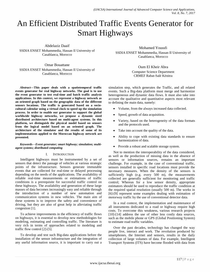
A highway network (Fig. 1) consists of several highways that can be interconnected by exchangers. Each highway is viewed as bidirectional graph. It is described in a single direction by a list of elements representing nodes. For the sake of simplicity Table 1 gives a description of an example of highway part from a given city 1 to city 2, giving the properties of ach node.

Any highway consists of a symmetric set of elements describing it in one direction; it always starts from an entry followed by several intermediate elements and ends in an exit. The second direction is drawn by inverting the input and the output.

Fig. 1. Highway network.

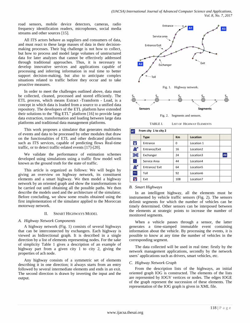
Fig. 2. Segments and sensors.

TABLE I. LIST OF HIGHWAY ELEMENTS

From city 1 to city 2

Type Km Location

Entrance 0 Location 1

Entrance/Exit 16 Location2

Exchanger 24 Location3

Service Area 44 Location4

Entrance/ Exit 64 Location5

Toll 92 Location6

Exit 108 Location7

B. Smart Highways

In an intelligent highway, all the elements must be instrumented by vehicle traffic sensors (Fig. 2). The sensors delimit segments for which the number of vehicles can be timely determined. Other sensors can be interposed between the elements at strategic points to increase the number of monitored segments.

When a vehicle passes through a sensor, the latter generates a time-stamped immutable event containing information about the vehicle. By processing the events, it is possible to know at any time the number of vehicles in the corresponding segment.

The data collected will be used in real time: firstly by the network management applications, secondly by the network users’ applications such as drivers, smart vehicles, etc.

C. Highway Network Graph

From the description lists of the highways, an initial oriented graph IOG is constructed. The elements of the lists are represented by IOGV vertices or nodes. The edges IOGE of the graph represent the succession of these elements. The representation of the IOG graph is given in XML file.


Vol. 8, No. 7, 2017

119 | P a g e


In order to determine all the possible paths from all the entrances of the network to all the possible exits, the IOG must be transformed into a new oriented graph TOG describing the entire network in both directions. The TOG nodes will be represented by TOGV and the edges by TOGE.

From TOG, the Dijkstra Shortest Path Algorithm (DSPA) is performed to determine the list of all possible paths.

As mentioned above, the IOG description is given in an XML file consisting of a collection of vertices and a collection of edges. A vertex is represented by an XML Element “vertex” having the following Attributes:

name: Sensor identifier (ID)

type: Element type (Enumeration)

label: Name of the highway (string)

locality: The locality name of the sensor position (string)

long: Longitude (double)

lat: Latitude (double)

factor: Attendance factor

The edges are represented by the XML Element “edge” having the following Attributes:

source: Source node (IDREF)

target: Destination node (IDREF)

speed: Segment limit speed (double)

distance: Distance between the two nodes (double)

lanes : Number of lanes (int)

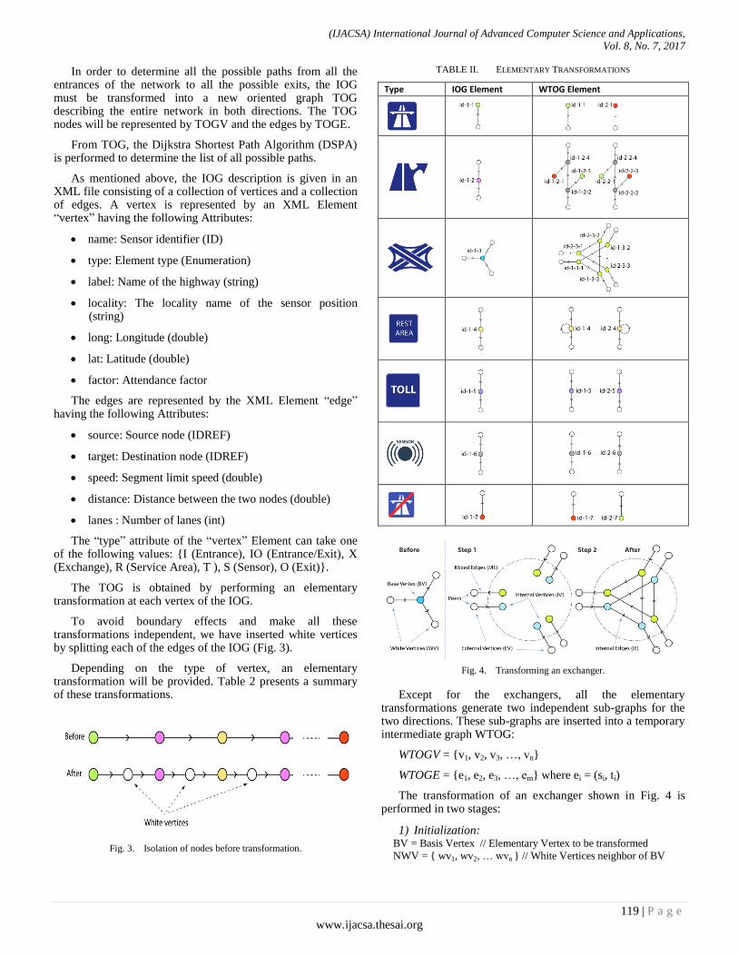
The “type” attribute of the “vertex” Element can take one of the following values: {I (Entrance), IO (Entrance/Exit), X (Exchange), R (Service Area), T ), S (Sensor), O (Exit)}.

The TOG is obtained by performing an elementary transformation at each vertex of the IOG.

To avoid boundary effects and make all these transformations independent, we have inserted white vertices by splitting each of the edges of the IOG (Fig. 3).

Depending on the type of vertex, an elementary transformation will be provided. Table 2 presents a summary of these transformations.

Fig. 3. Isolation of nodes before transformation.

TABLE II. ELEMENTARY TRANSFORMATIONS

Type IOG Element WTOG Element

Fig. 4. Transforming an exchanger.

Except for the exchangers, all the elementary transformations generate two independent sub-graphs for the two directions. These sub-graphs are inserted into a temporary intermediate graph WTOG:

WTOGV = {v1, v2, v3, …, vn}

WTOGE = {e1, e2, e3, …, em} where ei = (si, ti)

The transformation of an exchanger shown in Fig. 4 is performed in two stages:

1) Initialization: BV = Basis Vertex // Elementary Vertex to be transformed

NWV = { wv1, wv2, … wvn } // White Vertices neighbor of BV


Vol. 8, No. 7, 2017

120 | P a g e


EV = {} // External Vertices

ME = {} // Mixed Edges

IV = {} // Internal Vertices

IE = {} // Internal Edges

Stage 1:

For each white vertex wvi from NWV

Create ev1i (Clone of wvi) and insert it into EV,

Create its peer vertex ev2i and insert it into EV

// ev2i represents the sensor for the opposite direction,

Create iv1i (Clone of BV) and insert it into IV,

Create its peer vertex iv2i and insert it into IV,

// iv2i represents the sensor for the opposite direction

IF wvi is successor of BV

Create the edge (iv1i,wv1i) and insert it into ME

Create the edge (wv2i, iv2i) and insert it into ME

Else

Create the edge (wv1i, iv1i) and insert it into ME

Create the edge (iv2i,wv2i) and insert it into ME

End IF

End For

Stage 2:

For each edge mei = (si, ti) in ME

IF ti ϵ IV

For each edge mei = (si, ti) in ME

IF i ≠j and ti not a peer of sj and sj ϵ IV

Create edge (ti, sj) and insert it into IE

End IF

End For

End IF

End For

2) Sub-graph result: WTOGV = UNION(EV, IV)

WTOGE = UNION (ME, IE)

Obtaining the final graph TOG is done by linking the WTOG. This operation consists of removing all the white vertices and restoring the links between the transformed vertices (see Fig. 5).

Finally, we used DSPA to determine all possible paths in the highway network.

Algorithm:

Inputs :

Entries = Vertices of type « I » from TOGV

Exits = Vertices of type « O » from TOGV

Paths = {}

Begin

For each vi from Entries

For each vj from Exits

path := Dijkstra(vi, vj)

IF path is not null

Insert path into Paths

End IF

End For

End

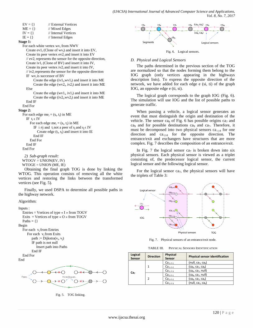
Fig. 5. TOG linking.

Fig. 6. Logical sensors.

D. Physical and Logical Sensors

The paths determined in the previous section of the TOG are normalized so that the nodes forming them belong to the IOG graph (only vertices appearing in the highways description lists). To express the opposite direction of the network, we have added for each edge e (si, ti) of the graph IOG, an opposite edge e (ti, si).

The logical graph corresponds to the graph IOG (Fig. 6). The simulation will use IOG and the list of possible paths to generate traffic.

When passing a vehicle, a logical sensor generates an event that must distinguish the origin and destination of the vehicle. The sensor ca8 of Fig. 6 has possible origins ca7 and ca9 and for possible destinations ca9 and ca7. Therefore, it must be decomposed into two physical sensors ca-1-8 for one direction and ca-2-8 for the opposite direction. The entrance/exit and exchangers have structures that are more complex. Fig. 7 describes the composition of an entrance/exit.

In Fig. 7 the logical sensor ca7 is broken down into six physical sensors. Each physical sensor is viewed as a triplet consisting of, the predecessor logical sensor, the current logical sensor and the following logical sensor.

For the logical sensor ca7, the physical sensors will have the triplets of Table 3:

Fig. 7. Physical sensors of an entrance/exit node.

TABLE III. PHYSICAL SENSORS IDENTIFICATION

Logical Sensor

Direction Physical Sensor

Physical sensor identification

Ca7

1 Ca-1-7-1 (null, ca7, ca8) Ca-1-7-2 (ca6, ca7, ca8) Ca-1-7-3 (ca6, ca7, null)

2 Ca-2-7-1 (ca8, ca7, null) Ca-2-7-2 (ca8, ca7, ca6) Ca-2-7-3 (null, ca7, ca6)


Vol. 8, No. 7, 2017

121 | P a g e


E. Event Model

Depending on the type of sensor, various information can be detected when passing a vehicle. The most common are the speed, the length and the weight of the vehicle. Each time a vehicle passes, an event is generated and a message is sent either directly or via a gateway to an ingestion server. The message must contain at least three basic information; the sensor identifier (previous, current, next), date (Timestamp) and vehicle speed. Here is the general format of the message:

Identifier of predecessor sensor

Identifier of the current sensor

Successor sensor identifier

Timestamp

Speed

Further information about the vehicle depending on the type of sensor.

In the simulation, each vehicle is granted a unique identifier. This makes it possible to track its movement through the highway network.

The simulator is equipped with a virtual clock which allows us to speed up the simulation process. The following section describes the architecture of the proposed simulator.

III. SIMULATOR ARCHITECTURE

A. Overview

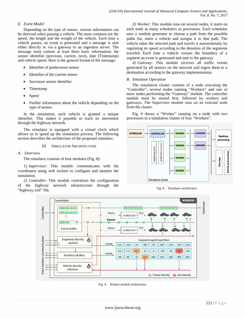
The simulator consists of four modules (Fig. 8):

1) Supervisor: This module communicates with the

coordinator using web sockets to configure and monitor the

simulation.

2) Controller: This module centralizes the configuration

of the highway network infrastructure through the

“highway.xml” file.

3) Worker: This module runs on several nodes, it starts on

each node as many schedulers as processors. Each scheduler

uses a random generator to choose a path from the possible

paths list, starts a vehicle and assigns it to that path. The

vehicle takes the selected path and travels it autonomously by

regulating its speed according to the densities of the segments

traveled. Each time a vehicle crosses the boundary of a

segment an event is generated and sent to the gateway.

4) Gateway: This module receives all traffic events

generated by all sensors on the network and ingest them to a

destination according to the gateway implementation.

B. Simulator Operation

The simulation cluster consists of a node executing the “Controller”, several nodes running “Workers” and one or more nodes performing the “Gateway” module. The controller module must be started first, followed by workers and gateways. The Supervisor module runs on an external node from the cluster.

Fig. 9 shows a “Worker” running on a node with two processors in a simulation cluster of four “Workers”.

Fig. 8. Simulator architecture.

Fig. 9. Worker module architecture.


Vol. 8, No. 7, 2017

122 | P a g e


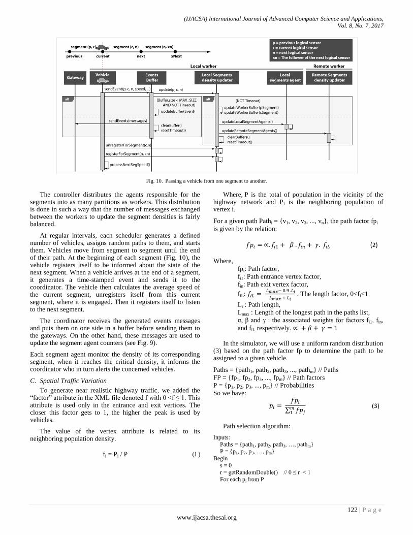
Fig. 10. Passing a vehicle from one segment to another.

The controller distributes the agents responsible for the segments into as many partitions as workers. This distribution is done in such a way that the number of messages exchanged between the workers to update the segment densities is fairly balanced.

At regular intervals, each scheduler generates a defined number of vehicles, assigns random paths to them, and starts them. Vehicles move from segment to segment until the end of their path. At the beginning of each segment (Fig. 10), the vehicle registers itself to be informed about the state of the next segment. When a vehicle arrives at the end of a segment, it generates a time-stamped event and sends it to the coordinator. The vehicle then calculates the average speed of the current segment, unregisters itself from this current segment, where it is engaged. Then it registers itself to listen to the next segment.

The coordinator receives the generated events messages and puts them on one side in a buffer before sending them to the gateways. On the other hand, these messages are used to update the segment agent counters (see Fig. 9).

Each segment agent monitor the density of its corresponding segment, when it reaches the critical density, it informs the coordinator who in turn alerts the concerned vehicles.

C. Spatial Traffic Variation

To generate near realistic highway traffic, we added the “factor” attribute in the XML file denoted f with 0 <f ≤ 1. This attribute is used only in the entrance and exit vertices. The closer this factor gets to 1, the higher the peak is used by vehicles.

The value of the vertex attribute is related to its neighboring population density.

fi = Pi / P

Where, P is the total of population in the vicinity of the highway network and Pi is the neighboring population of vertex i.

For a given path Pathi = {v1, v2, v3, ..., vn}, the path factor fpi

is given by the relation:

(2)

Where,

fpi: Path factor,

fi1: Path entrance vertex factor,

fin: Path exit vertex factor,

fiL:

. The length factor, 0<fi<1

Li : Path length,

Lmax : Length of the longest path in the paths list,

α, β and γ : the associated weights for factors fi1, fin,

and fiL respectively.

In the simulator, we will use a uniform random distribution

(3) based on the path factor fp to determine the path to be assigned to a given vehicle.

Paths = {path1, path2, path3, ..., pathm} // Paths

FP = {fp1, fp2, fp3, ..., fpm} // Path factors

P = {p1, p2, p3, ..., pm} // Probabilities

So we have:

∑

(3)

Path selection algorithm:

Inputs:

Paths = {path1, path2, path3, …, pathm}

P = {p1, p2, p3, …, pm}

Begin

s = 0

r = getRandomDouble() // 0 ≤ r < 1

For each pi from P


Vol. 8, No. 7, 2017

123 | P a g e


IF r ≥ s AND r < s + pi

Return pathi

End IF

s = s + pi

End For

End

D. Temporal Traffic Variation

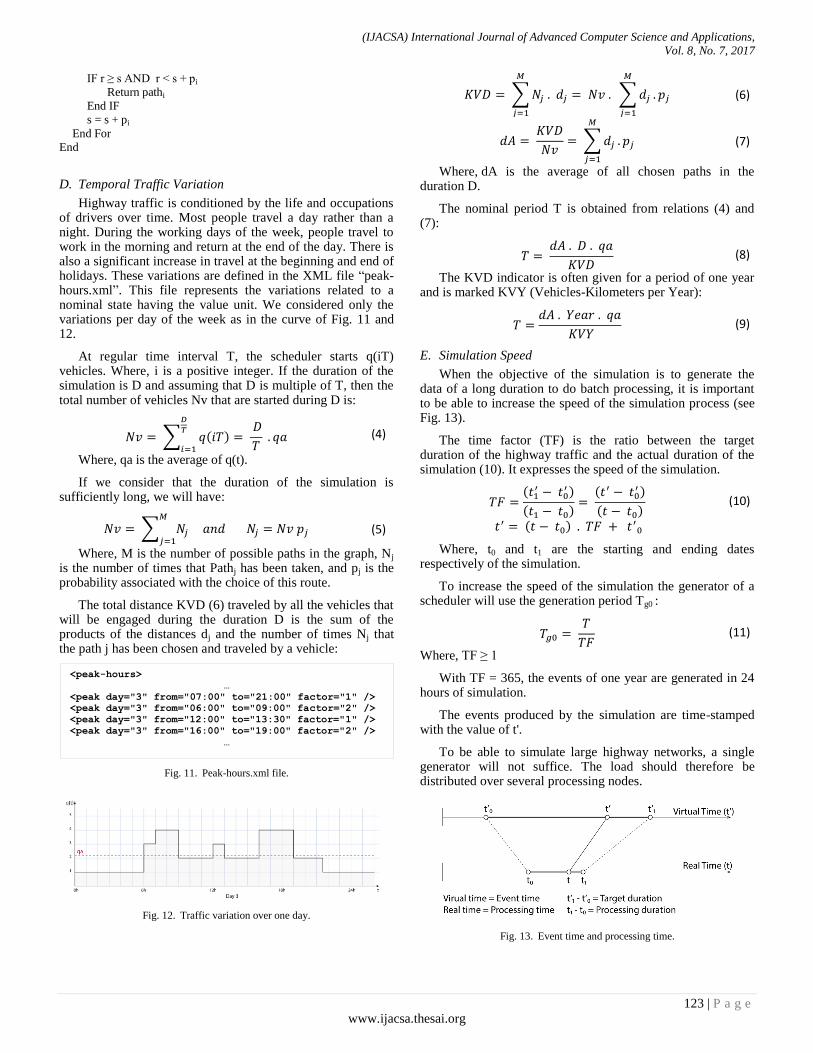
Highway traffic is conditioned by the life and occupations of drivers over time. Most people travel a day rather than a night. During the working days of the week, people travel to work in the morning and return at the end of the day. There is also a significant increase in travel at the beginning and end of holidays. These variations are defined in the XML file “peak-hours.xml”. This file represents the variations related to a nominal state having the value unit. We considered only the variations per day of the week as in the curve of Fig. 11 and 12.

At regular time interval T, the scheduler starts q(iT) vehicles. Where, i is a positive integer. If the duration of the simulation is D and assuming that D is multiple of T, then the total number of vehicles Nv that are started during D is:

∑ ( )

(4)

Where, qa is the average of q(t).

If we consider that the duration of the simulation is sufficiently long, we will have:

∑

(5)

Where, M is the number of possible paths in the graph, Nj is the number of times that Pathj has been taken, and pj is the probability associated with the choice of this route.

The total distance KVD (6) traveled by all the vehicles that will be engaged during the duration D is the sum of the products of the distances dj and the number of times Nj that the path j has been chosen and traveled by a vehicle:

Fig. 11. Peak-hours.xml file.

Fig. 12. Traffic variation over one day.

∑

∑

(6)

∑

(7)

Where, dA is the average of all chosen paths in the duration D.

The nominal period T is obtained from relations (4) and (7):

(8)

The KVD indicator is often given for a period of one year and is marked KVY (Vehicles-Kilometers per Year):

(9)

E. Simulation Speed

When the objective of the simulation is to generate the data of a long duration to do batch processing, it is important to be able to increase the speed of the simulation process (see Fig. 13).

The time factor (TF) is the ratio between the target duration of the highway traffic and the actual duration of the simulation (10). It expresses the speed of the simulation.

(

)

( )

( )

( )

( )

(10)

Where, t0 and t1 are the starting and ending dates respectively of the simulation.

To increase the speed of the simulation the generator of a scheduler will use the generation period Tg0 :

(11)

Where, TF ≥ 1

With TF = 365, the events of one year are generated in 24 hours of simulation.

The events produced by the simulation are time-stamped with the value of t'.

To be able to simulate large highway networks, a single generator will not suffice. The load should therefore be distributed over several processing nodes.

Fig. 13. Event time and processing time.

<peak-hours>

…

<peak day="3" from="07:00" to="21:00" factor="1" />




…


Vol. 8, No. 7, 2017

124 | P a g e


F. Distribution and Load Balancing of Traffic Generators

1) Schedulers distribution In a cluster of N workers nodes each having M processors,

NxM traffic generators can be executed. The load is automatically distributed proportionally using the vehicle commitment period Tg :

(12)

Whenever a vehicle leaves one segment to enter another, it must inform the agents responsible for these two segments. The number of these agents is equivalent to the number of segments of the highway network.

These agents must also be deployed equitably on the N workers nodes.

2) Partitioning and Distributing Segment Agents The agent is responsible for the segments (Fig. 9), must be

partitioned equitably and distributed on all workers in the cluster. A path i is a sequence of one or more segments. A segment belongs to one or more paths. The number of messages arriving at a given segment is related to its frequentation. Knowing the paths probabilities, we can determine the level of attendance at each segment. To do this, we give for each segment (Edge) a weight (ws) which will have the sum of all the probabilities of the paths to which this segment belongs.

The partitioning is done by quasi-balancing the sums of the weights of the segments of each partition.

Initialization:

Amounts = ArrayOfDouble(k)

Partitions = ArrayOfSegments(k)

Segments = {s1, s2, …, sn}

WS = {ws1, ws2, …, wsn}

Begin :

For each Segment sj in Segments

// get the index of the minimum Amounts

index = getMinIndexOf(Amounts)

Insert sj in Partitions[index]

End for End

G. Events Density over Time

When the time factor TF increases, the number of events generated also increases in a given time. It is then important to know in advance this events density (DE) with respect to time (Events/s) in order to size the simulator modules.

∑

(13)

Where, Ncj is the number of sensors in the path j.

H. Vehicle Itinerary

Before entering the highway, the vehicle registers to be informed about the state of the density of the first segment. After a certain delay, the vehicle calculates its speed, determines the duration of the crossing of the segment and starts a timer to warn it at the end of the segment.

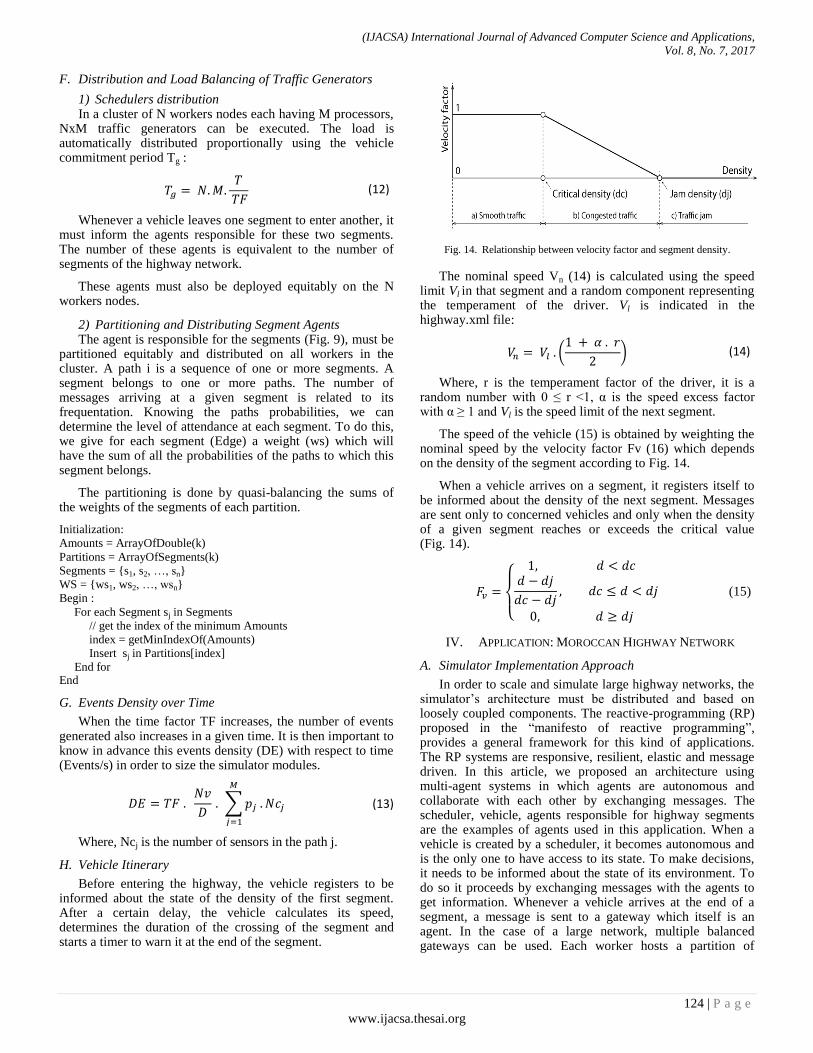
Fig. 14. Relationship between velocity factor and segment density.

The nominal speed Vn (14) is calculated using the speed limit Vl in that segment and a random component representing the temperament of the driver. Vl is indicated in the highway.xml file:

(

) (14)

Where, r is the temperament factor of the driver, it is a random number with 0 ≤ r <1, α is the speed excess factor with α ≥ 1 and Vl is the speed limit of the next segment.

The speed of the vehicle (15) is obtained by weighting the nominal speed by the velocity factor Fv (16) which depends on the density of the segment according to Fig. 14.

When a vehicle arrives on a segment, it registers itself to be informed about the density of the next segment. Messages are sent only to concerned vehicles and only when the density of a given segment reaches or exceeds the critical value (Fig. 14).

{

(15)

IV. APPLICATION: MOROCCAN HIGHWAY NETWORK

A. Simulator Implementation Approach

In order to scale and simulate large highway networks, the simulator’s architecture must be distributed and based on loosely coupled components. The reactive-programming (RP) proposed in the “manifesto of reactive programming”, provides a general framework for this kind of applications. The RP systems are responsive, resilient, elastic and message driven. In this article, we proposed an architecture using multi-agent systems in which agents are autonomous and collaborate with each other by exchanging messages. The scheduler, vehicle, agents responsible for highway segments are the examples of agents used in this application. When a vehicle is created by a scheduler, it becomes autonomous and is the only one to have access to its state. To make decisions, it needs to be informed about the state of its environment. To do so it proceeds by exchanging messages with the agents to get information. Whenever a vehicle arrives at the end of a segment, a message is sent to a gateway which itself is an agent. In the case of a large network, multiple balanced gateways can be used. Each worker hosts a partition of

Vol. 8, No. 7, 2017

125 | P a g e


representative agents of the segments. These agents receive regular messages when vehicles enter or leave their segment. When the density reaches a critical threshold, the agents must inform all vehicles that are about to arrive in that segment.

From a functional point of view, the application must manage a large number of autonomous agents and must be intensive messaging oriented. Since the application is distributed, the data network exchange is also intensive.

Our first implementation of the simulator uses the toolkit Eclipse Vert.x which facilitates the implementation of the RP.

B. Platform Materials

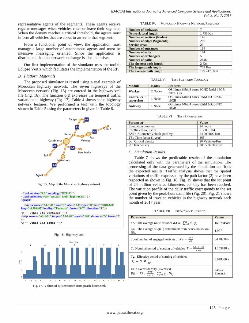
The proposed simulator is tested using a real example of Moroccan highway network. The seven highways of the Moroccan network (Fig. 15) are entered in the highway.xml file (Fig. 16). The function q(t) expresses the temporal traffic variations in highway (Fig. 17). Table 4 shows some highway network features. We performed a test with the topology shown in Table 5 using the parameters in given in Table 6.

Fig. 15. Map of the Moroccan highway network.

Fig. 16. Highway.xml.

Fig. 17. Values of q(t) extracted from peack-hours.xml.

TABLE IV. MOROCCAN HIGHWAY NETWORK FEATURES

Number of highways 7

Network total length 1 736 Km

Number of vertices (Nodes) 146

Number of edges (Segments) 286

Service areas 29

Number of entrances 184

Number of exits 184

Number of exchangers 5

Number of paths 2646

The shortest path length 2 Km

The longest path length 709 Km

The average path length 199.7475 Km

TABLE V. TEST PLATFORM TOPOLOGY

Module Nodes Features

Worker 2 Nodes OS Linux 64bit 8 cores 3GHZ RAM 16GB NIC10GB

Controller + supervisor

1 Node OS Linux 64bit 4 cores RAM 16GB NIC 10GB

Gateway 1 Node OS Linux 64bit 4 cores RAM 16GB NIC 10GB

TABLE VI. TEST PARAMETERS

Parameter Value

Simulation duration 24 hours

Coefficients α, β et γ 0.3, 0.3, 0.4

KVD: Kilometer Vehicle per Day 24 000 000 Km

TF : Time factor (1 year) 365

dc : Critical density 20 Vehicles/Km

jd : Jam density 200 Vehicles/Km

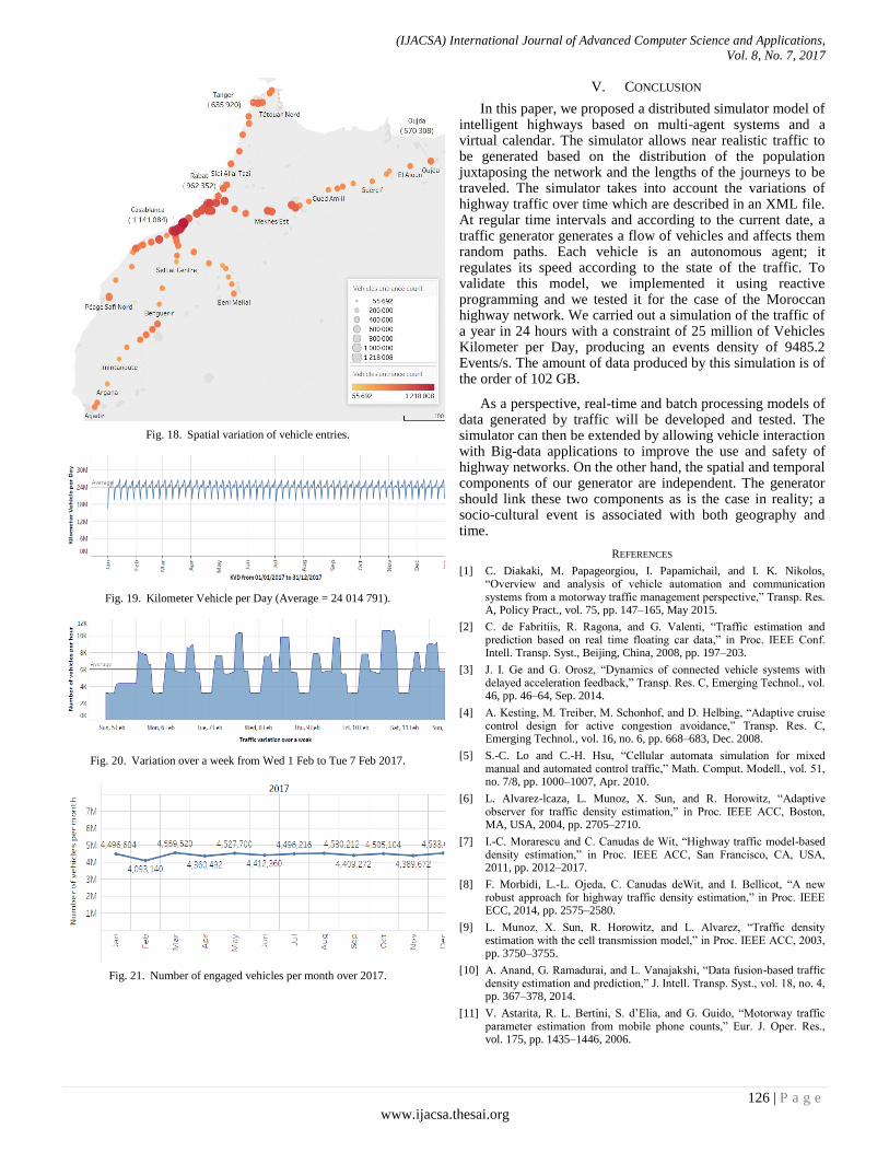
C. Simulation Results

Table 7 shows the predictable results of the simulation calculated only with the parameters of the simulation. The processing of the data generated by the simulation confirms the expected results. Traffic analysis shows that the spatial variations of traffic expressed by the path factor (2) have been respected as shown in Fig. 18. Fig. 19 shows that the set point of 24 million vehicles kilometers per day has been reached. The variation profile of the daily traffic corresponds to the set point given by the peak-hours.xml file (Fig. 20). Fig. 21 shows the number of traveled vehicles in the highway network each month of 2017 year.

TABLE VII. PREDICTABLE RESULTS

Paramètre Valeur

dA : The average route distance ∑ 160.784549

Qa : The average of q(iT) determined from peack-hours.xml file.

1.907

Total number of engaged vehicles :

54 482 847

T, Nominal period of starting of vehicles

1.103818 s

Tg, Effective period of starting of vehicles

0.048386 s

DE : Events density (Events/s)

∑

9485.2 Events/s

<?xml version="1.0" encoding="UTF-8" ?>

<?xml-stylesheet type="text/xsl" href="highway.xsl" ?>

<graph>

<vertex name="A1-1-01" km="9" label="A1" type="O" lat="33.846320"

long="-6.898465" locality="Tamesna" factor="0.7" direction="1" />



<edge source="A1-1-01" target="A1-1-02" speed="120" distance="5" lanes="2"

/>


Vol. 8, No. 7, 2017

126 | P a g e


Fig. 18. Spatial variation of vehicle entries.

Fig. 19. Kilometer Vehicle per Day (Average = 24 014 791).

Fig. 20. Variation over a week from Wed 1 Feb to Tue 7 Feb 2017.

Fig. 21. Number of engaged vehicles per month over 2017.

V. CONCLUSION

In this paper, we proposed a distributed simulator model of intelligent highways based on multi-agent systems and a virtual calendar. The simulator allows near realistic traffic to be generated based on the distribution of the population juxtaposing the network and the lengths of the journeys to be traveled. The simulator takes into account the variations of highway traffic over time which are described in an XML file. At regular time intervals and according to the current date, a traffic generator generates a flow of vehicles and affects them random paths. Each vehicle is an autonomous agent; it regulates its speed according to the state of the traffic. To validate this model, we implemented it using reactive programming and we tested it for the case of the Moroccan highway network. We carried out a simulation of the traffic of a year in 24 hours with a constraint of 25 million of Vehicles Kilometer per Day, producing an events density of 9485.2 Events/s. The amount of data produced by this simulation is of the order of 102 GB.

As a perspective, real-time and batch processing models of data generated by traffic will be developed and tested. The simulator can then be extended by allowing vehicle interaction with Big-data applications to improve the use and safety of highway networks. On the other hand, the spatial and temporal components of our generator are independent. The generator should link these two components as is the case in reality; a socio-cultural event is associated with both geography and time.

REFERENCES

[1] C. Diakaki, M. Papageorgiou, I. Papamichail, and I. K. Nikolos, “Overview and analysis of vehicle automation and communication systems from a motorway traffic management perspective,” Transp. Res. A, Policy Pract., vol. 75, pp. 147–165, May 2015.

[2] C. de Fabritiis, R. Ragona, and G. Valenti, “Traffic estimation and prediction based on real time floating car data,” in Proc. IEEE Conf. Intell. Transp. Syst., Beijing, China, 2008, pp. 197–203.

[3] J. I. Ge and G. Orosz, “Dynamics of connected vehicle systems with delayed acceleration feedback,” Transp. Res. C, Emerging Technol., vol. 46, pp. 46–64, Sep. 2014.

[4] A. Kesting, M. Treiber, M. Schonhof, and D. Helbing, “Adaptive cruise control design for active congestion avoidance,” Transp. Res. C, Emerging Technol., vol. 16, no. 6, pp. 668–683, Dec. 2008.

[5] S.-C. Lo and C.-H. Hsu, “Cellular automata simulation for mixed manual and automated control traffic,” Math. Comput. Modell., vol. 51, no. 7/8, pp. 1000–1007, Apr. 2010.

[6] L. Alvarez-lcaza, L. Munoz, X. Sun, and R. Horowitz, “Adaptive observer for traffic density estimation,” in Proc. IEEE ACC, Boston, MA, USA, 2004, pp. 2705–2710.

[7] I.-C. Morarescu and C. Canudas de Wit, “Highway traffic model-based density estimation,” in Proc. IEEE ACC, San Francisco, CA, USA, 2011, pp. 2012–2017.

[8] F. Morbidi, L.-L. Ojeda, C. Canudas deWit, and I. Bellicot, “A new robust approach for highway traffic density estimation,” in Proc. IEEE ECC, 2014, pp. 2575–2580.

[9] L. Munoz, X. Sun, R. Horowitz, and L. Alvarez, “Traffic density estimation with the cell transmission model,” in Proc. IEEE ACC, 2003, pp. 3750–3755.

[10] A. Anand, G. Ramadurai, and L. Vanajakshi, “Data fusion-based traffic density estimation and prediction,” J. Intell. Transp. Syst., vol. 18, no. 4, pp. 367–378, 2014.

[11] V. Astarita, R. L. Bertini, S. d’Elia, and G. Guido, “Motorway traffic parameter estimation from mobile phone counts,” Eur. J. Oper. Res., vol. 175, pp. 1435–1446, 2006.


Vol. 8, No. 7, 2017

127 | P a g e


[12] J. C. Herrera et al., “Evaluation of traffic data obtained via GPS-enabled mobile phones: The Mobile Century field experiment,” Transp. Res. C, Emerging Technol., vol. 18, no. 4, pp. 568–583, Aug. 2010.

[13] W. Deng, H. Lei, and X. Zhou, “Traffic state estimation and uncertainty quantification based on heterogeneous data sources: A three detector approach,” Transp. Res. B, Methodol., vol. 57, pp. 132–157, Nov. 2013.

[14] T. Seo, T. Kusakabe, and Y. Asakura, “Estimation of flow and density using probe vehicles with spacing measurement equipment,” Transp. Res. C, vol. 53, pp. 134–150, Apr. 2015.

[15] J. Fiosina, M. Fiosins and J. Müller, "Big Data Processing and Mining for Next Generation Intelligent Transportation Systems," Jurnal Teknologi, vol. 63, no. 3, pp. 21-38, 2013.

[16] J. Caserta and E. Cordo, "Big ETL: The Next 'Big' Thing," 9 February 2015. http://data-informed.com/big-etl-next-bigthing/.

[17] Q. Ou, R. L. Bertini, J. W. C. van Lint, and S. P. Hoogendoorn, “A theoretical framework for traffic speed estimation by fusing low-resolution probe vehicle data,” IEEE Trans. Intell. Transp. Syst., vol. 12, no. 3, pp. 747–756, Sep. 2011.

[18] M. Papageorgiou and A. Messmer, “METANET: A macroscopic simulation program for motorway networks,” Traffic Eng. Control, vol. 31, no. 9, pp. 466–470, 1990.

[19] V. Punzo, M. T. Borzacchiello, and B. Ciuffo, “On the assessment of vehicle trajectory data accuracy and application to the Next Generation SIMulation (NGSIM) program data,” Transp. Res. C, Emerging Technol., vol. 19, no. 6, pp. 1243–1262, Dec. 2011.

[20] “Next Generation SIMulation (NGSIM),” U.S. Dept. Transp., Washington, DC, USA, 2005. Available: www.ngsimcommunity.

an efficient distributed traffic events generator for ... · an efficient distributed traffic...

Documents