An efficient GVNS for solving TravelingSalesman Problem with Time Windows

Nenad Mladenovic a,1 Raca Todosijevic b,2 Dragan Urosevic b,3

a Department of Mathematics, SISCM, Brunel University, London, UK

b Mathematical Instutute, Serbian Academy of Sciences and Arts, Belgrade, Serbia

Abstract

Although GVNS is shown to be powerful and robust method for solving travelingsalesman and vehicle routing problems, its efficient implementation may play sig-nificant role in solving large size instances. In this paper we suggest new GVNSheuristic for solving TSPTW. It uses more efficient data structure, different neigh-borhoods, new efficient feasibility checking procedure, for example, than a recentGVNS method [3], that may be considered as a state-of-the-art heuristic. As a re-sult, our GVNS is significantly faster than previous GVNS and therefore is able toimprove 14 out of 25 best known solutions for large test instances from the literature.

Keywords: Traveling Salesman Problem, Time window, GVNS.

1 Introduction

The Traveling Salesman Problem with Time Windows (TSPTW) is a variantof the well-known Traveling Salesman Problem (TSP). Suppose that is given a

1 Email: Nenad.Mladenovic@brunel.ac.uk2 Email: racatodosijevic@gmail.com3 Email: draganu@turing.mi.sanu.ac.rs

Available online at www.sciencedirect.com

Electronic Notes in Discrete Mathematics 39 (2012) 83–90

1571-0653/$ – see front matter © 2012 Elsevier B.V. All rights reserved.

www.elsevier.com/locate/endm

doi:10.1016/j.endm.2012.10.012

depot and a set of customers (each customer has its service time (i.e. the timethat must be spent at the customer) and a time window defining its readytime and due date). The TSPTW problem consists in finding a minimumcost tour starting and ending on a given depot, visiting each customer exactlyonce before its due date. The traveling salesman is allowed to arrive at somecustomer before its ready time, but in that case the traveling salesman hasto wait. Obviously, there are some tours which do not allow the travelingsalesman to respect due dates of all customers, therefore all such tours wewill call infeasible tours (solutions), while all others we will call feasible tours(solutions). The cost of a tour is the total distance traveled.

Suppose that is given graph G = (V,A), where V = {1, 2, . . . , n}, 0 isdepot and A = {(i, j) : i, j ∈ V ∪ {0}} is the set of arcs between customers.The cost of traveling from i to j is represented by cij that includes both theservice time of customer i and the time needed to travel from i to j. Eachcustomer i has an associated time window [ai, bi], where ai and bi representthe ready time and due date, respectively. So, Traveling Salesman Problemwith Time windows can be stated, mathematically, as a problem of finding aHamiltonian tour starting from the depot, that satisfies all time windows andminimizes the total distance traveled.

TSPTW is NP −hard problem since it is a special case of the well-knownTraveling Salesman Problem which is NP − hard problem. Because of thatthere is a need for a heuristic which will be able to solve efficiently realisticinstances in the reasonable amount of time. In that direction, some steps havebeen already made. For example, Carlton and Barnes [2] use a tabu-searchheuristic with a static penalty function, that considers infeasible solutions.Gendreau et al. [4] propose a insertion heuristic based on GENIUS [4] thatgradually builds the route and improves it in a post-optimization phase basedon successive removal and reinsertion of nodes. Calvo[1] solves an assignmentproblem with an ad hoc objective function and builds a feasible tour mergingall found sub-tours into a main tour, then applies a 3-opt local search proce-dure [5] to improve the initial feasible solution. Ohlmann and Thomas [8] usea variant of simulated annealing ,called compressed annealing, that relaxesthe time windows constraints by integrating a variable penalty method withina stochastic search procedure. Two new heuristic were proposed in 2010. Oneheuristic was proposed by Blum et al. [6], while the other was proposed byUrrutia et al. [3] These two heuristics are, currently, the state of the artheuristics.

In this paper we propose new two stage VNS based heuristic for solvingthe TSPTW problem. At the first stage we use VNS to obtain feasible initial

N. Mladenovic et al. / Electronic Notes in Discrete Mathematics 39 (2012) 83–9084

solution, while at the second we use GVNS to improve an initial solutionobtained at the previous stage. The proposed GVNS is more efficient thanthat proposed in [3], since our GVNS offers some new best known solutionsand since it consumes less computational time in mean.

The rest of the paper is organized as follows. In Section 2, we describeimplementation issues of GVNS heuristic, while in Section 3 we present com-putational results. Finally, in Section 4 we give some concluding remarks.

2 GVNS for TSPTW

2.1 Building an initial solution

Building an initial solution is also NP-hard, so we decide to use the procedurewhich was proposed in [3]. That procedure is VNS based procedure whichrelocates customers of a random solution until a feasible solution is obtained.

2.2 Neighborhood structures

Most common moves which are performed on some TSP solution are 2-optmoves and OR-opt moves. The 2-opt move breaks down two edges of currentsolution and make two new edges inverting part of solution in such way thatresulting solution is still a tour. One variant of 2-opt move is so-called 1-optmove which is applicable on four consecutive customers, i.e. i1, i2, i3 and i4in such way that edges i1i2 and i3i4 are broken down while the edge i2i3 isinverted. On the other hand, OR-opt move relocate a chain of consecutivecustomers without inverting any part of a solution. If a chain contains kcustomers, we will call such move OR-opt-k move. If a chain of k consecutivecustomers is moved backward that move will be called backward OR-opt-k.Similarly, if a chain is moved forward, the move will be called forward OR-opt-k.

Previously described moves can be performed on each feasible solutionof TSPTW problem since TSPTW is a variant of TSP. However, we must becareful because some moves can lead to infeasible solutions. So, it is importantto check whether some move yields feasible or infeasible solution. For thatpurpose we build an array named Gap where Gap[i] denotes maximal value forwhich arrival time at node i, i.e. βi, could be increased so that the feasibility onthe final part of a tour, which starts at node i, is kept. Elements of array Gapare evaluated starting at depot and moving backward through a tour. If wesuppose that node j precede node i than Gap[j] is calculated in the followingway: Gap[j] = min(Gap[i] +max(0, aj − βj), bj − βj) where Gap[0] = b0− β0.

N. Mladenovic et al. / Electronic Notes in Discrete Mathematics 39 (2012) 83–90 85

If we want to check feasibility of some move we have to recalculate arrival timeat each customer between the first and the last customer involved in move aswell as at these two nodes (first and last customer according to resulting tourif the move would be performed). If all those customers are still non-violatedand arrival time at last customer involved in move is increased for value lessor equal to its gap value then new solution will be feasible otherwise it will beinfeasible.

In our VND procedure we decide to explore the following neighborhoodstructures respectively: 1-opt, backward OR-opt-2, forward OR-opt-2, back-ward OR-opt-1, forward OR-opt-1, 2-opt. Since each move could be consideredas a relocation of some customer, we decide to explore neighborhood structuresmoving some customer, i.e. i, j(j = 1, 2, 3, ..) positions backward or forwarddepending on examined neighborhood structure. However, the search for animprovement moving customer i in some neighborhood structure is stoppedas soon as we find some infeasible move (move which does not keep feasibilityof solution) that reduces the value of the objective function.

Each of those neighborhood structures is explored using the best improve-ment search strategy. However, the search for an improvement of a currentsolution is continued in the next neighborhood structure whether we find animprovement in some neighborhood structure or not. The whole search pro-cedure is repeated until there is an improvement of a current solution in someneighborhood structure.

2.3 Shaking procedure

As a shaking procedure we use a function named Perturbation(X, level) [3]which performs level random feasible OR-opt-1 moves on given solution X.

2.4 The scheme of GVNS

Applying rules of GVNS [7] we obtain GVNS for TSPTW which steps aregiven in Algorithm 1.

N. Mladenovic et al. / Electronic Notes in Discrete Mathematics 39 (2012) 83–9086

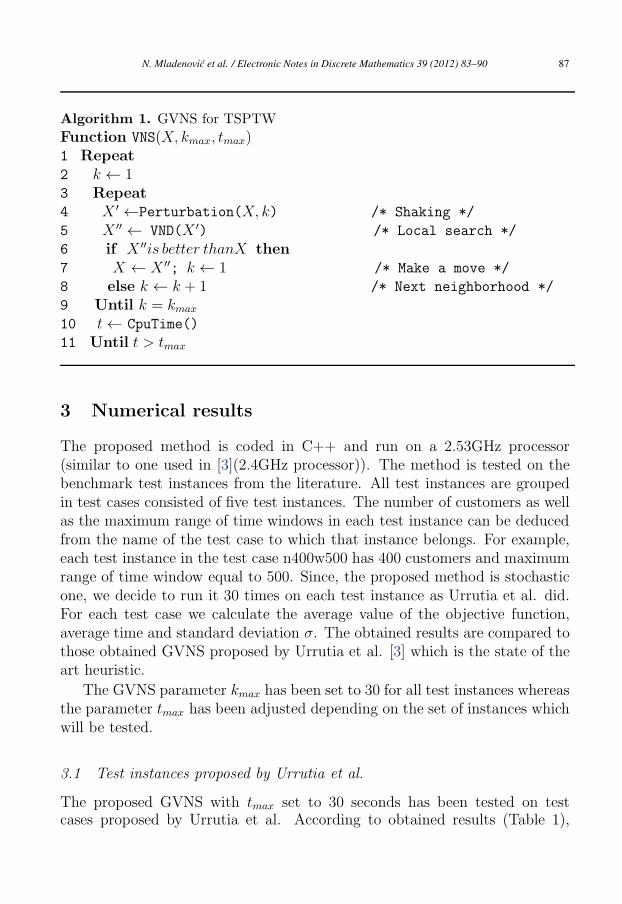
Algorithm 1. GVNS for TSPTW

Function VNS(X, kmax, tmax)1 Repeat2 k ← 13 Repeat4 X ′ ←Perturbation(X, k) /* Shaking */

5 X ′′ ← VND(X ′) /* Local search */

6 if X ′′is better thanX then7 X ← X ′′; k ← 1 /* Make a move */

8 else k ← k + 1 /* Next neighborhood */

9 Until k = kmax

10 t← CpuTime()

11 Until t > tmax

3 Numerical results

The proposed method is coded in C++ and run on a 2.53GHz processor(similar to one used in [3](2.4GHz processor)). The method is tested on thebenchmark test instances from the literature. All test instances are groupedin test cases consisted of five test instances. The number of customers as wellas the maximum range of time windows in each test instance can be deducedfrom the name of the test case to which that instance belongs. For example,each test instance in the test case n400w500 has 400 customers and maximumrange of time window equal to 500. Since, the proposed method is stochasticone, we decide to run it 30 times on each test instance as Urrutia et al. did.For each test case we calculate the average value of the objective function,average time and standard deviation σ. The obtained results are compared tothose obtained GVNS proposed by Urrutia et al. [3] which is the state of theart heuristic.

The GVNS parameter kmax has been set to 30 for all test instances whereasthe parameter tmax has been adjusted depending on the set of instances whichwill be tested.

3.1 Test instances proposed by Urrutia et al.

The proposed GVNS with tmax set to 30 seconds has been tested on testcases proposed by Urrutia et al. According to obtained results (Table 1),

N. Mladenovic et al. / Electronic Notes in Discrete Mathematics 39 (2012) 83–90 87

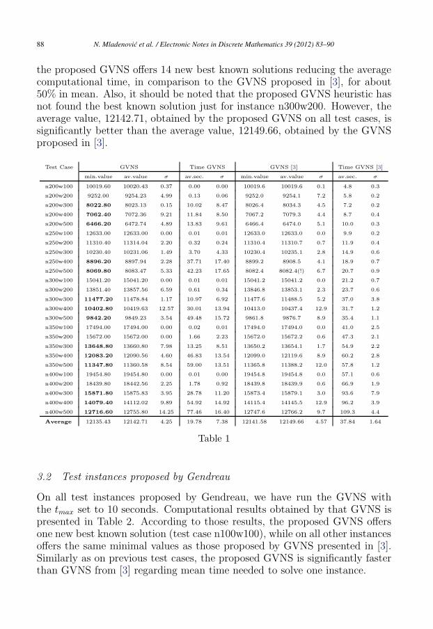
the proposed GVNS offers 14 new best known solutions reducing the averagecomputational time, in comparison to the GVNS proposed in [3], for about50% in mean. Also, it should be noted that the proposed GVNS heuristic hasnot found the best known solution just for instance n300w200. However, theaverage value, 12142.71, obtained by the proposed GVNS on all test cases, issignificantly better than the average value, 12149.66, obtained by the GVNSproposed in [3].

Test Case GVNS Time GVNS GVNS [3] Time GVNS [3]

min.value av.value σ av.sec. σ min.value av.value σ av.sec. σ

n200w100 10019.60 10020.43 0.37 0.00 0.00 10019.6 10019.6 0.1 4.8 0.3

n200w200 9252.00 9254.23 4.99 0.13 0.06 9252.0 9254.1 7.2 5.8 0.2

n200w300 8022.80 8023.13 0.15 10.02 8.47 8026.4 8034.3 4.5 7.2 0.2

n200w400 7062.40 7072.36 9.21 11.84 8.50 7067.2 7079.3 4.4 8.7 0.4

n200w500 6466.20 6472.74 4.89 13.83 9.61 6466.4 6474.0 5.1 10.0 0.3

n250w100 12633.00 12633.00 0.00 0.01 0.01 12633.0 12633.0 0.0 9.9 0.2

n250w200 11310.40 11314.04 2.20 0.32 0.24 11310.4 11310.7 0.7 11.9 0.4

n250w300 10230.40 10231.06 1.49 3.70 4.33 10230.4 10235.1 2.8 14.9 0.6

n250w400 8896.20 8897.94 2.28 37.71 17.40 8899.2 8908.5 4.1 18.9 0.7

n250w500 8069.80 8083.47 5.33 42.23 17.65 8082.4 8082.4(!) 6.7 20.7 0.9

n300w100 15041.20 15041.20 0.00 0.01 0.01 15041.2 15041.2 0.0 21.2 0.7

n300w200 13851.40 13857.56 6.59 0.61 0.34 13846.8 13853.1 2.3 23.7 0.6

n300w300 11477.20 11478.84 1.17 10.97 6.92 11477.6 11488.5 5.2 37.0 3.8

n300w400 10402.80 10419.63 12.57 30.01 13.94 10413.0 10437.4 12.9 31.7 1.2

n300w500 9842.20 9849.23 3.54 49.48 15.72 9861.8 9876.7 8.9 35.4 1.1

n350w100 17494.00 17494.00 0.00 0.02 0.01 17494.0 17494.0 0.0 41.0 2.5

n350w200 15672.00 15672.00 0.00 1.66 2.23 15672.0 15672.2 0.6 47.3 2.1

n350w300 13648.80 13660.80 7.98 13.25 8.51 13650.2 13654.1 1.7 54.9 2.2

n350w400 12083.20 12090.56 4.60 46.83 13.54 12099.0 12119.6 8.9 60.2 2.8

n350w500 11347.80 11360.58 8.54 59.00 13.51 11365.8 11388.2 12.0 57.8 1.2

n400w100 19454.80 19454.80 0.00 0.01 0.00 19454.8 19454.8 0.0 57.1 0.6

n400w200 18439.80 18442.56 2.25 1.78 0.92 18439.8 18439.9 0.6 66.9 1.9

n400w300 15871.80 15875.83 3.95 28.78 11.20 15873.4 15879.1 3.0 93.6 7.9

n400w400 14079.40 14112.02 9.89 54.92 14.92 14115.4 14145.5 12.9 96.2 3.9

n400w500 12716.60 12755.80 14.25 77.46 16.40 12747.6 12766.2 9.7 109.3 4.4

Average 12135.43 12142.71 4.25 19.78 7.38 12141.58 12149.66 4.57 37.84 1.64

Table 1

3.2 Test instances proposed by Gendreau

On all test instances proposed by Gendreau, we have run the GVNS withthe tmax set to 10 seconds. Computational results obtained by that GVNS ispresented in Table 2. According to those results, the proposed GVNS offersone new best known solution (test case n100w100), while on all other instancesoffers the same minimal values as those proposed by GVNS presented in [3].Similarly as on previous test cases, the proposed GVNS is significantly fasterthan GVNS from [3] regarding mean time needed to solve one instance.

N. Mladenovic et al. / Electronic Notes in Discrete Mathematics 39 (2012) 83–9088

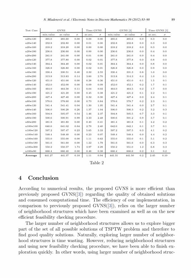
Test Case GVNS Time GVNS GVNS [3] Time GVNS [3]

min.value av.value σ av.sec. σ min.value av.value σ av.sec. σ

n20w120 265.6 265.60 0.00 0.00 0.00 265.6 265.6 0.0 0.3 0.0

n20w140 232.8 232.80 0.00 0.01 0.00 232.8 232.8 0.0 0.3 0.0

n20w160 218.2 218.20 0.00 0.00 0.00 218.2 218.2 0.0 0.3 0.0

n20w180 236.6 236.60 0.00 0.00 0.00 236.6 236.6 0.0 0.4 0.0

n20w200 241.0 241.00 0.00 0.01 0.00 241.0 241.0 0.0 0.4 0.0

n40w120 377.8 377.80 0.00 0.02 0.01 377.8 377.8 0.0 0.8 0.0

n40w140 364.4 364.40 0.00 0.02 0.01 364.4 364.4 0.0 0.8 0.0

n40w160 326.8 326.80 0.00 0.02 0.01 326.8 326.8 0.0 0.9 0.0

n40w180 330.4 330.51 0.40 2.22 2.55 330.4 331.3 0.8 1.0 0.0

n40w200 313.8 313.83 0.14 3.60 2.70 313.8 314.3 0.4 1.0 0.1

n60w120 451.0 451.00 0.00 0.28 0.36 451.0 451.0 0.1 1.5 0.1

n60w140 452.0 452.00 0.00 0.09 0.09 452.0 452.1 0.2 1.7 0.1

n60w160 464.0 464.58 0.11 0.04 0.02 464.0 464.5 0.2 1.7 0.0

n60w180 421.2 421.20 0.00 0.45 0.38 421.2 421.2 0.1 2.2 0.1

n60w200 427.4 427.40 0.00 0.32 0.30 427.4 427.4 0.0 2.4 0.1

n80w100 578.6 578.60 0.00 0.73 0.84 578.6 578.7 0.2 2.3 0.1

n80w120 541.4 541.41 0.04 1.30 1.95 541.4 541.4 0.0 2.7 0.1

n80w140 506.0 506.28 0.26 1.37 1.04 506.0 506.3 0.2 3.2 0.3

n80w160 504.8 505.07 0.54 1.46 2.37 504.8 505.5 0.7 3.3 0.1

n80w180 500.6 500.91 0.99 3.33 2.48 500.6 501.2 0.9 3.7 0.1

n80w200 481.8 481.80 0.00 0.40 0.41 481.4 481.8 0.1 4.2 0.2

n100w100 640.6 641.02 0.64 2.79 2.40 642.0 642.1 0.1 3.7 0.1

n100w120 597.2 597.47 0.23 5.65 3.33 597.2 597.5 0.3 4.1 0.2

n100w140 548.4 548.40 0.00 0.23 0.07 548.4 548.4 0.0 4.4 0.2

n100w160 555.0 555.00 0.00 1.11 0.62 555.0 555.0 0.1 5.1 0.2

n100w180 561.6 561.60 0.00 1.22 1.78 561.6 561.6 0.0 6.3 0.3

n100w200 550.2 550.57 1.74 3.97 2.29 550.2 551.0 1.2 6.8 0.3

n100w80 666.4 666.40 0.00 0.46 0.38 666.4 666.6 0.2 3.1 0.2

Average 441.27 441.37 0.18 1.11 0.94 441.31 441.50 0.2 2.45 0.10

Table 2

4 Conclusion

According to numerical results, the proposed GVNS is more efficient thanpreviously proposed GVNS([3]) regarding the quality of obtained solutionsand consumed computational time. The efficiency of our implementation, incomparison to previously proposed GVNS([3]), relies on the larger numberof neighborhood structures which have been examined as well as on the newefficient feasibility checking procedure.

The larger number of neighborhood structures allows us to explore biggerpart of the set of all possible solutions of TSPTW problem and therefore tofind good quality solutions. Naturally, exploring larger number of neighbor-hood structures is time wasting. However, reducing neighborhood structuresand using new feasibility checking procedure, we have been able to finish ex-ploration quickly. In other words, using larger number of neighborhood struc-

N. Mladenovic et al. / Electronic Notes in Discrete Mathematics 39 (2012) 83–90 89

tures, reducing neighborhood structures and introducing new way to checkfeasibility of some move, we have made compromise between solution qualityand computational time to obtain that solution.

References

[1] Calvo, R. W., A new heuristic for the traveling salesman problem with timewindows, Transportation Science 34 (2000), 113–124.

[2] Carlton, W. B., and J. W. Barnes, Solving the travelling salesman problemwith time windows using tabu search, IEEE Transactions 28 (1996), 617–629.

[3] Da Silva, R. F., and S. Urrutia, A General VNS heuristic for the travelingsalesman problem with time windows, Discrete Optimization 7 (2010), 203–211.

[4] Gendreau, M., A. Hertz, G. Laporte, and M. Stan, A generalized insertionheuristic for the traveling salesman problem with time windows, OperationResearch 46 (1998), 330–335.

[5] Johnson, D. S., and L. A. McGeoch, The traveling salesman problem: a casestudy in local optimization, in: Aarts, E. H. L., and J. K. Lenstra(Eds.), LocalSearch in Combinatorial Optimization, John Wiley and Sons (1995), 215–310.

[6] Lopez-Ibanez, M., C. Blum, Beam-ACO for the travelling salesman problemwith time windows, Computers and Operations Research 37 (2010), 1570–1583.

[7] Mladenovic, N., and P. Hansen, Variable neighborhood search, Computers andOperations Research 24 (1997), 1097–1100.

[8] Ohlmann, J. W., B. W. Thomas, A compressed-annealing heuristic forthe traveling salesman problem with time windows, INFORMS Journal onComputing 19 (2007), 80–90.

N. Mladenovic et al. / Electronic Notes in Discrete Mathematics 39 (2012) 83–9090