an efficient similarity measure technique for medical image

Sadhana Vol. 37, Part 6, December 2012, pp. 709–721. c© Indian Academy of Sciences

An efficient similarity measure technique for medical imageregistration

VILAS H GAIDHANE1,∗, YOGESH V HOTE2 andVIJANDER SINGH1

1Department of Instrumentation and Control Engineering,Netaji Subhas Institute of Technology, University of Delhi, New Delhi, 110 078 India2Department of Electrical Engineering, Indian Institute of Technology, Roorkee,247 667 Indiae-mail: [email protected]; [email protected]

MS received 19 January 2012; revised 31 July 2012; accepted 6 September 2012

Abstract. In this paper, an efficient similarity measure technique is proposed formedical image registration. The proposed approach is based on the Gerschgorincircles theorem. In this approach, image registration is carried out by consideringGerschgorin bounds of a covariance matrix of two compared images with normal-ized energy. The beauty of this approach is that there is no need to calculate imagefeatures like eigenvalues and eigenvectors. This technique is superior to other well-known techniques such as normalized cross-correlation method and eigenvalue-basedsimilarity measures since it avoids the false registration and requires less computation.The proposed approach is sensitive to small defects and robust to change in illumina-tions and noise. Experimental results on various synthetic medical images have shownthe effectiveness of the proposed technique for detecting and locating the disease inthe complicated medical images.

Keywords. Gerschgorin circle; Gerschgorin bound; covariance matrix;eigenvalues; normalized cross-correlation; magnetic resonance images (MRI).

1. Introduction

Image registration is one of the fundamental tasks required in many image processing applica-tions. It is the process of matching two data sets or images taken from the same scene recorded atdifferent time intervals, locations, viewpoints, illuminations and sensors. It is an important pro-cess which involves four steps: feature detection, feature matching, transform model estimation

∗For correspondence

709

710 Vilas H Gaidhane et al

and image resampling. Particularly, image registration is required in multispectral classification,changed detection, environmental monitoring, remote sensing, geographic information system(GIS), weather forecasting, defect detection in material, computer vision and computer tomog-raphy (CT) scanning, etc. (Zitová & Flusser 2003; Jung & Im 2011). In recent years, due to thefast growth of advanced data acquisition systems, researchers develop a keen interest in the fieldof automatic image registration.

Feature matching is the main step in image registration system. In this process, the detectedfeatures in the reference image and the scene image are matched using the image pixels inten-sity value. There are two basic methods: area-based methods and feature-based methods whichare used for image feature matching in image registration. Area-based method is called as acorrelation method or template matching method. These methods use to match the windows ofpredefined size (smaller than the reference image) for correspondence estimation (Andronache etal 2008). If the computational speed is the main concern and images are acquired under varyingconditions, then Fourier methods are more suitable for image registration. An adaptable multi-layer fractional Fourier transform approach which is also a area-based method, introduced byPan et al (2009) for image registration. Suppose, S(x ,y) and R(x ,y) are scene image and refer-ence image, respectively, then their corresponding Fourier transforms are S(ξ , η) and R(ξ , η),respectively. The cross power spectrum of these two images is given as (Zitová & Flusser 2003),

S(ξ, η)R(ξ, η)

|S(ξ, η)R(ξ, η)| = e− j2π(ξ x0−ηy0). (1)

If variation in the image is present, then images can be registered using the combination ofPolar-log mapping and the phase correlation (Zheng et al 2003). Viola & Wells (1997) proposedmutual information (MI) method describes the application of the mutual information for the reg-istration using the magnetic resonance images (MRI) and 3D object model matching. Such MImethods found applications to register MR-PET and MR-CT images of a human brain. It workswith the entire data and intensity of the images. Recently, a multimodal image registration, aleading technique is introduced by Lu et al (2008) to solve medical imaging. In these tech-niques, mutual information method is used to measure the statistical dependencies between twoimages. The mutual information between two random variables p and q is given as (Zitová &Flusser 2003),

M(p, q) = H(p) + H(q) − H(p, q), (2)

where, H(p) is the entropy of the random variables. However, these methods suffer from theproblems introduced by the local noises, illuminations and deviations. To avoid these complexi-ties, a simple and new method for medical image registration using the concept of Gerschgorincircle theorem (Gerschgorin 1931) is proposed. Recently, this theorem has been used in variousengineering applications (Hote et al 2006, 2011; Hote 2009; Gaidahne et al 2012). This workhas been motivated due to the need of effective matching or mismatching measure between twocompared images in the presence of local distortions.

The rest of the paper is organised as follows: A brief overview of existing correlation matchingmethods is presented in section 2. Section 3 describes a basic Gerschgorin circle theorem and itsbounds. The proposed approach for medical image registration is presented in section 4. Exper-imentation results and discussions are presented in section 5. Finally, conclusions are drawn insection 6.

Efficient similarity measure for image registration 711

2. Normalized cross-correlation and eigenvalue-based image matching

The similarity measure between two uncalibrated images say R(x , y) and S(x , y), is defined asthe normalized cross-correlation which is given as (Andronache et al 2008)

μ =

m∑

x=−m

n∑

y=−n

[R(x, y) − R

] · [S(x, y) − S

]

(2m + 1) (2n + 1) σ (R) σ (S), (3)

where μ is the normalized cross-correlation, R and S is the average pixel value and σ (R) andσ (S) is the standard deviation of the elements in R and S images, respectively. This similaritymeasure is computed for windowed region pairs for which the maximum value ‘1’ is set asmatching result. For dissimilar windowed region, the value of cross-correlation also approachesto unity. Therefore, the false decision on the similarity is possible. However, if the referenceimage is deformed by more complex transformation, then the window is not able to match thesame part of the scene image in the reference image. However, the cross-correlation methodis more popular due to its simple hardware implementation, which makes useful for real timeapplications (Lindoso & Entrena 2007).

Tsai & Yang (2005) proposed an eigenvalue-based similarity measure which applied suc-cessfully for defect detection. This method is mainly responsive to local deviations in images.Moreover, this approach is based on the shape of the pair wise gray-level distribution of the twoimages. Suppose, s(p, q) and r(p, q) are the gray-levels of scene image and reference image,respectively, then the pair-wise gray values at coincident pixel locations in the s and r imagesare used as the coordinates to plot the correspondence map. For similar images, map is a straightline and it disperses away from straight line for dissimilar images. The shape of the straight linein the map is obtained from the statistical and geometrical properties of the covariance matrixwhich is calculated from two compared images. For any size of images, the resultant covariancematrix A is of the order 2 × 2 which is given as

A =[

a11 a12a21 a22

]

. (4)

The resultant covariance matrix is positive and symmetric. It has two eigenvalues, first is calledas the smallest eigenvalue λS and second is called as the largest eigenvalue λL . Mathematically,these eigenvalues can be obtained using the elements of covariance matrix A, which are given as(Tsai & Yang 2005; Sun et al 2008),

λS = 1

2

[

a11 + a22 −√

(a11 − a22)2 + 4a2

12

]

(5)

λL = 1

2

[

a11 + a22 +√

(a11 − a22)2 + 4a2

12

]

, (6)

where λS ≤ λL . If two compared images are identical then the shape of correspondence map is astraight line and the variation along the minor axis is zero. Thus, value of the smallest eigenvalueideally zero if scene image and reference image is identical. The value λS increases and becomesvery large as the dissimilarity between two images increases. Thus, the similarity between ref-erence image and scene image can be evaluated using the smallest eigenvalue. In this method,the selection of sub-image window size is an important issue. The performance of system is


affected with small as well as the large size of sub-image window regions. This method is stillsuperior than the area-based registration method such as normalized cross-correlation (NCC). InNormalized cross-correlation method, the value of NCC is close to ‘1’ for two similar as wellas dissimilar images. Therefore, it is very difficult to decide the similarity and dissimilarity ofthe images and the final decision may results into false image registration. This problem is over-come by the eigenvalue-based method (Tsai & Yang 2005). However, it increases the burden ofeigenvalues calculation. The main advantage of proposed approach is that the calculation of realeigenvalues is not required in the process. The motivation of proposed work came from the factthat the eigenvalue-based similarity measure required for image registration is calculated usingthe singular value decomposition (SVD), which contributes most of the computational com-plexity in the system (Tsai & Yang 2005). The SVD computation is more complex due to thecomputation of the image covariance matrix and SVD diagonalization process. The computationof the covariance matrix requires multiplications and summation of the order O(N 3), whereasfor SVD operation, the computational complexity is of the order O(N 3). Moreover, there aresome matrices which cannot be decomposed by SVD. However, in proposed algorithm, thereis no need to perform SVD decomposition. The registration of images is simply achieved bydetermining the Gerschgorin bound.

3. Gerschgorin circle theorem

Consider a matrix A such that A = (ai j ). The eigenvector and its respective eigenvalues arerepresented by x and λ, respectively. The general eigenvalue problem is represented as, Ax = λxor |λI − A| x = 0. This represents n simultaneous equations for the eigenvector x. Moreover,the coefficients x j satisfies the i th equations as (Gerschgorin 1931; Hote 2009)

|(λ − aii )| ≤∑

j �=i

∣∣ai j

∣∣. (7)

Using the above concept, Gerschgorin (1931) states that every eigenvalue of matrix A must lieinside or on the boundary of at least one of the Gerschgorin circles.

|λ − aii | ≤∑

j �=i

∣∣ai j

∣∣ = Ai for i = {1, 2, 3, . . . , n} , (8)

where aii is the center of the Gerschgorin circle with radius Ai . Then the n circles are repre-sented as

{λ |λ − aii |} = Qi . (9)

Therefore, according to Gerschgorin circle theorem each eigenvalue of matrix A must lie in theunion of these n circles. If λ(A) denotes the set of all eigenvalues, then

λ(A) =n⋃

i=1

Qi = S. (10)

In linear algebra, it is mentioned that the matrix A and AT have same eigenvalues. Therefore,AT generates another set say, ST . Then we can write

λ(A) ∈ S ∩ ST . (11)


If matrix A and AT are real symmetric matrices then,

λ (A) ∈ S or ST . (12)

The intersection of Gerschgorin circles gives bounds on the real axis under which eigenvaluesexist. Such bounds of eigenvalues are the extreme ends of the intersection of circles which areknown as Gerschgorin bounds. Suppose, the extreme left-bound is represented by E and theextreme right-bound is represented by D (Hote et al 2006; Hote 2009; Gaidahne et al 2012).Now, consider a 2 × 2 simple matrix A as,

A =[

a11 a12a21 a22

]

. (13)

According to the Gerschgorin theorem, elements of a matrix, aii = a11, represent the centre andai j = a12, represent radius of the first Gerschgorin circle. Similarly, aii = a22 represent thecentre and ai j = a21, represent the radius of the second Gerschgorin circle. Thus, from firstGerschgorin circle, the left-bound can be represented as

E = |a11 − a12| . (14)

Similarly, from second Gerschgorin circle, the right-bound can be represented as

D = |a22 + a21| . (15)

The above Eqs. (14) and (15) play an important role in image registration application. Based onthese two equations, a new approach for image registration is proposed.

4. Proposed technique for medical image registration

An image is a function of two real variables x and y with amplitude f (x , y) ranges from 0 to255 for gray-scale image. The gray scale image f (x , y) is represented by n rows and m columnsmatrices. Let, i(x , y) is the input image (scene image) and r(x , y) is the reference image. Theseimages may be of same size or different sizes. The covariance matrix obtained from scene imageand reference image can be represented as Eq. (13). Each element of a covariance matrix can beexpressed in the image pixels form as (Tsai & Yang 2005),

a11 =⎡

⎣ 1

m × n

m−1∑

x=0

n−1∑

y=0

i2(x, y)

⎤

⎦ − (i)2

, (16)

a22 =⎡

⎣ 1

m × n

m−1∑

x=0

n−1∑

y=0

r2(x, y)

⎤

⎦ − ( r )2 , (17)

a12 = a21 =⎡

⎣ 1

m × n

m−1∑

x=0

n−1∑

y=0

i(x, y) · r(x, y)

⎤

⎦ − (i · r

). (18)

Using these elements, one can express the Gerschgorin left-bound and right-bound as


Left-bound (from Eq. 14)

E =⎡

⎣ 1

m × n

m−1∑

x=0

n−1∑

y=0

i2(x, y) − (i)2

⎤

⎦−⎡

⎣ 1

m × n

m−1∑

x=0

n−1∑

y=0

i(x, y) · r(x, y) − (i · r

)⎤

⎦ , (19)

and Right-bound (from Eq. 15)

D =⎡

⎣ 1

m × n

m−1∑

x=0

n−1∑

y=0

r2(x, y) − ( r )2

⎤

⎦+⎡

⎣ 1

m × n

m−1∑

x=0

n−1∑

y=0

i(x, y) · r(x, y) − (i · r

)⎤

⎦ . (20)

Lemma 1. If the input image i(x, y) and reference image r(x, y) are identical then the smallesteigenvalue of a covariance matrix is equal to the Gerschgorin left-bound E and the largesteigenvalue is equal to the Gerschgorin right-bound D.

Proof. Let i(x, y) = r(x , y) then i = r . This signifies that,

⎡

⎣ 1

m × n

m−1∑

x=0

n−1∑

y=0

i2(x, y)

⎤

⎦ − (i)2 =

⎡

⎣ 1

m × n

m−1∑

x=0

n−1∑

y=0

r2(x, y)

⎤

⎦ − ( r ) 2 , (21)

⎡

⎣ 1

m × n

m−1∑

x=0

n−1∑

y=0

i(x, y) · r(x, y)

⎤

⎦ − (i · r

) =⎡

⎣ 1

m × n

m−1∑

x=0

n−1∑

y=0

r(x, y) · i(x, y)

⎤

⎦ − (r · i

).

(22)

Therefore, from Eqs. (16), (17) and (18), a11 = a22 and a12 = a21. Putting these values inEq. (5) and (6), eigenvalues are obtained as

λS = |a11 − a12| , (23)

λL = |a22 + a21| . (24)

Now, from Eqs. (14), (15), (23) and (24), the smallest eigenvalue λS is the Gerschgorin left-bound E and the largest eigenvalue λL is the Gerschgorin right-bound D. �

Lemma 2. If the input image i(x, y) and reference image r(x, y) are dissimilar, then the smallesteigenvalue of a covariance matrix is greater than Gerschgorin left-bound E and the largesteigenvalue is less than Gerschgorin right-bound D.

Proof. Let i(x, y) �= r(x, y) and i �= r , then a11 �= a22 and a12 = a21. Putting these values inEqs. (5) and (6), eigenvalues are obtained as,

λS < |a11 − a12| , (25)

λL > |a22 + a21| . (26)

From Eqs. (23), (24), (25) and (26), it is proved that the Gerschgorin left-bound E andGerschgorin right-bound D are directly related with the smallest eigenvalue λS as well as thelargest eigenvalue λL of the covariance matrix. �


Using the above mathematical analysis, a new efficient approach for medical image registra-tion is proposed which is described in the following steps:

Step 1: Load the input image i(x , y) and reference image r(x , y).Step 2: Calculate the pixel size of both images.Step 3: Convert both images into gray-level images.Step 4: Obtain a matrix A by calculating the elements a11, a22, a12 and a21.

(a) If the input image i(x , y) and the reference image r(x , y) are of the same sizethen the matrix A can be obtained using Eq. (16)–(18).

(b) If the input image i(x , y) and the reference image r(x , y) are of different sizesthen first consider the windowed region of both images and obtain a matrix Ausing Eq. (16)–(18). In this process, padding is required.

Step 5: Apply Gerschgorin theorem to matrix A and calculate left-bound E and right-bound Dusing Eq. (14) and Eq. (15).

Step 6: Analyse the value of Gerschgorin left-bound E .

(a) If E = 0 or E ≤ δ, (where δ is a threshold value) image registration is achievedand stop the process.

(b) Otherwise, repeat the steps 4–6 for next image windowed region.

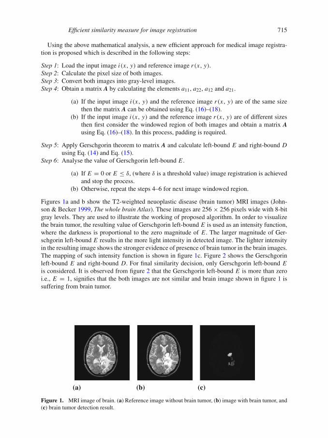
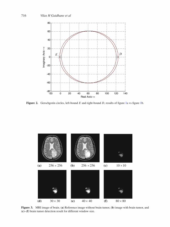
Figures 1a and b show the T2-weighted neuoplastic disease (brain tumor) MRI images (John-son & Becker 1999, The whole brain Atlas). These images are 256 × 256 pixels wide with 8-bitgray levels. They are used to illustrate the working of proposed algorithm. In order to visualizethe brain tumor, the resulting value of Gerschgorin left-bound E is used as an intensity function,where the darkness is proportional to the zero magnitude of E . The larger magnitude of Ger-schgorin left-bound E results in the more light intensity in detected image. The lighter intensityin the resulting image shows the stronger evidence of presence of brain tumor in the brain images.The mapping of such intensity function is shown in figure 1c. Figure 2 shows the Gerschgorinleft-bound E and right-bound D. For final similarity decision, only Gerschgorin left-bound Eis considered. It is observed from figure 2 that the Gerschgorin left-bound E is more than zeroi.e., E = 1, signifies that the both images are not similar and brain image shown in figure 1 issuffering from brain tumor.

(a) (b) (c)

Figure 1. MRI image of brain. (a) Reference image without brain tumor, (b) image with brain tumor, and(c) brain tumor detection result.


-20 0 20 40 60 80 100 120 140-80

-60

-40

-20

0

20

40

60

80

Real Axis-->

Imag

inar

y A

xis-

-->

E D

Figure 2. Gerschgorin circles, left-bound E and right-bound D, results of figure 1a vs figure 1b.

(a) 256256 (b) 256256 (c) 1010

(d) 3030 (e) 4040 (f) 8080

Figure 3. MRI image of brain. (a) Reference image without brain tumor, (b) image with brain tumor, and(c)–(f) brain tumor detection result for different window size.


5. Experimental results and discussions

In this section, the experimental results for evaluating the efficiency of the proposed similaritymeasure are presented. In this experiment, our focus is on the use of proposed similarity measuretechnique for image matching and hence the image registration.

Test samples shown in figure 3 are used to evaluate the effect of window size consideredfor the image registration. Figure 3a shows the reference image and figure 3b defective image(Glioma TITc-SPECT) (Johnson & Becker 1999, The whole brain Atlas) of 256 × 256 pixelswith 8-bit gray levels. Figures 3c–f show the detection results of defective area in the image for10 × 10, 30 × 30, 40 × 40 and 80 × 80 pixels window, respectively. The mapping of defectivearea shows that the small window of 10 × 10 pixels generates the noise in the detected imageand, therefore less visible to eyes. On other hand, a window size of 80 × 80 pixels results intothe false detection and increases the computational complexity due to the large size. Therefore,for best detection results and computational efficacy, medium window size in the range 30 to 40pixels size is preferred.

In the next experiment, the different sizes of neighbourhood windows are used in the pres-ence of different local distortion such as illuminations, noise and Point Spread Function (PSFs)effect to evaluate the efficiency of proposed similarity measure technique. Figure 4 shows the

Row1

Row2

Row3

Row4

Row5

(a) (b) (c) (d) (e)

-0.02 0 0.02 0.04 0.06-0.02

0

0.02

Real Axis-->

Imag

inar

y A

xis-

-->

E

0200

400

0200

400-0.5

0

0.5

X AxisY axis

Bou

nd E

-0.02 0 0.02 0.04 0.06-0.02

0

0.02

Real Axis-->

Ima

gin

ary

Axi

s---

>

E

0200

400

0200

400-0.5

0

0.5

X AxisY Axis

Bou

nd E

0 0.02 0.04 0.06-0.02

0

0.02

Real Axis-->

Imag

inar

y A

xis-

-->

E

0200

400

0200

400-0.5

0

0.5

X AxisY Axis

Bou

nd

E

0 0.05 0.1-0.02

0

0.02

Real Axis-->

Ima

gin

ary

Axi

s---

>

E

0200

400

0200

400-0.5

0

0.5

X AxisY Axis

Bo

un

d E

0 0.02 0.04 0.06-0.04

-0.02

0

0.02

0.04

Real Axis-->

Ima

gin

ary

Axi

s---

>

E

0200

400

0200

400-1

0

1

X AxisY Axis

Bou

nd

E

Figure 4. Image registration results of different window size template. (a) Reference image, (b) templateimage, (c) registration results, (d) Gerschgorin left-bound and circles, and (e) x , y coordinates for registeredposition.


Table 1. Gerschgorin left-bound E .

Figure Template size Maximum value of E

Figures 1a and b 256 × 256 1.009Figures 3a and b 10 × 10 5.757Figures 3a and b 30 × 30 4.755Figures 3a and b 40 × 40 4.555Figures 3a and b 80 × 80 5.054

image registration results using different template window size in the presence of different con-ditions. Here, all images are taken from standard brain image dataset and the template imagesare obtained from the reference image by cropping the defective area using Adobe Photoshop7.0.1 software.

In figure 4, row 1 shows the registration results for the image having the subacute strokedisease. The template image shows the particular affected region. In this experiment, the illu-mination (local distortion) effect having the brighten factor β = −0.7 is added in the referenceimage. The template of size 40 × 40 pixels matched with the illuminated image using proposedapproach. The Gerschgorin left-bound is closer to zero value (E = 0.0049). Thus, the pro-posed approach gives the best image registration result in the presence of different illuminationconditions.

Similarly, row 2 shows the registration results for the image with chronic subdural hematomadisease. The template of size 60 × 60 pixels is registered with the brighten image (β = 0.7). Inthis case, the Gerschgorin left-bound E = 0.0081, which is nearer to zero. In row 3, the resultsare shown for the image having the brain tumor. The tumor area is shown by the template imageof size 30 × 30 pixels. The reference image is now convolved with the Gaussian noise effect(variance v = 0.01). In this, the value of Gerschgorin left-bound is E = 0.0012. Row 4 showsthe registration results for Pick’s disease image. The reference image is convolved with salt-and-peppers noise (d = 0.02) and registered with the template image of size 50 × 50 pixels.In this case, the value of Gerschgorin left-bound is E = 0.0064. In row 5, an AIDS dementiadisease image is considered as reference image. The template image of the size 45 × 45 pixelsis registered with the reference image which is convolved with the point spread function (PSF)effect of h = 8 × 8 window. In this case, the Gerschgorin left-bound is also nearer to zero (E =0.0025). In these experiments, the different reference images with different illuminations, noises

Table 2. Comparison of normalized cross-correlation, eigenvalue-based similarity measure and proposedGerschgorin left-bound E with recovered x , y co-ordinates.

Normalized cross- Eigenvalue-based Gerschgorin-leftcorrelation (1 − μ) measure (λS) bound E

Template x , y (Andronache (Tsai & Yang (ProposedFigure 4 size co-ordinates et al 2008) 2005) method)

Row 1 40 × 40 (115, 175) 0.1049 0.1494 0.0049Row 2 60 × 60 (130, 100) 0.1281 0.3281 0.0081Row 3 30 × 30 (155, 130) 0.1110 0.1282 0.0012Row 4 50 × 50 (115, 100) 0.1462 0.4181 0.0064Row 5 45 × 45 (115, 110) 0.1378 0.2120 0.0025


(a) (b) (c)

(d) (e) (f)

Figure 5. Brain tumor detection. (a) Reference image without brain tumor, (b) template image withGaussian noise, (c)–(f) images with growing brain tumor.

and PSF effects are considered. In all cases, the similarity measure Gerschgorin left-bound iscloser to zero, whereas the value of normalized cross-correlation and eigenvalue-based similaritymeasure are larger which further results into dissimilarity result. Thus, the proposed approachoutperforms in the presence of different illumination, noise and PSF conditions.

Table 1 shows Gerschgorin left-bound for different windowed template images. The value ofGerschgorin left-bound E should be larger for dissimilar images.

Table 2 shows the recovered x and y coordinates position of different windowed templateimages in the reference images. It also shows the comparison of normalized cross-correlation,eigenvalue-based similarity measure and proposed Gerschgorin left-bound E . For the perfecttemplate matching, the value of 1−μ, λS and Gerschgorin left-bound E should be zero or nearerto zero.

From table 2, it is observed that the value of normalized cross-correlation and smallesteigenvalue-based similarity measure is greater than Gerschgorin left-bound E which may result

Table 3. Comparison of normalized cross-correlation, eigenvalue-based similaritymeasure and proposed Gerschgorin left-bound E for growing brain tumor detection.

Normalized cross- Eigenvalue-based Gerschgorin left-bound EFigures correlation (1 − μ) measure (λS) (Proposed approach)

Figure 5a vs b 0.426 0.612 0.257Figure 5a vs c 0.259 0.408 0.478Figure 5a vs d 0.317 0.637 0.832Figure 5a vs e 0.426 0.841 1.143Figure 5a vs f 0.709 1.275 2.117


Table 4. Comparison of computational time and computational complexity of the normalizedcross-correlation, eigenvalue-based and proposed approach.

Computational time Computational Time savedSimilarity measure methods (seconds) complexity (seconds)

Normalized cross-correlation (μ) 0.3954 (255)3 + (255)2 –Eigenvalue-based method (λS) 0.3618 (255)3 + (4)3 0.0336Proposed approach (E) 0.2239 (255)2 + (4) 0.1715

into false similarity decision. This is due to the fact that the smaller eigenvalue is more affectedby the noises or local disturbances.

Further, we perform the experiments to evaluate the effect of minor variations in the braintumor size on the threshold value δ as well as the final similarity decision. In this analysis, aT2-weighted (MR-T2) healthy brain image is considered as a reference image which is shownin figure 5a and, figure 5b shows the noisy (Gaussian noise) test image without brain tumor.Similarly, the gradual growth of tumor is shown in figures 5c–f. In these experiments, braintumor detection test is performed using different existing techniques as well as using proposedmethod. The selection of threshold value plays an important role in the final tumor detectiondecision. If we consider the threshold value as δ = 0.3, then a tumor is said to be detectedonly when the similarity measure value is greater than this threshold value, i.e., δ = 0.3. Now,we first consider the effect of noise on the final similarity decision. For this experiment, weconsider figure 5a as a reference image and figure 5b as the noisy tumor-less test image. Thevarious values of normalized cross-correlation (1 − μ), eigenvalue-based similarity measure(λS) and Gerschgorin left-bound (E) are shown in first row of table 3. From this first row, it isobserved that the value of normalized cross-correlation is 0.426 and eigenvalue-based similaritymeasure is 0.612 which is greater than the threshold value i.e., δ = 0.3. These higher valuesshow that the tumor is detected in the brain. However, it is a false decision since figure 5b iswithout tumor. Using proposed approach, the value of Gerschgorin left-bound E is 0.257 whichis less than the threshold value and hence shows the tumor-less decision. From this experiment,it is proved that the proposed method is more accurate for small variations in local noise anddisturbances. Further, this test for brain tumor detection is also performed for different tumors.For this experiments, the reference image, figure 5a is compared with the gradually growingbrain tumor images, as shown in figures 5c–f. Similar to above experiments on tumor detection,the various similarity measures are obtained which are shown from rows 2 to 4 in table 3. Thevalue of similarity measures should be larger than the threshold value for correct tumor detectiondecision. From these rows in table 3, it is observed that the proposed Gerschgorin left-bound Eis greater than the threshold value as well as the normalized cross-correlation and eigenvalue-based similarity measure. This larger value of Gerschgorin bound E shows the strong evidenceof the brain tumor and avoids the confusion in final tumor detection decision. Thus, the proposedmethod is more accurate and promising good results.

All experiments are carried out on an Intel(R) Core(TM) i3 CPU with 2.4 GHZ frequencyand 4 GB RAM. The similarity measures are tested on the matrix laboratory (MATLAB) plat-form of version 7.0.4. Table 4 shows the comparison of computational time required by variousimage registration methods. Figures 5a and c of the size 256 × 256 pixels are considered for thecalculation of computational time of various similarity measures. Moreover, the computationalcomplexity and time saving is also summarized in table 4.


6. Conclusion

In this paper, an efficient similarity measure approach is proposed for medical image registra-tion which is based on the Gerschgorin circles theorem. The value of Gerschgorin left-boundis ideally zero for identical images and large value (more than threshold value) for dissimilarimages. Experimental results have shown that the proposed similarity measure approach is supe-rior and computationally efficient in comparison to the traditional similarity measures. Moreover,it is highly sensitive to the small defective area diagnosis and tolerable to illumination changes,noise and PSFs. This method can be useful in other medical imaging applications such asimage recognition, defects detection MRI, CT scan, mismatching between fMRI and EEG/MEGimages etc.

References

Andronache A, Siebenthal M V, Székely G and Cattin Ph 2008 Non-rigid registration of multi modal imagesusing both mutual information and cross-correlation. Med. Image Anal. 12: 3–15

Gaidahne V H, Hote Y V and Singh V 2012 Nonrigid image registration using efficient similarity measureand Levenberg-Marquardt optimization. Biomed. Eng. Lett. 2: 118–123

Gerschgorin S 1931 Ueber die abgrenzung der eigenwerte einer matrix. Izv. Akad Nauk SSSR Ser. Mat. 1:749–754

Hote Y V 2009 New approach of Kharitonov and Gerschgorin theorem in control system. Submitted toDelhi University

Hote Y V, Choudhury D R and Gupta J R P 2006 Gerschgorin theorem and its applications in controlsystem problems. Proc. IEEE international conference on industrial technology 2438–2443

Hote Y V, Gupta J R P and Choudhury D R 2011 A simple approach for stability margin of discrete systems.J. Control Theory Applicat. 9: 567–570

Johnson K A and Becker J A 1999 The Whole Brain Atlas, Harvard Medical School, http://www.med.harvard.edu/aanlib

Jung Y-J and Im C-H 2011 An improved technique to consider mismatch between fMRI and EEG/MEGsources for fMRI constrained EEG/MEG source imaging. Biomed. Eng. Lett. 1: 32–41

Lindoso A and Entrena L 2007 High performance FPGA-based image correlation. J. Real-Time ImageProcess. 2: 223–233

Lu X, Zhang S, Su H and Chen Y 2008 Mutual information-based multimodal image registration using anovel joint histogram estimation. Comput. Med. Imaging Graphics 32: 202–209

Pan W, Qin K and Chen Y 2009 An adaptable-multilayer fractional Fourier transform approach for imageregistration. IEEE Trans. Pattern Anal. Mach. Intell. 31: 400–413

Sun T-H, Liu C-S and Tien F-C 2008 Invariant 2D object recognition using eigenvalues of covariancematrices, re-sampling and autocorrelation. Expert Syst. Appl. 35: 1966–1977

Tsai D-M and Yang R-H 2005 An eigenvalue-based similarity measure and its application in defectdetection. Image Vision Comput. 23: 1094–1101

Viola P and Wells W M 1997 Alignment by maximization of mutual information. Int. J. Comput. Vision24: 137–154

Zheng D, Zhao J and Saddik A E 2003 RST-invariant digital image watermarking based on log-polarmapping and phase correlation. IEEE Trans. Circuits Syst. Video Technol. 13: 753–765

Zitová B and Flusser J 2003 Image registration methods: a survey. Image Vision Comput. 21: 977–1000

http://www.med.harvard.edu/aanlib

http://www.med.harvard.edu/aanlib

an efficient similarity measure technique for medical image

Documents