an empirical analysis of earnings and employment...
TRANSCRIPT
An Empirical Analysis of Earnings and Employment Risk
Luigi Guiso Ente Luigi Einaudi
Via Due Macelli 73, 00187 Rome, Italy, email: [email protected]
Tullio Jappelli CSEF, Department of Economics, Università di Salerno
84084 Fisciano (Salerno), Italy, email: [email protected]
Luigi Pistaferri Department of Economics, Stanford University,
Stanford, CA 94305-6072, USA, email: [email protected]
Forthcoming in the Journal of Business and Economic Statstistics
1
Abstract The mean and higher moments of the distribution of future income are crucial determinants of individual choices. These moments are usually estimated in panel data from past income realizations. In this paper we rely instead on subjective expectations available in the 1995 Survey of Household Income and Wealth, a large random sample representative of Italian households. The survey elicits information on the distribution of future earnings and on the probability of unemployment. Analysis of this distribution helps us understanding how individual uncertainty evolves over the life cycle and if attitudes towards risk affect occupational choices and income riskiness. Key words: Subjective expectations, income risk, unemployment. JEL classification: E21.
2
1. INTRODUCTION
Economists routinely propose models in which current decisions depend on expectations
of future variables. For instance, theories of intertemporal choice with incomplete markets posit
that people react to expected income. When the strong assumptions that lead to certainty
equivalence are relaxed, theory also predicts that people respond to higher moments of the
distribution of future income (Kimball 1990). The relevant moments are those of the subjective
income distribution conditional on information available at the time the decisions are made.
Only under the extreme hypothesis of complete markets the measurement of individual
income risk is not an issue. But when idiosyncratic shocks matter, measuring microeconomic
uncertainty becomes a crucial issue in applied econometrics and in calibration of general and
partial equilibrium models. In a recent survey, Browning, Hansen and Heckman (1999) argue that
calibrating economic models with imperfect insurance “requires a measure of the magnitude of
microeconomic uncertainty, and how that uncertainty evolves over the business cycle [...]. This
introduces the possibility of additional sources of heterogeneity because different economic
agents may confront fundamentally different risks”.
These remarks have implications for many areas of research. Measuring individual
uncertainty is crucial when trying to determine the importance of precautionary saving. Individual
uncertainty affects the width of the inaction band in Ss models of durable demand and housing
investment. Income risk can lead prudent individuals to demand a higher risk premium on risky
assets, affects portfolio choice and the demand for insurance against insurable risks. More
generally, income risk can impact labor supply, education and occupation choice, job search, and
many other economic decisions.
Two approaches have emerged in the literature to extract moments of the distribution of
future income from observable variables. One relies on panel data and infers expectations and
possibly higher moments of the individual distribution from past income realizations. To be
valid, this method requires assuming that individuals condition on the same set of variables to
form expectations, that the individuals and the econometrician have the same information set and
that the econometrician knows the stochastic process that generates individual expectations. It is
3
an unhappy feature of applied economics that implausible assumptions and procedures get
accepted for lack of sound alternatives.
A second strand of literature has recently proposed to rely on survey questions, not
retrospective data, to elicit information on the conditional distribution of future income. The
main advantage of survey questions over inference based on realizations is that they do not
require the econometrician to know the variables that individuals consider in forming their
expectations.
Following this line of research, we rely on subjective expectations drawn from the 1995
Survey a Household Income and Wealth (SHIW), a large representative sample of the Italian
population. As will be seen, to estimate the moments of the income distribution from survey data
we must rely on some assumptions and imputations specific to our dataset.
Our contribution to the literature is on method and substance. On the methodological side,
we take explicitly into account that the distribution of future income results from three distinct
elements: the probability of job loss, the distribution of future wages and the distribution of
unemployment compensation. Depending on the institutional features of the labor market, each
of these elements may be more or less important in determining the overall income distribution.
For instance, if job search is costless and wages and prices are fully flexible, future income
depends only on wage fluctuations; but if wages are sticky or fixed, income variability depends
mainly on fluctuations in employment status. Previous studies focus mainly on wages or income
from all sources. The distribution of wages neglects the impact of the probability of
unemployment and the distribution of benefits. Expectations about income from all sources make
it hard (if not impossible) to assess the separate impact of wage and unemployment uncertainty
on overall income uncertainty. Subjective information on future employment prospects available
in the 1998 SHIW allows us to tackle the first issue directly. Moreover, we can use external
information to impute unemployment benefits as a function of various demographic and labor
status variables, thus accounting for the second element.
On substance, we provide evidence that is useful for various branches of research that,
directly or indirectly, need to make assumptions about various moments of the conditional
distribution of individual incomes. First, we construct empirical profiles of income uncertainty
4
and of the probability of unemployment over the working career. The estimated age profiles help
us understanding how uncertainty evolves over the life cycle. The analysis is important because
simulation studies always neglect age-related heterogeneity in income risk. Second, we compare
unemployment risk in Italy and in the US using comparable survey questions. This allows us to
highlight the role of labor market flexibility and other institutional factors. Finally, we relate
unemployment risk, the coefficient of variation of future income and an index of the asymmetry
of the income distribution to a set of demographic characteristics and to an index of risk aversion.
The correlation between income risk and risk aversion allows us to assess the severity of the self-
selection problem that potentially plagues many empirical studies of precautionary saving and
portfolio choice. The relation between our measures of earnings uncertainty and workers’
characteristics helps identifying variables associated with job security.
The rest of the paper is organized as follows. In Section 2 we survey the literature based
on subjective income expectations and describe the main characteristics of the survey. In Section
3 we estimate the overall individual labor income distribution combining the probability of
unemployment with information on future earnings and imputation of unemployment benefits. In
Section 4 we provide ample description of the cross-sectional characteristics of the income
distributions. In Section 5 we present the age profiles of the probability of unemployment and of
the coefficient of variation of future income. The cross-country comparison between
unemployment risk in Italy and the United States is taken up in Section 6. In Section 7 we test if
individuals that face lower income risk also are more risk-averse. Section 8 summarizes our main
findings.
2. PREVIOUS EVIDENCE AND SAMPLE DESIGN
In order to derive empirical measures of subjective income expectations and income risk,
one must design appropriate survey questions to characterize either the density or the cumulative
distribution function of future income. In the literature both approaches have been taken. Guiso,
Jappelli and Terlizzese (1992) is based on survey questions posed in the 1989 SHIW eliciting
5
information about the density of future earnings. Recently, Dominitz and Manski (1997a, b),
Dominitz (1998), and Das and Donkers (1999) have followed the alternative approach; so does
the design of the 1995 SHIW.
The 1995 SHIW has data on income, consumption, financial wealth, real estate wealth,
and several demographic variables for a representative sample of 8,135 Italian households (see
Appendix A). A special section of the survey was designed to characterize the distribution of
future income and the probability of unemployment. To our knowledge, the only two other
surveys containing information on employment prospects are the Health and Retirement Survey
(HRS), conducted at the University of Michigan since 1992, and the Survey of Economic
Expectations (SEE), conducted at the University of Wisconsin-Madison since 1994. The SEE is a
national telephone survey of the US population. The survey is limited in scope and small in size
(1,300 households interviewed in 1996). The drawbacks of the HRS data are that the survey has
no questions about income expectations and that respondents’ age is deliberately restricted to the
51-61 range (in 1992), i.e. individuals approaching retirement for whom unemployment risk
could be negligible or altogether absent. Explicitly considering unemployment probabilities at
younger ages is important, because employment risk is one of the major determinants of future
income prospects.
Our survey questions focus on earnings rather than disposable income and on individuals
rather than households. Focus on earnings avoids mixing labor income and capital income
uncertainty. Focus on individuals avoids relying on one person to evaluate the income prospects
of other household members. Unlike the SEE, the 1995 SHIW households report the distribution
of after-tax income, rather than gross income. One advantage of using after-tax income is that
most household choices ultimately depend on disposable income, not income before taxes.
Furthermore, since in Italy income taxes and social security contributions are withheld at source,
employees are better informed about their after-tax earnings.
Questions on income expectations were asked to half of the overall sample after excluding
the currently retired and people not in the labor force (a total of 4,799 individuals, randomly
chosen among about 10,000 survey participants). Both the employed, the unemployed and the job
seekers are asked to state, on a scale from 0 to 100, their chances of having a job in the 12 months

6
following the interview. Each individual assigning a positive probability to being employed is
then asked to report the minimum (ym) and the maximum (yM) incomes he or she expects to earn
if employed, and the probability of earning less than the midpoint of the support of the
distribution, Prob(y ≤ (ym+ yM)/2) = π. The wording of these questions is reported in Appendix B.
The employment probability question aims at obtaining this probability for both the
currently employed and the unemployed, taking into account job mobility, i.e., that some
respondents plan to quit or to change job. However, in practice the interpretation of the question
could be different for the currently employed and for the unemployed. Moreover, it is not clear
that the respondent, if employed, reports only involuntary job losses rather than any change in
employment status (including job mobility). Thus, the question could be subject to measurement
error and misrepresent true unemployment risk. In Section 4 we will therefore cross-examine the
reliability of the unemployment question by comparing the average subjective unemployment
probability with actual unemployment rates drawn from labor force statistics; we also compare
unemployment probabilities with actual labor market transition probabilities.
In the next section we describe how we combine the information derived from the survey
questions to estimate the distribution of future income, both conditional and unconditional on
working. From the original 4,799 observations, we exclude 209 who expected to retire or to drop
out from the labor force within a year and 385 individuals with missing data on the relevant
questions. The non-response rate is therefore 8 percent (385/4590), and the final sample includes
4,205 individuals.
3. THE INDIVIDUAL DISTRIBUTIONS
The distribution of future income depends on the distribution of future earnings if the
individual is employed and on the distribution of unemployment benefits if he or she is
unemployed. The two distributions have to be weighted by the probability of the two states, so
that the distribution of future income is the mixture of two distributions:
7
−=
ii
ii
i
pb
pyx
yprobabilitwith
)1(yprobabilitwith (1)
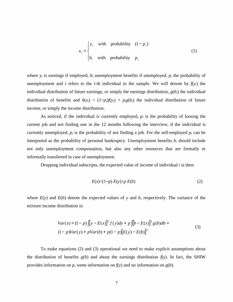
where yi is earnings if employed, bi unemployment benefits if unemployed, pi the probability of
unemployment and i refers to the i-th individual in the sample. We will denote by f(yi) the
individual distribution of future earnings, or simply the earnings distribution, g(bi) the individual
distribution of benefits and h(xi) = (1−pi)f(yi) + pig(bi) the individual distribution of future
income, or simply the income distribution.
As noticed, if the individual is currently employed, pi is the probability of loosing the
current job and not finding one in the 12 months following the interview; if the individual is
currently unemployed, pi is the probability of not finding a job. For the self-employed pi can be
interpreted as the probability of personal bankruptcy. Unemployment benefits bi should include
not only unemployment compensation, but also any other resources that are formally or
informally transferred in case of unemployment.
Dropping individual subscripts, the expected value of income of individual i is then:
E(x)=(1−p) E(y)+p E(b) (2)
where E(y) and E(b) denote the expected values of y and b, respectively. The variance of the
mixture income distribution is:
[ ] [ ][ ]2
22
)()()1()()()1(
)()()()()1()(
bEyEppbpVaryVarp
dbbgxEbpdyyfxEypxVar
−−++−
=−+−−= ∫∫ (3)
To make equations (2) and (3) operational we need to make explicit assumptions about
the distribution of benefits g(b) and about the earnings distribution f(y). In fact, the SHIW
provides information on p, some information on f(y) and no information on g(b).
8
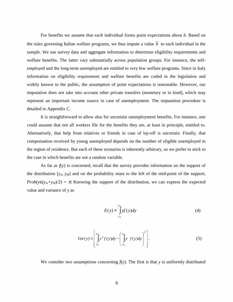
For benefits we assume that each individual forms point expectations about b. Based on
the rules governing Italian welfare programs, we thus impute a value b to each individual in the
sample. We use survey data and aggregate information to determine eligibility requirements and
welfare benefits. The latter vary substantially across population groups. For instance, the self-
employed and the long-term unemployed are entitled to very few welfare programs. Since in Italy
information on eligibility requirement and welfare benefits are coded in the legislation and
widely known to the public, the assumption of point expectations is reasonable. However, our
imputation does not take into account other private transfers (monetary or in kind), which may
represent an important income source in case of unemployment. The imputation procedure is
detailed in Appendix C.
It is straightforward to allow also for uncertain unemployment benefits. For instance, one
could assume that not all workers file for the benefits they are, at least in principle, entitled to.
Alternatively, that help from relatives or friends in case of lay-off is uncertain. Finally, that
compensation received by young unemployed depends on the number of eligible unemployed in
the region of residence. But each of these scenarios is inherently arbitrary, so we prefer to stick to
the case in which benefits are not a random variable.
As far as f(y) is concerned, recall that the survey provides information on the support of
the distribution [ym, yM] and on the probability mass to the left of the mid-point of the support,
Prob(y≤(ym+yM)/2) = π. Knowing the support of the distribution, we can express the expected
value and variance of y as
∫=M
m
y
y
dyyyfyE )()( (4)
−= ∫∫
2
2 )()()(M
m
M
m
y
y
y
y
dyyfydyyfyyVar . (5)
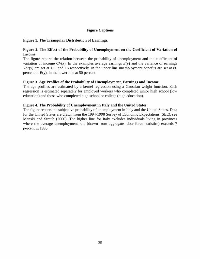
We consider two assumptions concerning f(y). The first is that y is uniformly distributed
9
over each of the two intervals [ym, (ym+yM)/2] and ((ym+yM)/2, yM]. If π=0.5 the distribution
collapses to a single uniform distribution defined in the [ym, yM] interval. A second possibility is
to assume that the distribution is triangular over the same two intervals; if π=0.5 the distribution
again collapses to a single triangular distribution over the [ym, yM] interval. The expressions to
compute the mean and the variance of the triangular distributions are reported in Appendix D.
Note that in both cases E(y) and Var(y) depend only on the three known parameters, ym , y M , and
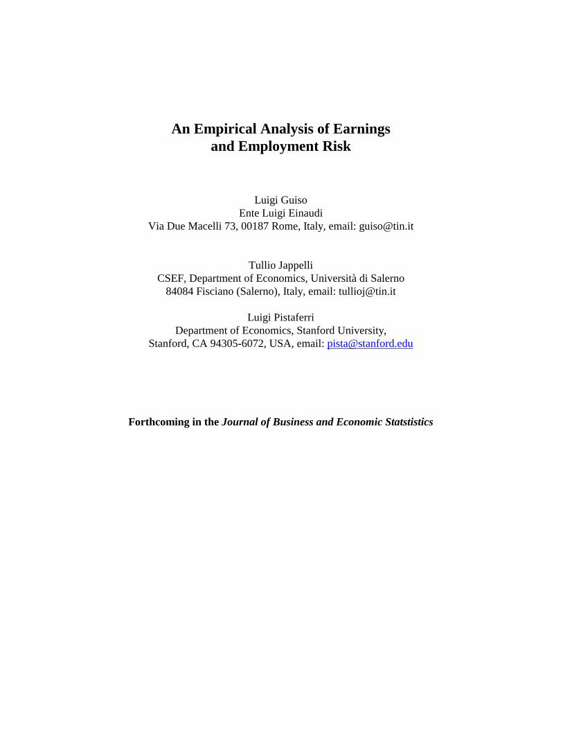
π. The triangular distribution (shown in Figure 1) is a more plausible description of the
probability distribution of earnings, because outcomes further away from the mid-point receive
less weight. For this reason in the remainder of the paper we report statistics computed according
to the triangular distribution. We also checked the sensitivity of the results on the assumption of a
uniform distribution. All results were very similar and are not reported for brevity.
If people have point expectations about benefits, Var(b)=0 and we can rewrite equations
(2) and (3) as:
bpyEpxE +−= )()1()( (6)
[ ]2)()1()()1()( byEppyVarpxVar −−+−= (7)
The coefficient of variation provides a convenient measure of income risk that is
particularly useful for comparison between different individuals, groups or samples. The
coefficient of variation of earnings, CV(y)=Sd(y)/E(y), is immediately obtained by the ratio
between the square root of equation (5) and equation (4). It is of course affected by distributional
assumptions. The coefficient of variation of income is:
[ ]bpyEp
byEppyVarpxExSdxCV
+−−−+−
==)()1(
)()1()()1()()()(
2
(8)
Equation (8) highlights that the relation between the probability of unemployment and overall
10
income risk, as measured by CV(x), is non-linear. The standard deviation of income Sd(x) equals
the standard deviation of earnings if p=0 and zero if p=1, is concave in p and is maximized when
( ) [ ]{ } 5.0*)(15.0 2 <=−−×= pbyEyVarp . Thus an increase in p above p* reduces expected
income and raises Sd(x). The probability p affects also the expectation of income (the
denominator of equation 8), so that the relation between p and CV(x) too is a non-linear function
of Var(y), E(y) and b .
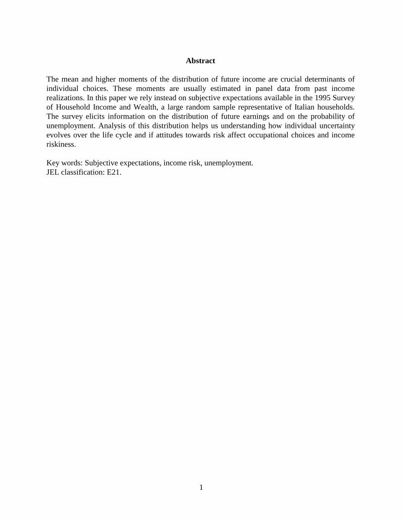
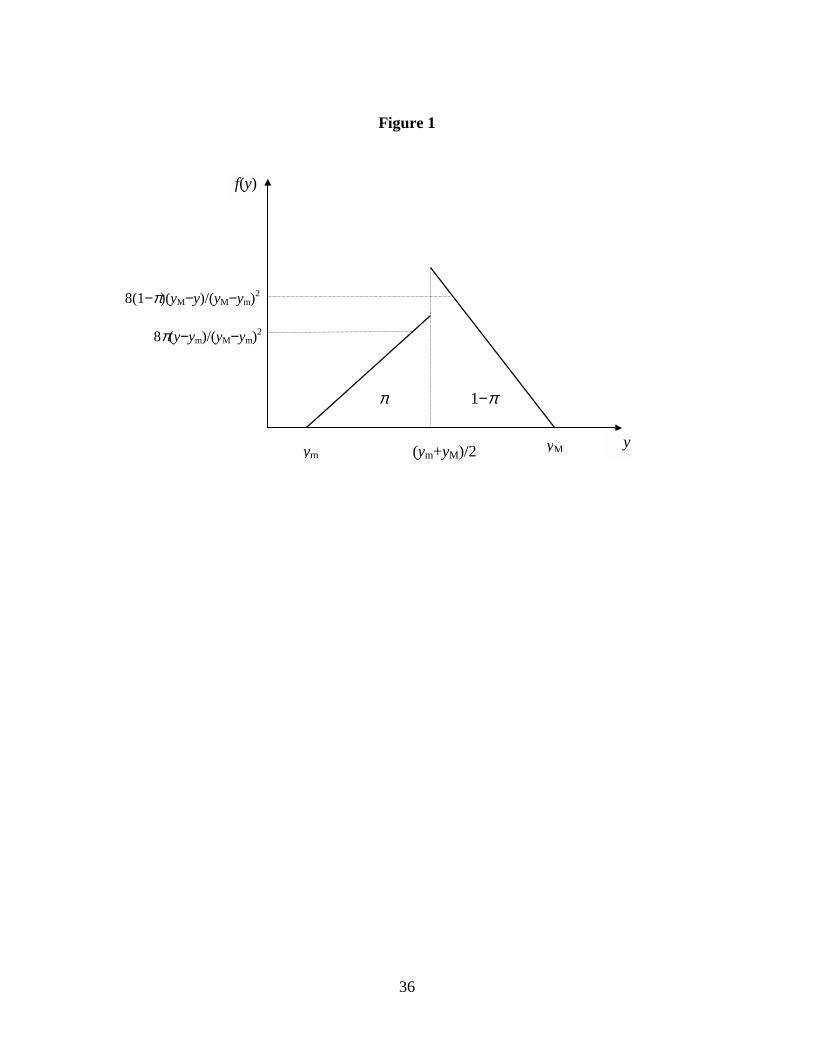
This is illustrated in Figure 2, where we set E(y)=100 and Var(y)=16, so that CV(y)=4
percent; as will be seen in Section 4, this value is close to the median coefficient of variation of
earnings in our sample. The figure reports CV(x) of individuals with the same earnings
distribution but different unemployment probabilities. The lower curve plots CV(x) as a function
of p if b =0.8×E(y), approximately the level of benefits large firm employees are entitled to. For
an individual with p=0.2 (about the sample average of the probability in our sample), CV(x) is 8
percent. The coefficient of variation reaches a maximum at 10 percent for an individual with
p=0.5, and then declines for individuals with higher values of p. The higher curve refers to
individuals who are entitled to b =0.50×E(y); as explained in Appendix C, this situation is typical
of small firm employees. The much larger value of [E(y)−b ] raises the weight of p in
determining the riskiness of future income. For an individual with p=0.2, CV(x) is now 22
percent. The impact of the probability of unemployment is maximum for an individual with p=70
percent, CV(x)=35 percent.
Figure 2 shows that CV(x) is very sensitive to the level of unemployment benefits at all
levels of p. The imputation of b can be questionable, particularly because it neglects informal
transfers. Thus in the next section we report information on both CV(y), which is independent
from b and p, and on CV(x).
Since we have an estimate of the distributions at the individual level, we can easily check
if the distributions are symmetric. We thus construct and analyze an index of skewness of the
distributions, [ ] )(/)()()( ySdyEyMyAS −= for earnings and [ ] )(/)()()( xSdxExMxAS −= for
income, where )(⋅M is the median of the distribution. The formula for the median is reported in
Appendix D. In Section 7 we will consider more in detail how this index varies with individual
11
characteristics.
4. THE CROSS-SECTIONAL DISTRIBUTIONS
The foregoing definitions and assumptions allow us to compute the mean and variance of
both future earnings and future income for each individual in the sample, and therefore to obtain
a cross-sectional distribution of individual means and variances. These cross-sectional
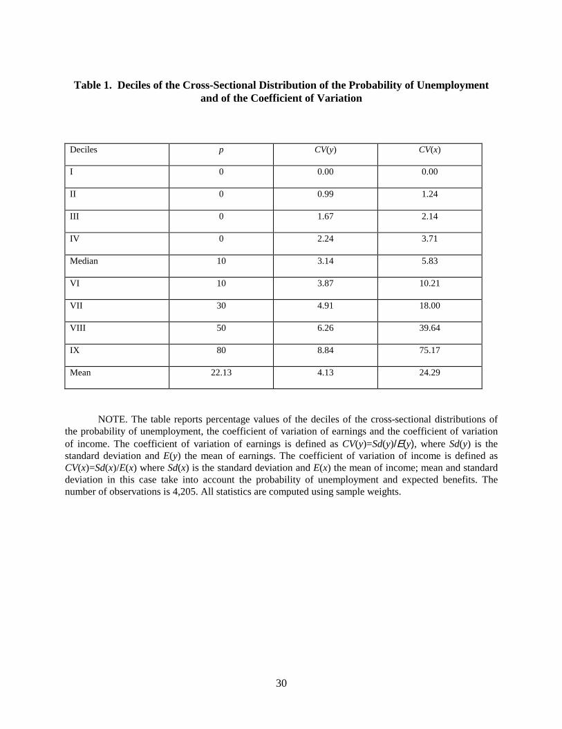
distributions are conveniently summarized in Table 1 by the cross-sectional distribution of the
probability of unemployment and of the individual coefficient of variation.
Column (1) of Table 1 displays the cross-sectional distribution of p. For over 40 percent
of the sample p=0, a signal of substantial rigidity in the labor market; the incidence of p=0 among
the employed is even higher. On the other hand, only 3 percent of the sample is certain to be
unemployed in the year following the interview (p=1). A sizable fraction of the sample reports
substantial unemployment uncertainty: for 20 percent the probability exceeds 50 percent. As we
argue in Section 2, due to the wording of the questions, for some individuals a high p does not
necessarily reflect worsening employment prospects. For instance, women who anticipate having
a child, or young men expecting compulsory military service may correctly report temporary exit
from the labor force in the year following the survey, rather than job dismissal or inability to find
a job.
Columns (2) displays the deciles of the coefficient of variation of earnings,
CV(y)=Sd(y)/E(y). The cross-sectional distribution of the coefficient of variation CV(y) is right
skewed, as shown by the positive difference between the cross-sectional mean, equal to 4.13
percent, and the cross-sectional median, 3.14 percent.
The cross-sectional distribution of CV(y) can be compared with previous evidence for
Italy. Guiso et al. (1992) use subjective expectations from the 1989 SHIW. Since no question on
employment prospects was asked in 1989, a proper comparison between the 1995 and the 1989
SHIW must focus on CV(y). In that survey respondents were asked a rather different set of
questions about earnings prospects. They had to assign probability weights, summing to 100, to a
12
set of intervals of income changes over the 12 months following the interview.
It is not obvious whether asking questions about the density function of future income is
more effective (in terms of minimizing the probability of non-response and in eliciting
meaningful data) than questions about the cumulative distribution function. We can provide some
evidence on this important issue comparing non-responses to the questions on expectations in the
1989 and 1995 SHIW. In 1989 5,954 of those interviewed did not answer the questions on the
subjective income density function (a non-response rate of 43 percent). In 1995 the fraction of
non-respondents to the questions on the cumulative distribution was only 8 percent. In contrast,
in 1989 a much higher faction of respondents reported no income risk (34 percent), while the
same fraction in 1995 was only 13 percent. The much higher response rate suggests that the 1995
questions concerning the cumulative distribution function are easier to grasp and thus provide
more reliable information. Further evidence (not reported for brevity) indicates that the
probability of non-response in 1989 is statistically significantly lower for the more educated, the
resident in the North and the young. In contrast, the same demographic variables do not
significantly affect the probability of non-response in 1995.
Regardless of the assumptions on the shape of the distribution, the cross-sectional average
of CV(y) is higher in 1995 than in 1989 (about 2 percent), reflecting differences in sample design
and risk across sample periods. In fact, the 1995 interviews were completed between May and
October of 1996 (a recession year), whereas the 1989 interviews were completed in the spring of
1990, at the end of an upswing. Nonetheless, CV(y) in both years is fundamentally characterized
by the small magnitude of income risk.
Column (3) of Table 1 reports the cross-sectional distribution of the coefficient of
variation of income, CV(x)=Sd(x)/E(x), which combines the variance of earnings with
information on the probability of unemployment and the imputation of benefits (see equation 8).
For the bottom part of the distribution, where p is near or exactly zero, there is not much
difference between CV(y) and CV(x). But already at the median the impact of p is substantial: the
cross-sectional median of CV(x) is 5.83 percent. In the top two deciles the impact of p and of
imputed benefits is dramatic, because the coefficient of variation exceeds 40 percent, so that the
overall cross-sectional mean is 24.29 percent. The high values in the top two deciles often refer
13
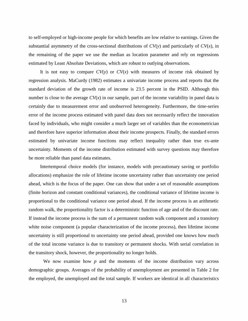
to self-employed or high-income people for which benefits are low relative to earnings. Given the
substantial asymmetry of the cross-sectional distributions of CV(y) and particularly of CV(x), in
the remaining of the paper we use the median as location parameter and rely on regressions
estimated by Least Absolute Deviations, which are robust to outlying observations.
It is not easy to compare CV(y) or CV(x) with measures of income risk obtained by
regression analysis. MaCurdy (1982) estimates a univariate income process and reports that the
standard deviation of the growth rate of income is 23.5 percent in the PSID. Although this
number is close to the average CV(x) in our sample, part of the income variability in panel data is
certainly due to measurement error and unobserved heterogeneity. Furthermore, the time-series
error of the income process estimated with panel data does not necessarily reflect the innovation
faced by individuals, who might consider a much larger set of variables than the econometrician
and therefore have superior information about their income prospects. Finally, the standard errors
estimated by univariate income functions may reflect inequality rather than true ex-ante
uncertainty. Moments of the income distribution estimated with survey questions may therefore
be more reliable than panel data estimates.
Intertemporal choice models (for instance, models with precautionary saving or portfolio
allocations) emphasize the role of lifetime income uncertainty rather than uncertainty one period
ahead, which is the focus of the paper. One can show that under a set of reasonable assumptions
(finite horizon and constant conditional variances), the conditional variance of lifetime income is
proportional to the conditional variance one period ahead. If the income process is an arithmetic
random walk, the proportionality factor is a deterministic function of age and of the discount rate.
If instead the income process is the sum of a permanent random walk component and a transitory
white noise component (a popular characterization of the income process), then lifetime income
uncertainty is still proportional to uncertainty one period ahead, provided one knows how much
of the total income variance is due to transitory or permanent shocks. With serial correlation in
the transitory shock, however, the proportionality no longer holds.
We now examine how p and the moments of the income distribution vary across
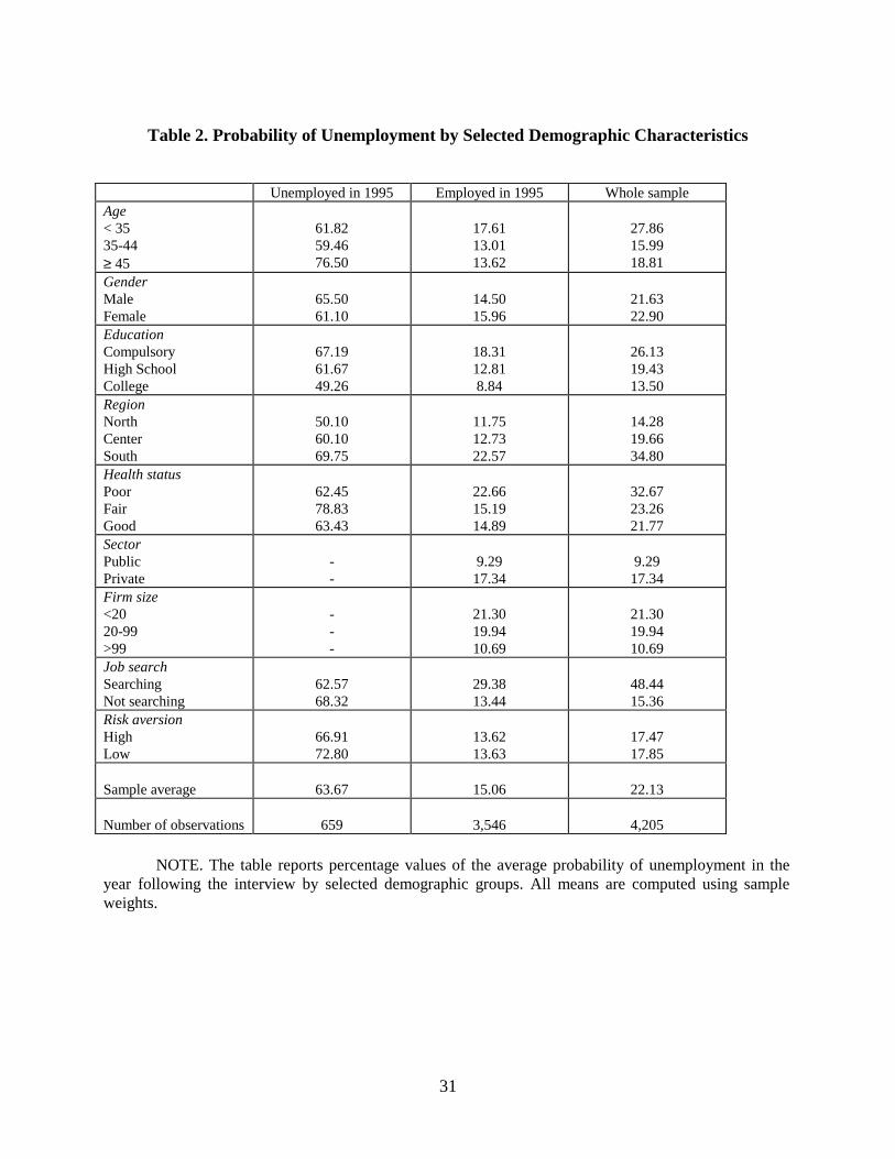
demographic groups. Averages of the probability of unemployment are presented in Table 2 for
the employed, the unemployed and the total sample. If workers are identical in all characteristics
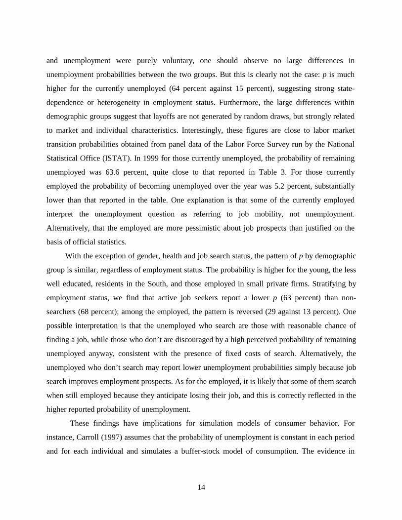
14
and unemployment were purely voluntary, one should observe no large differences in
unemployment probabilities between the two groups. But this is clearly not the case: p is much
higher for the currently unemployed (64 percent against 15 percent), suggesting strong state-
dependence or heterogeneity in employment status. Furthermore, the large differences within
demographic groups suggest that layoffs are not generated by random draws, but strongly related
to market and individual characteristics. Interestingly, these figures are close to labor market
transition probabilities obtained from panel data of the Labor Force Survey run by the National
Statistical Office (ISTAT). In 1999 for those currently unemployed, the probability of remaining
unemployed was 63.6 percent, quite close to that reported in Table 3. For those currently
employed the probability of becoming unemployed over the year was 5.2 percent, substantially
lower than that reported in the table. One explanation is that some of the currently employed
interpret the unemployment question as referring to job mobility, not unemployment.
Alternatively, that the employed are more pessimistic about job prospects than justified on the
basis of official statistics.
With the exception of gender, health and job search status, the pattern of p by demographic
group is similar, regardless of employment status. The probability is higher for the young, the less
well educated, residents in the South, and those employed in small private firms. Stratifying by
employment status, we find that active job seekers report a lower p (63 percent) than non-
searchers (68 percent); among the employed, the pattern is reversed (29 against 13 percent). One
possible interpretation is that the unemployed who search are those with reasonable chance of
finding a job, while those who don’t are discouraged by a high perceived probability of remaining
unemployed anyway, consistent with the presence of fixed costs of search. Alternatively, the
unemployed who don’t search may report lower unemployment probabilities simply because job
search improves employment prospects. As for the employed, it is likely that some of them search
when still employed because they anticipate losing their job, and this is correctly reflected in the
higher reported probability of unemployment.
These findings have implications for simulation models of consumer behavior. For
instance, Carroll (1997) assumes that the probability of unemployment is constant in each period
and for each individual and simulates a buffer-stock model of consumption. The evidence in
15
Table 2 is strongly at variance with this assumption.
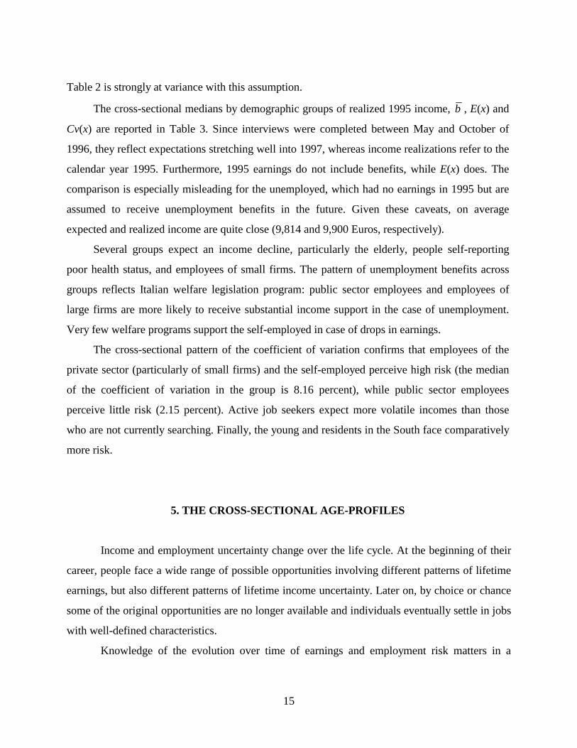
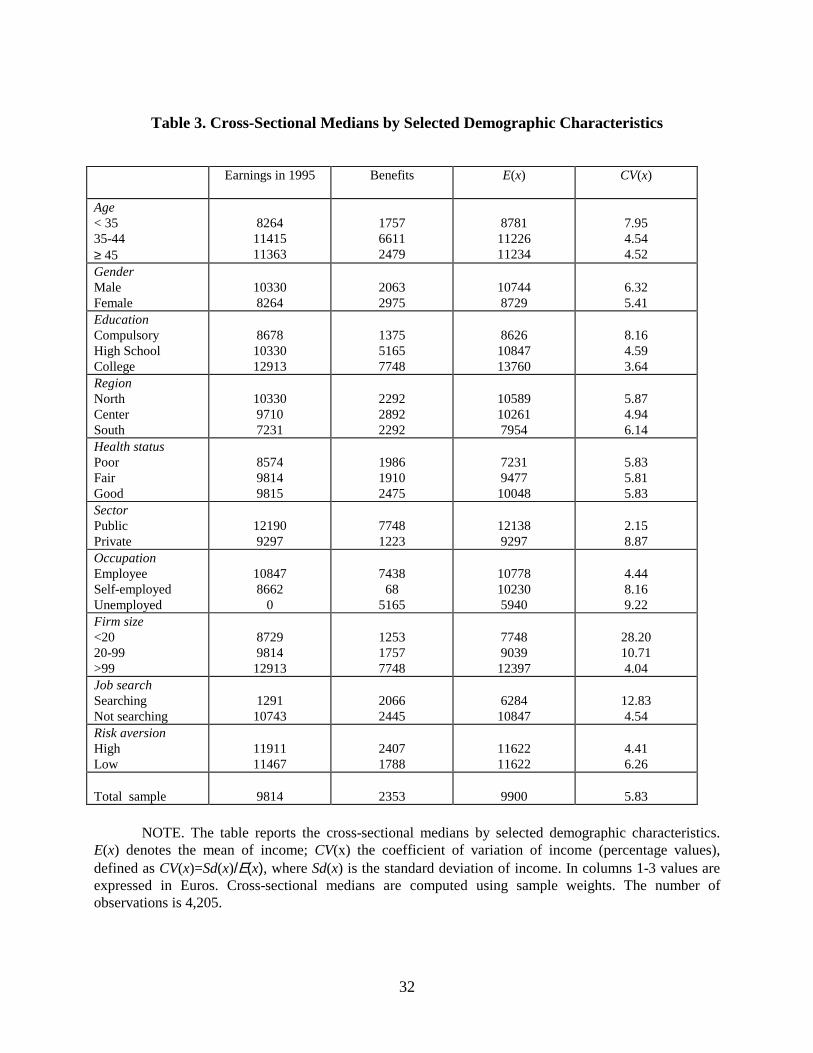
The cross-sectional medians by demographic groups of realized 1995 income, b , E(x) and
Cv(x) are reported in Table 3. Since interviews were completed between May and October of
1996, they reflect expectations stretching well into 1997, whereas income realizations refer to the
calendar year 1995. Furthermore, 1995 earnings do not include benefits, while E(x) does. The
comparison is especially misleading for the unemployed, which had no earnings in 1995 but are
assumed to receive unemployment benefits in the future. Given these caveats, on average
expected and realized income are quite close (9,814 and 9,900 Euros, respectively).
Several groups expect an income decline, particularly the elderly, people self-reporting
poor health status, and employees of small firms. The pattern of unemployment benefits across
groups reflects Italian welfare legislation program: public sector employees and employees of
large firms are more likely to receive substantial income support in the case of unemployment.
Very few welfare programs support the self-employed in case of drops in earnings.
The cross-sectional pattern of the coefficient of variation confirms that employees of the
private sector (particularly of small firms) and the self-employed perceive high risk (the median
of the coefficient of variation in the group is 8.16 percent), while public sector employees
perceive little risk (2.15 percent). Active job seekers expect more volatile incomes than those
who are not currently searching. Finally, the young and residents in the South face comparatively
more risk.
5. THE CROSS-SECTIONAL AGE-PROFILES
Income and employment uncertainty change over the life cycle. At the beginning of their
career, people face a wide range of possible opportunities involving different patterns of lifetime
earnings, but also different patterns of lifetime income uncertainty. Later on, by choice or chance
some of the original opportunities are no longer available and individuals eventually settle in jobs
with well-defined characteristics.
Knowledge of the evolution over time of earnings and employment risk matters in a
16
variety of contexts. It is important in simulation studies of lifetime wealth accumulation that
feature precautionary saving (for instance, Carroll 1997). It helps understanding the age pattern of
the composition of the household portfolio and of the willingness to hold risky assets. Insofar as
the availability of credit depends on the riskiness of income prospects, it can help understand the
age profile of households facing liquidity constraints.
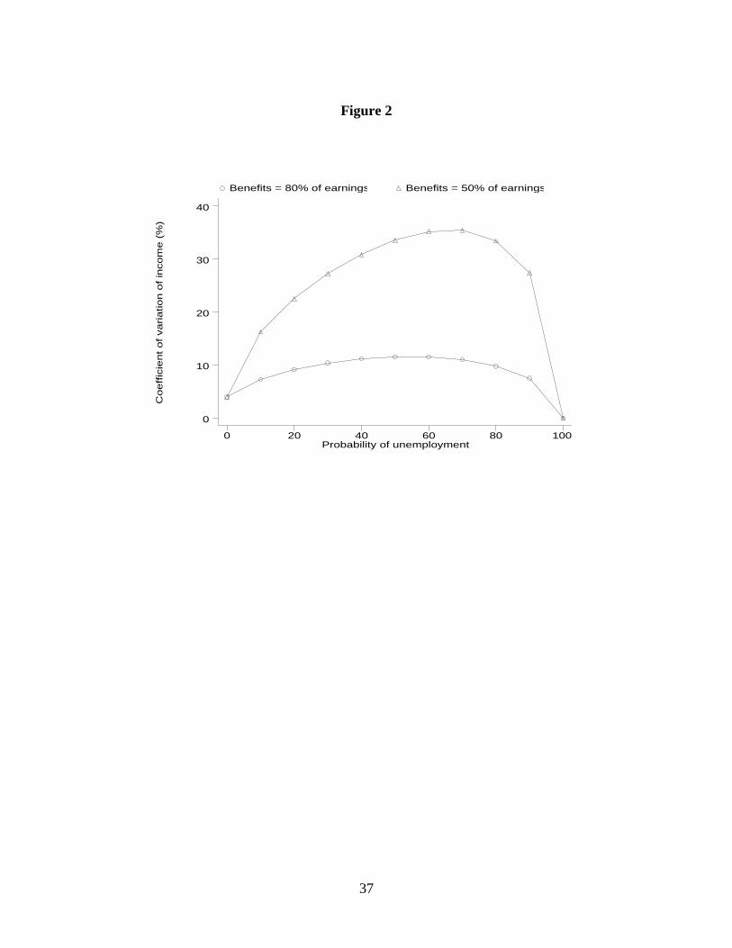
We report separate age profiles for the probability of unemployment p, the coefficient of
variation of earnings CV(y) and the coefficient of variation of income CV(x). To compute the age
profiles, we run kernel regressions for each of these variables on age using a Gaussian weight
function. Since we want to focus on the evolution of income risk over the working career, the
sample is restricted to the currently employed aged 20 to 50. The profiles are estimated for two
education groups, up to compulsory schooling and more than compulsory schooling. They
represent the effect of age on p, CV(y), and CV(x), without controlling for other age-related
individual characteristics. Since we use a pure cross-section, we make no attempt at disentangling
age effects from cohort effects.
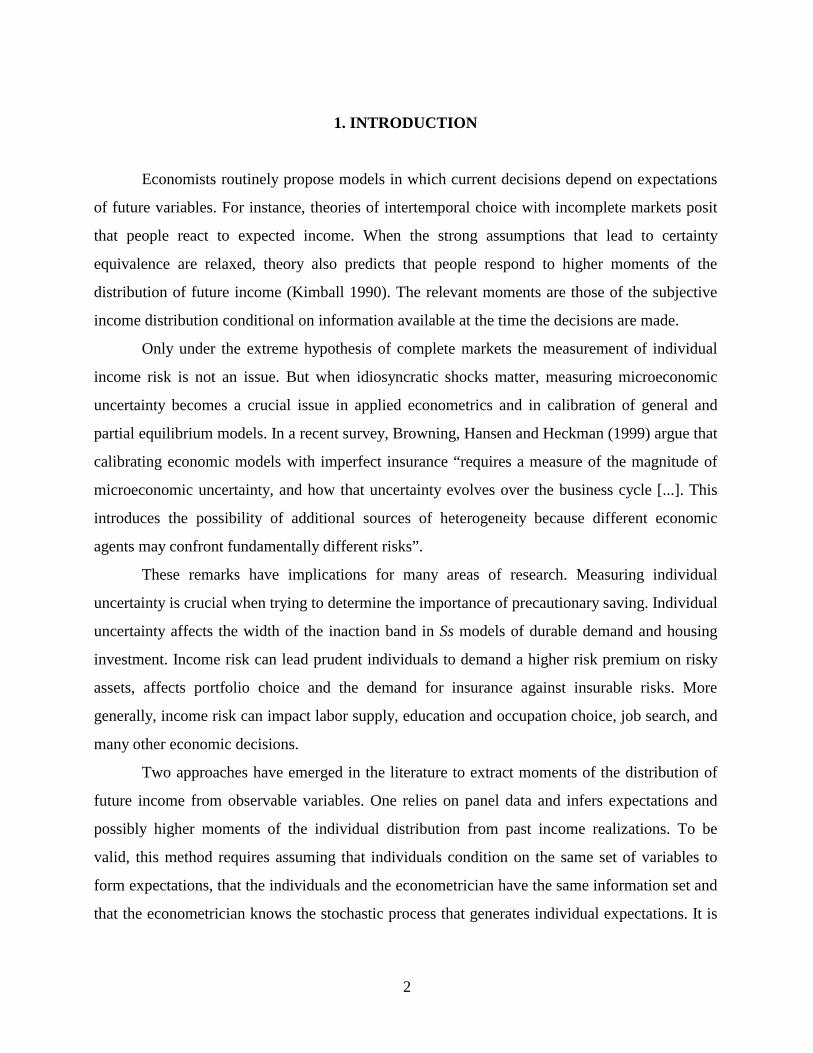
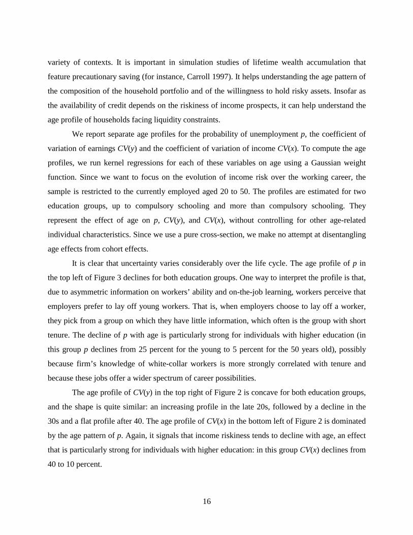
It is clear that uncertainty varies considerably over the life cycle. The age profile of p in
the top left of Figure 3 declines for both education groups. One way to interpret the profile is that,
due to asymmetric information on workers’ ability and on-the-job learning, workers perceive that
employers prefer to lay off young workers. That is, when employers choose to lay off a worker,
they pick from a group on which they have little information, which often is the group with short
tenure. The decline of p with age is particularly strong for individuals with higher education (in
this group p declines from 25 percent for the young to 5 percent for the 50 years old), possibly
because firm’s knowledge of white-collar workers is more strongly correlated with tenure and
because these jobs offer a wider spectrum of career possibilities.
The age profile of CV(y) in the top right of Figure 2 is concave for both education groups,
and the shape is quite similar: an increasing profile in the late 20s, followed by a decline in the
30s and a flat profile after 40. The age profile of CV(x) in the bottom left of Figure 2 is dominated
by the age pattern of p. Again, it signals that income riskiness tends to decline with age, an effect
that is particularly strong for individuals with higher education: in this group CV(x) declines from
40 to 10 percent.
17
6. A COMPARISON OF UNEMPLOYMENT RISK IN ITALY AND THE US
International comparison of overall income uncertainty is considered in Dominitz and
Manski (1997b) and Das and Donkers (1999). They show that perceived income uncertainty is
much higher in the US than in Europe (represented by Italy and the Netherlands). The most
natural explanation for the difference between perceived risk in Europe and the United States is
that it reflects tighter labor market regulations and more generous welfare programs in Europe.
In this section we complement their evidence by focusing instead on perceived
unemployment risk. If indeed differences in income uncertainty between the US and Europe
mainly stem from differences in labor market regulations, than they should become manifest
when comparing unemployment probabilities. This comparison could also help understand better
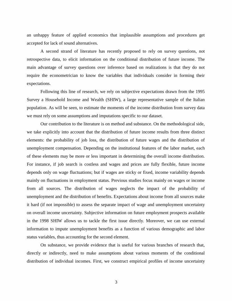
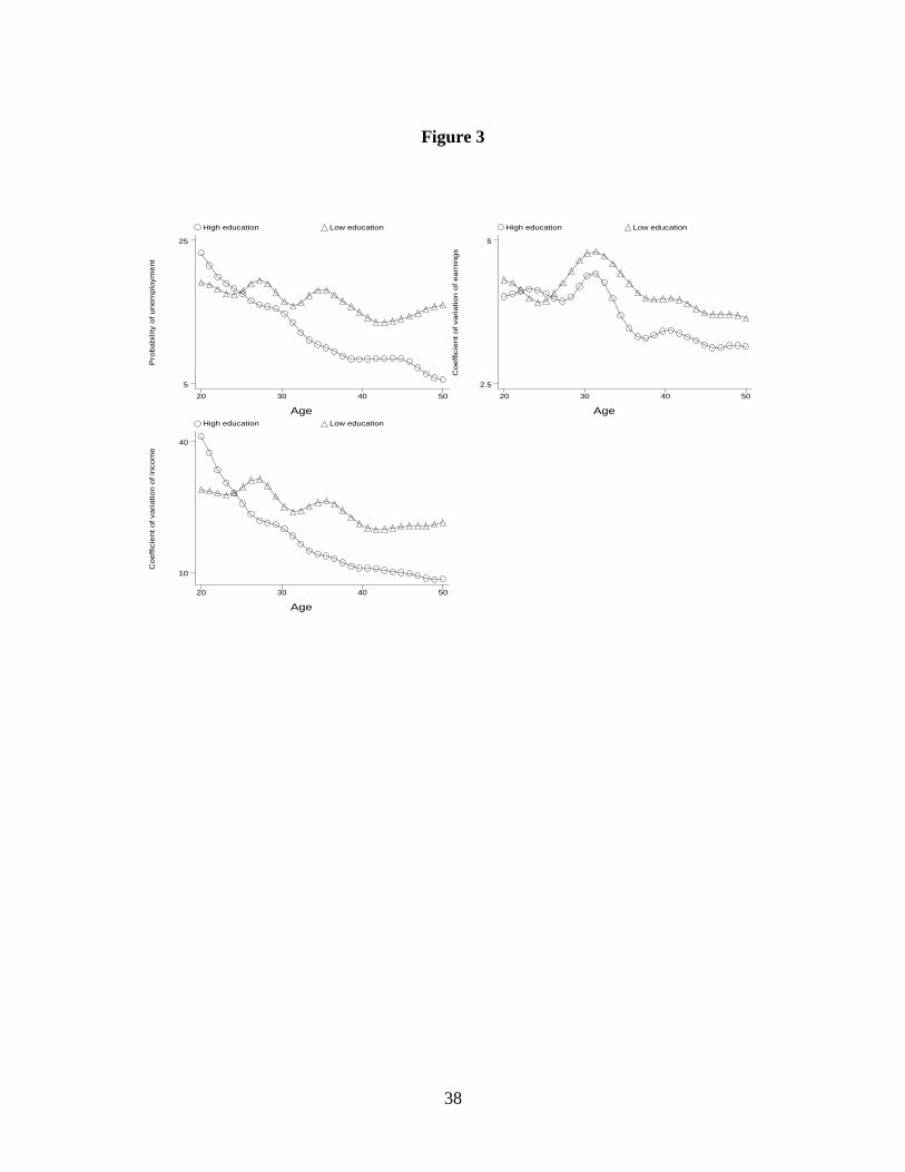
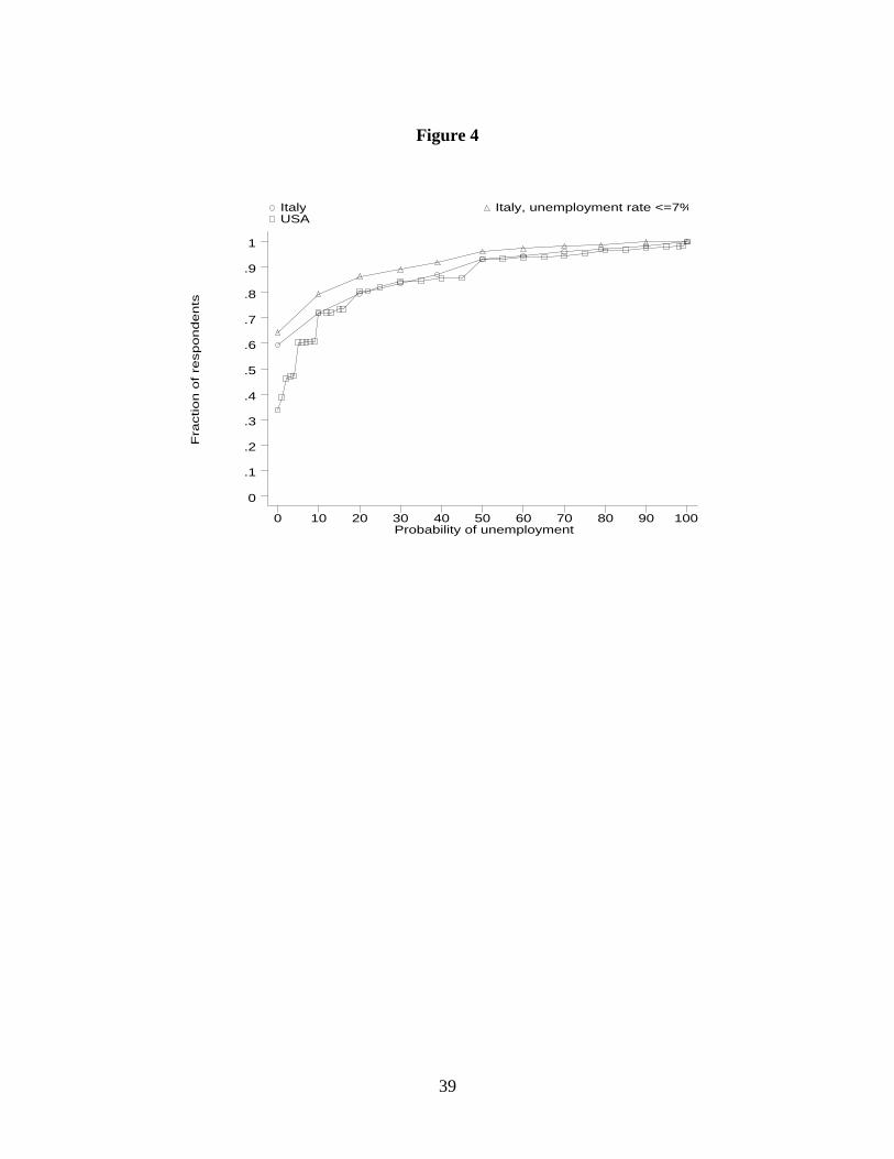
the source of the difference. In Figure 4 we report the cumulative distribution function of the
probability of unemployment in Italy and in the United States. Manski and Straub (2000) provide
data for the United States. For comparison with the US study, we focus on those currently
employed. Apart from the large difference at p=0, the two cumulative distributions are
surprisingly similar: in both countries 70 percent of individuals perceives p≤10 percent; and 10
percent faces p>60 percent. The main difference in the two distributions is at low levels of p: the
fraction of those facing no risk of job loss is much higher in Italy than in the United States (60
against 30 percent) a reflection of the different institutional characteristics of the labor market,
with a tougher job protection legislation in Italy than in the US and of the larger size and stability
of public sector’s jobs in Italy.
The comparison between the two countries could be affected by the high Italian
unemployment rates, particularly in the Southern regions. To insulate the comparison from
cyclical and structural differences in the labor market, we drop individuals living in provinces
where the unemployment rate exceeds 7 percent, leaving us with a sample in which the overall
unemployment rate is close to the 1993 US national average (we retain roughly 1,000
observations). At low levels of p the large difference between the two countries is quite
18
substantial; at higher levels of p the shape of the distribution function tends to become similar.
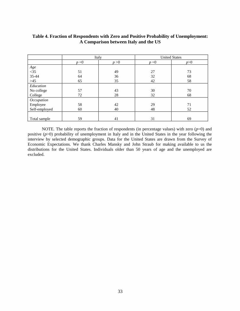
Since the difference between Italy and the United States is concentrated in the bottom part
of the p distribution, in Table 4 we focus on the demographic characteristics of the sub-samples
of those reporting p=0 and p>0. Regardless of group, the fraction of individuals reporting p=0 is
much higher in Italy. The qualitative pattern across groups is similar in the two countries: the
group with p=0 is larger for those with longer tenure (as proxied by age), those with college
education and the self-employed. But note the very high premium for job stability of Italian
college graduates: over 72 percent reports p=0 against 57 percent in the group with low
education. The comparison confirms the different nature of the two labor markets: tighter
regulation of Italian labor markets reduce substantially the employee’s perceived risk of job
dismissal relative to the United States.
There is a growing literature that compares the effect of labor market institutions on the
amount of risk that workers face, earnings inequality, and the consequent welfare effects. Bertola
and Ichino (1995) argue that labor market institutions are the main determinants of the degree of
risk perceived at the individual level. They make a strong case that workers in countries where
labor markets are highly flexible (as the United States) perceive higher income risk than workers
in countries with more rigid labor market institutions and wages (as Italy). According to Bertola
and Ichino, the probability of unemployment depends on employment status: the unemployed are
more likely to find a job and the employed are more likely to be laid off in countries with more
flexible labor markets. Using simulations, Flinn (2001) compares the implications of lifetime
welfare inequality of labor market institutions in Italy and the United States. He finds that the
American flexible system is characterized by higher cross-sectional dispersion in earnings (and
therefore higher income risk) but lower inequality in lifetime welfare, compared to the Italian
inflexible system.
Overall, the international comparison supports some of the hypothesis advanced by
Bertola and Ichino. Provided that the differences in p and overall income uncertainty do not
reflect sample design and other measurement problems, there is compelling evidence that in
countries with greater labor market flexibility on-the-job wage uncertainty is higher than in
countries with more rigid labor markets. At the same time, our analysis in this section shows that
19
for the employed p is higher in environments with more flexible labor markets; unfortunately, for
the unemployed we cannot make the comparison because we lack data for the US.
7. INCOME RISK AND RISK AVERSION
One objection to the use of income risk indicators in empirical tests of household
behavior is that coefficient estimates can be biased by self-selection. This can happen if
unobserved preferences correlate with income risk. For instance, risk-averse people may choose
low risk occupations and avoid risky jobs, such as self-employment or employment by small
firms. Consider then an applied economist who wants to estimate the importance of
precautionary saving and runs a regression of saving on income risk omitting risk aversion. The
coefficient of income risk will be biased downward by the endogeneity of the risk indicator: even
an insignificant coefficient can be consistent with precautionary saving because income risk is
negatively correlated with an omitted variable (risk aversion). See Dynan (1993) for an empirical
example and a discussion.
A question in the 1995 SHIW provides an opportunity to measure individual attitudes
towards risk and to gauge the severity of the self-selection problem. Questions on risk attitudes
are also asked in the HRS, and have been used by Barsky, Juster, Kimball, and Shapiro (1997).
Each household head in the SHIW was asked: “Suppose you have the opportunity to invest in a
risky asset. There is an equal chance that you will gain 5,000 Euros or lose everything. At most,
how much would you be willing to pay to purchase this asset?”. The expected value of such a
lottery is 5,000 Euro, and most households (95 percent) report a price that is strictly less than the
expected value of the lottery, that is they are risk averse. We then define three indicators
corresponding to low (willingness to pay strictly less than 1,250 Euro), medium (between 1,250
and 2,500) and high (2,500 or more) risk aversion.
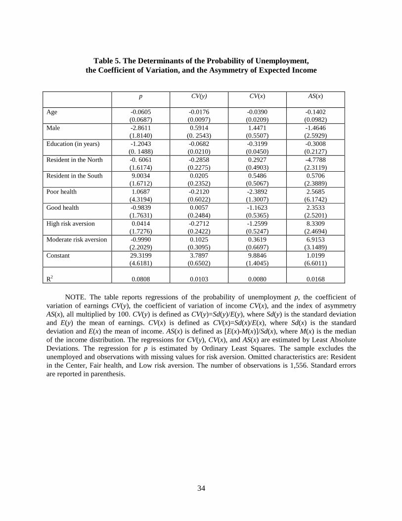
In Table 5 we regress p, CV(y), CV(x) and AS(x) on a set of demographic characteristics
and the risk aversion indicators. As the risk-aversion question is asked only to household heads
and other observations are lost because of missing or zero current earnings, the sample is
20
restricted to 1,556 individuals. If individuals self-select into jobs according to their attitudes
toward risk, their risk aversion should help predict the probability of unemployment, the
coefficient of variation, and the index of asymmetry, after controlling for individual
characteristics. In general we find the expectation variables difficult to predict on the basis of
observable characteristics, as witnessed by the low R2 reported in Table 5. This may reflect large
error in measuring income riskiness or the fact that income riskiness has a large individual
component that is not associated with standard demographic variables. However, some interesting
patterns emerge from the data.
In column (1) we focus on the probability of unemployment. As in the descriptive analysis
of Table 2, we find that p has a strong inverse correlation with education. An additional year of
education reduces the probability of unemployment by 1.2 percentage points (in this sample the
mean is 14 percent). Residence in Southern Italy, where the unemployment rate is about 3 times
the national average, has the expected effect: the thought experiment of moving an individual
from the North to the South would raise the probability of facing unemployment by roughly 10
percentage points. The coefficient of age is negative but poorly measured, and so are other
demographic characteristics. The risk aversion indicators do not explain unemployment risk.
In column (2) we relate CV(y) to the same set of variables (recall that CV(y) refers to the
earnings distribution if employed). Age and education reduce earnings variability, while being
male increases it. The coefficients of the other demographic variables and of the dummies for risk
aversion are not statistically different from zero.
The third column of Table 5 refers to CV(x). The general pattern of results is somewhat
similar to that of CV(y), with one notable exception: the coefficient of the dummy for high risk
aversion in this regression is negative and precisely estimated (a t-statistic of −2.4). The
coefficient suggests that more risk adverse individuals choose occupations where CV(x) is 1.3
percent lower than for the less risk averse (the median of CV(x) in this sub-sample is 4.22, the
mean 22). This implies that the self-selection effect cannot be easily dismissed in empirical
studies.
It is worth noting that risk aversion can be measured correctly only if income is non-
random. For instance, if the lottery is negatively correlated with income, the risk averse may be
21
willing to pay the lottery more than its fair price of 5 million lire. In our case, the hypothetical
question about risk aversion implies that the lottery is independent from income. Even if the two
risks are independent, however, the Arrow-Pratt index of risk aversion depends on income risk. If
preferences are proper in the sense of Pratt and Zeckhauser (1987), the riskier is income, the less
willing is the individual to accept an additional independent risk, the lower the price that he is
willing to pay for the lottery and the higher the index of risk aversion. This “background risk
effect” can therefore attenuate the “self-selection effect”. Empirically we find that risk aversion is
negatively correlated with CV(x), suggesting that the self-selection effect dominates. Clearly, if
the background risk effect is also present, than the true self-selection is even stronger than it
appears from our regressions.
Another important characteristic of the individual income distribution is asymmetry; for
instance, Caballero (1990) shows that the asymmetry of the distribution prompts precautionary
saving behavior. We measure the asymmetry of the income distribution with the index
[ ] ( )xSdxExMxAS )()()( −= , which ranges from –1 to 1. If AS(x)>0 the distribution is skewed
to the right, implying that very unfavorable events receive more weight than favorable events.
Intuitively, individuals who dislike negative income shocks should select themselves in
occupation with positive AS(x). In column (4) of Table 5 this intuition is confirmed. We find that
risk aversion is associated with a distribution that is skewed to the right. This implies that risk-
averse individuals select themselves into occupations where large negative income events occur
with relatively low probability. This channel adds to the selection effect due to income
uncertainty described above.
8. CONCLUSIONS
In this paper we propose a new set of indicators of expected income and subjective
income risk using the 1995 Bank of Italy Survey of Household Income and Wealth. Their main
advantage is that they are derived from simple yet powerful questions. With suitable
assumptions, these questions allow estimation of moments of the distribution of future income
22
taking into account the probability of unemployment and the distribution of unemployment
compensation. We can thus examine the entire conditional distribution of income, rather than
focusing on just one aspect, like most of the empirical literature. We point out that variations in
the perceived probability of unemployment explain a large part of the differences in income
prospects. This suggests that one should account separately for employment and income risk in
tests of households’ behavior such as consumption and portfolio choice.
The second and third moment of the income distribution and the perceived probability of
unemployment are then related to a set of demographic and preference characteristics. We find
that demographic characteristics such as age, education and geographical location affect both
unemployment risk and the variance of the subjective distribution of future earnings.
So far there is very limited evidence on the evolution of individual income risk over the
life cycle and on the effect of risk aversion on income risk (the self-selection problem). Despite
some theoretical work suggesting that asymmetry may be important for precautionary saving
(Caballero 1990), there has been no attempt at measuring higher moments of the income
distribution. We provide evidence on these issues. First of all, we find strong evidence that the
profiles of income and unemployment risk decline with age differently for individuals in different
education groups, a finding that is consistent with models of the labor market in which
asymmetric information and on-the-job-learning play an important role. Second, controlling for
demographic variables, we find that risk aversion is a predictor of income risk. This correlation
suggests that the more risk averse select themselves into occupations with low-income risk. This
finding is also consistent with the claim that the concern for security is a major factor in the
traditionally long queue of Italians seeking civil service jobs. Finally, we find that the risk averse
tend to self-select in jobs with low probability of low-income realizations.
23
Acknowledgments
We thank two anonymous referees, the Editor, Franco Peracchi and seminar participants in Rome
and Tilburg for comments on a preliminary draft of the paper. This paper is part of a research
project on “Structural Analysis of Household Savings and Wealth Positions over the Life Cycle”.
The Training and Mobility of Researchers Network Program (TMR) of the European
Commission DGXII, the Italian National Research Council (CNR), the Ministry of University
and Scientific Research (MURST), and the “Taube Faculty Research Fund” at the Stanford
Institute for Economics and Policy Research have provided financial support.

24
APPENDIX A. THE 1995 SURVEY OF HOUSEHOLD INCOME AND WEALTH The 1995 Survey of Household Income and Wealth (SHIW) has data on income, consumption, financial wealth, real estate wealth, and several demographic variables for a representative sample of 8,135 Italian households (including 14,699 income recipients). Interviews were conducted between May and October of 1996. Balance-sheet items are end-1995 values. Income and flow variables refer to 1995. The survey also covers job search activity, hours of work and labor force participation. Brandolini and Cannari (1994) describe the main features of the SHIW, its sample design, interviewing procedure and response rates. Details about the 1995 sample can be found in Banca d’Italia (1997). The dataset can be obtained by writing to: Banca d’Italia, Research Department, Via Nazionale 91, 00196 Rome, Italy. APPENDIX B. THE QUESTIONS ON INCOME EXPECTATIONS
The 1995 SHIW contains two special sections, respectively on subjective income expectations and past labor market experience. To reduce overall interview time, half of the sample is asked questions from the first section and the other half questions from the second section. Allocation of households to the two sections is random and based on the year of birth of the head (odd or even).
Four questions on income expectations were thus asked to half of the overall sample after excluding the currently retired and people not in the labor force (a total of 4,799 individuals). Both the employed, the unemployed and the job seekers are asked to state, on a scale from 0 to 100, their chances of having a job in the 12 months following the interview. Each individual assigning a positive probability to being employed is then asked to report the minimum (ym) and the maximum (yM) incomes he or she expects to earn if employed, and the probability of earning less than the midpoint of the support of the distribution, Prob(y ≤ (ym+ yM)/2) = π. The exact wording of the survey questions is provided below. All respondents are first asked: (i) “Do you expect to voluntarily retire or stop working in the next 12 months?” If the answer is “Yes” the interviewer goes on to the next survey section. If the answer is “No” each respondent is asked questions (ii) through (v) below:

25
(ii) “What are the chances that in the next 12 months you will keep your job or find one (or
start a new activity)? In other words, if you were to assign a score between 0 and 100 to the chance of keeping your job or of finding one (or of starting a new business), what score would you assign? (“0” if you are certain not to work, “100” if you are certain to work). The following table is shown to the respondent:
.... .... .... .... .... .... .... .... .... ....
0 10 20 30 40 50 60 70 80 90 100 I am sure that
I will not have a job
I am sure that I will have a job
(iii) Suppose you will keep your job or that in the next 12 months you will find one. What is
the minimum annual income, net of taxes and contributions that you expect to earn from this job?
(iv) Again suppose you will keep your job or that in the next 12 months you will find one.
What is the maximum annual income, net of taxes and contributions that you expect to earn from this job?
(v) What are the chances that you will earn less than X (where X is computed by the
interviewer as [(iii)+(iv)]/2)? In other words, if you were to assign a score between 0 and 100 to the chance of earning less than X, what score would you assign? (“0” if you are certain to earn more than X, “100” if you are certain to earn less than X). The following table is shown to the respondent:
.... .... .... .... .... .... .... .... .... ....
0 10 20 30 40 50 60 70 80 90 100 I am sure that
I will earn more than X
I am sure I will earn less than X
APPENDIX C: IMPUTATION OF UNEMPLOYMENT BENEFITS
Under the Italian welfare programs in place in 1995-96, unemployment benefits depend on labor market status and individual characteristics. We separate the sample into four main groups: first-job seekers, long-term unemployed, currently employed, and self-employed. In principle,
26
first-job seekers, long-term unemployed, and the self-employed are not entitled to benefits. However, they may be eligible for special welfare programs offering part-time jobs. For individuals in these groups we impute, by region, an average benefit equal to the ratio between 1995 public expenditure on these special welfare programs and the number of first-job seekers. Data are drawn from Alfredo Casotti and Maria Rosa Gheido (1997), “Lavori socialmente utili,” Diritto e Pratica del Lavoro, 28. Rome: IPSOA.
Only the currently employed receive an explicit compensation in case of temporary lay-off. Unemployment compensation depends on gross earnings at the time of lay-off and on firm size. Benefit duration varies by firm size. Following current legislation, we use the following values:
- for those working in firms with over 50 employees and earning a gross monthly salary
above 2.5 million lire, unemployment benefits are set at 1.5 million lire a month, and are received for twelve months following the lay-off;
- for those working in firms with over 50 employees and earning a gross monthly salary below 2.5 million lire, benefits are set either at 1.25 million lire monthly or 80 percent of gross salary, whichever is the less (duration is again 12 months);
- for those working in small firms (under 50 employees), benefits are set at 30 percent of gross monthly income, and are received for 6 months.
Finally, we set unemployment benefits equal to minimum earnings (ym) when the former
exceeds the latter. APPENDIX D: THE TRIANGULAR DISTRIBUTION Assume that the earnings distribution is triangular over the two intervals [ym, (ym+yM)/2] and ((ym+yM)/2, yM]. The probability mass to the left of the midpoint (ym+yM)/2 is constrained to be equal to π as in Figure 2.The density function of the distribution is:
f(y)= 82
81
22 2π π( )
( )( ) ( )( )
( )( )y y
y yy y
y y y yy y
y yy ym
M mm
m M M
M m
m MM
−−
≤ <+
+− −
−+
≤ ≤
1 1
and the mean and variance of earnings are:
E(y)= π3
(2ym+ yM)+ 13− π ( ym+2yM)
Var(y)= π24
(11ym2+10ymyM+3yM
2)+ 124− π (3ym
2+10ymyM+11yM2) - [E(y)]2
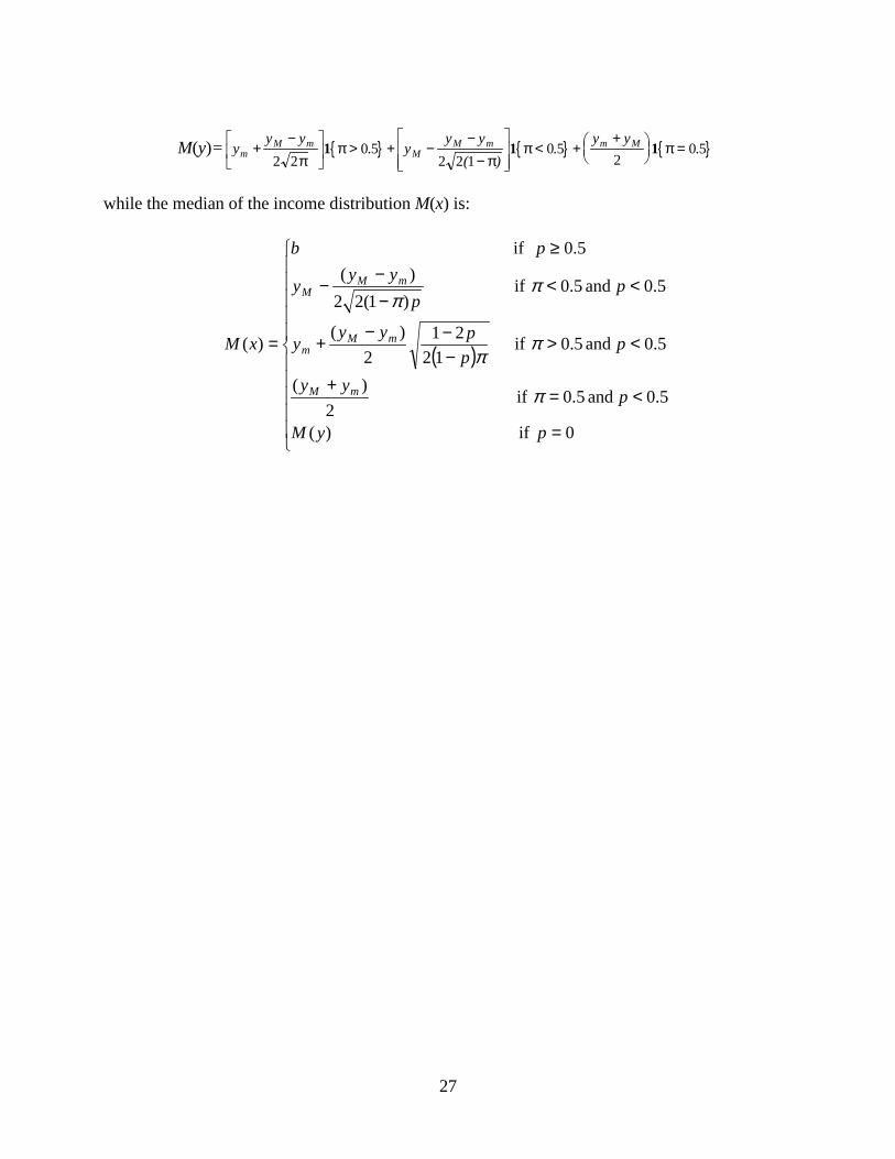
E(x) and Var(x) are then computed using equations (6) and (7) in the text. The median of the distribution of earnings M(y) is given by:
27
M(y)= { } { } { }yy y
yy y y y
mM m
MM m m M+
−
> + −
−−
< ++
=
2 20 5
2 2 10 5
20 5
ππ
ππ π1 1 1.
( ). .
while the median of the income distribution M(x) is:
( )
=
<=+
<>−−−
+
<<−−
−
≥
=
0 if )(
0.5 and 0.5 if 2
)(
0.5 and 0.5 if 12
212
)(
0.5 and 0.5 if )1(22)(
5.0 if
)(
pyM
pyy
pppyy
y
pp
yyy
pb
xM
mM
mMm
mMM
π
ππ
ππ
28
References
Banca d’Italia (1997), “I Bilanci delle Famiglie Italiane Nell’Anno 1995,” Supplemento al Bollettino Statistico, n. 14, March.
Barski, R. B., Juster, T., Kimball, M. S., and Shapiro M. D. (1997), “Preference parameters and behavioral heterogeneity: an experimental approach in the Health and Retirement Survey,” Quarterly Journal of Economics 112, 537-80.
Bertola, G., and Ichino A. (1995), “Wage Inequality and Unemployment: United States vs. Europe,” NBER Macroeconomics Annual 1995. Cambridge: MIT Press
Brandolini, A., and Cannari L. (1994), “Methodological Appendix,” in Saving and the Accumulation of Wealth, eds. A. Ando, L.Guiso and I. Visco, Cambridge: Cambridge University Press.
Browning, M., Hansen L., and Heckman J. (1999), “Microdata and General Equilibrium Models,” in Handbook of Macroeconomics, eds. J. B. Taylor and M. Woodford. Amsterdm: North-Holland.
Caballero, R. (1990), “Consumption Puzzles and Precautionary Saving,” Journal of Monetary Economics, 25, 113-36.
Das, M., and Donkers B. (1999), “How Certain are Dutch Households About Future Income? An Empirical Analysis,” Review of Income and Wealth, 45, 325-338.
Dominitz, J. (1998), “Earnings Expectations, Revisions, and Ralizations,”Review of Economics and Statistics, 374-88.
______, and Manski C. F. (1997a), “Using Expectations Data to Study Subjective Income Expectations,” Journal of the American Statistical Association, 92, 855-67.
______, and _____ (1997b), “Perceptions of Economic Insecurity: Evidence from the Survey of Economic Expectations,” Public Opinion Quarterly, 61, 261-87.
Dynan, K. (1993), “How Prudent are Consumers?,” Journal of Political Economy, 101, 1104-13.
Flinn C. J. (2001), “Labor Market Structure and Inequality: A Comparison of Italy and the US,” New York University, Dept. of Economics, unpublished manuscript.
Guiso, L., Jappelli T., and Terlizzese D. (1992), “Earnings Uncertainty and Precautionary Saving,” Journal of Monetary Economics, 30, 307-337.
Kimball, M. S. (1990), “Precautionary Saving in the Small and in the Large,” Econometrica, 58, 53-73.
29
MaCurdy, T. E. (1982), “The Use of Time Series Processes to Model the Error Structure of Earnings in a Longitudinal Data Analysis,” Journal of Econometrics, 18, 82-114.
Manski, C. F., and Straub J. D. (2000), “Worker Perceptions of Job Insecurity in the Mid-1990s: Evidence from the Survey of Economic Expectations,” Journal of Human Resources, 35, 447-480.
Pratt, J. W., and Zeckhauser R. (1987), “Proper Risk Aversion,” Econometrica, 55, 143-154.
30
Table 1. Deciles of the Cross-Sectional Distribution of the Probability of Unemployment and of the Coefficient of Variation
Deciles p CV(y) CV(x)
I 0 0.00
0.00
II 0 0.99
1.24
III 0 1.67 2.14
IV 0 2.24
3.71
Median 10 3.14
5.83
VI 10 3.87 10.21
VII 30 4.91 18.00
VIII 50 6.26
39.64
IX 80 8.84
75.17
Mean 22.13 4.13
24.29
NOTE. The table reports percentage values of the deciles of the cross-sectional distributions of the probability of unemployment, the coefficient of variation of earnings and the coefficient of variation of income. The coefficient of variation of earnings is defined as CV(y)=Sd(y)/Ε(y), where Sd(y) is the standard deviation and E(y) the mean of earnings. The coefficient of variation of income is defined as CV(x)=Sd(x)/E(x) where Sd(x) is the standard deviation and E(x) the mean of income; mean and standard deviation in this case take into account the probability of unemployment and expected benefits. The number of observations is 4,205. All statistics are computed using sample weights.
31
Table 2. Probability of Unemployment by Selected Demographic Characteristics
Unemployed in 1995 Employed in 1995 Whole sample Age < 35 35-44 ≥ 45
61.82 59.46 76.50
17.61 13.01 13.62
27.86 15.99 18.81
Gender Male Female
65.50 61.10
14.50 15.96
21.63 22.90
Education Compulsory High School College
67.19 61.67 49.26
18.31 12.81 8.84
26.13 19.43 13.50
Region North Center South
50.10 60.10 69.75
11.75 12.73 22.57
14.28 19.66 34.80
Health status Poor Fair Good
62.45 78.83 63.43
22.66 15.19 14.89
32.67 23.26 21.77
Sector Public Private
- -
9.29
17.34
9.29
17.34 Firm size <20 20-99 >99
- - -
21.30 19.94 10.69
21.30 19.94 10.69
Job search Searching Not searching
62.57 68.32
29.38 13.44
48.44 15.36
Risk aversion High Low
66.91 72.80
13.62 13.63
17.47 17.85
Sample average
63.67
15.06
22.13
Number of observations
659
3,546
4,205
NOTE. The table reports percentage values of the average probability of unemployment in the year following the interview by selected demographic groups. All means are computed using sample weights.
32
Table 3. Cross-Sectional Medians by Selected Demographic Characteristics Earnings in 1995 Benefits E(x) CV(x)
Age < 35 35-44 ≥ 45
8264
11415 11363
1757 6611 2479
8781
11226 11234
7.95 4.54 4.52
Gender Male Female
10330 8264
2063 2975
10744 8729
6.32 5.41
Education Compulsory High School College
8678
10330 12913
1375 5165 7748
8626
10847 13760
8.16 4.59 3.64
Region North Center South
10330 9710 7231
2292 2892 2292
10589 10261 7954
5.87 4.94 6.14
Health status Poor Fair Good
8574 9814 9815
1986 1910 2475
7231 9477
10048
5.83 5.81 5.83
Sector Public Private
12190 9297
7748 1223
12138 9297
2.15 8.87
Occupation Employee Self-employed Unemployed
10847 8662
0
7438
68 5165
10778 10230 5940
4.44 8.16 9.22
Firm size <20 20-99 >99
8729 9814
12913
1253 1757 7748
7748 9039
12397
28.20 10.71 4.04
Job search Searching Not searching
1291
10743
2066 2445
6284
10847
12.83 4.54
Risk aversion High Low
11911 11467
2407 1788
11622 11622
4.41 6.26
Total sample
9814
2353
9900
5.83
NOTE. The table reports the cross-sectional medians by selected demographic characteristics. E(x) denotes the mean of income; CV(x) the coefficient of variation of income (percentage values), defined as CV(x)=Sd(x)/Ε(x), where Sd(x) is the standard deviation of income. In columns 1-3 values are expressed in Euros. Cross-sectional medians are computed using sample weights. The number of observations is 4,205.
33
Table 4. Fraction of Respondents with Zero and Positive Probability of Unemployment: A Comparison between Italy and the US
Italy United States p =0 p >0 p =0 p>0 Age <35 35-44 >45
51 64 65
49 36 35
27 32 42
73 68 58
Education No college College
57 72
43 28
30 32
70 68
Occupation Employee Self-employed
58 60
42 40
29 48
71 52
Total sample
59
41
31
69
NOTE. The table reports the fraction of respondents (in percentage values) with zero (p=0) and positive (p>0) probability of unemployment in Italy and in the United States in the year following the interview by selected demographic groups. Data for the United States are drawn from the Survey of Economic Expectations. We thank Charles Mansky and John Straub for making available to us the distributions for the United States. Individuals older than 50 years of age and the unemployed are excluded.
34
Table 5. The Determinants of the Probability of Unemployment, the Coefficient of Variation, and the Asymmetry of Expected Income
p CV(y) CV(x)
AS(x)
Age -0.0605 (0.0687)
-0.0176 (0.0097)
-0.0390 (0.0209)
-0.1402 (0.0982)
Male
-2.8611 (1.8140)
0.5914 (0. 2543)
1.4471 (0.5507)
-1.4646 (2.5929)
Education (in years) -1.2043 (0. 1488)
-0.0682 (0.0210)
-0.3199 (0.0450)
-0.3008 (0.2127)
Resident in the North -0. 6061 (1.6174)
-0.2858 (0.2275)
0.2927 (0.4903)
-4.7788 (2.3119)
Resident in the South 9.0034 (1.6712)
0.0205 (0.2352)
0.5486 (0.5067)
0.5706 (2.3889)
Poor health 1.0687 (4.3194)
-0.2120 (0.6022)
-2.3892 (1.3007)
2.5685 (6.1742)
Good health -0.9839 (1.7631)
0.0057 (0.2484)
-1.1623 (0.5365)
2.3533 (2.5201)
High risk aversion 0.0414 (1.7276)
-0.2712 (0.2422)
-1.2599 (0.5247)
8.3309 (2.4694)
Moderate risk aversion
-0.9990 (2.2029)
0.1025 (0.3095)
0.3619 (0.6697)
6.9153 (3.1489)
Constant 29.3199 (4.6181)
3.7897 (0.6502)
9.8846 (1.4045)
1.0199 (6.6011)
R2
0.0808
0.0103
0.0080
0.0168
NOTE. The table reports regressions of the probability of unemployment p, the coefficient of variation of earnings CV(y), the coefficient of variation of income CV(x), and the index of asymmetry AS(x), all multiplied by 100. CV(y) is defined as CV(y)=Sd(y)/E(y), where Sd(y) is the standard deviation and E(y) the mean of earnings. CV(x) is defined as CV(x)=Sd(x)/E(x), where Sd(x) is the standard deviation and E(x) the mean of income. AS(x) is defined as [E(x)-M(x)]/Sd(x), where M(x) is the median of the income distribution. The regressions for CV(y), CV(x), and AS(x) are estimated by Least Absolute Deviations. The regression for p is estimated by Ordinary Least Squares. The sample excludes the unemployed and observations with missing values for risk aversion. Omitted characteristics are: Resident in the Center, Fair health, and Low risk aversion. The number of observations is 1,556. Standard errors are reported in parenthesis.
35
Figure Captions
Figure 1. The Triangular Distribution of Earnings. Figure 2. The Effect of the Probability of Unemployment on the Coefficient of Variation of Income. The figure reports the relation between the probability of unemployment and the coefficient of variation of income CV(x). In the examples average earnings E(y) and the variance of earnings Var(y) are set at 100 and 16 respectively. In the upper line unemployment benefits are set at 80 percent of E(y), in the lower line at 50 percent. Figure 3. Age Profiles of the Probability of Unemployment, Earnings and Income. The age profiles are estimated by a kernel regression using a Gaussian weight function. Each regression is estimated separately for employed workers who completed junior high school (low education) and those who completed high school or college (high education). Figure 4. The Probability of Unemployment in Italy and the United States. The figure reports the subjective probability of unemployment in Italy and the United States. Data for the United States are drawn from the 1994-1998 Survey of Economic Expectations (SEE), see Manski and Straub (2000). The higher line for Italy excludes individuals living in provinces where the average unemployment rate (drawn from aggregate labor force statistics) exceeds 7 percent in 1995.
36
Figure 1
f(y)
π 1−π
ym yM(ym+yM)/2
8π(y−ym)/(yM−ym)2
8(1−π)(yM−y)/(yM−ym)2
y
37
Figure 2
Coe
ffic
ient
of
varia
tion
of in
com
e (%
)
Probability of unemployment
Benefits = 80% of earnings Benefits = 50% of earnings
0 20 40 60 80 100
0
10
20
30
40
38
Figure 3
Pro
babi
lity
of u
nem
ploy
men
t
Age
High education Low education
20 30 40 505
25
Coe
ffici
ent o
f var
iatio
n of
ear
ning
s
Age
High education Low education
20 30 40 502.5
5
Coe
ffici
ent o
f var
iatio
n of
inco
me
Age
High education Low education
20 30 40 50
10
40
39
Figure 4
Fra
ctio
n o
f re
spondents
Probability of unemployment
Italy Italy, unemployment rate <=7% USA
0 10 20 30 40 50 60 70 80 90 100
0
.1
.2
.3
.4
.5
.6
.7
.8
.9
1