an empirical analysis of the exchange rate regime in the republic of...

International Journal of Academic Research in Economics and Management Sciences (November) 2013, Vol. 2, No. 6

ISSN: 2226-3624

135 www.hrmars.com/journals

An Empirical Analysis of the Exchange Rate Regime in the Republic of Macedonia

Murat Sadiku, PhD

Department of Business and Economics, South East European University Republic of Macedonia, Email: [email protected]

Fluturim Saliu, PhD Department of Economics, State University of Tetovo

Republic of Macedonia

Luljeta Sadiku, PhD candidate Department of Economics, State University of Tetovo

Republic of Macedonia

DOI: 10.6007/IJAREMS/v2-i6/490 URL: http://dx.doi.org/10.6007/IJAREMS/v2-i6/490

Abstract

Fixed or floating exchange rate regime is one of dilemmas that arise between economic scholars and policymakers. Republic of Macedonia as a small opened economy has adopted the fixed exchange regime, but there are studies’ conclusions that the country pays considerable costs in maintaining the fixed exchange regime. Therefore the purpose of this research paper is to answer the question by an empirical analysis if Macedonia needs to maintain the fixed exchange regime or should change the regime to floating. To examine this, we analyze the effects of a range of macroeconomic variables such as real GDP, government fiscal balance, retail price index, trade openness, current account balance and monetary aggregates on the real effective exchange rate. In order to allow interaction between above variables a co-integration test has been done for ascertaining the short and long run relationship. Also the Granger Causality test has been applied to determine if causal relationship exists between variables. Based on vector error correction method (VECM) results, real GDP, trade openness, current account and monetary aggregates do not have significant effect on the real effective exchange rate in the long run. Regarding the retail price index and government balance are significant determinants in the short as well as long run dynamics. Thus, the empirical results reveal some relevant arguments that support the fix exchange regime.

Key words: Real exchange rate, macroeconomic variables, co-integration, causality

1. Introduction

The optimal exchange rate and monetary regimes have been an issue of discussion since the beginning of the ‘70th with the breakdown of Bretton Woods’s system. There is a large body of theoretical and empirical research that attempt to identify which one is more appropriate for developed and least


ISSN: 2226-3624


developed market economies1. However, the determination of the regime of the exchange rate for the countries in transition has been substantially different compare to the developed ones.

The early researches of Mundell’s (1961) and McKinnon (1963) argue that economic size and openness are the fundamental determinants affecting a countries exchange regime of choice. He points out that small and open economies are more likely to adopt fixed exchange rates regime than large and relatively closed economies. Also some more recent studies confirm that the determinants of the choice of the exchange rate regime in transition economies should have into consideration the economic size and geographical concentration of trade (Markiewicz, A. 2006; Hagen J.& Zhou, J.). Moreover, some other studies reflect that: international financial market integration, macroeconomic performance, financial sector development, and political economy considerations are important fundamentals.

Melvin (1985) proposed that countries that are subject to “real shocks”-for instance raw material exporters-would benefit more from flexible exchange rate which might be necessary to fulfill the external condition of competitiveness maintained. On the other side, countries that were seen as prone to “nominal shocks”, for instance unstable monetary conditions would benefit more from fixed exchange rates that allows credibility.

Republic of Macedonia as a small opened economy has adopted the fixed exchange regime, but it is questionable if the country ‘pays’ considerable costs in maintaining the fixed exchange regime. Therefore the purpose of this research paper is to answer the question if Macedonia needs to maintain the fixed exchange regime or should change the regime to floating? To examine this, we analyse the effects of a range of macroeconomic variables such as real GDP, retail price index (RPI), government fiscal balance, trade openness, current account and monetary aggregates on the real effective exchange and vice-versa, the effects of the exchange rate on the above variables using the Granger causality Wald test. The vector error correction method (VECM) is used to analyze these potential determinants by taking into consideration also the structural shocks2. Based on VECM results trade openness, current account and monetary aggregates do not have significant effect on the real effective exchange rate in the short run as well as long run. Regarding the retail price index and government balance are significant in the short as well as long run dynamics. Real GDP is significant only in the short run. Also the Granger causality tests are designated if the causal relationships exist between variables after running a vector auto regression (VAR) model. The results from the test indicate that there is not a causal relationship between exchange rate and trade openness as well as exchange rate, current account and monetary aggregates, respectively. Thus, the empirical results reveal some relevant arguments that support the fix exchange regime.

2. Exchange Rate Movements and Economic Performance in Republic of Macedonia

In the early 1990’s Macedonia’s economy was characterized as a lower income economy, due to the deep drop in GDP accompanied by high inflation rates. Over the last 10 years, Macedonia had an average of 3 percent growth rate. During 1996, Macedonia’s economy stabilized and the real growth was 1.2 percent, followed by 4.5 percent in 2000, but the 2001 ethnic conflict resulted in a negative growth rate of -4.5 percent. The highest growth rate of 6.1 percent was recorded in 2007. Increase in exports and higher household consumption are said to have accounted for this upsurge in GDP growth.

1 For comprehensive details see: Ghosh et al. (1997); Frankel (1999); Moosa (2005); Mundell (1961); McKinnon

(1963) 2 With structural shocks we mean an event in a particular time period, like currency crisis, war, restrictive

government policies etc.


ISSN: 2226-3624


Recently, while several indicators have shown significant improvement, the global financial crisis has affected the economy of Macedonia driven by a decline in the output of the metal and textile sectors, which are the main export earners. As a result the GDP growth in 2009 was again negative at -0.9 percent. The economy slowly started to recover in 2010 as real GDP grew by 1.8 percent.

From 1997-2012, the rate of inflation has been a single-digit number, so monetary policy strategy of targeting the exchange rate has proven very successful on stabilization price’s level of the economy. However, other macroeconomic variables are not considered in a favorable situation. For example, high deficit of current account of the balance of payment, low foreign direct investments and low economic growth (see Figure 1).

Figure 1. Real GDP growth, Current Account Balance and FDI in RM

-10

-50

51

01

5

1998q1 2001q3 2005q1 2008q3 2012q1

Current account balance (% of GDP) % Real GDP growth

FDI (% of GDP)

Quarterly data of Real GDP Growth, Current account Balance and FDI in RM

Source: State Statistical Office of RM and National Bank of RM

Even though Macedonia was facing systematic changes such as joining the World Trade Organization (2002), liberalization of the capital account (2003), and the application for joining the European Union (2004), the global financial crisis of 2008 caused high macroeconomic instability such as: currency crisis from the speculative attacks of the Denar3 which were overcome through high sale of the foreign reserves on the foreign exchange market by the Central Bank in the last quarter of 2008 and first quarter of 2009. On the other hand, this action was melting down the foreign reserves causing a rise of public debt. This was accompanied by a decrease in the Denar deposits, while have increased the deposits in Euro creating pressures for devaluation of the Denar.

From 1995 up to the date, the Central Bank of the country has implemented the targeting strategy of the exchange rate by using Deutschmark in the beginning and after Euro as a nominal anchor. Implementing this strategy to transmit the effects of the monetary policy in the economy has been followed by positive achievements until the third quarter of 2008. Even during the events in Kosovo in

3 Denar is the national currency of the Republic of Macedonia


ISSN: 2226-3624


1999 and the ethnic strive of 2001, the stability of the exchange rate was maintained.4 But, the global economic crisis has brought up a frequent debate issue among the economists of whether to abandon or keep the fix exchange rate that has been melting down the foreign reserves of the state. So, to avoid further devaluation of the Denar the Central Bank intervenes in the foreign exchange market by selling Euro in exchange for Denars in order to defend the stability of the exchange rate.5

The Central Bank of Macedonia has continued to implement the strategy of targeting the nominal exchange rate of Denar relative to the Euro. Thus, the nominal exchange rate of the Denar relative to the Euro has continued to represent an intermediate target of the monetary policy.6 The foreign exchange transactions of the Central Bank in reality represented an important way to withdraw the excess liquidity from the banking sector. By maintaining a stable exchange rate the Central Bank achieves its ultimate goal of price stability. In 2006, the inflation increased at about 3.2% (as shown in the Figure 2. below), which was mainly caused by a combination of the high prices in energy. On the other side 2007 is characterized with an average inflation of 2.3%, which was lower by 0.9% compare to the previous year and this is as result of the gradual regulation in excise taxes. But beginning from July of 2007 the seasonal dryness caused year by year the increase in inflation which reached an average level of 8.3% in 2008. Major factors that increased inflation in first half of the year were the higher food and energy prices. The rise in domestic prices was paralleled with the increase of the prices in many other economies in the world as well.

Figure 2. The Movement of Inflation and exchange rate over years

60.6

60.8

61.0

61.2

61.4

61.6

-2%

0%

2%

4%

6%

8%

10%

20002001

20022003

20042005

20062007

20082009

20102011

2012

Exchange rate Inflation

Source: National Bank of Republic of Macedonia

4 See Belke.A & Zenkić.A (2006), ‘Exchange Rate Regimes and the Transition Process in the Western Balkans’,

Paper prepared for the 3rd

Euro frame Conference on Policy Issues in EU-Towards an Enlarging EMU: Challenges for New and Old Member States, pg. 23. 5 See for details Nenovski T. & Makrevska E.( 2009), ‘Influence of the Economic Crisis on the Exchange Rates of the

Countries from Eastern and Central Europe’, Fourth Annual International Conference on European Integration EUROPE IN CRISIS: THREATS AND OPPORTUNITIES, University American College-Skopje 2009 pg. 178-182; 6 NBRM(2004), Annual Report , Published April/2005


ISSN: 2226-3624


The Central Bank in order to calm down the inflation expectations and to reduce the pressure for a devaluation of the Denar in the fourth quarter of 2008 intervened on the foreign exchange market with net sale of foreign assets. The total net sell of foreign reserves in 2008 was 0.9% of the GDP.7 The main factors that contributed to the negative change in the general price level in 2009 were: the cut of the oil derivative prices and the decrease in the costs for car maintenance and the prices of the transport equipment. So, the global recession interrupted the increase in import prices that caused disinflation of 0.8% in Macedonian economy. Until March of 2009, the Central Bank intervened in the foreign exchange market by selling foreign reserves and by increasing the basic interest rate stabilized the exchange rate.

3. A Brief Literature Review of the Empirical Evidence of the Exchange Rate Regime

Many studies reflect the linkage between exchange rate regime and macroeconomic variables, but the relationship and influence is different among studies and countries. In this section is outlined a brief literature review on the effects of the exchange rate on macroeconomic variables.

Certainly, one of the most prominent studies on the empirical evidence of the exchange rate was conducted by Ghosh et al. (1997) for 145 countries during 1960-1990. They found a slightly higher GDP growth under float, 1.7% compared to 1.4% under peg. But the highest growth 2% is under managed float or intermediate regime. On the other side, Moreno (2000, 2001) for 98 developing East Asian countries, in both studies finds that the difference in GDP growth between regimes significantly narrows. He supports that the real growth under peg is higher respectively by 1.1% and 3.3%. Moreover, Levy-Yeyati and Sturzenegger (2000) for 183 countries found that countries with fixed exchange rate regimes have had a lower rate per-capita growth ranging between 0.66% and 0.88% compare to the flexible regime. While the empirical analysis of Husain et al (2004) for 158 countries, suggest that neither pegs harm growth nor flexible regimes support growth.

Cîtu (2003) takes a different approach for New Zeland. By a VAR methodology he examines that Exchange rate plays a significant role in transmitting the effects of monetary policy in smaller developed countries and not in the big developed countries. Also, Disyatat (2001) uses the same method for Asian & ERM countries and points out that unanticipated exchange rate depreciation could really reduce GDP growth because high share of debt in the economy is denominated in foreign currency. Furthermore Coricelli, Jazbec & Masten for Czech Republic, Hungary, Poland and Slovenia found that exchange rate pass-through effect on domestic prices remains relevant even during the advanced stages of transition in the EU candidate countries.

Concerning the Republic of Macedonia several studies were carried out on this subject, for example, Krstevska et al (2003) reported a lower pass-through of 0.10% on the prices given the greater stability of the exchange rate. While Besimi et al. (2006) found that a unitary increase in exchange rate raises the prices by 0.4%. This means that for instance 10% nominal depreciation will lead to inflation of around 4% and to real depreciation of 6%. Another study also conducted by Besimi (2009) suggests that even though exchange rate has a significant effect on economy, the pass-through to price level has weakened in Macedonia. Thus, following a flexible exchange rate targeting within the overall framework of inflation targeting is more suitable. Jovanovic (2009), states that even though the exchange rate is unlikely to be the factor that is responsible for the poor performance of net exports, the case of devaluation is important. In fact devaluation (is more often used to restore equilibrium more quickly and rarely used as a measure to stimulate net exports. So, the devaluating of Denar/Euro is less likely to have major effect on the current account while the costs, in terms of the loss of confidence in the

7 NBRM (2008), Annual Report, Published March 2009, pg. 35-41.


ISSN: 2226-3624


national currency, will be very high. Moreover, Fetai (2009) states that the stability of exchange rate has been achieved at a substantial cost and it is important for macroeconomic stability, due to the strong pass through effect of nominal exchange rate, on domestic prices via import prices.

4. The Methodology and Data

Our empirical study utilizes quarterly observations from (1998q1-2012q4). The data are provided from three main sources: State Statistical Office (SSO) and the National Bank of the Republic of Macedonia (NBRM) and Ministry of Finance of RM.

In order to capture the structural breaks, two dummy variables are taken into consideration through this analysis. The first one (dum1) is the global financial crisis from the fourth quarter of 2008 to the third quarter of 2009 and the second one (dum2) is taken to reflect the debt crisis of euro zone from fourth quarter of 2011 to the third quarter of 2012.

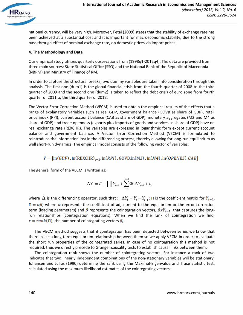
The Vector Error Correction Method (VECM) is used to obtain the empirical results of the effects that a range of explanatory variables such as real GDP, government balance (GOVB as share of GDP), retail price index (RPI), current account balance (CAB as share of GDP), monetary aggregates (M2 and M4 as share of GDP) and trade openness (exports plus imports of goods and services as share of GDP) have on real exchange rate (REXCHR). The variables are expressed in logarithmic form except current account balance and government balance. A Vector Error Correction Method (VECM) is formulated to reintroduce the information lost in the differencing process, thereby allowing for long-run equilibrium as well short-run dynamics. The empirical model consists of the following vector of variables:

The general form of the VECM is written as:

tit

p

i

itt YYY

1

1

1

where is the differencing operator, such that : 1 ttt YYY ; is the coefficient matrix for ,

, where represents the coefficient of adjustment to the equilibrium or the error correction term (loading parameters) and represents the cointegration vectors, that captures the long-run relationships (cointegration equations). When we find the rank of cointegration we find,

, the number of cointegrating vectors . The VECM method suggests that if cointegration has been detected between series we know that there exists a long-term equilibrium relationship between them so we apply VECM in order to evaluate the short run properties of the cointegrated series. In case of no cointegration this method is not required, thus we directly precede to Granger causality tests to establish causal links between them. The cointegration rank shows the number of cointegrating vectors. For instance a rank of two indicates that two linearly independent combinations of the non-stationary variables will be stationary. Johansen and Julius (1990) determine the rank using the Maximal-Eigenvalue and Trace statistic test, calculated using the maximum likelihood estimates of the cointegrating vectors.


ISSN: 2226-3624


5 Empirical Results

5.1. Time Series Properties of the Variables

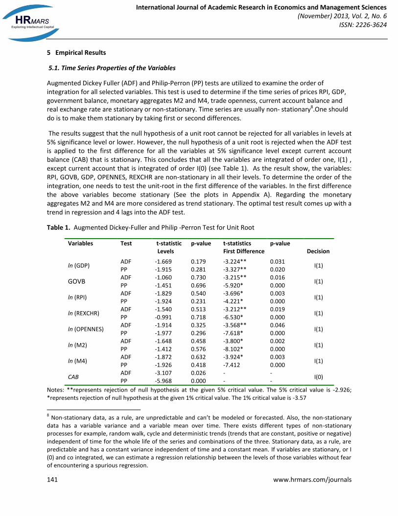
Augmented Dickey Fuller (ADF) and Philip-Perron (PP) tests are utilized to examine the order of integration for all selected variables. This test is used to determine if the time series of prices RPI, GDP, government balance, monetary aggregates M2 and M4, trade openness, current account balance and real exchange rate are stationary or non-stationary. Time series are usually non- stationary8.One should do is to make them stationary by taking first or second differences.

The results suggest that the null hypothesis of a unit root cannot be rejected for all variables in levels at 5% significance level or lower. However, the null hypothesis of a unit root is rejected when the ADF test is applied to the first difference for all the variables at 5% significance level except current account balance (CAB) that is stationary. This concludes that all the variables are integrated of order one, I(1) , except current account that is integrated of order I(0) (see Table 1). As the result show, the variables: RPI, GOVB, GDP, OPENNES, REXCHR are non-stationary in all their levels. To determine the order of the integration, one needs to test the unit-root in the first difference of the variables. In the first difference the above variables become stationary (See the plots in Appendix A). Regarding the monetary aggregates M2 and M4 are more considered as trend stationary. The optimal test result comes up with a trend in regression and 4 lags into the ADF test.

Table 1. Augmented Dickey-Fuller and Philip -Perron Test for Unit Root

Variables Test t-statistic p-value t-statistics p-value Levels First Difference Decision

ln (GDP) ADF -1.669 0.179 -3.224** 0.031

I(1) PP -1.915 0.281 -3.327** 0.020

GOVB ADF -1.060 0.730 -3.215** 0.016

I(1) PP -1.451 0.696 -5.920* 0.000

ln (RPI) ADF -1.829 0.540 -3.696* 0.003

I(1) PP -1.924 0.231 -4.221* 0.000

ln (REXCHR) ADF -1.540 0.513 -3.212** 0.019

I(1) PP -0.991 0.718 -6.530* 0.000

ln (OPENNES) ADF -1.914 0.325 -3.568** 0.046

I(1) PP -1.977 0.296 -7.618* 0.000

ln (M2) ADF -1.648 0.458 -3.800* 0.002

I(1) PP -1.412 0.576 -8.102* 0.000

ln (M4) ADF -1.872 0.632 -3.924* 0.003

I(1) PP -1.926 0.418 -7.412 0.000

CAB ADF -3.107 0.026 - -

I(0) PP -5.968 0.000 - -

Notes: **represents rejection of null hypothesis at the given 5% critical value. The 5% critical value is -2.926; *represents rejection of null hypothesis at the given 1% critical value. The 1% critical value is -3.57

8 Non-stationary data, as a rule, are unpredictable and can’t be modeled or forecasted. Also, the non-stationary

data has a variable variance and a variable mean over time. There exists different types of non-stationary processes for example, random walk, cycle and deterministic trends (trends that are constant, positive or negative) independent of time for the whole life of the series and combinations of the three. Stationary data, as a rule, are predictable and has a constant variance independent of time and a constant mean. If variables are stationary, or I (0) and co integrated, we can estimate a regression relationship between the levels of those variables without fear of encountering a spurious regression.


ISSN: 2226-3624


5.2 Testing for Co-integration

As a general rule, non-stationary time series variables should not be used in regression models in order to avoid the problem of spurious regression. However, Engle and Granger (1987) pointed out that a linear combination of two or more non-stationary series may be stationary. If such a stationary linear combination does exist, the non-stationary time series are said to be cointegrated and the stationary linear combination can be interpreted as a long run equilibrium relationship among the variables. Since all the variables are not stationary at levels according to ADF and PP results, it is necessary to carry out a cointegration test to investigate the long-run relationships among all those I(1) variables before conducting any further analysis on their long-run relationship.

Table 2 below presents the results of the cointegration tests based on Johansen’s (1991, 1996) maximum likelihood procedure test.

Table 2. Cointegration test results based on the Johansen maximum likelihood procedure

Eigenvalues H0 H1 5% critical value

Test values

Trace tests

0.5792 r = 0 r > 0 29.91 30.62*

0.4451 r ≤ 1 r > 1 26.73 19.67

0.3380 r ≤ 2 r > 2 19.31 14.89

0.3092 r ≤ 3 r > 3 18.56 13.44

0.2933 r ≤ 4 r > 4 14.98 10.91

0.1710 r ≤ 5 r > 5 11.92 8.93

0.1425 r ≤ 6 r > 6 9.24 5.67

0.0120 r ≤ 7 r > 7 7.79 3.76

tests

0.5792 r = 0 r = 1 28.34 29.19*

0.4451 r = 1 r = 2 23.96 18.12

0.3380 r = 2 r = 3 19.11 14.35

0.3092 r = 3 r = 4 14.56 13.44

0.2933 r = 4 r = 5 11.10 9.76

0.1710 r = 5 r = 6 9.12 7.43

0.1425 r = 6 r = 7 8.28 5.35

0.0120 r = 7 r = 8 7.79 3.76

Notes: * represents rejection of the null hypothesis at the given 5% critical value. is the maximal eigenvalue

test statistic for at most r cointegrating vectors against the alternative of r+1 cointegrating vectors. Trace is the stochastic matrix trace test statistic for at r cointegrating vectors.

Table 2 provides empirical support for a long run relationship between above mentioned variables since the null hypothesis of no cointegration is rejected. Both the trace tests and tests suggest that there is one cointegrating vector.


ISSN: 2226-3624


Table 3. The estimated cointegrating vector applying the Johansen procedure

Variables ∆ ln(EXCHR)

1.000 0.955413 1.94*** 0.054 0.062

∆ln (RPI) 0.022415 [0.099]***

-0.324476 -2.97** 0.129 0.191

∆ln (GDP) -0.044717 [0.123]

-0.299381 -1.64 0.197 0.136

∆ln (OPENNES) -0.003412 [0.175]

-0.936101 -1.42 0.223 0.277

∆ln (REXCHR)t-1 0.002730 [0.077]***

-0.129251 -1.22 0.325 0.451

∆ln (M2) -0.092881 [0.180]

-4.023441 -0.67 0.731 0.613

∆ln (M4) 0.633168 [0.459]

-3.927715 -0.98 0.591 0.622

∆CAB -0.009446 [0.157]

0.77295

1.41 0.102 0.477

∆ (GOVB) 0.001726 [0.092]***

0.955413 1.94*** 0.054 0.062

Dum1 -0.029912 [0.089]***

0.18231 1.91*** 0.074 0.062

Dum2 -0.008114 [0.171]

-0.11542 0.77 0.163 0.329

Notes: represents the cointegrating vector and represents the adjustment parameter vector; 1.000 implies

that the cointegrating vector is normalized with respect to the variable. Brackets denote probability value; **and *** represents rejection of the null hypothesis at the given 5% and10% critical value, respectively; z statistics is a test statistic for the alpha parameter and the p values are also probabilities for alpha .

The co-integrating vector is normalized with respect to the real exchange rate. The short run adjustment parameter alpha of the real exchange rate seems to be statistically insignificant. It should be pointed out that if the alpha parameter for a specific variable is not statistically significant it means that the variable is weakly exogenous. It is the case for all variables except government balance, RPI, real GDP and the dummy variable (Dum1) that reflects the effects of global financial crisis. This reveals that global financial crisis and the debt crisis of euro zone proved that structural shocks weigh down competiveness. The results of beta coefficients in (Table 3) indicate the long run relationship between real effective exchange rate and other macroeconomic variables. These results reveal that the long run determinants of the exchange rate are retail price index and government balance as only these variables are statistically significant in the long run. Real GDP, trade openness, current account, and monetary agregates are found to be statistically insignificant (see in Appendix B the impulse response functions).

It is clear that trade openness, current account and M2 basing on the alpha parameters do not explain the short run variations on the real effective exchange rate, meaning that these variables are weak exogenous. Also they are not affected by the long term co-integration relationship. For this reason we perform a Granger causality Wald test to investigate if causal links exist between exchange rate, trade openness, current account GDP and M2 variables.


ISSN: 2226-3624


5.3 A Causality Analysis According to Granger (1969), Y is said to “Granger-cause” X if and only if X is better predicted by using the past values of Y than by not doing so with the past values of X being used in either case. The following gives a clear picture about this:

(i) If a scalar Y can help to forecast another scalar X, then we say that Y Granger-causes X;

(ii) If Y causes X and X does not cause Y, it is said that unidirectional causality exists from Y to X;

(iii) If Y does not cause X and X does not cause Y, then X and Y are statistically independent; and

(iv) If Y causes X and X causes Y, it is said that feedback exists between X and Y.

Essentially, Granger‟ s definition of causality is framed in terms of predictability. With the regression analysis we want to estimate whether exchange rate determines the economic size (GDP) in Macedonia and whether GDP can encourage the level of exchange rate. Namely, we want to find out if the changes

in the level of exchange rate will respond with changes in the level of GDP. In order to test for direct causality between selected macroeconomic variables and exchange rate, we perform a Granger causality test using the following equations:

Where X and Y are the time series sequences, are the respective intercepts and are white

noise error terms and k is the maximum lag length used in each time series. The optimal lag length is determined using the Akaike’s information criteria, thus 4 lags are optimal for this set of data. The Granger Causality analysis is done for the real GDP, trade openness, current account and the monetary aggregate M2 in relation with the real effective exchange rate. The results are displayed in the Table 4 below.

Table 4. Granger Causality Wald Tests

Pairwise Granger Causality Tests Sample: 1998Q1- 2012Q4 Lags: 4 Null Hypothesis: Obs F-Statistic Prob. GDP does not Granger Cause REXCHER 58 2.40454 0.1622 REXCHER does not Granger Cause GDP 0.46655 0.7599 M2 does not Granger Cause REXCHER 58 1.20869 0.3191 REXCHER does not Granger Cause M2 1.59565 0.1904 OPENNESS does not Granger Cause REXCHER 58 1.16291 0.3387 REXCHER does not Granger Cause OPENNESS 1.13364 0.3517


ISSN: 2226-3624


M2 does not Granger Cause GDP 58 2.13105 0.0910 GDP does not Granger Cause M2 2.04451 0.1026 OPENNESS does not Granger Cause GDP 58 1.59458 0.1907 GDP does not Granger Cause OPENNESS 0.51534 0.7248 CAB does not Granger Cause REXCHR 58 0.93364 0.4523 REXCHR does not Granger Cause CAB 1.90706 0.1242 Author’s calculations

We regress the GDP on its own lagged values and on lagged values of exchange rate by generating tests for the null hypothesis. The estimated coefficients on the lagged values of exchange rate are jointly zero. The first test is a Wald test that the coefficients on the four lags of the exchange rate that appear in the equation of GDP are jointly zero. The null hypothesis that exchange rate does not Granger cause GDP cannot be rejected, meaning that the exchange rate does not augment the GDP, which means that if the exchange rate change, the GDP will not follow. The evidence of the causality of GDP related to exchange rate has the same effect, meaning that if GDP change the exchange rate will not follow. Therefore, we accept the null hypothesis which states that exchange rate does not Granger cause GDP. Based on the relationship we can conclude that exchange rate and GDP are statistically indipendent. This conclusion is partially consistent with these findings, (Fetai, 2011), (Besimi et al 2006 & 2009), (Krstevska et al 2003).

The second equation estimates the causality between exchange rate (REXCHR) and M2. Also the null hypothesis cannot be rejeceted meaning that if the exchange rate will change, M2 will not follow and vice-versa, so we can conclude that these two variables are also statistically indipendent. Thus, a devaluation of the Denar/Euro will have approximately zero effect on the monetary aggregate M2.

The third and sixth equations belong to the relationship between trade openness and exchange rate and current account and exchange rate, respectively. From the causality test is clear that for these equations the null hypothesis cannot be rejected for the both versions, meaning that trade openness does not granger cause exchange rate and current account does not Granger cause exchange rate and vice-versa.. A devaluation of the Denar/Euro will have zero effect on current account and exports and imports of goods and services (trade openness). This result is partially consistent with Jovanovic (2009). He claims that the exchange rate does not have significant effect on exports and imports. Imports are not price elastic, so the low and insignificant coefficient of import does not depend on the exchange rate. Particularly, imports depend on growth in consumption, investments and metal prices.

Considering the effects of the exchange rate over GDP, trade openness, and monetary aggregate M2, the empirical findings of VECM and the causality test suggest that Republic of Macedonia does not pay considerable costs in maintaining the fix exchange regime, since the exchange rate does not have significant effect on the above variables. From this study, we find out some relevant arguments that support the fix exchange regime: first, the poor performance of the balance of payments components, such as current account deficit, exports and imports do not rely on the exchange rate. Second, monetary aggregates and trade openness are defined inelastic to exchange rate. Third, with a fix exchange regime the Central Bank can control the degree of euroisation through following a restrictive monetary policy. And last but not least, the credibility towards national currency is much higher. This conclusion is consistent with the findings of Jovanovic (2007, 2009); Nenovski and Makrevska (2009).


ISSN: 2226-3624


6 Conclusion This study develops an empirical model to examine the long run and short run relationships between real exchange rate and a range of macroeconomic variables, such as real GDP, government fiscal balance, retail price index, trade openness, current account balance and monetary aggregates. The research further attempts to investigate the effects of the real exchange rate on selected macroeconomic variables using Granger Causality test. The findings of this study provide important results. Based on VECM results real GDP, trade openness, current account and monetary aggregates do not have significant effect on the real effective exchange rate in the short run as well as long run. Regarding the retail price index and government balance are significant in the short as well as long run dynamics. Also, based on the causality test was found that real exchange rate does not seem to cause GDP and likewise, GDP does not cause exchange rate. The similar result we obtained for current account, trade openness and monetary aggregate M2, meaning that these variables do not cause the exchange rate and likewise, exchange rate does not cause current account, trade openness and M2, respectively. It is evident that the nature of their relationship is influenced by other factors, such as euroization and structural shocks.

Thus, according to the empirical results, we found out relevant arguments that support the current regime i.e. fix regime of the exchange rate which ensures macroeconomic stability of the country. Taking into consideration the following characteristics euroisation, exchange rate pass through effect and credibility, introducing a float exchange regime is likely to induce more costs than benefits for the economy, as the global financial crisis of 2008 proved that still country face the lack of complete credibility of the national currency, monetary and fiscal policies. Moreover, countries like Macedonia with high level of euroisation and with high foreign denominated debt may not be able to afford sharp devaluation (more possible with a flexible regime) because that will increase the burden debt and other negative consequences in the economy.

References:

1. Belke.A. & Zenkić.A. (2006), ‘Exchange Rate Regimes and the Transition Process in the Western Balkans’, Berlin, Germany, pg. 21.

2. Besimi F. (2009), ‘Monetary and Exchange Rate Policy in Macedonia’, Accession to the European Union-Lambert Academic Publishing, Germany.

3. Bogoev J. (2006), ‘Central Bank Independence, Transparency and Accountability-The Case of South East Europe’, M.Sc. Dissertation at Staffordshire University, UK.

4. Cîtu F. (2003), ‘A VAR Investigation of the Transmission Mechanism in New Zealand’, Reserve Bank of New Zealand

5. Disyatat P. (2001), ‘Currency Crises and the Real Economy: The Role of Banks. IMF, Working Paper No. 01/49, Internationally Monetary Fund

6. Egert B. & Macdonald R. (2006), ‘Monetary Transmission Mechanism in Transition Economies: Surveying the Surveillance’, Magyar Nemzeti Bank, MNB Working Paper, No. 2006/5.

7. Engle, R. F.; Granger, C. W. J. (1987). Co-integration and error correction: representation, estimation, and testing. Econometrica , 55, 251-276

8. Fetai B. (2011), ‘Exchange Rate Pass-Through in Transition Economies: The Case of the Republic of Macedonia’, William Davidsion Institute, Working Paper Number 1014, University of Michigan.


ISSN: 2226-3624


9. Gosh, Atish R., Anne-Marie Gulde, Jonathan Ostry, and Holger Wolf, 1997, „Does the Nominal Exchange Rate Matter?“ NBER Working Paper No. 5874

10. Granger, C. (1969). Investigating Casual Relationship by Econometric Models and Cross Sprectal Methods. Econometrica , 37, 424-458.

11. Husain, A.,Mody, A. and Rogoff, K. (2004), Exchange rate regime durability and performance in developing versus advanced economies (IMF and Havard University).

12. Jovanovic B. (2007), ‘The Fundamental Equilibrium Exchange Rate of the Denar’ Unpublished Master’s thesis, Staffordshire University: UK..

13. Jovanovic B. (2009), ‘Should the Macedonian Denar be Devaluated? Some Evidence from the Trade Equations’, South-East Europe Review 3/2009.

14. Jurgen Von Hagen and Zhow, J. (2002). “The Choice of Exchange Rate Regime: An Empirical Analysis for Transition Economies” ZEI working paper Germany

15. Krstevska A., Terzijan S., Stojanova B. & Besimi F. (2003), ‘Transmission Effect of the Exchange Rate for Monetary Strategy of the NBRM’, National Bank of the Republic of Macedonia, Economic Research No.II/2003

16. Levy-Yeyati, E. and Sturzenegger, F. (2000), „Classifying Exchange Rate Regimes: Deeds vs. Words,“ mimeo, Universidad Torcuato Di Tella, Buenos Aires.

17. Markiewicz, A. (2006) “Choice of Exchange Rate Regime in Transition Economies: An Empirical Analysis” Journal of Comparative Economics 34 (2006) 484 – 498.

18. Mishkin Frederic S. (2001), ‘The Transmission Mechanism and the Role of Asset Prices in Monetary Policy’, Working Paper 8617, National Bureau of Economic Research, http://www.nber.org/papers/w8617

19. McKinnon, Ronald, (1963), „Optimum Currency Areas,“ American Economic Review 53 (September): 717--725

20. Melvin, M. (1985), ‘Choice of an Exchange Rate Regime and Macroeconomic Stability’, in Journal of Money, Credit and Banking, 17:468-78.

21. Moosa, I.A. 2005. “Exchange Rate Regimes: Fixed, Flexible or Something in Between?,” London: Palgrave

22. Mundell, Robert, 1961, „A Theory of Optimal Currency Areas,“ American Economic Review 51 (September): 657--665

23. NBRM, Annual Reports, Published March –April 2005-2010 24. Nenovski T. & Makrevska E.(2009), ‘Influence of the Economic Crisis on the Exchange Rates of

the Countries from Eastern and Central Europe’,Skopje 2009

http://www.nber.org/papers/w8617


ISSN: 2226-3624


Appendix A Plots of the first difference of the variables used in the empirical research

-16

-12

-8

-4

0

4

8

12

1998 2000 2002 2004 2006 2008 2010 2012

Differenced GDP

-16

-12

-8

-4

0

4

8

12

16

20

1998 2000 2002 2004 2006 2008 2010 2012

Differenced OPENNESS

-6

-5

-4

-3

-2

-1

0

1

2

3

1998 2000 2002 2004 2006 2008 2010 2012

Current account balance

-6

-4

-2

0

2

4

1998 2000 2002 2004 2006 2008 2010 2012

Differenced Government Balance

-8

-4

0

4

8

12

1998 2000 2002 2004 2006 2008 2010 2012

Differenced Real Effective Exchange Rate

-8

-4

0

4

8

12

16

1998 2000 2002 2004 2006 2008 2010 2012

Differenced M2


ISSN: 2226-3624


-8

-6

-4

-2

0

2

4

6

8

98 99 00 01 02 03 04 05 06 07 08 09 10

Differenced M4

-4

-2

0

2

4

6

8

1998 2000 2002 2004 2006 2008 2010

Differenced RPI

Appendix B

The effects of the exchange rate on GDP, trade openness and monetary aggregate M2

-1.0

-0.5

0.0

0.5

1.0

1.5

2.0

2.5

1 2 3 4 5 6 7 8 9 10

REXCHR GDP

OPENNESS M2

Response of REXCHR to Cholesky

One S.D. Innovations

-2

-1

0

1

2

3

4

1 2 3 4 5 6 7 8 9 10

REXCHR GDP

OPENNESS M2

Response of GDP to Cholesky


-2

0

2

4

6

8

1 2 3 4 5 6 7 8 9 10

REXCHR GDP

OPENNESS M2

Response of OPENNESS to Cholesky


-1.0

-0.5

0.0

0.5

1.0

1.5

2.0

1 2 3 4 5 6 7 8 9 10

REXCHR GDP

OPENNESS M2

Response of M2 to Cholesky


an empirical analysis of the exchange rate regime in the republic of...

Documents