an empirical comparison of methods for computing bayes factors

An Empirical Comparison of Methods forComputing Bayes Factors in Generalized

Linear Mixed Models

Sandip SINHARAY and Hal S STERN

Generalized linear mixed models (GLMM) are used in situations where a numberof characteristics (covariates) affect a nonnormal response variable and the responses arecorrelated due to the existence of clusters or groups For example the responses in biologicalapplications may be correlated due to common genetic factors or environmental factorsThe clustering or grouping is addressed by introducing cluster effects to the model theassociated parameters are often treated as random effects parameters In many applicationsthe magnitude of the variance components corresponding to one or more of the sets ofrandom effects parameters are of interest especially the point null hypothesis that one ormore of the variance components is zero A Bayesian approach to test the hypothesis is touse Bayes factors comparing the models with and without the random effects in questionmdashthis work reviews a number of approaches for estimating the Bayes factor We performa comparative study of the different approaches to compute Bayes factors for GLMMsby applying them to two different datasets The first example employs a probit regressionmodel with a single variance component to data from a natural selection study on turtlesThe second example uses a disease mapping model from epidemiology a Poisson regressionmodel with two variance components Bridge sampling and a recent improvement known aswarp bridge sampling importance sampling and Chibrsquos marginal likelihood calculation areall found to be effective The relative advantages of the different approaches are discussed

Key Words Bridge sampling Chibrsquos method Importance sampling Marginal densityReversible jump Markov chain Monte Carlo Warp bridge sampling

1 INTRODUCTION

Generalized linear mixed models (GLMMs) or generalized linear models with randomeffects are used in situations where a nonnormal response variable is related to a set ofpredictors and the responses are correlated due to the existence of groups or clusters The

Sandip Sinharay is Research Scientist Educational Testing Service MS-12T Rosedale Road Princeton NJ 08541(E-mail ssinharayetsorg) Hal S Stern is Professor and Chair Department of Statistics University of California4800 Berkeley Place Irvine CA 92697

ccopy2005 American Statistical Association Institute of Mathematical Statisticsand Interface Foundation of North America

Journal of Computational and Graphical Statistics Volume 14 Number 2 Pages 415ndash435DOI 101198106186005X47471

415

416 S SINHARAY AND H S STERN

groups or clusters are addressed by incorporating a set of random effects parameters in themodel In many applications the magnitude of the variance components corresponding toone or more of the sets of random effects are of interest especially the point null hypothesisthat the variance components in question are equal to zero A Bayesian approach for testinga hypothesis of this type is to compute the Bayes factor comparing the models suggested bythe null and the alternative hypotheses The primary objective of this work is to apply andevaluate the performance of different approaches for estimating the Bayes factor comparingthe GLMMs

A number of related studies exist in the statistical literature Albert and Chib (1997)provided a broad survey of the use of Bayes factors for judging a variety of assumptionsincluding assumptions regarding the variance components in conditionally independenthierarchical models (which include GLMMs as a special case) Han and Carlin (2001) pro-vided a review and empirical comparison of several Markov chain Monte Carlo (MCMC)methods for estimating Bayes factors emphasizing normal linear mixed model applica-tions Their study does not include importance sampling or warp bridge sampling PaulerWakefield and Kass (1999) provided a number of analytic approximations for comput-ing Bayes factors for variance component testing in linear mixed models DiCiccio KassRaftery and Wasserman (1997) compared several simulation-based approximation meth-ods for estimating Bayes factors Their study was quite general whereas the present workfocuses on GLMMs The present study adds to the literature by focussing on GLMMs (morespecifically on testing variance components in GLMMs) incorporating complex GLMMswith multiple variance components and incorporating new developments like warp bridgesampling (Meng and Schilling 2003) Our work should be of great interest to researchersworking with GLMMs but others will also find the results especially the findings on warpbridge sampling useful

Section 2 discusses a number of preliminary ideas regarding GLMMs Section 3 re-views the Bayes factor and approaches for estimating it Section 4 compares the differentapproaches in the context of a random effects probit regression model applied to data froma natural selection study (Janzen Tucker and Paukstis 2000) Section 5 takes up a morecomplex example a Poisson-normal regression model with spatial random effects and het-erogeneity random effects applied to Scotland lip-cancer data (Clayton and Kaldor 1987)Section 6 provides a discussion of our findings and recommendations

2 PRELIMINARIES

21 THE GENERALIZED LINEAR MIXED MODEL

In a GLMM observations y1 y2 yn are modeled as independent given canonicalparameters ξirsquos and a scale parameter φ with density

f(yi|ξi φ) = exp[yiξi minus a(ξi) + b(yi)]φ

EMPIRICAL COMPARISON OF METHODS FOR COMPUTING BAYES FACTORS 417

We take φ = 1 henceforth The two examples we consider in detail do not have a scaleparameter All of the methods described here can accommodate a scale parameter Letmicroi = E(yi|ξi) = aprime(ξi) The mean microi is expressed as a function of a predictor vector xptimes1

i a vector of coefficients αptimes1 and a random effects vector bqtimes1 through the link functiong(microi) = xprime

iα + zprimeib where zqtimes1

i is a design vector (typically 01) identifying the randomeffects Usually for a vector of unknown variance components θmtimes1 f(b|θ) is assumed tobe N (0D(θ)) where D(θ) is positive definite The magnitude of θ determines the degreeof over-dispersion and correlation among yirsquos Typically D(θ) = 0 iff θ = 0

22 LIKELIHOOD FOR GENERALIZED LINEAR MIXED MODELS

The likelihood function L(αθ|y) for a GLMM is given by

L(αθ|y) =int

b

nprod

i=1

f(yi|ξi)

f(b|θ)db =

intb

nprod

i=1

f(yi|αb)

f(b|θ)db middot (21)

The integral is analytically intractable making computations with GLMMs difficult Insimple problems as the one in Section 4 (where the model has a single random effectwith 31 levels) it is possible to use numerical integration Numerical integration techniques(eg Simpsonrsquos rule) or Laplace approximation (Tierney and Kadane 1986) are problematicfor high-dimensional b For the more elaborate example of Section 5 we use importancesampling to compute the likelihood (as in eg Geyer and Thompson 1992)

23 TESTING HYPOTHESES ABOUT VARIANCE COMPONENTS FOR GLMMS

Inferences about the contribution of the random effects to a GLMM are mostly obtainedby examining point (or interval) estimates of the variance parameters in D In many practicalproblems scientific investigators may like to test whether a particular variance componentis zero The classical approaches for testing in this context are the likelihood ratio test(LRT) using a simulation-based null distribution or the score test (Lin 1997) Our studyconcentrates on the Bayes factor a Bayesian tool to perform hypothesis testing or modelselection

3 BAYES FACTORS

31 INTRODUCTION

The Bayesian approach to test a hypothesis about the variance component(s) is tocompute the Bayes factor BF01 = p(y|M0)

p(y|M1) which compares the marginal densities (also

known as marginal likelihoods) of the data y under the two models M0 (one or more of thevariance components is zero) and M1 (variance unrestricted) suggested by the hypotheseswhere p(y|M) =

intp(y|ωM)p(ω|M)dω is the marginal density under model M and ω

denotes the parameters of model M Kass and Raftery (1995) provided a comprehensivereview of Bayes factors including information about their interpretation


The Bayes factor is also the ratio of posterior and prior odds

BF01 =p(M0|y)p(M1|y)

p(M0)p(M1)

(31)

This expression is useful in forming an estimate of the Bayes factor via reversible jumpMarkov chain Monte Carlo as described in the following

32 APPROACHES FOR ESTIMATING THE BAYES FACTOR

The key contribution of our work is to bring different computational methods to bear onthe problem of estimating the Bayes factor to test for the variance components for GLMMsFor these models the marginal densities required by the Bayes factor cannot be computedanalytically for either M1 or M0 For the remainder of this section ω = (αθ) implyingthat the random effects parameters b have been integrated out The final part of this sectiondiscusses an alternative parameterization

Different approaches exist for estimating the Bayes factor This work briefly reviews anumber of such approaches that have been applied in other models and then explores theiruse for GLMMs We will use the notation p(ω|yM) to denote the posterior density undermodel M and q(ω|yM) equiv p(y|ωM)p(ω|M) to denote the unnormalized posteriordensity

We consider the following approaches in our work (1) Importance sampling (seeeg DiCiccio et al 1997) (2) Markov chain Monte Carlo based calculation of the marginallikelihood (Chib 1995 Chib and Jeliazkov 2001) (3) bridge sampling and its enhancements(Meng and Wong 1996 Meng and Schilling 2003) and (4) reversible jump MCMC (Green1995) The methods are briefly reviewed later in this section The first three of the aboveapproaches estimate the marginal density of the data separately under each model the ratioof the estimated marginal densities giving the estimated Bayes factor Reversible jumpMCMC approaches estimate the Bayes factor directly

321 Importance Sampling

Importance sampling estimates of the marginal density are based on the identity

p(y|M) =int

p(y|ωM)p(ω|M)d(ω)

d(ω)dω

for any density function d() Then given a sampleωi i = 1 2 N from the ldquoimportancesampling distributionrdquo d() an estimate of the marginal density of the data under model Mis

p(y|M) asymp 1N

Nsumi=1

q(ωi|yM)d(ωi)

The choice of importance sampling density is crucial the density d() must have tails asheavy as the posterior distribution to provide reliable estimates of the marginal likelihood


Common choices are normal or t-distributions with suitable location and scale We discussthe choice of importance sampling density further in the section that discusses warp bridgesampling (Meng and Schilling 2003)

322 Chibrsquos Method

Chib (1995) suggested estimating p(y|M) by estimating at any ω = ωlowast the right handside of

p(y|M) =p(y|ωM)p(ω|M)

p(ω|yM)middot (32)

The computation of p(y|ωlowastM) and p(ωlowast|M) are straightforward Given a sample from theposterior distribution kernel density approximation may be used to estimate the posteriorordinate p(ωlowast|yM) for low-dimensional ωlowast Alternatively Chib (1995) and Chib andJeliazkov (2001) gave efficient algorithms to estimate the posterior ordinate when Gibbssampling Metropolis-Hastings or both algorithms are used to generate a sample from theposterior distribution A number of points pertain specifically to the use of Chibrsquos methodsfor GLMMs

A key to using Chibrsquos method is doing efficient blocking of the parameters For mostGLMMs partitioningω into two blocks one containing the fixed effects parameters and theother containing the variance parameters is convenient For a few simple GLMMs Gibbssampling can be used to generate from the posterior distribution and the marginal densityevaluated using the approach of Chib (1995) However some Metropolis steps are generallyrequired with GLMMs necessitating the use of the Chib and Jeliazkov (2001) algorithm

For increased efficiency of estimation ωlowast in (32) is generally taken to be a highdensity point in the support of the posterior distribution Popular choices of ωlowast include theposterior mean or posterior median For GLMMs the posterior distribution of the varianceparameter(s) is skewed hence the posterior mode will probably be a better choice of ωlowast

323 Bridge Sampling

Meng and Wong (1996) described the use of bridge sampling for computing the ratioof normalizing constants when (1) there are two densities each known up to a normalizingconstant and (2) we have draws available from each of the two densities Though bridgesampling can sometimes be used to directly compute the BF (as a ratio of two normalizingconstants) it may be difficult to do so when the two models contain parameters that are notdirectly comparable or of different dimension Instead we use bridge sampling to computethe normalizing constant for a single density by choosing a convenient second density (withknown normalizing constant one) Let r = p(y|M) be the normalizing constant for theposterior distribution under model M (which is the marginal density or marginal likelihoodneeded for our Bayes factor calculations) Bridge sampling is based on the identity

r =intq(ω|yM)α(ω)d(ω)dωintα(ω)d(ω)p(ω|yM)dω

(33)


for any probability density d() and any function α() satisfying fairly general conditionsgiven by Meng and Wong (1996) Then if we have a sample ωi i = 1 2 n1 from theposterior distribution and a sample ωj j = 1 2 n2 from d the Meng-Wong bridgeestimator of r is

r asymp1n2

sumn2

j=1 q(ωj |yM)α(ωj)1n1

sumn1

j=1 d(ωj)α(ωj)middot

Meng and Wong showed that if the draws are independent the optimal choice of α(for minimizing the asymptotic variance of the logarithm of the estimate of r) for a given dis proportional to n1q(ω|yM) + n2rd(ω)minus1 which depends on the unknown r Theypropose an iterative sequence to estimate r

r(t+1) =1n2

n2sumj=1

l2j

s1l2j + s2r(t)

1n1

n1sumj=1

1s1l1j + s2r(t)

(34)

where sk = nk

n1+n2 k = 1 2 l1j = q(ωj |yM)d(ωj) and l2j = q(ωj |yM)d(ωj)

Starting with 1r(0) = 0 yields r(1) = 1n2

sumn2

j=1q(ωωωj |yM)

d(ωωωj) which is the importance sam-

pling estimate with importance density d() Also starting the sequence with r(0) = 0results in the reciprocal importance sampling (DiCiccio et al 1997) estimate after the firstiteration Meng and Schilling (2003) also showed how Chibrsquos method can be derived usingbridge sampling

The choice of α given above is no longer optimal if the draws are not independent(they are not generally independent for MCMC) Meng and Schilling (2003) recommendedadjusting the definition of α in that situation by using in it the effective sample sizesni = ni(1 minus ρi)(1 + ρi) where ρi is an estimate of the first-order autocorrelation for thedraws from the posterior or d respectively

We apply bridge sampling with d equiv N (0 I) or d equiv t(0 I) to obtain the marginallikelihoods Before doing so however we make use of a relatively new idea warp bridgesampling (Meng and Schilling 2003) Meng and Schilling (2003) showed that applying (33)after transforming the posterior density to match the first few moments of an appropriate d(eg a N (0 I) density) a transformation which does not change the normalizing constantresults in a more precise estimate of the marginal density They refer to their transformationas ldquowarprdquo-ing the density A Warp-I transformation would shift the posterior density tohave location zero this was proposed by Voter (1985) in physics Matching the mean andvariance (or related quantities like the mode and curvature) that is applying (33) with|S| q(micro minus Sω|yM) in place of q(ω|yM) for suitable choices of micro and S is a Warp-II transformation Matching the mean (mode) variance (curvature) and skewness that isapplying (33) with |S|

2 [q(micro minus Sω|yM) + q(micro + Sω|yM)] in place of q(ω|yM) is aWarp-III transformation

Application of warp bridge sampling does not require more computational effort thanordinary bridge sampling We only need draws from the posterior density and the importancedensity For Warp-II (34) is applied with l1j and l2j replaced by

l1j = |S|q(ωj |yM)d(Sminus1(ωj minus micro)) and l2j = |S|q(micro+ Sωj |yM)d(ωj)


For Warp-III the corresponding expressions are

l1j =|S|2

[q(ωj |yM) + q(2microminus ωj |yM)]d(Sminus1(ωj minus micro))

and

l2j =|S|2

[q(microminus Sωj |yM) + q(micro+ Sωj |yM)]d(ωj)middot

Meng and Schilling (2003) suggested analytical and empirical ways of finding optimal val-ues ofmicro and S to use in warp bridge sampling For example for the Warp-III transformationoptimal values can be found by maximizing over micro and S the quantity

sumj

radic1

φ(ωj)|S| (q(microminus Sωj |yM) + q(micro+ Sωj |yM)

)

for a sample ωj j = 1 2 n from a N (0 I) distribution where φ() denotes the multi-variate normal density Empirical studies suggest good estimates of r even for suboptimalchoices of the warping transformation (eg using sample moments rather than optimizingover micro and S)

Note that it is also possible to use the idea of warping transformations to developimportance sampling methods In other words one can choose the importance samplingdensity as N (0 I) and then transform the posterior distribution (with Warp-II or Warp-IIItransformations) before applying importance sampling

324 Reversible Jump MCMC

A very different approach for computing Bayes factor estimates requires constructingan ldquoextendedrdquo model in which the model index is a parameter as well The reversiblejump MCMC method suggested by Green (1995) samples from the expanded posteriordistribution This method generates a Markov chain that can move between models withparameter spaces of different dimensions Let πj be the prior probability on model j j =0 1 J The method proceeds as follows

1 Let the current state of the chain be (jωj)ωj=nj-dimensional parameter for modelj

2 Propose a new model jprime with probability h(j jprime) wheresum

jprime h(j jprime) = 13 a If jprime = j then perform an MCMC iteration within model j Go to Step 1

b If jprime = j then generate u from a proposal density qjjprime(u|ωj j jprime) and set

(ωjprime uprime) = gjjprime(ωj u) where g is a 1-1 onto function nj + dim(u) = njprime +dim(uprime)

4 Accept the move from j to jprime with probability

min

1p(y|ωjprime M = jprime)p(ωjprime |M = jprime)πjprimeh(jprime j)qjprimej(uprime|ωjprime jprime j)p(y|ωj M = j)p(ωj |M = j)πjh(j jprime)qjjprime(u|ωj j jprime)

∣∣∣∣partg(ωj u)part(ωj u)

∣∣∣∣


Step 3b is known as the dimension-matching step in which auxiliary random variables areintroduced (as needed) to equate the dimension of the parameter space for models j and jprimeIf the above Markov chain runs sufficiently long then p(Mj |y)p(M prime

j |y) asymp NjNjprime whereNj is the number of times the Markov chain reaches model j Therefore the Bayes factor

BFjjprimefor comparing models j and jprime can be estimated using (31) as BFjjprime asymp Nj

Njprime

πj

πjprime middot

325 Other Methods

The methods described here do not exhaust all possible methods Although our goalis to try and provide general advice the best approach for any specific application may befound outside our list The methods summarized in this work represent the set that we havefound most applicable to GLMMs We have omitted Laplacersquos method (see eg Tierneyand Kadane 1986) a useful approximation in many problems but increasingly unreliableas the number of random effects parameters increase in the GLMMs (Sinharay 2001) Theapproach of Verdinelli and Wasserman (1995) for nested models works well in our firstexample but requires density estimation and thus is less practical in higher dimensionalsettings like our second example (Sinharay and Stern 2003 Sinharay 2001) Other methodsfor computing Bayes factors which can be used in the context of GLMMs include theratio importance sampling approach by Chen and Shao (1997) path sampling (Gelman andMeng 1998) and product space search (Carlin and Chib 1995) Han and Carlin (2001) findmethods based on the idea of creating a product space (that is a space that encompasses theparameter space of each model under consideration) problematic for models where randomeffects cannot be analytically integrated out from the likelihood which is typically the casewith the GLMMs

33 PARAMETERIZATION

A number of the methods for estimating Bayes factors require computing the GLMMlikelihood p(y|ωM) for one or more values ofω If the accurate computation of p(y|ωM)which involves integrating out the random effects is time-consuming some of the methodsbecome impractical This especially affects those like importance sampling and bridgesampling that require more than one marginal likelihood computation Chibrsquos method ismore likely to succeed in such cases

One approach for circumventing this difficulty is to consider applying our variousapproaches with ω = (bαθ) rather than assuming that b has been integrated out Chib(1995) suggested this idea in the context of his approach and it applies more generally tothe other methods considered here For this choice of ω the marginal density p(y|M) forthe GLMM is

p(y) =int int

p(y|αθ)p(αθ)dαdθ

=int int int

p(y|αb)p(b|θ)p(αθ)dbdαdθ


Figure 1 Scatterplot with the clutches sorted by average birthweight

The advantage of the expanded definition of ω is that the computation of the likelihoodfunction p(y|ω) = p(y|αbθ) = p(y|αb) is straightforward However as a price topay for this simplification of the likelihood the dimension of the parameter space increasesby the number of components in b which is usually high even for simple GLMMs

4 EXAMPLE A NATURAL SELECTION STUDY

41 THE DATA AND THE MODEL FITTED

A study of survival among turtles (Janzen et al 2000) provides an example where aGLMM is appropriate The data consist of information about the clutch (family) mem-bership survival and birth-weight of 244 newborn turtles The scientific objectives are toassess the effect of birth-weight on survival and to determine whether there is any clutcheffect on survival Figure 1 shows a scatterplot of the birthweights versus clutch numberwith survival status indicated by the plotting character ldquo0rdquo if the animal survived and ldquoxrdquo ifthe animal died The clutches are numbered in increasing order of the average birthweightof the turtles in the clutch The figure suggests that the heaviest turtles tend to survive andthe lightest ones tend to die Some variability in the survival rates across clutches is evidentfrom the figure

Let yij denote the response (indicator of survival) and xij the birthweight of the jthturtle in the ith clutch i = 1 2 m = 31 j = 1 2 ni The probit regression modelwith random effects fit to the dataset is given by

bull yij |pij sim Ber(pij) where pij = Φ(α0 + α1xij + bi) i = 1 2 m = 31 j =1 2 ni

bull bi|σ2 iidsim N (0 σ2) i = 1 2 m

The birsquos are random effects for clutch (family) There is no clutch effect iff σ2 = 0


42 ESTIMATING THE BAYES FACTOR

The marginal likelihoods under the null model (M0) and full model (M1) are

p(y|M0) =int

p(y|αb = 0)p(α)dα

and

p(y|M1) =int

p(y|αb)p(b|σ2)p(α)p(σ2)dbdαdσ2

Our work uses the shrinkage prior distribution (see eg Daniels 1999) for the variancecomponents p(σ2) = c

(c+σ2)2 where c is the median of p(σ2) We fix c at 1 We setp(α) = N2(0 10 I)

Each of the methods (except reversible jump MCMC) requires that we evaluate thelikelihood p(y|α σ2) (ie we must integrate out b in the full model) For this relativelysmall problem we do so using Simpsonrsquos rule to perform the needed numerical integrationThe methods also require samples from the posterior distribution p(α σ2|y) This is doneusing an MCMC algorithm There is significant autocorrelation in the Markov chain andthe Gelman-Rubin convergence diagnostic (see eg Gelman et al 2003) suggests thatusing five chains of 1000 iterations after burn-ins of 200 iterations is sufficient to providea summary of the posterior distribution This results in a final posterior sample size of5000 Therefore all simulation-based estimates use posterior samples of size 5000 foreach model

The posterior mode and the information matrix at the mode which are used in someof the methods are found using the Newton-Raphson method The posterior mean andvariance required by some methods are computed from a preliminary MCMC run Forimportance sampling and bridge sampling we transform the variance to log(σ2) in theposterior distribution to improve the similarity of the normal (or t) importance samplingdensity Additional details concerning the implementation of the individual approachesfollow


The conditional distribution of σ2 is not of known form necessitating the use of theMetropolis algorithm for sampling from the joint posterior distribution of the parametersunder the mixed model The use of data augmentation by incorporating latent normal vari-ables in the probit model (Albert and Chib 1993) allows the use of Gibbs sampling for thefixed effects but did not improve the precision here The Metropolis algorithm is also usedto generate a sample from the null model

422 Importance and Bridge Sampling

We tried several variations of bridge and importance sampling We apply Warp-IItransformations with (1) posterior mode and square root of the curvature matrix as micro andS respectively (mode-curvature matching) and (2) posterior mean and a square root of the


posterior variance matrix as micro and S (mean-variance matching) The use of d equiv t4(0 I)resulted in more precise Bayes factor estimates than d equiv N (0 I) probably because theformer has more overlap than the latter with the skewed transformed posterior Thus wereport only the results for the t importance sampling or bridge sampling density It typicallytook three or four iterations for the bridge sampling iterative process to reach convergenceRecall that the first iteration of bridge sampling with sampling distribution d yields theimportance sampling estimate that corresponds to using d as importance sampling densityfor the transformed posterior

We also apply Warp-III transformations with mode-variance matching mean-variancematching and mode-curvature matching In this case d equiv t4(0 I) does not result in im-proved estimates relative to d equiv N (0 I) probably because after accounting for skewnessthe posterior distribution has been transformed into a distribution well-approximated by anormal distribution

Because there exists a significant autocorrelation in the posterior sample (eg first-order autocorrelations are in the range 8ndash9 for most parameters in the alternative model)we adjustα using the effective sample size approach for both Warp-II and Warp-III taking ρto be the sample lag-1 autocorrelation of 1(l1j + r) as in Meng and Schilling (2003) Thisadjustment requiring only a few lines of additional computer coding results in a significantincrease in precision


Using the notation from Section 324 we seth(j jprime) = πj = 5 forall j jprime Here parametervectors under the two models are ω0 = α and ω1 = (α σ2) When we try to move frommodel 0 to model 1 there is an increase in dimension as model 1 has a variance componentwhile model 0 does not We use the current value of α in model 0 as candidate value of αin model 1 and generate a candidate value of σ2 from an inverse gamma distribution withmean and variance as the posterior mode and curvature of σ2 under model 1 These choicesamount to using notations from Section 324 u = σ2 uprime = 0 g(x) = x and q(σ2) equiv theabove-mentioned inverse gamma distribution When we try to move from model 1 to model0 there is a reduction in dimension Therefore in generating candidate values under model0 we ignore the variance component for model 1 and use the current value ofα in model 1as candidate value of α under model 0 These amount to u = 0 uprime = σ2 and g(x) = x Tomove within a model we take a Metropolis step with a random walk proposal distribution

43 RESULTS

Numerical integration over all parameters provides us the true value of the Bayes factorof interest although the program takes about 62 hours of CPU time to run on an Alpha station500 workstation equipped with 400MHz 64-bit CPU and a gigabyte of RAM The true valueof the Bayes factor up to three decimal places is 1273

To learn about the precision of the different estimation approaches we compute the BF


Table 1 Estimates of the Bayes factor (along with their standard deviations and time taken to run theprogram) for the Turtles Dataset

Method Bayes factor estimate Std dev CPU time (min)

True value 1273 ndash ndash

Bridge Warp-III (optimal micro-curvature) 1273 0059 203Bridge Warp-III (mode-curvature) 1273 0063 203Bridge Warp-III (mode-variance) 1273 0076 203

Imp samp (Warp-III optimal micro-curvature) 1275 0066 80Imp samp (Warp-III mode-curvature) 1274 0068 80Imp samp (Warp-III mode-variance) 1275 0086 80

Bridge Warp-II (mean-variance) 1273 0094 131Bridge Warp-II (mode-curvature) 1274 0145 132

Imp samp Warp-II (mean-variance) 1272 0108 60Imp samp Warp-II (mode-curvature) 1274 0156 62

Chibrsquos (at mode) 1275 0492 161Chibrsquos (at mean) 1266 0724 160

RJ MCMC 1302 2032 180

a number of times with different random seeds Table 1 summarizes the mean and standarddeviation (sd) of 100 Bayes factor estimates obtained by the various methods The use of100 trials allows us to have confidence in the reported standard deviations (according totraditional sampling theory the reported standard deviations are accurate to within 15)Also shown in the table are the CPU times required for one computation of the Bayes factorestimate by each of the methods on the above-mentioned workstation

Table 1 indicates that all of the methods are effective with reversible jump Markovchain Monte Carlo having a much larger standard deviation We next discuss the results forimportance and bridge sampling The Warp-III transformation results in very efficient esti-mates (for both bridge sampling and importance sampling) even without the optimal choiceof micro and S Bridge sampling with Warp-III (using the effective sample size in computationof α()) is more efficient for this example than Warp-III importance sampling Runningbridge sampling to convergence reduces the standard error by about 10 relative to stop-ping after the first iteration (which is importance sampling) Warp-II bridge sampling andWarp-II importance sampling perform respectably as well especially for mean-variancematching Again bridge sampling seems to be more precise than importance samplingFigure 2 showing contour plots for the two-dimensional marginal posterior distributions(obtained using S-Plus functions ldquokderdquo and ldquocontourrdquo) demonstrates the effect of warpingon the posterior distribution The application of the Warp-III transformation takes the orig-inally nonnormal two-dimensional posteriors (the top row) into ones quite close to N (0 I)(the bottom row) Therefore it is no surprise that Warp-III provides such precise estimates

Chibrsquos method provides good results as well The standard deviation is larger thanfor the bridge and warp sampling Chibrsquos method does however have one advantage overimportance and bridge sampling in that it does not require that a matching or importance


Figure 2 Effect of warping on posterior distributions for the turtles data The first row shows the three bivariatemarginal posterior distributions for the original untransformed posterior distribution (showing the highly non-normal nature) The second row shows the effect of the Warp-II (mean-variance matching) transformation aftertaking the logarithm of σ2 The third row is for the Warp-III transformation with mode-curvature matching

sampling density be selected If the posterior distribution has features like an unusuallylong tail not addressed by our warping transformations then it is possible that the standarddeviation of importance and bridge sampling may be underestimated

A second factor in comparing the computational methods is the amount of compu-tational time required This has two dimensions the amount of time required to run theprogram and the time required to write the program The relative importance of these twodimensions depends on a userrsquos contextmdashif one will frequently analyze data using the samemodel then programming time is less important

Programming time of course depends on the programmer Our experience was that im-portance sampling (with transformations) takes considerably less time than bridge samplingto program Chibrsquos method builds on the existing MCMC code (required by all methods)however to us modifying it to compute the Bayes factor was more time consuming thandeveloping importance sampling methods The programming time for Chibrsquos method iscomparable to that for warp bridge sampling

Naturally the run time for importance sampling is less than that of bridge sampling Inthe present case the added precision of bridge sampling may not be worth the extra timeImportance sampling was also faster than Chibrsquos method but there are several mitigatingfactors that affect that comparison Importance (and bridge) sampling requires extensive


Table 2 Part of the Scotland Lip Cancer Dataset

County y p (in rsquo000) AFF E Neighbors

1 9 28 16 138 4 5 9 11 192 39 231 16 866 2 7 103 11 83 10 304 2 6 124 9 52 24 253 3 18 20 28

54 1 247 1 703 5 34 38 49 51 5255 0 103 16 416 5 18 20 24 27 5656 0 39 10 176 6 18 24 30 33 45 55

calculations of the likelihood function in problems where that is more complicated the timeadvantage of importance sampling will dissipate Also more efficient MCMC algorithmsmight make Chibrsquos method more competitive on speed Although all methods work wellhere our preference is for warp-transformed importance sampling for these data based onspeed and efficiency

5 EXAMPLE SCOTLAND LIP CANCER DATA

This section considers a more complex example with more than one variance compo-nent The computations become much more difficult and time-consuming for such models

51 DESCRIPTION OF THE DATASET

Table 2 shows a part of a frequently analyzed dataset (see eg Clayton and Kaldor1987) regarding lip cancer data in the 56 administrative districts in Scotland from 1975ndash1980 The objective of the original study was to find any pattern of regional variation in thedisease incidence of lip cancer The dataset contains yi pi EiAFFi Ni i = 1 2 56where for district i yi is the observed number of lip cancer cases among males from 1975ndash1980 pi is the population at risk of lip cancer (in thousands) Ei is the expected number ofcases adjusted for the age distribution AFFi is the percent of people employed in agricultureforestry and fishing (these people working outdoors may be under greater risk of the diseasebecause of increased exposure to sunlight) and Ni is the set of neighboring districts

52 A POISSON-GAUSSIAN HIERARCHICAL MODEL

The yirsquos are assumed to follow independent Poisson distributions yi|λi simPoisson(λiEi) i = 1 2 n where λi is a relative risk parameter describing risk af-ter adjusting for the factors used to calculate Ei As in Besag York and Mollie (1991)we use a mixed linear model for log(λ) log(λ) = Xβ + η + ψ where X is the covari-ate matrix β = (β0 β1)prime is a vector of fixed effects η = (η1 η2 ηn)prime is a vector ofspatially correlated random effects and ψ = (ψ1 ψ2 ψn)prime is a vector of uncorrelatedheterogeneity random effects


For known matrices C and diagonal M we take the prior distribution forη as a Gaussianconditional autoregressive (CAR) distribution that is η|τ 2 φ sim N (0 τ 2(IminusφC)minus1M) asin Cressie Stern and Wright (2000) where τ 2 andφ are parameters of the prior distributionThe parameter φ measures the strength of spatial dependence 0 lt φ lt φmax where φ = 0implies no spatial association andφmax is determined by the choice of C and M The elements

of the matrices C and M used here are mii = Eminus1i and cij =

(Ej

Ei

) 12I[jisinNi] where I[A]

is the indicator for event A For these choices of C and M φmax = 1752The ψrsquos are modeled as ψ|σ2 sim N (0 σ2D) where D is a diagonal matrix with dii =

Eminus1i and σ2 is a variance parameter In practice it appears often to be the case that eitherη or ψ dominates the other but which one will not usually be known in advance (Besag etal 1991)

The model above contains three covariance matrix parameters (τ 2 σ2 and φ) and 112random effects parameters making it a more challenging data set to handle computationallythan the turtle dataset The joint maximum likelihood estimate of ξ = (β0 β1 φ τ

2 σ2)prime

is ξMLE = (minus489 059 167 1640 0)prime The fifth component of the posterior mode is 0 aswell

53 ESTIMATING THE BAYES FACTORS

Because of the presence of more than one variance component in the model severalBayes factors are of interest These correspond to comparing any two of the four possiblemodels

bull ldquofull modelrdquo with σ2 and τ 2 (and φ)bull ldquospatial modelrdquo with τ 2 only as a variance component (also includes φ)bull ldquoheterogeneity modelrdquo with σ2 only as a variance componentbull ldquonull modelrdquo with no variance component

We focus on the three Bayes factors obtained by comparing any one of the three reducedmodels to the full model Any other Bayes factor of interest here can be obtained from thesethree

Using a transformation ν = η + ψ the likelihood for the full model (with randomeffects integrated out) L(β φ τ 2 σ2|y) can be expressed as

L(β φ τ 2 σ2|y) propint

nprodi=1

exp(minusEie

xprimeiβββ+νi

)eyi(xprime

iβββ+νi)

1|V|12

middot exp

minus1

2νprimeVminus1ν

dν

where V = τ 2(I minus φC)minus1M + σ2D To estimate the likelihood we use importance sam-pling (Section 321) with a t4 importance sampling distribution Note that the Warp bridgesampling method could be used here as well The mean and variance of the importancesampling distribution are the corresponding moments of ν = η+ψ computed from a pos-terior sample drawn from the conditional posterior distribution of (ηψ) given β φ τ 2 σ2


This procedure estimates the likelihood with reasonable precision within reasonable timeWe assume independent prior distributions β sim N2(0 20I) p(φ) =

Uniform(0 φmax) p(σ2) = 1(1+σ2)2 p(τ 2) = 1

(1+τ 2)2 middot Posterior samples are obtainedusing a Metropolis-Hastings algorithm The large number of parameters result in high au-tocorrelations and hence we use 5 chains of 10000 iterations of the MCMC after a burn-inof 2000 each (enough to achieve convergence according to the Gelman-Rubin convergencecriterion) Additional details about specific methods follow


Each of the conditional posterior distributions is sampled from using a Metropolis stepand thus the Chib and Jeliazkov (2001) approach is required As for the fixed point at whichthe posterior density is evaluated we use the sample mean of the posterior sample ratherthan the posterior mode because the latter is on the boundary of the parameter space andone of the terms required by Chibrsquos method is not defined there

532 Bridge and Importance Sampling

We apply Warp-II transformations with d equiv t4(0 I) and Warp-III transformationswith d equiv N (0 I) In both cases we use the sample mean and variance of the posteriorsample as the location and scale parameters of the transformation It may be possible to dobetter by optimizing over micro and S but the efficiency achieved by the mean-variance choicewas sufficient As in the turtle example because of strong dependence of the draws we usethe effective sample size (rather than the actual MCMC sample size) in the bridge samplingiteration

54 REVERSIBLE JUMP MCMC

It is possible in principle to compute all the Bayes factors from one reversible jumpMCMC that allows jumps among the four models We use three separate programs tocompute the three Bayes factors (and even then had trouble getting this approach to workwell) We set h(j jprime) = πj = 5 forall j jprime When we try to move from model j to model jprimewe generate auxiliary variable u to correspond to all of the parameters of model jprime that iswe do not retain values of the parameters from model j that are in model jprime as well Thiswas the approach of Han and Carlin (2001) as well For example when we try to movefrom the ldquofull modelrdquo to the ldquospatial modelrdquo we generate u from a 59-dimensional normalindependence proposal density whose mean and variance are determined by an earlier runof the MCMC algorithm for the ldquospatial modelrdquo The reasoning is that it would not beappropriate to just zero out the heterogeneity random effects because the remaining spatialeffects are not likely to represent the posterior distribution under the spatial model It wasdifficult to obtain reliable results from reversible jump MCMC apparently because of thelarge number of random effects which cannot be integrated out from the likelihood Han andCarlin (2001) found similar results As we show below the Bayes factor for comparing the


Table 3 Estimates of Bayes Factors (along with their standard deviations and time taken to run theprogram) for the Scotland Lip Cancer Dataset

Comparing Method Estimated BF Std dev CPU time(min)

ldquospatial True value 142 ndash ndashmodelrdquo Bridge W-III (mean-variance) 142 029 883

vs Imp samp W-III (mean-variance) 141 032 452ldquofull Bridge W-II (mean-variance) 143 040 652

modelrdquo Imp samp W-II (mean-variance) 144 065 305Chibrsquos (at mean) 144 132 811

RJMCMC 121 265 499

ldquoheterogen True value 066 ndash ndashmodelrdquo Bridge W-III (mean-variance) 066 0017 663



RJMCMC 032 182 309

ldquonull True value 115 times 10minus23 ndash ndashmodelrdquo Bridge W-III (mean-variance) 115 times 10minus23 152times 10minus25 554

vs Imp samp W-III (mean-variance) 115 times 10minus23 166 times 10minus25 282ldquofull Bridge W-II (mean-variance) 114 times 10minus23 266 times 10minus25 372

modelrdquo Imp samp W-II (mean-variance) 116 times 10minus23 364 times 10minus25 182Chibrsquos (at mean) 121 times 10minus23 146 times 10minus24 481

ldquofull modelrdquo to the ldquoheterogeneity modelrdquo or the ldquospatial modelrdquo could not be estimated to areasonable degree of accuracy even after trying a variety of Metropolis proposal densitiesThe Bayes factor favoring the ldquofullrdquo model over the ldquonullrdquo model is so large that we werenever able to accept a single step to the null model for any of our proposal densities

55 RESULTS

We use the importance sampling method with sample size one million to compute theldquotrue valuerdquo of the three Bayes factors Examining the variability of the importance ratiosfor the sampled one million points we conclude that the Bayes factor is determined up toa standard error of about 5 for the Bayes factor comparing the spatial model to the fullmodel and about 25 for the other two Bayes factors Warp-III bridge sampling with asample size of half million results in the same values These values serve as the true Bayesfactors for comparing the methods

Table 3 shows the average and standard deviation of 100 Bayes factors (with differentrandom seeds) obtained using each method and the CPU time taken for one computationof the Bayes factor estimate by each of these methods on the workstation mentioned in theprevious example The results here are completely consistent with those of the first exampleWarp bridge sampling importance sampling and Chibrsquos marginal likelihood approach yieldgood estimates The reversible jump MCMC approach performs unsatisfactorily even afterconsiderable tuning The standard deviation of the Bayes factor estimate is much smallerfor the Warp-III bridge sampling and importance sampling than the other methods Figure 3


Figure 3 Effect of warping on posterior distributions for the lip cancer data The first row shows four bivariatemarginal posterior distributions for the original untransformed joint posterior distribution (showing the highlynon-normal nature) The second row shows the effect of the Warp-II (mean-variance matching) transformationThe third row is for the Warp-III (mean-variance matching) transformation

shows how the warp transformations work in this higher dimensional problem by examiningcontour plots for some two-dimensional marginal posterior distributions

Han and Carlin (2001 p 1131) suggested that Chibrsquos method might not be effective inspatial models using Markov random field priors Our results indicate that it does provideacceptable Bayes factor estimates although as Han and Carlin pointed out one is required tosample the random effects individually which may become prohibitive in larger applications

6 DISCUSSION AND RECOMMENDATIONS

GLMMs are applied extensively and their use is likely to increase with the widespreadavailability of fast computational facilities and the increased sophistication of data analystsin a variety of disciplines In many applications of these models question arises about thenecessity of the variance components in the model One way to answer the question in factour preferred way is to examine the estimates of the variance components under the fullmodel This article arose as a result of several problems in which formal model comparisonswere desired by scientific investigators The objective of this study is to learn more aboutthe performance of different methods for computing the relevant Bayes factor estimates

The computation of the likelihood p(y|ωM) (averaging over the random effects) is


a nontrivial task for GLMMs If the model is simple and the dataset is small it is possibleto apply numerical integration For larger problems importance sampling is a possibleapproach (Geyer and Thompson 1992) our work finds that importance sampling with a t4sampling distribution works well

The computation of the Bayes factor involves integrating over the parameters ω inp(y|ωM) Typically for a GLMM the parameter vector ω consists of the regressionparameters α and the variance component parameters θ However in computing Bayesfactors for GLMMs including the random effects in the parameter vector for example inthe manner suggested in the context of the method of Chib (1995) is often convenient Thisapproach makes the application of bridge sampling and importance sampling possible forthe second example

Our results indicate that warp bridge sampling (Meng and Schilling 2003) importancesampling (also based on warp transformations) and Chibrsquos (1995) marginal likelihood ap-proach are all effective In both applications each finds the correct Bayes factor Reversiblejump MCMC is more difficult to apply and did not produce accurate results even aftersignificant effort was applied to create an effective algorithm This is not necessarily sur-prising Gelman and Meng (1998) pointed out that bridge sampling can be viewed as a formof average in place of the acceptreject model transitions that characterize reversible jumpMCMC The averaging provides a kind of ldquoRao-Blackwellizationrdquo (see eg Gelman andMeng 1998) that improves efficiency

Among the three effective methods the choice for a particular problem depends ontradeoffs among a number of factors For our two examples importance sampling basedon warp transformed distributions was quick accurate and had a small standard errorOne disadvantage of this approach is that one must ensure somehow that the tails of theimportance sampling density are at least as long as the tails of the warp transformed posteriordistribution Warp bridge sampling was accurate and had the lowest standard error of themethods over repeated computations It required more computational time than importancesampling the importance sampling estimate is the first iterate in our algorithm for carryingout bridge sampling Bridge sampling is less sensitive to the choice of the matching densityas long as there is good overlap between the matching density and the warp transformedposterior distribution Chibrsquos method gave accurate results but had the largest standard erroramong the three methods (though the standard error is still quite small in absolute terms)Chibrsquos method has a couple of compensating advantages in that it does not require the choiceof an importance sampling or matching density and it requires only a single evaluation ofthe likelihood For our two examples the repeated evaluations of the likelihood did notmake bridge sampling and importance sampling inefficient but it is possible that in largerproblems such evaluations would be prohibitive

The efficiency of Chibrsquos method is closely related to the efficiency of the underlyingMCMC algorithm Therefore the standard deviation for the Chibrsquos method and its run timemay be reduced by reducing the autocorrelation of the generated parameter values in theMCMC algorithm for example by the use of a tailored proposal density (Chib and Jeliazkov2001) Of course improved MCMC algorithms will also result in improved precision for


the bridge sampling and reversible jump MCMC estimates as wellPerhaps the most noteworthy finding from our two examples is the effectiveness of

warp bridge sampling a method with which some readers may not be familiar Warp bridgesampling makes use of transformations to match the posterior distribution with a suitablychosen (and simple to sample from) matching density The choice of matching density isless critical than with importance sampling Warp bridge sampling should work as long asthe transformed posterior and matching density overlap

ACKNOWLEDGMENTSThis work was partially supported by National Institutes of Health award CA78169 The authors thank

Xiaoli Meng profusely for his invaluable advice resulting in significant improvement of the article The authorsalso thank Frederic Janzen for providing the data from the natural selection study and Michael Daniels HowardWainer Siddhartha Chib the three referees associate editor and the editor David Scott for helpful commentsAny opinions expressed in this article are those of the authors and not necessarily of Educational Testing Service

[Received April 2003 Revised July 2004]

REFERENCES

Albert J and Chib S (1993) ldquoBayesian Analysis of Binary and Polychotomous Response Datardquo Journal of theAmerican Statistical Association 88 669ndash679

(1997) ldquoBayesian Tests and Model Diagnostics in Conditionally Independent Hierarchical Modelsrdquo Jour-nal of the American Statistical Association 92 916ndash925

Besag J York J and Mollie A (1991) ldquoBayesian Image Restoration with Two Applications in Spatial Statis-ticsrdquo Annals of the Institute of Statistical Mathematics 43 1ndash20

Carlin B P and Chib S (1995) ldquoBayesian Model Choice via Markov Chain Monte Carlo Methodsrdquo Journal ofthe Royal Statistical Society Ser B 57 473ndash484

Chen M H and Shao Q M (1997) ldquoEstimating Ratios of Normalizing Constants for Densities with DifferentDimensionsrdquo Statistica Sinica 7 607ndash630

Chib S (1995) ldquoMarginal Likelihood From the Gibbs Outputrdquo Journal of the American Statistical Association90 1313ndash1321

Chib S and Jeliazkov I (2001) ldquoMarginal Likelihood from the Metropolis-Hastings Outputrdquo Journal of theAmerican Statistical Association 96 270ndash281

Clayton D and Kaldor J (1987) ldquoEmpirical Bayes Estimates of Age-Standardized Relative Risks for Use inDisease Mappingrdquo Biometrics 43 671ndash681

Cressie N Stern H S and Wright D R (2000) ldquoMapping Rates Associated with Polygonsrdquo Journal ofGeographical Systems 2 61ndash69

Daniels M J (1999) ldquoA Prior for the Variance in Hierarchical Modelsrdquo The Canadian Journal of Statistics 27567ndash578

DiCiccio T J Kass R E Raftery A and Wasserman L (1997) ldquoComputing Bayes Factors by CombiningSimulation and Asymptotic Approximationsrdquo Journal of the American Statistical Association 92 903ndash915

Gelman A E and Meng X L (1998) ldquoSimulating Normalized Constants From Importance Sampling to BridgeSampling to Path Samplingrdquo Statistical Science 13 163ndash185


Gelman A Carlin J B Stern H S and Rubin D B (2003) Bayesian Data Analysis (2nd ed) New YorkChapman amp Hall

Geyer A E and Thompson E A (1992) ldquoConstrained Monte Carlo Maximum Likelihood for Dependent DatardquoJournal of the Royal Statistical Society Ser B 54 657ndash683

Green P J (1995) ldquoReversible Jump Markov Chain Monte Carlo Computation and Bayesian Model Determina-tionrdquo Biometrika 82 711ndash732

Han C and Carlin B (2001) ldquoMarkov Chain Monte Carlo Methods for Computing Bayes Factors A ComparativeReviewrdquo Journal of the American Statistical Association 96 1122ndash1132

Janzen F J Tucker J K and Paukstis G L (2000) ldquoExperimental Analysis of An Early Life History StageSelection On Size of Hatchling Turtlesrdquo Ecology 81 2290ndash2304

Kass R E and Raftery A E (1995) ldquoBayes Factorsrdquo Journal of the American Statistical Association 90773ndash795

Lin X (1997) ldquoVariance Component Testing in Generalized Linear Models with Random Effectsrdquo Biometrika84 309ndash326

Meng X L and Schilling S (2003) ldquoWarp Bridge Samplingrdquo Journal of the Computational and GraphicalStatistics 11 552ndash586

Meng X L and Wong W H (1996) ldquoSimulating Ratios of Normalizing Constants via A Simple Identity ATheoretical Explorationrdquo Statistica Sinica 6 831ndash860

Pauler D K Wakefield J C and Kass R E (1999) ldquoBayes Factors for Variance Component Modelsrdquo Journalof the American Statistical Association 94 1242ndash1253

Sinharay S (2001) ldquoBayes Factors for Variance Component Testing in Generalized Linear Mixed ModelsrdquoDoctoral dissertation Iowa State University 2001 Dissertation Abstracts International 61

Sinharay S and Stern H (2003) ldquoVariance Component Testing in Generalized Linear Mixed Modelsrdquo ETSRR-03-14 ETS Princeton NJ

Tierney L and Kadane J (1986) ldquoAccurate Approximations for Posterior Moments and Marginal DensitiesrdquoJournal of the American Statistical Association 81 82ndash86

Verdinelli I and Wasserman L (1995) ldquoComputing Bayes Factors Using the Savage-Dickey Density RatiordquoJournal of the American Statistical Association 90 614ndash618

Voter A F (1985) ldquoA Monte Carlo Method for Determining Free-Energy Differences and Transition State TheoryRate Constantsrdquo Journal of Chemical Physics 82 1890ndash1899


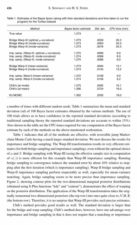
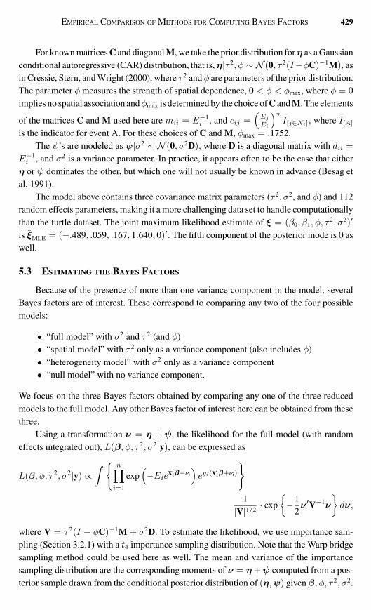groups or clusters are addressed by incorporating a set of random effects parameters in themodel In many applications the magnitude of the variance components corresponding toone or more of the sets of random effects are of interest especially the point null hypothesisthat the variance components in question are equal to zero A Bayesian approach for testinga hypothesis of this type is to compute the Bayes factor comparing the models suggested bythe null and the alternative hypotheses The primary objective of this work is to apply andevaluate the performance of different approaches for estimating the Bayes factor comparingthe GLMMs

A number of related studies exist in the statistical literature Albert and Chib (1997)provided a broad survey of the use of Bayes factors for judging a variety of assumptionsincluding assumptions regarding the variance components in conditionally independenthierarchical models (which include GLMMs as a special case) Han and Carlin (2001) pro-vided a review and empirical comparison of several Markov chain Monte Carlo (MCMC)methods for estimating Bayes factors emphasizing normal linear mixed model applica-tions Their study does not include importance sampling or warp bridge sampling PaulerWakefield and Kass (1999) provided a number of analytic approximations for comput-ing Bayes factors for variance component testing in linear mixed models DiCiccio KassRaftery and Wasserman (1997) compared several simulation-based approximation meth-ods for estimating Bayes factors Their study was quite general whereas the present workfocuses on GLMMs The present study adds to the literature by focussing on GLMMs (morespecifically on testing variance components in GLMMs) incorporating complex GLMMswith multiple variance components and incorporating new developments like warp bridgesampling (Meng and Schilling 2003) Our work should be of great interest to researchersworking with GLMMs but others will also find the results especially the findings on warpbridge sampling useful

Section 2 discusses a number of preliminary ideas regarding GLMMs Section 3 re-views the Bayes factor and approaches for estimating it Section 4 compares the differentapproaches in the context of a random effects probit regression model applied to data froma natural selection study (Janzen Tucker and Paukstis 2000) Section 5 takes up a morecomplex example a Poisson-normal regression model with spatial random effects and het-erogeneity random effects applied to Scotland lip-cancer data (Clayton and Kaldor 1987)Section 6 provides a discussion of our findings and recommendations

2 PRELIMINARIES

21 THE GENERALIZED LINEAR MIXED MODEL

In a GLMM observations y1 y2 yn are modeled as independent given canonicalparameters ξirsquos and a scale parameter φ with density

f(yi|ξi φ) = exp[yiξi minus a(ξi) + b(yi)]φ








L(αθ|y) =int

b

nprod

i=1

f(yi|ξi)

f(b|θ)db =

intb

nprod

i=1

f(yi|αb)





3 BAYES FACTORS

31 INTRODUCTION









p(M0)p(M1)

(31)








p(y|M) =int


d(ω)dω


p(y|M) asymp 1N

Nsumi=1

q(ωi|yM)d(ωi)







p(ω|yM)middot (32)




323 Bridge Sampling



(33)



r asymp1n2

sumn2


sumn1



r(t+1) =1n2

n2sumj=1

l2j

s1l2j + s2r(t)

1n1

n1sumj=1

1s1l1j + s2r(t)

(34)

where sk = nk



sumn2

j=1q(ωωωj |yM)










l1j =|S|2


and

l2j =|S|2



sumj

radic1


)











min



∣∣∣∣





Njprime

πj

πjprime middot

325 Other Methods


33 PARAMETERIZATION



p(y) =int int


=int int int















p(y|M0) =int


and

p(y|M1) =int
















43 RESULTS












RJ MCMC 1302 2032 180













1 9 28 16 138 4 5 9 11 192 39 231 16 866 2 7 103 11 83 10 304 2 6 124 9 52 24 253 3 18 20 28

54 1 247 1 703 5 34 38 49 51 5255 0 103 16 416 5 18 20 24 27 5656 0 39 10 176 6 18 24 30 33 45 55











(Ej

Ei





2 σ2)prime








nprodi=1

exp(minusEie

xprimeiβββ+νi

)eyi(xprime

iβββ+νi)

1|V|12

middot exp

minus1

2νprimeVminus1ν

dν


















RJMCMC 121 265 499




RJMCMC 032 182 309





55 RESULTS






















REFERENCES




































L(αθ|y) =int

b

nprod

i=1

f(yi|ξi)

f(b|θ)db =

intb

nprod

i=1

f(yi|αb)





3 BAYES FACTORS

31 INTRODUCTION









p(M0)p(M1)

(31)








p(y|M) =int


d(ω)dω


p(y|M) asymp 1N

Nsumi=1

q(ωi|yM)d(ωi)







p(ω|yM)middot (32)




323 Bridge Sampling



(33)



r asymp1n2

sumn2


sumn1



r(t+1) =1n2

n2sumj=1

l2j

s1l2j + s2r(t)

1n1

n1sumj=1

1s1l1j + s2r(t)

(34)

where sk = nk



sumn2

j=1q(ωωωj |yM)










l1j =|S|2


and

l2j =|S|2



sumj

radic1


)











min



∣∣∣∣





Njprime

πj

πjprime middot

325 Other Methods


33 PARAMETERIZATION



p(y) =int int


=int int int















p(y|M0) =int


and

p(y|M1) =int
















43 RESULTS












RJ MCMC 1302 2032 180













1 9 28 16 138 4 5 9 11 192 39 231 16 866 2 7 103 11 83 10 304 2 6 124 9 52 24 253 3 18 20 28

54 1 247 1 703 5 34 38 49 51 5255 0 103 16 416 5 18 20 24 27 5656 0 39 10 176 6 18 24 30 33 45 55











(Ej

Ei





2 σ2)prime








nprodi=1

exp(minusEie

xprimeiβββ+νi

)eyi(xprime

iβββ+νi)

1|V|12

middot exp

minus1

2νprimeVminus1ν

dν


















RJMCMC 121 265 499




RJMCMC 032 182 309





55 RESULTS






















REFERENCES
































p(M0)p(M1)

(31)








p(y|M) =int


d(ω)dω


p(y|M) asymp 1N

Nsumi=1

q(ωi|yM)d(ωi)







p(ω|yM)middot (32)




323 Bridge Sampling



(33)



r asymp1n2

sumn2


sumn1



r(t+1) =1n2

n2sumj=1

l2j

s1l2j + s2r(t)

1n1

n1sumj=1

1s1l1j + s2r(t)

(34)

where sk = nk



sumn2

j=1q(ωωωj |yM)










l1j =|S|2


and

l2j =|S|2



sumj

radic1


)











min



∣∣∣∣





Njprime

πj

πjprime middot

325 Other Methods


33 PARAMETERIZATION



p(y) =int int


=int int int















p(y|M0) =int


and

p(y|M1) =int
















43 RESULTS












RJ MCMC 1302 2032 180













1 9 28 16 138 4 5 9 11 192 39 231 16 866 2 7 103 11 83 10 304 2 6 124 9 52 24 253 3 18 20 28

54 1 247 1 703 5 34 38 49 51 5255 0 103 16 416 5 18 20 24 27 5656 0 39 10 176 6 18 24 30 33 45 55











(Ej

Ei





2 σ2)prime








nprodi=1

exp(minusEie

xprimeiβββ+νi

)eyi(xprime

iβββ+νi)

1|V|12

middot exp

minus1

2νprimeVminus1ν

dν


















RJMCMC 121 265 499




RJMCMC 032 182 309





55 RESULTS






















REFERENCES


































p(ω|yM)middot (32)




323 Bridge Sampling



(33)



r asymp1n2

sumn2


sumn1



r(t+1) =1n2

n2sumj=1

l2j

s1l2j + s2r(t)

1n1

n1sumj=1

1s1l1j + s2r(t)

(34)

where sk = nk



sumn2

j=1q(ωωωj |yM)










l1j =|S|2


and

l2j =|S|2



sumj

radic1


)











min



∣∣∣∣





Njprime

πj

πjprime middot

325 Other Methods


33 PARAMETERIZATION



p(y) =int int


=int int int















p(y|M0) =int


and

p(y|M1) =int
















43 RESULTS












RJ MCMC 1302 2032 180













1 9 28 16 138 4 5 9 11 192 39 231 16 866 2 7 103 11 83 10 304 2 6 124 9 52 24 253 3 18 20 28

54 1 247 1 703 5 34 38 49 51 5255 0 103 16 416 5 18 20 24 27 5656 0 39 10 176 6 18 24 30 33 45 55











(Ej

Ei





2 σ2)prime








nprodi=1

exp(minusEie

xprimeiβββ+νi

)eyi(xprime

iβββ+νi)

1|V|12

middot exp

minus1

2νprimeVminus1ν

dν


















RJMCMC 121 265 499




RJMCMC 032 182 309





55 RESULTS






















REFERENCES































r asymp1n2

sumn2


sumn1



r(t+1) =1n2

n2sumj=1

l2j

s1l2j + s2r(t)

1n1

n1sumj=1

1s1l1j + s2r(t)

(34)

where sk = nk



sumn2

j=1q(ωωωj |yM)










l1j =|S|2


and

l2j =|S|2



sumj

radic1


)











min



∣∣∣∣





Njprime

πj

πjprime middot

325 Other Methods


33 PARAMETERIZATION



p(y) =int int


=int int int















p(y|M0) =int


and

p(y|M1) =int
















43 RESULTS












RJ MCMC 1302 2032 180













1 9 28 16 138 4 5 9 11 192 39 231 16 866 2 7 103 11 83 10 304 2 6 124 9 52 24 253 3 18 20 28

54 1 247 1 703 5 34 38 49 51 5255 0 103 16 416 5 18 20 24 27 5656 0 39 10 176 6 18 24 30 33 45 55











(Ej

Ei





2 σ2)prime








nprodi=1

exp(minusEie

xprimeiβββ+νi

)eyi(xprime

iβββ+νi)

1|V|12

middot exp

minus1

2νprimeVminus1ν

dν


















RJMCMC 121 265 499




RJMCMC 032 182 309





55 RESULTS






















REFERENCES































l1j =|S|2


and

l2j =|S|2



sumj

radic1


)











min



∣∣∣∣





Njprime

πj

πjprime middot

325 Other Methods


33 PARAMETERIZATION



p(y) =int int


=int int int















p(y|M0) =int


and

p(y|M1) =int
















43 RESULTS












RJ MCMC 1302 2032 180













1 9 28 16 138 4 5 9 11 192 39 231 16 866 2 7 103 11 83 10 304 2 6 124 9 52 24 253 3 18 20 28

54 1 247 1 703 5 34 38 49 51 5255 0 103 16 416 5 18 20 24 27 5656 0 39 10 176 6 18 24 30 33 45 55











(Ej

Ei





2 σ2)prime








nprodi=1

exp(minusEie

xprimeiβββ+νi

)eyi(xprime

iβββ+νi)

1|V|12

middot exp

minus1

2νprimeVminus1ν

dν


















RJMCMC 121 265 499




RJMCMC 032 182 309





55 RESULTS






















REFERENCES

































Njprime

πj

πjprime middot

325 Other Methods


33 PARAMETERIZATION



p(y) =int int


=int int int















p(y|M0) =int


and

p(y|M1) =int
















43 RESULTS












RJ MCMC 1302 2032 180













1 9 28 16 138 4 5 9 11 192 39 231 16 866 2 7 103 11 83 10 304 2 6 124 9 52 24 253 3 18 20 28

54 1 247 1 703 5 34 38 49 51 5255 0 103 16 416 5 18 20 24 27 5656 0 39 10 176 6 18 24 30 33 45 55











(Ej

Ei





2 σ2)prime








nprodi=1

exp(minusEie

xprimeiβββ+νi

)eyi(xprime

iβββ+νi)

1|V|12

middot exp

minus1

2νprimeVminus1ν

dν


















RJMCMC 121 265 499




RJMCMC 032 182 309





55 RESULTS






















REFERENCES










































p(y|M0) =int


and

p(y|M1) =int
















43 RESULTS












RJ MCMC 1302 2032 180













1 9 28 16 138 4 5 9 11 192 39 231 16 866 2 7 103 11 83 10 304 2 6 124 9 52 24 253 3 18 20 28

54 1 247 1 703 5 34 38 49 51 5255 0 103 16 416 5 18 20 24 27 5656 0 39 10 176 6 18 24 30 33 45 55











(Ej

Ei





2 σ2)prime








nprodi=1

exp(minusEie

xprimeiβββ+νi

)eyi(xprime

iβββ+νi)

1|V|12

middot exp

minus1

2νprimeVminus1ν

dν


















RJMCMC 121 265 499




RJMCMC 032 182 309





55 RESULTS






















REFERENCES



































43 RESULTS












RJ MCMC 1302 2032 180













1 9 28 16 138 4 5 9 11 192 39 231 16 866 2 7 103 11 83 10 304 2 6 124 9 52 24 253 3 18 20 28

54 1 247 1 703 5 34 38 49 51 5255 0 103 16 416 5 18 20 24 27 5656 0 39 10 176 6 18 24 30 33 45 55











(Ej

Ei





2 σ2)prime








nprodi=1

exp(minusEie

xprimeiβββ+νi

)eyi(xprime

iβββ+νi)

1|V|12

middot exp

minus1

2νprimeVminus1ν

dν


















RJMCMC 121 265 499




RJMCMC 032 182 309





55 RESULTS






















REFERENCES






































RJ MCMC 1302 2032 180













1 9 28 16 138 4 5 9 11 192 39 231 16 866 2 7 103 11 83 10 304 2 6 124 9 52 24 253 3 18 20 28

54 1 247 1 703 5 34 38 49 51 5255 0 103 16 416 5 18 20 24 27 5656 0 39 10 176 6 18 24 30 33 45 55











(Ej

Ei





2 σ2)prime








nprodi=1

exp(minusEie

xprimeiβββ+νi

)eyi(xprime

iβββ+νi)

1|V|12

middot exp

minus1

2νprimeVminus1ν

dν


















RJMCMC 121 265 499




RJMCMC 032 182 309





55 RESULTS






















REFERENCES






































1 9 28 16 138 4 5 9 11 192 39 231 16 866 2 7 103 11 83 10 304 2 6 124 9 52 24 253 3 18 20 28

54 1 247 1 703 5 34 38 49 51 5255 0 103 16 416 5 18 20 24 27 5656 0 39 10 176 6 18 24 30 33 45 55











(Ej

Ei





2 σ2)prime








nprodi=1

exp(minusEie

xprimeiβββ+νi

)eyi(xprime

iβββ+νi)

1|V|12

middot exp

minus1

2νprimeVminus1ν

dν


















RJMCMC 121 265 499




RJMCMC 032 182 309





55 RESULTS






















REFERENCES
































(Ej

Ei





2 σ2)prime








nprodi=1

exp(minusEie

xprimeiβββ+νi

)eyi(xprime

iβββ+νi)

1|V|12

middot exp

minus1

2νprimeVminus1ν

dν


















RJMCMC 121 265 499




RJMCMC 032 182 309





55 RESULTS






















REFERENCES













































RJMCMC 121 265 499




RJMCMC 032 182 309





55 RESULTS






















REFERENCES
















































REFERENCES





























an empirical comparison of methods for computing bayes factors

Documents