an empirical evaluation of monetary and fiscal policy effects in … · fiscal policy effects in...

ASIAN DEVELOPMENT BANK

AsiAn Development BAnk6 ADB Avenue, Mandaluyong City1550 Metro Manila, Philippineswww.adb.org

An EmpiricAl EvAluAtion of monEtAry And fiscAl policy EffEcts in BAnglAdEshMd. Shahnawaz Karim

ADB South ASiA Working PAPer SerieS

no. 66

August 2019

An Empirical Evaluation of monetary and fiscal policy Effects in Bangladesh

Macroeconomic policy management is crucial for attaining sustainable economic growth with a stable rate of inflation. This working paper examines monetary and fiscal policies in Bangladesh and their effectiveness in achieving sustainable growth and price stability. It concludes that Bangladesh should focus on a combination of expansionary monetary policies and restrictive fiscal policies as the most beneficial approach.

About the Asian development Bank

ADB is committed to achieving a prosperous, inclusive, resilient, and sustainable Asia and the Pacific, while sustaining its efforts to eradicate extreme poverty. Established in 1966, it is owned by 68 members —49 from the region. Its main instruments for helping its developing member countries are policy dialogue, loans, equity investments, guarantees, grants, and technical assistance.

Md. Shahnawaz Karim

No. 66 | August 2019

Md. Shahnawaz Karim, PhD, is an associate professor at the Economics Department, School of Business, of the Independent University in Bangladesh.

ADB South Asia Working Paper Series

An Empirical Evaluation of Monetary and Fiscal Policy Effects in Bangladesh


Creative Commons Attribution 3.0 IGO license (CC BY 3.0 IGO)

© 2019 Asian Development Bank6 ADB Avenue, Mandaluyong City, 1550 Metro Manila, PhilippinesTel +63 2 632 4444; Fax +63 2 636 2444www.adb.org

Some rights reserved. Published in 2019.Printed in the Philippines.

ISSN 2313-5867 (print), 2313-5875 (electronic)Publication Stock No. WPS190285-2DOI: http://dx.doi.org/10.22617/WPS190285-2

The views expressed in this publication are those of the authors and do not necessarily reflect the views and policies of the Asian Development Bank (ADB) or its Board of Governors or the governments they represent.

ADB does not guarantee the accuracy of the data included in this publication and accepts no responsibility for any consequence of their use. The mention of specific companies or products of manufacturers does not imply that they are endorsed or recommended by ADB in preference to others of a similar nature that are not mentioned.

By making any designation of or reference to a particular territory or geographic area, or by using the term “country” in this document, ADB does not intend to make any judgments as to the legal or other status of any territory or area.

This work is available under the Creative Commons Attribution 3.0 IGO license (CC BY 3.0 IGO) https://creativecommons.org/licenses/by/3.0/igo/. By using the content of this publication, you agree to be bound by the terms of this license. For attribution, translations, adaptations, and permissions, please read the provisions and terms of use at https://www.adb.org/terms-use#openaccess.

This CC license does not apply to non-ADB copyright materials in this publication. If the material is attributed to another source, please contact the copyright owner or publisher of that source for permission to reproduce it. ADB cannot be held liable for any claims that arise as a result of your use of the material.

Please contact [email protected] if you have questions or comments with respect to content, or if you wish to obtain copyright permission for your intended use that does not fall within these terms, or for permission to use the ADB logo.

The ADB South Asia Working Paper Series is a forum for ongoing and recently completed research and policy studies undertaken in ADB or on its behalf. It is meant to enhance greater understanding of current important economic and development issues in South Asia, promote policy dialogue among stakeholders, and facilitate reforms and development management.

The ADB South Asia Working Paper Series is a quick-disseminating, informal publication whose titles could subsequently be revised for publication as articles in professional journals or chapters in books. The series is maintained by the South Asia Department. The series will be made available on the ADB website and on hard copy.

Corrigenda to ADB publications may be found at http://www.adb.org/publications/corrigenda.

Notes:In this publication, “$” refers to United States dollars and “Tk” refers to the taka.

www.adb.org

http://dx.doi.org/10.22617/WPS190285

https://creativecommons.org/licenses/by/3.0/igo

https://www.adb.org/terms

mailto:[email protected]

http://www.adb.org/publications/corrigenda

CONTENTS

TABLE AND FIGURES iv

EXECUTIVE SUMMARY v

I. INTRODUCTION 1

A. Inflation Scenario in Bangladesh 1

II. BRIEF DESCRIPTION OF SOME BASIC MACROECONOMIC INDICATORS OF BANGLADESH 3

III. BRIEF TREATISE ON THEORETICAL AND EMPIRICAL LITERATURE 5

IV. CONSTRUCTION OF THE STRUCTURAL VECTOR AUTOREGRESSIVE MODEL 7

V. IDENTIFICATION OF THE STRUCTURAL SHOCKS 10

VI. EMPIRICAL MODELS AND IDENTIFICATION ISSUES 11

A. Theory-Guided Restrictions Imposed on the Contemporaneous Matrix 11 B. Restrictions Imposed in Accordance with Choleskey Decomposition Method 12

VII. DATA AND MODEL ESTIMATION 12

VIII. IMPULSE RESPONSE FUNCTIONS 13

A. Impulse Responses of Non-Policy Variables due to Structural Monetary Policy Shocks 13

B. Impulse Responses of Non-Policy Variables due to Structural Fiscal Policy Shocks 16 C. Impulse Responses of Non-Policy Variables due to Policy Shocks Identified

by Choleskey Factorization Method 18

IX. CONCLUSION 25

APPENDIXES

1 Selection of Lag Length in the Level VAR Model 27 2 Lag Exclusion Wald Test in the Level VAR Model 28 3 Contemporaneous Pattern Matrices of the SVAR Model 29 4 Estimated Contemporaneous Coefficient Matrix and the LR Test

on Contemporaneous Restrictions 30

REFERENCES 31

TABLE AND FIGURES

TABLE 1 Consumer Price Index Inflation Rate Under Different Classifications 2

FIGURES 1 Annual Gross Domestic Product and Government Consumption of Bangladesh 3 2 Annual Percentage Growth Rate of Real Gross Domestic Product and Government

Final Consumption of Bangladesh 4 3 Bangladesh Annual Lending Interest Rate, Inflation Rate, and Appreciation/Depreciation

Rate of US Dollar against Taka 5 4 Impulse Responses of Variables Due to Monetary Expansion: SVAR Method 14 5 Impulse Responses of Variables Due to Monetary Contraction: SVAR Method 15 6 Impulse Responses of Variables to Fiscal Expansion: SVAR Method 17 7 Impulse Responses of Variables to Fiscal Restriction: SVAR Method 18 8 Impulse Responses of Variables to Monetary Expansion: Choleskey Method 20 9 Annual Net Inflow of Foreign Direct Investment as a Percentage

of Gross Domestic Product 21 10 Impulse Responses of Variables to Monetary Contraction: Choleskey Method 22 11 Impulse Responses of Variables to Fiscal Expansion: Choleskey Method 23 12 Impulse Responses of Variables to Fiscal Contraction: Choleskey Method 24

EXECUTIVE SUMMARY

Efficient macroeconomic policy management is essential for attaining sustainable economic growth with a stable inflation rate. Monetary and fiscal policies are two measures of macroeconomic management. The government may conduct a restrictive monetary policy either by reducing the money supply or by increasing the policy interest rate. On the contrary, the government may implement an expansionary monetary policy either by increasing the money supply or by reducing the policy interest rate.

This paper empirically examines the effectiveness of these measures with the aid of structural vector autoregressive (SVAR) and Choleskey factorization methods applying time series data on policy and non-policy macro variables of Bangladesh covering a period fiscal year (FY) 1971–2017.

Empirical analysis of this paper finds that a monetary expansion increases real gross domestic product (GDP) and overall price level on impact and causes an appreciation of the United States (US) dollar exchange rate against Taka. In addition, a fiscal expansionary shock increases overall domestic price level and causes a depreciation of the dollar vis-à-vis the taka. On the other hand, an expansionary fiscal policy shock imparts a delayed expansionary effect on real GDP because of the way the policy is implemented. The simulation study of this paper argues that a fiscal expansion in Bangladesh is financed by selling more government bonds with a higher interest that in turn mutes investment and eventual output growth initially, but consequently increases real GDP after a year that lasts for several years. On the other hand, a monetary contraction reduces output on impact, but exerts a delayed constricting effect on price level due to profit motivated pricing policies of producers in general. Simulation study also finds that a restrictive fiscal policy shock reduces real GDP and price level on impact but causes an appreciation of the taka against the dollar. In general, the empirical findings of this paper display asymmetric effects of monetary and fiscal policy measures. As quarterly and monthly data on macro variables of Bangladesh are not available, this paper utilizes annual data on these variables and assumes there is no implementation lag in case of the real effects of fiscal policy shocks and obtains plausible behavior of non-policy macro variables in general with some noticeable policy implications.

Overall, the simulation study finds that expansionary monetary and restrictive fiscal policies act more rapidly while attaining the desired outcomes than restrictive monetary and expansionary fiscal policy actions. Empirical observations of this paper suggest that capital market transactions in the country should be more integrated than before to make the direct channel of government monetary transmission more effective. On the other hand, the government can make its policy actions more effective by managing its tax revenue and capital expenditure more judiciously. It appears imperative for the government to implement remedial policy actions as the nation is looking forward to achieving a higher economic growth with a stable price in upcoming future.

I. INTRODUCTION

Bangladesh has been able to maintain an average real gross domestic product (GDP) growth of 6.5% from fiscal year (FY) 2009 to 2018.1 In FY2016–FY2018, the country succeeded in attaining more than 7% real GDP growth. It has also been capable of maintaining a stable inflation rate at 5.7% on average during FY2016–FY2018 in spite of rising growth. For Bangladesh to attain the status of an upper middle-income country, it has to maintain relatively low inflation amid increasing growth.

This paper used the GDP deflator as a measure of the domestic price level. It compiled data on the GDP deflator from the World Economic Outlook (WEO) database.2 Simulation studies similar to the one presented in this paper are highly sensitive to the number of observations on policy and non-policy variables used in model estimation. Considering this issue, this paper utilizes time series data on GDP deflator instead of consumer price index (CPI) data while estimating the empirical model for simulation analysis. While time series data on GDP deflator spans from FY1971 till FY2017, CPI data extends between FY1986–FY2017. However, the GDP deflator of Bangladesh is computed using FY2006 as the base year, while the CPI is calculated using FY2010 as the base year. Despite this minor dissimilarity, GDP deflator and CPI series are highly correlated. Correlation coefficient of the GDP deflator and the CPI series (FY1986–FY2017) is found to be 0.9986. The inflation rate of the GDP deflator has gone up from 5.87% in FY2015 to 6.73% in FY2016 and slightly declined to 6.28% in FY2017. On the other hand, the CPI inflation rate declined from FY6.19% in 2015 to 5.43% in FY2016 and increased to 5.78% in FY2017.

Two independent sets of commodities (goods and services) are used to compute CPIs for rural and urban areas. A rural basket covers 318 items while the urban basket consists of 422 commodities. The national CPI is calculated by combining the urban and rural indices using weight factors. The CPI items for the national and subnational indices have been classified into eight major groups, such as (i) food, beverage, and tobacco; (ii) clothing and footwear; (iii) gross rent, fuel, and lighting; (iv) furniture, furnishing, household equipment, and operation; (v) medical care and health expenses; (vi) transport and communications; (vii) recreation, entertainment, education, and cultural services; and (viii) miscellaneous goods and services.3

A. Inflation Scenario in Bangladesh

The CPI inflation scenario in Bangladesh should be observed focusing on sources (food or non-food) along with regional (urban or rural) share. Table 1 displays the breakdown of inflation rate for different CPI classifications.

1 The fiscal year (FY) of the Government of Bangladesh ends on 30 June. “FY” before a calendar year denotes the year in which the fiscal year ends, e.g., FY2018 ends on 30 June 2018.

2 International Monetary Fund. World Economic Outlook Database. https://www.imf.org/external/pubs/ft/weo/2018/02/weodata/index.aspx (accessed 1 December 2018).

3 Government of Bangladesh, Bureau of Statistics. 2018. Consumer Price Index (CPI), Inflation Rate and Wage Rate Index (WRI) in Bangladesh. February. http://bbs.portal.gov.bd/sites/default/files/files/bbs.portal.gov.bd/page/9ead9eb1_91ac_4998_a1a3_a5caf4ddc4c6/CPI_February18.pdf.

https://www.imf.org/external/pubs/ft/weo/2018/02/weodata/index.aspx

https://www.imf.org/external/pubs/ft/weo/2018/02/weodata/index.aspx

http://bbs.portal.gov.bd/sites/default/files/files/bbs.portal.gov.bd/page/9ead9eb1_91ac_4998_a1a3_a5caf4ddc4c6/CPI_February18.pdf


2 ADB South Asia Working Paper Series No. 66

Table 1: Consumer Price Index Inflation Rate Under Different Classifications

CPI Classification

Inflation RateDecember 2016

(%)December 2017

(%)February 2018

(%)Urban general index 6.07 5.82 5.87Urban food index 6.74 7.22 8.02Urban non-food index 5.35 4.25 3.50Rural general index 4.46 5.84 5.64Rural food index 4.78 7.08 6.94Rural non-food index 3.88 3.54 3.25National general index 5.03 5.83 5.72National food index 5.38 7.13 7.27National non-food index 4.49 3.85 3.36

CPI = consumer price index.Source: Government of Bangladesh, Bureau of Statistics. 2018. Consumer Price Index (CPI), Inflation Rate and Wage Rate Index (WRI) in Bangladesh. February. http://bbs.portal.gov.bd/sites/default/files/files/bbs.portal.gov.bd/page/9ead9eb1_91ac_4998_a1a3_a5caf4ddc4c6/CPI_February18.pdf.

Table 1 shows that national CPI inflation rate increased from December 2016 to December 2017, but declined slightly in February 2018. It can also be deduced that food price increase is responsible for this increase in overall CPI inflation rate, as the inflation rate of national food price index has gone up from December 2016 to February 2018. On the other hand, non-food price inflation rate from December 2016 to February 2018 stayed within the range of 4.49%–3.36%. It can also be observed that urban food price inflation is mainly responsible for this increase in the overall CPI inflation rate as the inflation rate of the urban food price index has gone up from 6.74% in December 2016 to 7.22% in December 2017 and finally to 8.02% in February 2018. In contrast, urban non-food price inflation rate declined from 5.35% in December 2016 to 4.25% in December 2017 and further to 3.50% in February 2018. The food price inflation rate in rural areas had also gone up from 4.78% in December 2016 to 7.08% in December 2017 with a slight decline to 6.94% in February 2018. Thus, urban food price inflation can be considered responsible for an increase in overall CPI inflation rate in Bangladesh in recent years.

If increasing growth is accorded with rising inflation, people will suffer from falling real income, their purchasing power will decline, and so will household consumption and aggregate demand. Eventually, private investment will decline and so will economic growth. Therefore, in the face of rising economic growth, Bangladesh needs to implement a judiciously concerted monetary and fiscal policy mix to maintain low and stable inflation rates. This paper empirically examines impact responses of domestic price level, output, and exchange rate due to monetary policy shocks that are both expansionary and restrictive in nature. This paper also evaluates expansionary and restrictive fiscal policy effects of domestic output and related variables. Unlike monetary policy, fiscal policy does not respond instantaneously due to sluggish real GDP growth. While a monetary policy may respond almost immediately due to rising inflation for instance, fiscal policy does the same to a sluggish real GDP growth, but with a time lag as it takes time for an approval of a fiscal policy change by legislation before being actually implemented. As a result, an expansionary fiscal policy action may impart a delayed effect on real GDP.



An Empirical Evaluation of Monetary and Fiscal Policy Effects in Bangladesh 3

This paper empirically examines the effects of monetary and fiscal policy stances on real GDP, price level, and exchange rate of Bangladesh with the aid of the SVAR method. Empirical findings of the paper may have important implications for prudent macroeconomic policy management. For empirical analysis, annual data on policy and non-policy macro variables of Bangladesh have been used in this paper. Empirical literature indicates that effects of restrictive monetary policy shocks on real GDP, domestic inflation, and exchange rate can be observed almost instantly, while the effects of expansionary fiscal policy shocks on real GDP may be observed with a time lag due to implementation delays of such policy changes. Since annual data on all policy and non-policy macro variables are used, it is assumed that monetary and fiscal policy effects of non- policy variables can be observed at most within a year.

II. BRIEF DESCRIPTION OF SOME BASIC MACROECONOMIC INDICATORS OF BANGLADESH

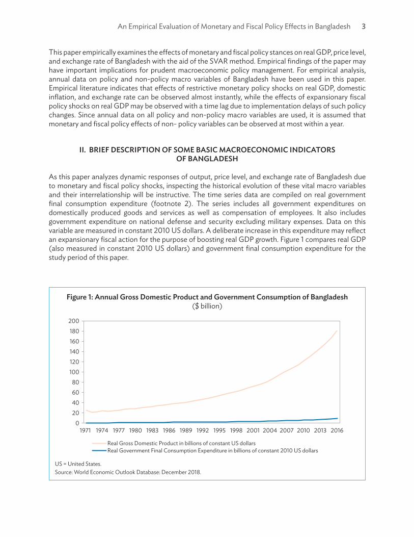
As this paper analyzes dynamic responses of output, price level, and exchange rate of Bangladesh due to monetary and fiscal policy shocks, inspecting the historical evolution of these vital macro variables and their interrelationship will be instructive. The time series data are compiled on real government final consumption expenditure (footnote 2). The series includes all government expenditures on domestically produced goods and services as well as compensation of employees. It also includes government expenditure on national defense and security excluding military expenses. Data on this variable are measured in constant 2010 US dollars. A deliberate increase in this expenditure may reflect an expansionary fiscal action for the purpose of boosting real GDP growth. Figure 1 compares real GDP (also measured in constant 2010 US dollars) and government final consumption expenditure for the study period of this paper.

US = United States.Source: World Economic Outlook Database: December 2018.

Figure 1: Annual Gross Domestic Product and Government Consumption of Bangladesh ($ billion)

020406080

100120140160180

200

1971

Real Gross Domestic Product in billions of constant US dollarsReal Government Final Consumption Expenditure in billions of constant 2010 US dollars

1974 1977 1980 1983 1986 1989 1992 1995 1998 2001 2004 2007 2010 2013 2016


Figure 1 shows an increasing trend in real GDP of Bangladesh along with a gradual increase in government final consumption expenditure since FY1971. The figure indicates that deliberate expansion of government final consumption expenditure might have a positive association with real GDP over time. The probable reason of this positive association might be that increased government final consumption might have enhanced disposable real income of households inducing expenditure on domestically produced goods and services and eventually expanding real GDP over the period FY1971–FY2017.

Figure 2 displays annual growth rates of real GDP and real government final consumption expenditure of Bangladesh from FY1977 to FY2016. These variables displayed some aberrant growth rates from FY1972 to FY1976 and the 4-year period was thus not considered for discussion. Starting FY1981, the growth rate of real GDP shows a consistent co-movement with that of real government final consumption expenditure. More specifically, a fall in real government final consumption expenditure is followed by a decline in real GDP growth rate and vice versa. This type of co-movement between growth rates of real government final consumption and real GDP is also visible during FY1998–FY2000. In more recent times, when the growth rate of real government final consumption expenses increased from 5.8% in FY2013 to 8.8% in FY2015, the growth rate of real GDP increased from 6% to 6.6% over the same period. These observations are indicative of a primary evidence of a positive association of expansionary fiscal policy and real GDP growth rate.

Figure 3 displays historical movements of lending interest rate, appreciation or depreciation of the dollar against the taka, and inflation rate of GDP deflator. It is conspicuous that movements of lending rate are rather stable compared to fluctuations in exchange rate (appreciation or depreciation) and inflation rate. It can also be noted that an upward movement of landing rate is associated with a downfall in the inflation rate. For instance, when lending rate increases from 12% in FY1985 to 14% in FY1986, inflation rate falls from 18.5% to 8.25%, whereas the appreciation rate of the dollar against the taka falls from 10.4% to 8.6% over the same period. When interest rates went up from 12.76% in 2000 to 12.82% in 2001, the

Figure 2: Annual Percentage Growth Rate of Real Gross Domestic Product and Government Final Consumption of Bangladesh

GDP = gross domestic product.Source: World Economic Outlook Database: December 2018.

–50

0

50

100

%

150

200

1972

Growth rate of real GDPGrowth rate of real government final consumption expenditure

1976 1980 1984 1988 1992 1996 2000 2004 2008 2012 2016


inflation rate fell from 3.45% to 3.26% over the same period, although the US dollar appreciated from 6.2% to 7% over the same period.

From these rather sporadic movements of these variables, an upward movement of lending rate exerts a downward pressure on domestic inflation and reduces the appreciation rate of the dollar against the Taka. Despite the inconclusive nature of this observation, an increase in bank lending rate may be responsible for a decline in inflation rate and the appreciation rate of the dollar against the taka. An increase in bank lending rate possibly reflects a restrictive monetary policy stance of the government.

III. BRIEF TREATISE ON THEORETICAL AND EMPIRICAL LITERATURE

During the 1970s, economists used large simultaneous structural econometric models for forecasting and policy evaluation. Sims criticized these models for their inherent drawbacks, as these are incapable of producing accurate forecasts of macro variables in one hand and incompetent of estimating real effects of monetary and fiscal policy measures, on the other.4 Sims further pointed out that the inherent follies of large structural models during the 1970s lie in the way they categorize the relevant variables into two dichotomous groups, such as exogenous and endogenous. These models were also well-known for imposing impossible restrictions on the contemporaneous relationships among variables to identify policy shocks. According to Sims, it is virtually impossible to classify variables into two groups due to their inherent feedback relationships. Consequently, all variables are placed on equal footing and included as endogenous variables into Sims’ prototype vector auto regression (VAR) models, where every variable depends on its own past values and those of other variables. Since then, VAR models are used for short-term forecasting and policy evaluation. However, even VAR models are later criticized for

4 Sims (1980).

US = United States.Source: World Economic Outlook Database: December 2018.

Figure 3: Bangladesh Annual Lending Interest Rate, Inflation Rate, and Appreciation/Depreciation Rate of US Dollar against Taka

–40

–20

0

20

40

60

80

100

1971

Appreciation/Depreciation rate of US dollar against takaGDP deflator inflation rateLending interest rate

%

1975 1979 1983 1987 1991 1995 1999 2003 2007 2011 2015


being over parameterized and a-theoretic, although Sims pointed out that these models emphasize the dynamic relationships between variables more than their parameter estimates. On the other hand, VAR models are considered empirical counterparts of dynamic stochastic general equilibrium models and produce relatively reliable short-term forecasts.

Ample empirical literature has been published during the late 1990s and onward focusing on the dynamic effects of unexpected monetary policy shocks on money and real variables. More specifically, these papers have analyzed the dynamic responses of consumer price level, producer price level, and exchange rate (money variables) in one hand and real variables, such as output and employment on the other, due to unexpected positive shocks to policy interest rate (bank rate) or money supply. Some of this literature have successfully identified monetary policy shocks and consequently estimated the dynamic responses of money and real variables in line with the theoretical predictions. However, some of these research papers also reported empirical puzzles, such as price and exchange rate, in response to unexpected positive monetary policy shocks. Until the advent of the most recent episode of the global financial crisis in 2008, nations generally relied on monetary policy for stabilizing their economies when faced with adverse business cycle fluctuations.

When the global financial crisis ended, researchers began paying attention to discretionary fiscal policy measures for achieving targeted macroeconomic goals. Blanchard and Perotti (2002) used the SVAR approach for analyzing the fiscal policy effects of real variables, such as output and investment due to positive shocks to government expenses and tax revenue during postwar era in the United States (US). Using quarterly US data on government purchases, per capita real GDP, and net tax revenue for 1947–1997, Blanchard and Perotti analyzed the fiscal policy transmission mechanism. In particular, they estimated impulse response functions of per capita real GDP in response to positive shocks to government purchases and net tax revenue. However, Blanchard and Perotti had to identify the fiscal policy shock first and assumed there is a time lag between the legislation of a fiscal policy act and consequent response of real activity. Alternatively, they assumed there was no contemporaneous relationship between real GDP and government expenditure or net tax revenue (representing a restrictive fiscal policy shock) within a quarter. Given the quarterly data on these macro and fiscal policy variables, these zero restrictions (coefficients signifying relationships between model variables in the current period are set equal to zero) on contemporaneous variables helped them identifying unexpected fiscal policy shocks.

Ilzetzki, Mendoza, and Vegh (2013) used quarterly panel data covering 10 years for 44 countries with different economic status while analyzing the fiscal transmission mechanism under fixed and flexible exchange rate regimes. They also classified the countries under study in accordance with relatively open and closed economic status. However, their study differs from that of Blanchard and Perotti (2002) as Ilzetzki Mendoza, and Vegh (2013) failed to incorporate data on tax revenue and eventually seemed incapable of capturing the restrictive fiscal policy actions. Despite this limitation, their study shared a common feature with that of Blanchard et al. as both studies used a recursive Choleskey decomposition method while identifying the structural fiscal policy shocks from the residual error terms of the reduced form VAR models.

Leeper, Walker, and Yang (2008) criticized other studies that analyzed the fiscal transmission mechanism pointing to the omission of fiscal foresights of private economic agents that might influence their consumption, saving, and investment behavior at present. Unlike monetary policy, fiscal policy must be announced first and then approved by the legislative bodies before it can take effect. Consequently, anticipated fiscal policy change and ensuing responses of private economic agents may differ from that which is predicted by a researcher who has identified fiscal policy shock using an SVAR model.


Favero and Giavazzi (2012) pointed out that failure to incorporate fiscal foresight into the SVAR model of fiscal policy transmission makes the model noninvertible in its moving average presentation.

More recently, researchers have been emphasizing the interaction of fiscal and monetary policies and suggesting including this combined effect into the empirical SVAR model for the purpose of identifying the exogenous fiscal policy shocks and eventually estimating the impulse responses of relevant non-policy variables. Both Blanchard and Perotti (2002) and Christiano, Eichenbaum, and Vigfusson (2007) analyzed fiscal and monetary policy transmissions in separation from each other. The main difference between these studies lies in the way the fiscal and monetary policy shocks are identified. While Blanchard et al. recovered structural fiscal policy shocks from residual errors of the reduced form VAR model using a recursive Choleskey decomposition method, Christiano, Eichenbaum, and Vigfusson identified monetary policy shocks from the estimated model by imposing short run restrictions on the contemporaneous relationships among the policy and non-policy model variables. Sargent and Wallace (1981) built a theoretical macro model with the implication that monetary and fiscal policies interact with each other and should not be studied in isolation.

Apart from all these discussions relating to whether monetary and fiscal policies should be separately studied or a combination of these two policies needs to be analyzed, Leeper (1989) showed how a researcher may trace some incidents as monetary policy effects that are actually caused by a fiscal policy shock. Ramey (2011) showed that fiscal SVARs identify fiscal shocks that are not exogenous, but are quite anticipated.

Considering all the issues in relation to SVAR models of fiscal and monetary transmission, this study opts for adopting a combined monetary and fiscal policy SVAR model that incorporates fiscal foresights of private individual economic agents and consequently proposes to estimate and analyze the dynamic effects of these policies on real economic variables. As far as the fiscal policy is concerned, the empirical model assumes that an unanticipated tax shock is revealed in terms of an announced tax hike at the current period, while an anticipated tax shock is simulated by a tax hike announced in the previous period but not yet implemented.

IV. CONSTRUCTION OF THE STRUCTURAL VECTOR AUTOREGRESSIVE MODEL

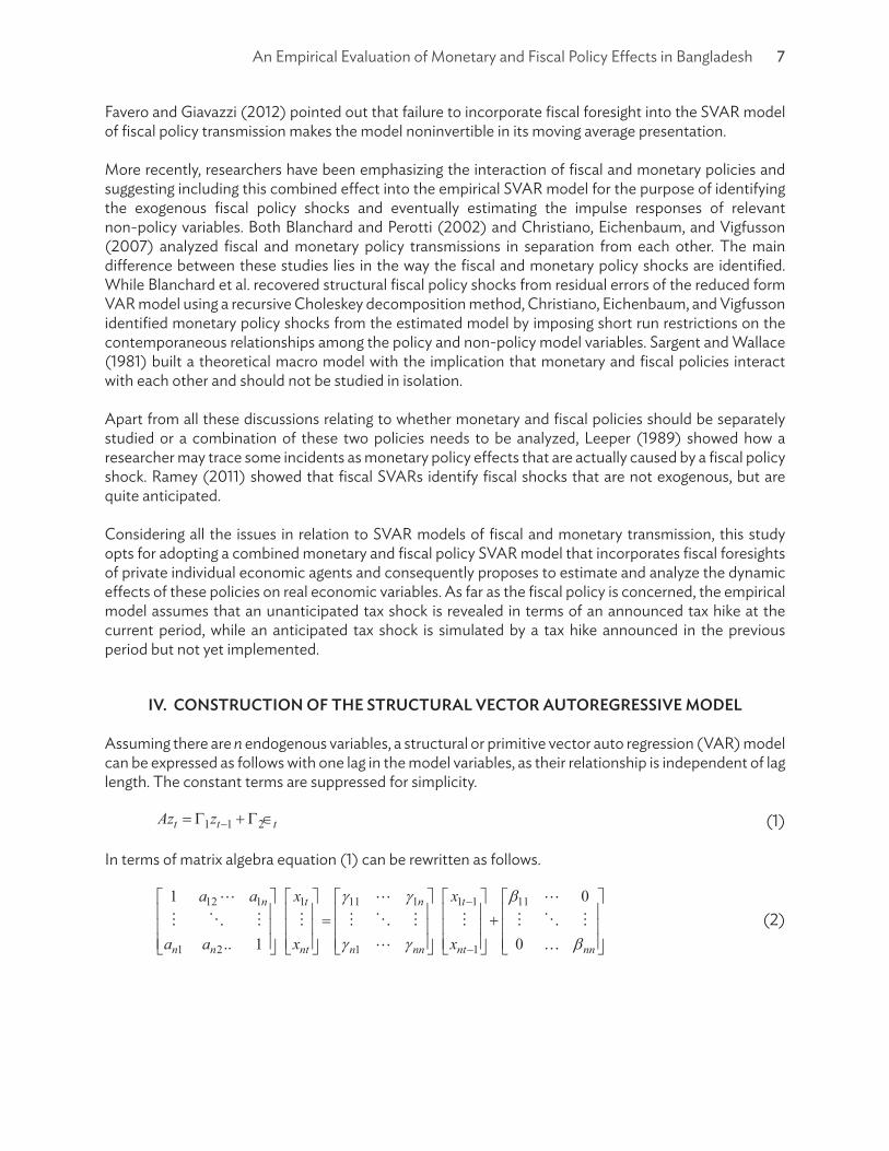
Assuming there are n endogenous variables, a structural or primitive vector auto regression (VAR) model can be expressed as follows with one lag in the model variables, as their relationship is independent of lag length. The constant terms are suppressed for simplicity.

1 1 2t t tAz z −= Γ + Γ ∈ (1)

In terms of matrix algebra equation (1) can be rewritten as follows.

12 1 1 11 1 1 1 11

1 2 1 1

1 0

.. 1 0

n t n t

n n nt n nn nt nn

a a x x

a a x x

γ γ β

γ γ β

−

−

= +

(2)


It is assumed that structural shocks are normally distributed with zero mean and constant variance. In other words, the variance–covariance matrix assumes the form ~ ( )t t nt

E Iε ε ε ′ = Γ∑ , where In is an

n dimensional identity matrix and

21

2

0

0 n

tε

σ

σ

=

∑

is an (nxn) square matrix, whose off diagonals

indicate zero covariance of the structural errors, and the principal diagonal indicates their constant variance.

Also, 12 1

1 2

1

.. 1

n

n n

a aA

a a

=

is an (nxn) matrix containing the contemporaneous coefficients

relating the endogenous variables and 11

2

0

0 nn

β

β

Γ =

is a diagonal matrix including

structural parameters.

1t

t

nt

xz

x

=

is an (nx1) vector of endogenous model variables.

11 1

1

1

n

n nn

γ γ

γ γ

Γ =

is an (nxn) matrix containing the coefficients of lagged endogenous variables.

1 1

1

1

t

t

nt

xz

x

−

−

−

=

is an (nx1) vector of lagged endogenous variables.

Finally, 1t

t

nt

ε

ε

∈ =

is an (nx1) vector of stochastic error terms that represent structural shocks and

1t

t

nt

ee

e

=

is an (nx1) vector of residual errors of the reduced form model.

VAR models are estimated using the ordinary least squares (OLS) method applied to each individual equation in the system, which produce efficient parameter estimates. However, equation (2) cannot be estimated using the OLS method as the error terms are correlated with right-hand side contemporaneous variables. Pre-multiplying both sides of equation (1), by A–1, and after rearranging the resulting matrices, a reduced form VAR model is derived as of equation (3), where the error terms are no longer correlated


with the right-hand side contemporaneous variables. Consequently, the OLS method can be applied to individual equations to obtain efficient parameter estimates.

1 1 11 1 2

1

t t t

t t t

A Az A z Ay By e

− − −−

−

= Γ + Γ ∈

= + (3)

Utilizing the fact that 1 1A A− = and letting 11A B− Γ = , and 1

2 t tA e− Γ ∈ = , equation (1) is rewritten as of equation (3). Using matrices and vectors, equation (3) is more explicitly expressed as equation (4). Equation (3) is a reduced form of model (1), where stand for the contemporaneous variable and for the lagged endogenous variable.

1 11 12 1 11 1 1 1 12 1 11 1

1 2 1 1 1 2

1 1 0

1 1 0

t n n t n t

nt n n n nn nt n n nn nt

y a a y a a

y a a y a a

γ γ β ε

γ γ β ε

− −−

−

= +

(4)

As the VAR models are over-parameterized, some of the model parameters may not be found to be statistically significant. Except for short-term forecasting, VAR models are estimated for monetary and fiscal policy analysis. From this standpoint, obtaining parameter estimates is not the main purpose of VAR modeling. Instead, the main objective of estimating the VAR models is identifying the structural shocks from the estimated error terms of the reduced form models. Structural shocks of the theoretical models are related to the estimated error terms of the reduced form models, as reflected by the equation

12 t tA e− Γ ∈ = . This relationship can be expressed as follows in case of the simplest possible VAR model

that includes only two endogenous variables. More explicitly, 12 t tA e− Γ ∈ = is shown in terms of matrices

and vectors as follows.

11 1 112 11 21 11

2 2 221 22 12 2212 21

1 0 1 011 0 1 01

t t t

t t t

e a ae a aa a

ε εβ βε εβ β

− − = = −−

(5)

According to equation (5), it may be concluded that the reduced form error terms are made up of structural shocks. Consequently, a shock to the reduced form error cannot be taken as a structural shock to the relevant endogenous variable.

Reverting to the relationship tying reduced form errors and structural shocks, there is 12 t tA e− Γ ∈ = .

Pre-multiplying the left and right hand sides of this equation and rearranging terms, it can be finally expressed as 2t tAe = Γ ∈ , which is known as the AB model proposed by Amisano and Giannini (1997). In case of an n variable structural model, the AB model can also be expressed as follows using matrices and vectors.

12 1 1 11 1

1 2

1 0

.. 1 0

n t t

n n nt nn nt

a a e

a a e

β ε

β ε

=

(6)

Equation (6) indicates that structural shocks are related to residual error terms of a VAR model in a definitive way. In other words, once a reduced form VAR model is estimated, structural shocks from reduced form residual error terms can be recovered or identified given that the contemporaneous matrix A is invertible. Pre multiplying both sides of (6) by A–1, the following equation can be derived, which aids in performing this task.


11 12 1 11 1

1 2

1 0

.. 1 0

t n t

nt n n nn nt

e a a

e a a

β ε

β ε

− =

(7)

Equation (7), which can be concisely written as 12t te A− Γ ∈= or alternatively, 1

t te A u−= , where 2t tu = Γ ∈ , is a composite term that contains the structural shocks. Transposing both sides of 1

t te A u−= and pre-multiplying both sides by themselves yield ( ) 11ee A uu A −−′ ′ ′= …(8). Taking expectations of both sides of equation (8) yields ( ) 11

e A A −− ′Σ = Ω …(9), where Σe stands for variance–covariance matrix of residual error terms and Ω represents variance–covariance matrix of structural error terms. Estimates of Ω and A matrices can be obtained from sample estimates of Σe using the maximum likelihood estimation (MLE) technique. The right-hand side of equation (9) contains n(n + 1) free parameters (n equals the number of model variables), while the left-hand side, i.e., Σe (variance–covariance matrix of reduced form residuals) has n(n + 1)/2 coefficients. Hence, to estimate n(n + 1) unknown parameters from n(n + 1)/2 known coefficients, one needs to impose at least n(n – 1)/2 restrictions on the structural parameters, which is equivalent to imposing restrictions on contemporaneous matrix after normalizing its diagonal elements to unity.

V. IDENTIFICATION OF THE STRUCTURAL SHOCKS

This study employs two particular methods while identifying structural shocks from residual error terms of the estimated reduced form VAR model. The first is imposing economic theory-guided zero restrictions on the contemporaneous matrix A that describes instantaneous relationships between policy and non-policy variables. This methodology is commonly known as the SVAR methodology that is depicted in equation (6).

The second method is utilizing the Choleskey decomposition method to identify structural shocks from a recursive reduced form VAR model in line with Sims (1980). In a recursive VAR model, the error term in each equation is independent of the error of previous equations and the structural errors are identified from those of reduced form residuals by assuming a contemporaneous matrix A that is lower triangular with the 1s on the principal diagonal and zeros on upper diagonals, whereas B is a diagonal matrix with structural parameters along the principal diagonal and zeros elsewhere as shown below.

1 11 1

1 2

1 0 0 0

.. 1 0

t t

n n nt nn nt

e

a a e

β ε

β ε

=

(8)

The identification of policy and non-policy shocks through Choleskey factorization requires ordering the model variables in a particular way. More specifically, in line with the Cholesky factorization method, the most endogenous variable is ordered last, while the most exogenous variable is ordered first in a VAR model. Accordingly, this study placed “broad money supply” (as the monetary policy variable) last followed by “bank lending interest rate,” exchange rate of the dollar against the taka, GDP deflator (as the proxy for domestic overall price level), total government tax revenue, real government final consumption, and real GDP of Bangladesh.


VI. EMPIRICAL MODELS AND IDENTIFICATION ISSUES

Following the AB model suggested by Amisano and Giannini (1997), fiscal and monetary policy shocks of the structural model are identified from residual error terms of the reduced form vector auto regression (VAR) model after imposing zero restrictions on contemporaneous and structural relationships among the relevant model variables. The relevant equation in this case is 2t tAe = Γ ∈ , where Γ2 is a diagonal matrix with structural parameters on the principal diagonal and zeros elsewhere, and A is the contemporaneous matrix with 1s on the principal diagonal and 0s on the off diagonals. The combined monetary–fiscal SVAR assumes the following form:

t tAe ε= Γ

1115

2223,

3334 37

4441 42 43 45 46 47

51 52

61

0 0 0 0 0 01 0 0 0 0 00 0 0 0 0 00 1 0 0 0 00 0 0 0 0 00 0 1 0 00 0 0 0 01

0 0 1 0 00 0 0 0 1 0

0 0 0 0 0 0 1

RGDPt

GDPDFt

i BDt

BDTUSDt

RGFCt

TRtMSt

e bae ba

e ba aba a a a a a e

a a ea e

e

=

,

55

66

77

00 0 0 0 0 00 0 0 0 0 00 0 0 0 0 0

RGDPt

GDPDFt

i BDt

BDTUSDt

RGFCt

TRtMSt

bb

b

ε

ε

ε

ε

ε

ε

ε

(9)

where:

RGDPte = residual error term of the real GDP equation of reduced form VAR model,GDPDFte = residual error term of the GDP deflator equation of reduced form VAR model,,i BD

te = residual error term of lending interest rate equation of reduced form VAR model,BDTUSDte = residual error term of the exchange rate equation of reduced form VAR model,RGFCte = residual error term of real government final consumption expenditure equation of reduced form

VAR model,TRte = residual error term of the government tax revenue equation of reduced form VAR model, andMSte = residual error term of the broad money supply equation of reduced form VAR model.

Similarly, ε stands for the structural shocks to the model variables hitting the system in a particular time period.

A. Theory-Guided Restrictions Imposed on the Contemporaneous Matrix

This study imposed some theory-guided restrictions on the contemporaneous matrix A while identifying structural shocks from residual error terms of estimated reduced form VAR model. The assumption is that a downfall in real GDP exerts a contemporaneous positive impact on real government final consumption expenditure. Although this proactive fiscal expansion involves an implementation lag, this study used annual data on model variables and it appears quite possible that real government final consumption expenditure positively responds to a downfall in real GDP at least within a year while the opposite is not true. Similarly, in the GDP deflator equation, the assumption is that an increase in this measure of price


level is positively and contemporaneously responded by bank lending rate, which is the outcome of a positive impact of central bank rate. On the other hand, the bank lending interest rate contemporaneously responds to exchange rate and money supply variables. Nominal exchange rate of dollar against the taka is the most endogenous variable in this model, as the variable is contemporaneously influenced by all model variables. Another assumption is that government final consumption contemporaneously responds to a downfall in real GDP. There may also be a contemporaneous positive relationship between domestic inflation and real government final consumption expenditure. This study also assumes that government tax revenue is contemporaneously affected by real GDP and money supply remains exogenous to all variables as it is exclusively controlled by the government.

B. Restrictions Imposed in Accordance with Choleskey Decomposition Method

According to the Choleskey factorization method, the contemporaneous matrix is lower triangular and the parameters associated with the structural shocks are arranged in a diagonal matrix, whose principal diagonal includes structural parameters, while the off diagonals are zero. Choleskey factorization gives rise to an identification scheme that is sensitive to variable ordering. In line with this method, the most endogenous variable is listed last and is contemporaneously affected by all model variables, while the most exogenous variable is ordered first, and remains least affected by other model variables contemporaneously. Equation (10) displays the restrictions imposed on contemporaneous and structural parameters in compliance with Choleskey factorization. This study assumes that the bank lending interest rate is the most endogenous variable that is contemporaneously affected by all model variables, while broad money supply is the most exogenous of all, as this variable is at the discretion of the government. The nominal exchange rate of dollar against the taka is also assumed concurrently influenced by most of the model variables in consideration, an assumption that seems to be plausible for the small and relatively open economy of Bangladesh.

11

21 22,

31 32

41 42 43

51 52 53 54

61 62 63 64 65

71 72 73 74 75 76 ,

1 0 0 0 0 0 0 0 0 0 0 0 01 0 0 0 0 0 0 0 0 0 0 0

1 0 0 0 01 0 0 0

1 0 01 0

1

MSt

RGFCt

TRt

RGDPt

GDPDFtBDTUSDt

i BDt

e bea bea a

a a a ea a a a ea a a a a ea a a a a a

e

=

33

44

55

66

77 ,

0 0 0 0 0 00 0 0 0 0 00 0 0 0 0 00 0 0 0 0 00 0 0 0 0 0

MSt

RGFCt

TRt

RGDPt

GDPDFtBDTUSDt

i BDt

bb

bb

b

ε

ε

ε

ε

ε

ε

ε

(10)

VII. DATA AND MODEL ESTIMATION

Vector auto regression (VAR) models are data-driven multivariate simulation models. Robust empirical outcomes are contingent upon the availability of ample time series observations on model variables. Despite this, neither monthly nor quarterly data on macro variables of Bangladesh are available. This study used annual time series data on policy and non-policy macro variables covering 1971–2017. All data are collected from the World Economic Outlook database (footnote 2). In addition, all variables are used in their logarithmic level values, except for the “lending interest rate.” In this study, an unrestricted level VAR model was estimated using 2 lags, which is neither too large nor too small. A diagnostic test indicated that lag 2 is supported by all selection criteria except for the Schwarz Information Criterion.


However, the lag exclusion test indicated that the p-value associated with the Chi-square statistic is 1.94e–12 for VAR(2) as opposed to 0.000 for the same statistic relating to the VAR(1) model. Hence, VAR(2) cannot be excluded in favor of VAR(1). A Lagrange Multiplier (LM) test for the VAR residual serial correlation reported an LM statistic value of 32.17 with a p-value of 0.97, implying that the null hypothesis of no serial correlation for estimated VAR(2) model cannot be rejected. Although residual error terms are not found multivariate normal, the null hypothesis of “no residual heteroskedastacity” cannot be rejected (χ2 = 798.58, df = 784, p-value = 0.35). The Maximum Eigenvalue test confirmed that there are four co-integrating relationships among seven model variables under study, both at 5% and 1% levels of significance. These variables have long run equilibrium relationships that are stationary in nature.

Consequently, there are 29 restrictions imposed on the contemporaneous matrix for identifying structural shocks, while the exact identification of these shocks requires 21 restrictions to be imposed. The structural shocks are over identified with 8 degrees of freedom as 8 more restrictions are imposed on the elements of contemporaneous matrix than necessary. The likelihood ratio test for over identified restrictions showed that these are valid (χ2 = 12.56 with 8 degrees of freedom and p-value = 0.13). The impulse response functions are duly estimated displaying the dynamic behavior of non-policy variables due to structural shocks to fiscal and monetary policy variables.

VIII. IMPULSE RESPONSE FUNCTIONS

A. Impulse Responses of Non-policy Variables due to Structural Monetary Policy Shocks

Impulse response functions are arguably the most important modes of analysis in the VAR toolkit. These functions measure the dynamic impacts of non-policy macro variables due to a one-time structural shock to a monetary or fiscal policy variable. Figures 4a–4d exhibit the impulse responses of real GDP, domestic price level, exchange rate of the dollar against the taka, as well as, bank lending interest rate due to a 1 percentage point positive structural shock to broad money supply that simulates an expansionary monetary policy shock.

More specifically, Figure 4a shows that real GDP increased by 0.02% in year 2 and 0.04% by the end of the third year following a one-percentage point positive structural shock to broad money supply that simulates an expansionary monetary policy. Figure 4b indicates that the GDP deflator (overall price level) increased from 0.005% in year 1 to 0.16% in year 2 and 0.22% in year 3 due to a one-percentage point positive structural shock to broad money supply and falls thereafter. Figure 4c indicates that a one-percentage point one-time positive structural shock to money supply gives rise to a 0.22% appreciation of the dollar exchange rate against the taka by the second year following the shock. This depreciation of the taka reached 0.31% by the fourth year before recovering by the fifth year following the expansionary monetary policy shock. Figure 4d shows that a positive structural shock to money supply, which simulates an expansionary monetary policy, leads to a decline in bank lending rate from 1.36% in the first year to 0.40% by the second year following this shock. This is a rather conventional effect of expansionary monetary policy shock on domestic interest rate. In general it may be concluded, the simulation study of this paper supports the conventional predictions of monetary economics; an expansionary monetary policy shock expands real GDP of Bangladesh but exerts an inflationary pressure on overall price level. On the other hand, an expansionary money supply shock causes a decline in bank lending interest rate and an appreciation of the dollar in relation to the taka, i.e., a depreciation of taka against the dollar.


Figures 5a–5c display the dynamic responses of non-policy macro variables of Bangladesh due to a one-percentage point positive structural shock to the bank lending interest rate (replicating a restrictive monetary policy shock).

More specifically, Figure 5a shows that the real GDP of Bangladesh declined by 0.002% by the third year due to a one-percentage point positive structural shock to the bank lending interest rate, replicating a restrictive monetary policy shock. This decline in real GDP does not start immediately following the monetary contraction because of the sluggish response of domestic producers to an interest induced increase in production cost. Real GDP declines further to negative 0.003% by the fourth year following the monetary contraction before reverting back to its steady state level. Conventional macroeconomic theory argues that an increase in bank lending rate also increases the cost of borrowing financial capital,

Figure 4: Impulse Responses of Variables Due to Monetary Expansion: SVAR Method

$ = US dollar, SVAR = structural vector autoregressive, Tk = taka.Source: Author’s estimation.

–0.005

0.0000.0050.0100.015

0.0200.0250.0300.0350.0400.045

1

Years after monetary expansion

A. Percentage Response of Real Gross Domestic Product

0.00

0.05

0.10

0.15

0.20

0.25

0.30


B. Percentage Response of Price Level(Gross Domestic Product Deflator)

–0.10

–0.05

0.00

0.05

0.10

0.15

0.20

0.25

0.30

0.35


C. Percentage Response of Tk/$ Exchange Rate

–2

–1

0

1

2

3

4

5


D. Percentage Response of Lending Interest Rate

% %

%

%

2 3 4 5 6 7 8 9 10 1 2 3 4 5 6 7 8 9 10

1 2 3 4 5 7 8 9 101 2 3 4 5 6 7 8 9 10

6


reduces demand for loanable financial capital on part of investors and consequently reduces production and real GDP. Simulation results of this paper confirm this prediction. Figure 5b displays the impulse response of price level (represented by GDP deflator) due to a positive 1% structural shock to domestic bank lending rate simulating a restrictive monetary policy shock. It can be observed that domestic price level does not fall immediately due to a monetary contraction as expected. This delayed negative response of the domestic price level may be the outcome of pricing to market policy adopted by producers who intend to maintain their profitability in the face of policy-induced decline in price and reduce their product prices relatively more gradually than expected. Figure 5b shows that the GDP deflator falls by 0.007% in the third year due to a 1% positive structural shock to bank lending interest rate following the monetary contraction and continues to fall up to 0.015% at most by the ninth year before reverting back towards its steady state level. Figure 5c shows the impact response of direct quotation of taka exchange

Figure 5: Impulse Responses of Variables Due to Monetary Contraction: SVAR Method


%

%

%

1 2 3 4 5 6 7 8 9 10

–0.0035

–0.0030

–0.0025

–0.0020

–0.0015

–0.0010

–0.0005

0.0000

0.0005

Years after monetary contraction

A. Percentage Response of Real Gross Domestic Product to Restrictive

Monetary Policy Shock

–0.020

–0.015

–0.010

–0.005

0.000

0.005

0.010

0.015


B. Percentage Response of Gross Domestic Product Deflator to Monetary

Restriction

–0.040–0.035–0.030–0.025–0.020–0.015–0.010–0.005

0.0000.0050.010


C. Percentage Response of Tk/$ Exchange Rate to a Monetary

Restriction

1 2 3 4 5 6 7 8 9 10

1 2 3 4 5 6 7 8 9 10


rate in relation to the dollar, which is the vehicle currency of the country. The dollar depreciates by 0.04% (taka appreciates) after 1 year following a 1% positive structural shock to the bank lending interest rate, which simulates a monetary contraction. However, this appears to be a very short lived depreciation of dollar that lasts for only one year. In the third year following Bangladeshi monetary contraction the dollar appreciates by 0.03% against Bangladesh taka and keeps appreciating before attaining its steady state level in the ninth year. In general, Figures 4 and 5 demonstrate the asymmetric effects of monetary policy on domestic output, price level, and the exchange rate of Bangladesh.

B. Impulse Responses of Non-policy Variables Due to Structural Fiscal Policy Shocks

Fiscal policy is one of the major instruments of macroeconomic management of Bangladesh. This paper empirically evaluates the dynamic impacts (impulse responses) of expansionary and restrictive fiscal policy measures on real GDP, price level (GDP deflator), and exchange rate of Bangladesh. It has been assumed that an announced increase in real government final consumption expenditure simulates an expansionary fiscal policy measure, whereas, an increase in total government tax revenue replicates a restrictive fiscal policy stance. Figures 6a–6c display the impulse responses of an identified structural expansionary fiscal shock on real GDP, price level, and the exchange rate of the dollar in terms of taka. More specifically, figure 6a shows that a 1% positive structural shock to real government final consumption expenditure brings about a delayed output expansion of Bangladesh. This particular fiscal expenditure includes government expenses on domestic goods and services, compensation of employees, and expenditure on law enforcement sector excluding military expenses. Considering that government employees increase their consumption less than proportionately following a rise in their income (as marginal propensity to consume being less than unity), there might be a delayed expansionary effect on domestic real GDP. Particularly, this figure reveals that a one-percentage point positive structural shock to government final consumption expenditure reduces real GDP by 0.04% by the second year following this fiscal shock, but raises the same by 0.23% by the third year. Real GDP increases up to 0.16% at most by the fifth year following this fiscal expansion before reverting back to its steady state level.

Figure 6b exhibits that an identified expansionary fiscal shock by one-percentage point leads to an increase in GDP deflator from –0.08% in year 2 to 0.06% in year 2 and eventually all the way up to 0.35% at most by the fourth year following the shock. Expansionary fiscal shocks may lead to a rise in domestic price level because of an income induced increase in aggregate demand following the shock. On the other hand, Figure 6c exhibits that a positive identified structural shock to government final consumption results in a depreciation of the exchange rate of the dollar by 0.10% in the second year up to 0.32% at most by the end of third year following the shock before reverting back towards its steady state level from the fourth year.

Fiscal expansions are generally financed by the increased sale of government financial instruments, such as bonds, leading to an increase in domestic interest rate that may eventually bring about an increase in the demand for taka denominated assets in relation to dollar assets, causing a depreciation of the dollar exchange rate of taka.

Figures 7a–7c display the simulated effects of real GDP, price level, and the exchange rate of dollar due to an identified one-percentage point positive structural shock to total government tax revenue that replicates a restrictive fiscal policy stance. Specifically, Figure 7a shows that a one-percentage point positive structural shock to government tax revenue leads to a fall in real GDP of 0.05% by the second year and 0.08% by the third year following the fiscal contraction. Figure 7b shows that a restrictive fiscal


shock in terms of an increase in government tax revenue by one percentage point leads to a downfall in the domestic price level by 0.02% by the second year and 0.03% by the third year following the shock. Figure 7c shows that a positive structural shock to total government tax revenue by one percentage point leads to a depreciation of the exchange rate of the dollar to taka by 0.23% in the second year and 0.29% in the third year following the shock. Increase in total tax revenue may raise personal income tax reducing disposable personal income, as well as, consumption of domestic and imported commodities. A decline in imports reduces demand for the dollar relative to its supply and may cause its depreciation against the taka.

Figure 6: Impulse Responses of Variables to Fiscal Expansion: SVAR Method

$ = US dollar, RGFC = real government final consumption, SVAR = structural vector autoregressive, Tk = taka.Source: Author’s estimation.

%

%

%

0.00

0.05

0.10

0.15

0.20

0.25

Years after the fiscal expansion

A. Percentage Impulse Response of Real Gross Domestic Product to 1% Positive

Shock to RGFC

–0.2

–0.1

0.0

0.1

0.2

0.3

0.4


B. Impulse Response of Gross Domestic Product Deflator to 1%

Positive Shock to RGFC

–0.35

–0.30

–0.25

–0.20

–0.15

–0.10

–0.05

0.00

0.05

0.10


C. Percentage impulse response of Tk/$Exchange Rate to 1% Positive Shock

to RGFC

1 2 3 4 5 6 7 8 9 10

1 2 3 4 5 6 7 8 9 10

1 2 3 4 5 6 7 8 9 10


C. Impulse Responses of Non-Policy Variables Due to Policy Shocks Identified by Choleskey Factorization Method

The Choleskey decomposition method recovers structural shocks from residual errors of estimated reduced form VAR model simply by ordering variables from the most exogenous first to the most endogenous last. It is usually argued, this kind of variable ordering in an unrestricted reduced form VAR model is atheoretical. However, it may be reasoned, there is some sort of economic theory even in this simplistic variable ordering. If variables can be ordered prudently, the Choleskey factorization method can recover structural shocks from residual errors of estimated reduced form VAR models accurately. A

Figure 7: Impulse Responses of Variables to Fiscal Restriction: SVAR Method


%

%

%

1 2 3 4 5 6 7 8 9 10

1 2 3 4 5 6 7 8 9 10

1 2 3 4 5 6 8 9 10

–0.09

–0.08

–0.07

–0.06

–0.05

–0.04

–0.03

–0.02

–0.01

0.00

Years after the fiscal restriction

A. Pecentage Impulse Response of Real Gross Domestic Product to 1% Positive

Shock to Total Tax Revenue

–0.25

–0.20

–0.15

–0.10

–0.05

0.00

0.05

0.10

Years after the fiscal restriction

B. Percentage Impulse Response of GrossDomestic Product Deflator to 1% Positive

Shock to Total Tax Revenue

–0.6–0.5–0.4–0.3–0.2–0.10.00.10.20.30.4

Years after the fiscal contraction

Figure 7c: Percentage Impulse Response of Tk/$ Exchange Rate to a Fiscal

Contraction

7


study by Blanchard and Perotti (2002) deployed the Choleskey factorization method while recovering structural fiscal policy shocks and analyzed their dynamic effects on the output of the US. There are many empirical works similar to Blanchard and Perotti. In addition to an SVAR approach, this paper also utilizes the Choleskey decomposition method while analyzing output, price, and exchange rate effects of monetary and fiscal policy shocks in case of Bangladesh. Unexpected positive innovations in the bank lending rate is assumed to be a restrictive monetary policy stance, while an announced increase in government final consumption expenditure and tax revenue are deemed expansionary and restrictive fiscal policy measures. Similarly, an unexpected positive shock to money supply is deemed as an expansionary monetary policy shock.

In compliance with the Choleskey factorization method, it is assumed that bank lending rate is the most endogenous of all variables that contemporaneously and positively responds to unexpected movements of the GDP deflator, real GDP, and exchange rate of domestic currency. Real government final consumption expenditure is ordered the second, while tax revenue is ordered third, which is assumed positively responding to movements in real GDP, price level, and nominal exchange rate. Non-policy variables, such as real GDP, GDP deflator, and exchange rate are ordered next. Eventually the impulse response effects of output, price level, and exchange rate are estimated and compared with their theoretically predicted behavior.

Figure 8a–8d display impulse responses (in annual percentage rates) of the real GDP, price level (GDP deflator), exchange rate of dollar against taka, and bank lending interest rate due to an expansionary monetary policy shock simulated by 1 percent increase in broad money supply of Bangladesh. More specifically, Figure 8a demonstrates the percentage impulse response of real GDP, whereas Figure 8b shows the impact response of price level, both due to a 1% positive shock to money supply. It is observed that such a monetary expansion increased real GDP from 0.005% in the first year to 0.02% in the second, and 0.03% by the third year. Figure 8b displays the inflationary effect of a growth in money supply in terms of an increase in domestic price level. Specifically, a 1% positive shock to money supply has led to a rise in price level to 0.11% by the second year and to 0.17% by the third year following the shock. Price level goes up to 0.27% at most by the seventh year following this monetary expansion and then reverts towards its steady state level.

Figure 8c indicates a very short-lived appreciation of the dollar (and consequently, a depreciation of the taka) due to a one-percentage point positive innovation to money supply. Specifically, while money supply grows by 1%, the dollar appreciated by 0.29% by the second year following this shock and started depreciating from then on before reaching its steady state level by the eighth year. In this context, it may be instructive to have a look at the capital market liberalization of Bangladesh that may shed light to the connection between the exchange rate and monetary transmission mechanism.

It must be noted that Bangladesh has implemented various measures for the liberalization of capital market transactions. The liberalization of capital market is reflected by the relative ease of capital account convertibility, i.e., whether domestic currency denominated financial capital can be converted into its foreign currency equivalent amount at market exchange rate without lengthy official formalities when it comes to capital outflow. Conversely, capital market liberalization also indicates if foreign currency denominated financial capital can be converted into its domestic currency equivalent without much official formality in case of capital inflow. In contrast to the ideal scenario, capital account convertibility is subject to some restrictions as uncontrolled erratic capital market transactions may lead to financial instability of the domestic economy. Fisher (1997) points out that capital mobility and capital market integration leads to efficient global allocation of domestic savings, ensuring its most productive use and


eventually promotes economic growth and welfare. Historical evidence indicates a mixed outcome of capital mobility and capital market integration. Some countries have benefitted from foreign capital inflow, while others suffered financial crisis for not being able to manage the flows of financial capital (both inflow and outflow) efficiently.

Bangladesh has already experienced both positive and negative aspects of capital market integration and capital mobility.

$ = US dollar, Tk = taka.Source: Author’s estimation.

Figure 8: Impulse Responses of Variables to Monetary Expansion: Choleskey Method

% %

%

%

1 2 3 4 5 6 8 107

0.00

0.01

0.02

0.03

0.04

0.05

Years after expansionary money shock

A. Percentage Impulse Responseof Real Gross Domestic Product

(Choleskey Factorization)

–0.10

–0.05

0.00

0.05

0.10

0.15

0.20

0.25

0.30

Years after expansinary money supply shock

B. Percentage Impulse Response of GrossDomestic Product Deflator to 1% Positive

Money Supply Shock

–0.20

–0.10

0.00

0.10

0.20

0.30

0.40

Years after expansionary money supply shock

C. Percentage Impulse Response of Tk/$ Exchange Rate to Expansionary Money

Supply Shock

–3

–2

–1

0

1

2

3

4

5

Years after expansionary money supply shock

D. Percentage Impulse Response of Interest Rate to Expansionry

Money Supply Shock

1 2 3 4 5 6 8 9 107

1 2 3 4 5 6 8 9 107

1 2 3 4 6 8 9 1075 9


Since FY1990, the Government of Bangladesh has liberalized capital flows and reformed the financial sector for promoting investment and economic growth. Among them, the complete convertibility of the taka for external transactions in accordance with Article VIII of International Monetary Fund (IMF),

adopting market-based interest as well as exchange rate systems, as well as, trade and tariff liberalization are worth mentioning. In addition, foreign investors are allowed to buy and sell government bonds, shares, and debentures by participating in capital market transactions. Bangladesh also allows foreign investors to invest and own business enterprises in the country in almost all categories except for a few restricted areas. In addition, the government allows repatriation of proceeds from foreign direct investment and capital market investment and permits local corporate bodies borrowing from abroad. With the target of earning the status of an upper middle-income country by 2030, Bangladesh will need large investments both from domestic and foreign sources.

Figure 9 shows the net inflow of foreign direct investment in Bangladesh as a percentage of GDP, and indicates a noticeable increase since FY1997 although still remains quite low. In the more recent past, this percentage reached 1.74% in FY2013, with a decline to 0.86% in FY2017.

Figure 8d demonstrates that a deliberate increase in broad money supply by 1% leads to a decline in domestic lending bank interest rate from 3.57% in the first year to the lowest of 3% by the second year. Interest rate experiences a monotonic decline from the fourth year until reverting back to its steady state rate by 9th year following the expansionary money supply shock.

Figure 10a–10c display dynamic effects of real GDP, price level (GDP deflator), and exchange rate of dollar in terms of dollar due to a restrictive monetary policy shock replicated by 1% positive shock to the lending bank interest rate. This restrictive monetary policy shock is identified from the reduced log-level VAR (2) model with the help of Choleskey factorization method explained earlier.

Figure 9: Annual Net Inflow of Foreign Direct Investment as a Percentage of Gross Domestic Product

FDI = foreign direct investment, GDP = gross domestic product.Source: World Economic Outlook Database: December 2018.

–0.20.00.20.40.60.81.01.21.41.61.8

2.0

1972

Net inflow of FDI as a percentage of GDP

%

1976 1980 1984 1988 1992 1996 2000 2004 2008 2012 2016


More particularly, Figures 10a and 10b demonstrate the impulse responses of real GDP and price level (GDP deflator) in percentage terms due to 1% positive shock to the lending bank interest rate, a condition that simulates a restrictive monetary policy stance. Figure 10a shows that an effect of monetary restriction immediately takes effect as the real GDP falls by 0.002% in year 2 as lending rate goes up by 1%. Real GDP falls further to 0.006% by the third year and 0.007% by the fourth year and starts reverting back to its steady state level thereafter. Figure 10b shows contractive action of a positive shock to interest rate does not take effect as far the price level is concerned. GDP deflator starts falling after one year following the monetary contraction. Specifically, price level falls by a miniscule 0.00006% by the third year and attains its steady state rate. Figure 10c shows a prolonged depreciation of dollar against taka following a monetary contraction that starts from the first year and attains the lowest by the fourth year (0.04%) before reverting back towards its steady state rate.

Figure 10: Impulse Responses of Variables to Monetary Contraction: Choleskey Method


–0.008

–0.006

–0.004

–0.002

0.000

Years after restrictive monetary shock

A. Percentage Impulse Response of Real Gross Domestic Productto Restrictive Monetary Shock

–0.015

–0.010

–0.005

0.000

0.005


B. Percentage Impulse Responseof Gross Domestic Product Deflator

to Monetary Contraction

–0.040

–0.035

–0.030

–0.025

–0.020

–0.015

–0.010

–0.005

0.000


C. Percentage Impulse Responseof Tk/$ Exchange Rate to a Deflator

Monetary Contraction

%

%

%

21 3 8 107 9

21 3 4 5 6 8 107 9

21 3 4 5 6 87 9

4 5 6

10


Figure 11a–11c display the percentage impulse responses of real GDP, price level, and exchange rate of the dollar vis-à-vis the taka in tandem due to an expansionary fiscal action replicated by a 1% increase in government final consumption expenditure (an expansionary fiscal stance). Figure 11a shows that an increase in real GDP is delayed by a year in response to an expansionary fiscal action. Instead of increasing immediately, the real GDP declines by 0.15% after one year following the expansionary fiscal shock and starts picking up from the second year, reports a 0.23% increase in the third year and even higher later on before reverting back towards its steady state level from the fifth year. A fiscal expansion is often financed by selling bonds on part of the government at a higher interest rate that may consequently reduce investment and real GDP. Figure 11b shows an expansionary fiscal shock revealed by a 1% increase in government final consumption that has led to an increase in domestic price level from the first year and onward following the shock. Demand pull inflation is a common phenomenon of increased aggregate demand that might be triggered by an expansionary fiscal shock, which is visible in this simulation study.


Figure 11: Impulse Responses of Variables to Fiscal Expansion: Choleskey Method

0.00

0.05

0.10

0.15

0.20

0.25

0.30

0.35

Years after fiscal expansion

A. Percentage Impulse Response of Real Gross Domestic Product to

Fiscal Expansion

–1.2

–1.0

–0.8

–0.6

–0.4

–0.2

0.0

0.2

0.4

Years after fiscal expansion

B. Percentage Impulse Response of GrossDomestic Product Deflator to Fiscal

Expansionary Shock

–0.8–0.7–0.6–0.5–0.4–0.3–0.2–0.10.00.1


C. Percentage Impulse Responseof Tk/$ Exchange Rate to

Fiscal Expansion

%

%

%

21 3 4 5 6 87 9

21 3 4 5 6 8 107 9

21 3 4 5 6 8 107 9

10


In Figure 11c, the nominal exchange rate of the dollar exhibits a depreciating dynamic behavior due to a 1% expansionary fiscal shock. Increases in fiscal expenditure are generally financed by selling government bonds at higher interest rates, making domestic currency denominated assets more attractive to investors, and eventually leading to an appreciation of domestic currency against the foreign currency in concern. Figure 11c shows that the dollar depreciated by 0.72% in the third year and 0.76% in the fourth year due to an increase in government final consumption by 1% in line with the general theoretical prediction.

Figures 12a–12c exhibit the impulse response effects of a restrictive fiscal action. Figure 11a indicates that a 1% increase in tax revenue reduces real GDP by 0.012% in the second year and 0.05% in the third year following this fiscal restriction. Real GDP declined by 0.07% in the fourth year before reverting to its steady state level.

Figure 12: Impulse Responses of Variables to Fiscal Contraction: Choleskey Method

$ = US dollar, Tk = taka. Source: Author’s estimation.

21 4 5 6 107 9

1 3 4 5 6 8 107 9

–0.08

–0.06

–0.04

–0.02

0.00

0.02

0.04

0.06

0.08

Yeas after the fiscal contraction

A. Percentage Impulse Response of RealGross Domestic Product to Restrictive

Fiscal Shock

–0.20

–0.15

–0.10

–0.05

0.00

0.05

0.10

Years after fiscal contraction

B. Percentage Impulse Response of GrossDomestic Product Deflator to Restrictive

Fiscal Shock

–0.8

–0.6

–0.4

–0.2

0.0

0.2

0.4

Years after fiscal contraction

C. Percentage Impulse Response of Tk/$ Exchange Rate to Restrictive

Fiscal Shock

%

%

%

21 3 4 5 6 8 107 9

2

83


Figure 12b shows that a 1% positive shock to total tax revenue reduces price level by 0.03% by the second and third year following the fiscal contraction. This empirical finding follows from the theoretical prediction of a fiscal contraction on domestic price level. Figure 12c shows that the percentage impulse response of Tk/$ exchange rate (direct exchange rate quotation of dollar) due to a 1% increase in tax revenue. It can be observed that a 1% increase in tax revenue causes a depreciation of the dollar by 0.25% in the second year and 0.33% by the third year due to a positive 1% shock to government tax revenue. An increase in tax revenue increased the cost of imported inputs from the US, reduced the demand for the dollar in Bangladesh, and caused the depreciation of the dollar against the taka.

IX. CONCLUSION

Prudent macroeconomic management is essential for sustainable growth and price stability and assists government avoiding exchange rate volatility. Monetary and fiscal policies are two essential tools of macro management. This paper empirically evaluated the price, output, and exchange rate effects of the monetary and fiscal policies of Bangladesh with the aid of SVAR and Choleskey factorization methods. For the purpose of data analysis, time series data on seven policy and non-policy variables are used covering FY1971–FY2017. Non-policy macro variables include real GDP, nominal exchange rate of the dollar against the taka, lending bank interest rate, and GDP deflator. Policy variables include the broad money supply, real government final consumption, and total tax revenue. According to the SVAR method, structural monetary and fiscal shocks are identified by imposing theory-guided restrictions on contemporaneous relationships between model variables. In line with the Choleskey factorization method, a recursive structure is imposed on contemporaneous relationships between the variables included in the vector auto regression model. In comparison with the usual practice in empirical literature, this paper has utilized an SVAR model that combined monetary and fiscal policy variables in the same model along with non-policy variables and analyzed their dynamic responses due to policy shocks. Combined empirical model is estimated on the grounds that monetary and fiscal policies may interact and their feedback relationships should be incorporated in model estimation and subsequent analysis.

Plausible dynamic responses of non-policy macro variables due to the expansionary monetary and restrictive fiscal policy actions are observed. Both the SVAR and Choleskey factorization methods confirm that monetary expansion causes an increase in real GDP, which lasts for at least couple of years before reverting to its steady state level. Empirical findings also indicate that real GDP negatively responds to restrictive monetary policy shocks in line with both methods of structural shock identification.

Monetary and fiscal policy shocks have different implications for the domestic price level. Monetary contraction has a sluggish negative response on price level under both methods. Fiscal expansion is found to have exerted a positive impact on price level, because government implements this action by spending more on domestic goods and services, as well as, on compensation of employees and national defense and security services with the effect of an upward pressure on aggregate demand for output and price level. Investment and aggregate demand both rise as a result and so does the price level. Both the SVAR and Choleskey factorization methods support these findings. Positive tax revenue shocks are found to have reduced price level on impact that lasts for at least couple of years. This finding is supported by the fact that 56% of total tax revenue is collected from value added tax and due to a positive shock to this tax revenue, demand for both capital and consumption goods fall as a result and consequently a downfall in overall price level (GDP deflator) comes into effect. Both monetary and fiscal contractions cause nominal exchange rate appreciation of the taka against the dollar, while the underlying reasons are quite different. This episode of nominal appreciation is very short lived when the SVAR method is applied, while this appreciation is found to be quite profound and lengthy when the Choleskey method is


applied for identifying the monetary contraction. When it comes to a restrictive monetary policy shock, nominal exchange rate appreciation is quite straightforward. Monetary contraction raises the domestic interest rate and causes taka-denominated assets to be more lucrative relative to dollar-denominated counterparts thereby increasing the demand for the taka. This then causes an appreciation of the taka against the dollar. However, in case of a fiscal contraction, the taka appreciates for a different reason. A restrictive fiscal policy raises the total tax revenue and reduces disposable income that, in turn, reduces the demand for consumables of both domestic and foreign origin. Demand for imports declines and so does demand for dollar. This reduces the exchange rate of dollar and the taka appreciates.

Several empirical observations are worth noticing from this simulation study. First, non-policy variables, such as real GDP, price level, and exchange rate exhibit prompt plausible responses due to positive shocks to money supply and tax revenue compared with those created by positive shocks to lending interest rate and real government final consumption. These observations suggest that capital market transactions in Bangladesh should be more integrated than before to make the direct channel of government monetary policy transmission more effective. On the other hand, the government can make its fiscal policy actions more effective by managing its tax revenue and capital expenditure more judiciously.

These findings may have important policy implications for Bangladesh, which is looking toward to achieving a higher economic growth in the years to come.

APPENDIX 1: SELECTION OF LAG LENGTH IN THE LEVEL VAR MODEL

Endogenous variable list: log(RGDP) log(GDPDF) intlending log(BDTUSD) log(RGFC) log(TR) log(MS) Exogenous variable: C(constant)

Lag Selection Criteria

Lag Length

LR: sequential Modified LR Test

StatisticFPE: Final

Prediction Error

AIC: Akaike Information

Criterion

SC: Schwarz Information

Criterion

HQ: Hannan-Quinn

Information Criterion

0 Not available 5.63e-13 –8.339585 –8.031679 –8.2321181 504.3207 1.36e-19 –23.62882 –21.16557* –22.769082 80.75558* 6.12e-20* –24.75210* –20.13350 –23.14008*

* Indicates lag order selected by the criterion.Source: Author’s estimation.

APPENDIX 2: LAG EXCLUSION WALD TEST IN THE LEVEL VAR MODEL

Chi-squared Test Statistic for Lag

Exclusion

Lag Length Log(RGDP) Log(GDPDF) INTLENDING Log(BDTUSD) Log(RGFC) Log(TR) Log(MS) Joint

1 20.85 [ 0.004]

25.46141[ 0.00063]

32.83189[ 2.85e-05]

31.71270[ 4.59e-05]

26.26718[ 0.0005]

14.29[ 0.05]

31.43[ 5.17e-05]

260.09[0.00]

2 13.45[0.06]

6.448161[ 0.49]

10.37762[ 0.17]

15.02437[ 0.04]

10.43174[ 0.17]

7.50[ 0.38]

12.18[ 0.09]

151.75[ 1.94e-12]

Degrees of freedom 7 7 7 7 7 7 7 49

Note: Numbers in parentheses are p-values for the corresponding Chi-squared statistic.Source: Author’s estimation.

APPENDIX 3: CONTEMPORANEOUS PATTERN MATRICES OF THE SVAR MODEL

Ae = Bu where E[uu′] = IA = 1 0 0 0 a15 0 0

0 1 a23 0 0 0 00 0 1 a34 0 0 a37

a41 a42 a43 1 a45 a46 a47

a51 a52 0 0 1 0 0a61 0 0 0 0 1 00 0 0 0 0 0 1

B = b11 0 0 0 0 0 00 b22 0 0 0 0 00 0 b33 0 0 0 00 0 0 b44 0 0 00 0 0 0 b55 0 00 0 0 0 0 b66 00 0 0 0 0 0 b77

Source: Author’s estimation.

APPENDIX 4: ESTIMATED CONTEMPORANEOUS COEFFICIENT MATRIX AND THE LR TEST ON CONTEMPORANEOUS RESTRICTIONS

Coefficient Std. Error z-Statistic Prob.a41 –1.3066 0.8634 –1.5133 0.1302

a51 0.7182 1.0308 0.6968 0.4859a61 –2.8123 0.8590 –3.2737 0.0011a42 0.0815 0.2564 0.3177 0.7507a52 0.7480 0.1959 3.8178 0.0001a23 –0.0035 0.0095 –0.3694 0.7119a43 0.0421 0.0146 2.8744 0.0040a34 –27.8751 11.8748 –2.3474 0.0189a15 –0.2339 0.0632 –3.7000 0.0002a45 0.8454 0.3176 2.6615 0.0078a46 –0.5581 0.1572 –3.5510 0.0004a37 3.2669 4.2916 0.7612 0.4465a47 –0.1991 0.1142 –1.7442 0.0811b11 0.0065 0.0008 7.9429 0.0000b22 0.0296 0.0035 8.4815 0.0000b33 0.9927 0.2564 3.8721 0.0001b44 0.0290 0.0064 4.5127 0.0000b55 0.0227 0.0054 4.2063 0.0000b66 0.0412 0.0048 8.4821 0.0000b77 0.0427 0.0050 8.4853 0.0000Log-Liklihood ratio = 476.34LR test for over-identification, Chi-square(8) = 12.56, Probability value = 0.13

Source: Author’s estimation.

REFERENCES

Amisano, G., and C. Giannini. 1997. Topics in Structural VAR Econometrics. Springer.

Blanchard, O., and R. Perotti. 2002. An Empirical Characterization of the Dynamic Effects of Changes in Government Spending and Taxes on Output. Quarterly Journal of Economics. 117. pp. 1329–1368.

Christiano, L., M. Eichenbaum, and R. Vigfusson. 2007. Assessing Structural VARs. In D. Acemoglu, K. Rogoff, and M. Woodford, eds. NBER Macroeconomics Annual. 21. pp. 83–137. National Bureau of Economic Research, MIT Press: Cambridge, Mass.

Eichenbaum, M., and C. L. Evans. 1995. Some Empirical Evidence on the Effects of Shocks to Monetary Policy on Exchange Rates. The Quarterly Journal of Economics. 110 (4). pp. 975–1009. 1 November.

Favero, C., and F. Giavazzi. 2012. Measuring Tax Multipliers: The Narrative Method in Fiscal VARs. American Economic Journal: Economic Policy. 4. pp. 69–94.

Fisher, Stanley, 1997. Capital Account Liberalization and the Role of the International Monetary Fund.

Government of Bangladesh, Bureau of Statistics. 2018. Consumer Price Index (CPI), Inflation Rate and Wage Rate Index (WRI) in Bangladesh. February. http://bbs.portal.gov.bd/sites/default/files/files/bbs.portal.gov.bd/page/9ead9eb1_91ac_4998_a1a3_a5caf4ddc4c6/CPI_February18.pdf.

Haug, A. A., T. Jedrzejowicz, and A. Sznajderska. 2013. Combining Monetary and Fiscal Policy in an SVAR for a Small Open Economy. Economics Discussion Papers. No. 1313 University of Otago. October.

Ilzetzki, E., E. G. Mendoza, and C. A. Végh. 2012. How Big (Small) Are Fiscal Multipliers? Journal of Monetary Economics. 60. pp. 239–254.

Karim, S., M. Lee, and C. Gan. 2011. Price Effects of Monetary Policy: The Case of a Small Open Economy of New Zealand. Economic Analysis and Policy. 41 (3). pp. 253–271.

Kim, S., and N. Roubini. 2000. Exchange Rate Anomalies in the Industrial Countries: A Solution with a Structural VAR Approach. Journal of Monetary Economics. 45 (3). pp. 561–586. Elsevier. June.

Leeper. 1989. Policy Rules, Information and Fiscal Effects in a ‘Ricardian model’. International Finance Discussion Paper No. 360. Board of Governors of the Federal Reserve System.

Leeper, E. M., T. B. Walker, and S. S. Yang. 2008. Fiscal Foresight: Analytics and Econometrics. Working Paper No. 14028. National Bureau of Economic Research.

Ramey, V. A. 2011. Identifying Government Spending Shocks: It’s All in the Timing. Quarterly Journal of Economics. 126. pp. 1–50.

Sargent, T. J., and N. Wallace. 1981. Some Unpleasant Monetarist Arithmetic. Federal Reserve Bank of Minneapolis Quarterly Review. 5. pp. 1–17.

Sims, C. A. 1980. Macroeconomics and Reality. Econometrica. 48 (1). pp. 1–48. Econometric Society. January.

World Economic Outlook Database. 2018.




AsiAn Development BAnk6 ADB Avenue, Mandaluyong City1550 Metro Manila, Philippineswww.adb.org

An EmpiricAl EvAluAtion of monEtAry And fiscAl policy EffEcts in BAnglAdEshMd. Shahnawaz Karim

ADB South ASiA Working PAPer SerieS

no. 66

August 2019

An Empirical Evaluation of monetary and fiscal policy Effects in Bangladesh

Macroeconomic policy management is crucial for attaining sustainable economic growth with a stable rate of inflation. This working paper examines monetary and fiscal policies in Bangladesh and their effectiveness in achieving sustainable growth and price stability. It concludes that Bangladesh should focus on a combination of expansionary monetary policies and restrictive fiscal policies as the most beneficial approach.

About the Asian development Bank

ADB is committed to achieving a prosperous, inclusive, resilient, and sustainable Asia and the Pacific, while sustaining its efforts to eradicate extreme poverty. Established in 1966, it is owned by 68 members —49 from the region. Its main instruments for helping its developing member countries are policy dialogue, loans, equity investments, guarantees, grants, and technical assistance.

an empirical evaluation of monetary and fiscal policy effects in … · fiscal policy effects in...

Documents