an empirical method of correlating compressibility factors

Scholars' Mine Scholars' Mine

Masters Theses Student Theses and Dissertations

1971

An empirical method of correlating compressibility factors of An empirical method of correlating compressibility factors of

nitrogen - helium - hydrocarbon systems nitrogen - helium - hydrocarbon systems

Terry Wayne Buck

Follow this and additional works at: https://scholarsmine.mst.edu/masters_theses

Part of the Petroleum Engineering Commons

Department: Department:

Recommended Citation Recommended Citation Buck, Terry Wayne, "An empirical method of correlating compressibility factors of nitrogen - helium - hydrocarbon systems" (1971). Masters Theses. 7232. https://scholarsmine.mst.edu/masters_theses/7232

This thesis is brought to you by Scholars' Mine, a service of the Missouri S&T Library and Learning Resources. This work is protected by U. S. Copyright Law. Unauthorized use including reproduction for redistribution requires the permission of the copyright holder. For more information, please contact [email protected].

https://library.mst.edu/

https://library.mst.edu/

https://scholarsmine.mst.edu/

https://scholarsmine.mst.edu/masters_theses

https://scholarsmine.mst.edu/student-tds

https://scholarsmine.mst.edu/masters_theses?utm_source=scholarsmine.mst.edu%2Fmasters_theses%2F7232&utm_medium=PDF&utm_campaign=PDFCoverPages

http://network.bepress.com/hgg/discipline/245?utm_source=scholarsmine.mst.edu%2Fmasters_theses%2F7232&utm_medium=PDF&utm_campaign=PDFCoverPages

https://scholarsmine.mst.edu/masters_theses/7232?utm_source=scholarsmine.mst.edu%2Fmasters_theses%2F7232&utm_medium=PDF&utm_campaign=PDFCoverPages

mailto:[email protected]

AN EMPIRICAL METHOD OF

CORRELATING COMPRESSIBILITY

FACTORS OF

NITROGEN - HELIUM - HYDROCARBON SYSTEMS

BY

TERRY WAYNE BUCK, 1948-

A THESIS

Presented to the Faculty of the Graduate School of the

UNIVERSITY OF MISSOURI-ROLLA

In Partial Fulfillment of the Requirements for the Degree

t4ASTER OF SCIENCE IN PETROLEUM ENGINEERING

1971

Approved by

. --';4.~t:-.;Mo..;;..;..;..~...;...::;..~--(Advisor) f·/ ~-

tQ¥

T2593 61 pages c.l

ABSTRACT

Compressibility factors have been taken from previous works by

Davis and Taneja for twelve different common oil-field hydrocarbon

mixtures which contain at least 2 mole % nitrogen.

i i

An effort has been made to show that by using the Benedict-Webb

Rubin Equation of State it is possible to predict compressibility

factors using a correlation of error in predicted compressibility

factor versus reduced pressure, at different mole % of nitrogen with

constant reduced temperatures. if the critical points of the mixtures

are known or can be calculated.

In the mixtures which contain helium. the only effect of helium

seems to be the raising of the critical pressure.

iii

ACKNOWLEDGEMENT

I would like to thank Dr. T. C. Wilson for the original idea, his

time, and his interest, not only in this study but also in me.

Also I would like to thank Dr. J. 0. Stoffer and Professor

J. P. Govier for the critical review of the study. Last, I would also

like to express mY appreciation to Mr. P. K. Taneja for his suggestions

and permission to use his experimental data and Mr. A. A. Merchant for

his suggestions from time to time.

iv

TABLE OF CONTENTS

Page

ABSTRACT • ••••••••••••••••••••••••••••••••••••••••••••••••••••••••••• i i

ACKNOWLEDGEMENT ••••••••••••.•••••••••••••••••••.•••••••••••••...••• ;;;

LIST OF ILLUSTRATIONS •••••••••••••••••••••••••••••••••••••••••••••••• v

LIST OF TABLES •••••••••••••••••••••••••••••••••••••••••••••••••••••• vi

I. INTRODUCTION • •••••••••••••••••••••••••••••••••••••••••••••••• • 1

II. LITERATURE REVIEW ••••••••••••••••••••••••••••••••••••••••••••• 2

III. DISCUSSION •••••••••••••••••••••••••••••••••••••••••••••••••••• 5

A. EQUATIONS ••••••••••••••••••••••••••••••••••••••••••••••••• 5

1. COMPRESSIBILITY ••••••••••••••••••••••••••••••••••••••• 5

2. CRITICAL POINTS ••••••••••••••••••••••••••••••••••••••• 6

B. MIXTURES USED IN CORRELATION •••••••••••••••••••••••••••••• 8

C. METHOD OF CORRELATION •••••••••••••••••••••••••••••••••••• 11

IV. RESULTS •••••••••••••••••••••••••••••••••••••••••••••••••••.•• l2

v. CONCLUSIONS AND RECOMMENDATIONS •••••••••••••••••••••••••••••• 41

VI. BIBLIOGRAPHY ••••••••••••••••••••••••••••••••••••••••••••••••• 42

VII. VITA ••••••••••••••••••••••••••••••••••••••••••••••••••••••••• 43

VI II. APPENDICES ••••••••••••••••••••••••••••••••••••••••••••••••••• 44

A. SAMPLE CALCULATION FOR COMPRESSIBILITY FACTORS ••••••••••• 45

B. SAMPLE CALCULATION OF CRITICAL TEMPERATURES FOR

MIXTURES 1 THROUGH 4 ••••••••••••••••••••••••••••••••••••• 49

C. SAMPLE CALCULATION OF CRITICAL PRESSURES FOR

MIXTURES 1 THROUGH 4 ••••••••••••••••••••••••••••••••••••• 51

I X. NOMENCLATURE • •••••••••••••••••••••••••••••••••••••••••••••••• 53

v

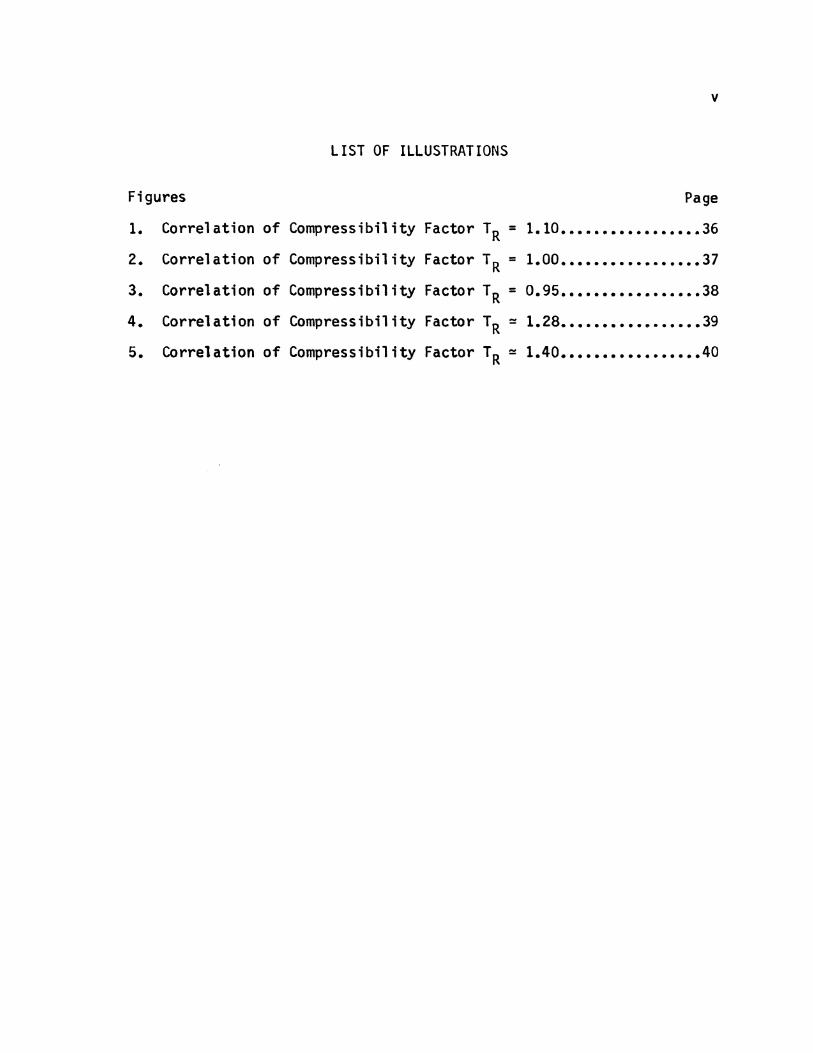
LIST OF ILLUSTRATIONS

Figures Page

1. Correlation of Compressibility Factor T R = 1.10 ......•...•...... 36

2. Correlation of Compressibility Factor T R = 1.00 ......•.......... 37

3. Correlation of Compressibility Factor T R = 0.95 .••.•.•••.....•.. 38

4. Correlation of Compressibility Factor T R = 1.28 •.•...•...•...... 39

5. Correlation of Compressibility Factor TR = 1.40 •••••.•.•..•..••• 40

vi

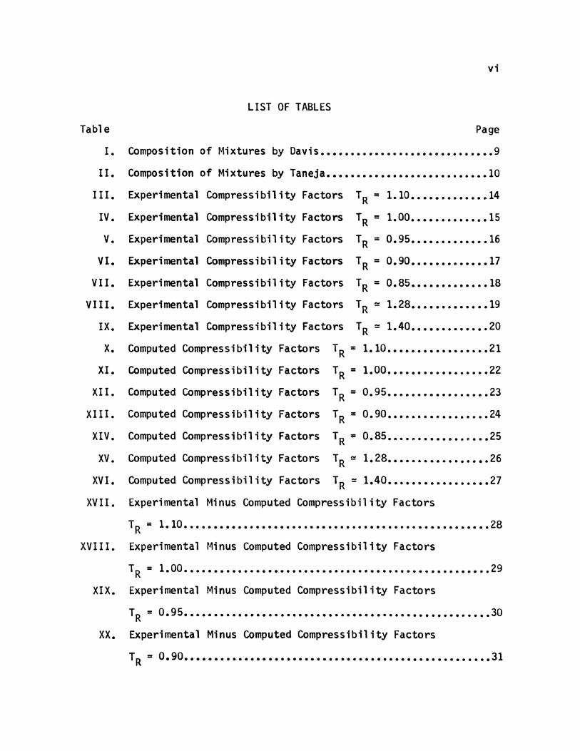
LIST OF TABLES

Table Page

I. Composition of Mixtures by Davis ••••••••••••••••••••••••••••• 9

II. Composition of Mixtures by Taneja ••••••••••••••••••••••••••• lO

I II.

IV.

v. VI.

VII.

VIII.

IX.

x. XI.

XII.

XI II.

XIV.

XV.

XVI.

Experimental Compressibility Factors T = R 1.10 ..•.••..•.•.. 14

Experimental Compressibility Factors T = R 1.00 •••••..•••..• 15

Experimental Compressibility Factors TR = 0.95 ••••..••••••. 16

Experimental Compressibility Factors T = R 0.90 •••••••••.••. 17

Experimental Compressibility Factors TR = 0.85 ••........•.. 18

Experimental Compressibility Factors TR ~ 1.28 ••...•....... 19

Ex peri menta 1 Compressibility Factors TR ~ 1.40 .•••••.•••... 20

Computed Compressibility Factors T = R 1.10 .•.•..••.••...... 21

Computed Compressibility Factors T = R 1.00 .••.••..•••...... 22

Computed Compressibility Factors T = R 0.95 •••••••••••...••. 23

Computed Compressibility Factors T = R 0. 90 • .•• "' ..••••...... 24

Computed Compressibility Factors T = R 0.85 ......••••..... ~.25

Computed Compressibility Factors T -R - 1.28 •......•.....•.•. 26

Computed Compressibility Factors T -R - 1.40 ••.•.••••......•. 27

XVII. Experimental Minus Computed Compressibility Factors

TR = 1.10 ••••••••••••••••••••••••••••••••••••••••••••••••••• 28

XVIII. Experimental f4inus Computed Compressibility Factors

T R = 1. 00 ••••••••••••••••••••••••••••••••••••••••••••••••••• 29

XIX. Experimental Minus Computed Compressibility Factors

TR = 0.95 ••••••••••••••••••••••••••••••••••••••••••••••••••• 30

XX. Experimental Minus Computed Compressibility Factors

TR = 0.90 ••••••••••••••••••••••••••••••••••••••••••••••••••• 31

vii

List of Tables (continued) Page

XXI. Experimental Minus Computed Compressibility Factors

TR = 0.85 •••••.•••.•.••••••.•.••••.••••.•.••.•••••.....••.•. 32

XXII. Experimental Minus Computed Compressibility Factors

TR = 1.28 ••••••••••••••••••••••••••••••••••••••••••••••••••• 33

XXIII. Experimental Minus Computed Compressibility Factors

TR ~ 1.40 ••••••••••••••••••••••••••••••••••••••••••••••••••• 34

XXIV. Critical Temperatures and Pressures of the Mixtures ••••••••• 35

1

I. INTRODUCTION

As the range of operating conditions in the natural gas industry

become more and more varied. the need for prediction of compressibility

factors over a wide range of temperatures and pressures is becoming

more prominent.

The compressibility factors of natural gas mixtures have been

determined by various means. Ill However. certain limitations are

inherent to each of these procedures. 121 Because of these limitations

a more accurate method of predicting compressibility factors has been

sought.

The object of this study is to show that for a natural gas mix

ture. which contains from 2 to 25 mole % nitrogen. it is possible to

predict compressibility factors using the Benedict-Webb-Rubin Equation

of State 131 in conjunction with a correlation graph to correct for

the nitrogen which may be present in the mixture. Various graphs are

presented to correct for the presence of nitrogen. These graphs are

plots of the error in the compressibility factor calculated with the

Benedict-Webb-Rubin Equation of State versus reduced pressure at a

constant reduced temperature with different mole %of nitrogen for

each correction curve.

II. LITERATURE REVIEW

Several methods are available for computing compressibility

factors of hydrocarbon and natural gas mixtures. Ill In a method introduced by Kay Ill • which has the 11 La"' of

Corresponding States, .. as its theoretical basis, the pseudo-reduced

temperature and pressure are assumed to be adequate to predict com

pressibility factors of gaseous hydrocarbon mixtures. Kay introduced

the concept of pseudo-reduced temperature and pseudo-reduced pressure

which are defined mathematically as:

2

pPR = pI pPC

pTR = T I pTe

(1)

where: P and T are absolute pressure and temperature respectively.

and:

n pPC = L Y. p . ;

i=l 1 Cl

n pT = l Y. T .

C i=l 1 Cl

with: pPc =pseudo-critical pressure of the mixture;

( 2)

(3)

(4)

Pci =absolute critical pressure of the individual component;

Tci = absolute critical temperature of the individual component;

pTe = pseudo-critical temperature of the mixture;

Yi = mole fraction of the ith component in the mixture;

n = the number of components in the mixture

Once pPr and pTr are calculated, the compressibility factors may

be determined from graphs prepared by Brown, Katz, Oberfell and Alden.

121 These are standard graphs which the petroleum industry has

universally adopted to determine the compressibility factor for the

equation:

3

PV = ZnRT (5)

These graphs hold only if the mixture is a methane-rich natural gas.

Eilerts stated that the error resulting from nitrogen is less

than 1 % if nitrogen content is less than 10 mole %, less than 3 % if

nitrogen content is less than 20 mole %, and greater than 3 % if more

than 20 mole % nitrogen is present (assuming the Law of Corresponding

States). 121

To compensate for the presence of nitrogen in a hydrocarbon gas,

Eilerts proposed an additive compressibility factor defined as:

za = znyn + (1 - Yn)z9 where:

Zn =compressibility factor of the nitrogen;

Yn = mole fraction of the nitrogen;

Zg = compressibility factor of the hydrocarbon fraction

The true compressibility factor Z is then:

z = cz a

where: C = correction factor dependent of temperature, pressure, and

mo 1 e % nitrogen

Tables are presented l2lto determine the correction factor C.

Various other procedures of correcting for carbon dioxide,

hydrogen sulfide, and water vapor may be found in AmYX 1 Bass, and

Wh 1 t i ng "' 121

In 1940 Benedict, Webb, and Rubin proposed an empirical equation

of state for the phase and volumetric behavior of gases and liquids at

the bubble:.·• point. 131 This equation is a refinement of the Beattie-

Bridgeman Equation of State. The Benedict-Webb-Rubin Equation of

State contains eight empirical coefficients whereas the Beattie

Bridgeman contains only six. The equation developed by Benedict,

4

Webb, and Rubin was guided by several considerations. It is a com

promise between a simple equation and a reasonably accurate descrip

tion of the observed volumetric properties of gases. 131 The coeffi

cients of the equation were based mainly on three main properties; the

volumetric behavior of the gas phase, the prediction of critical pro

perties, and the determination of an accurate vapor pressure. 131

This equation of state does not accurately define the volumetric

behavior of the liquid except at points near the phase boundary of the

substance. This equation is explicit in compressibility factor ana

pressure and the effort to obtain, by reversion, an explicit expression

in molal volume yields an infinite series which is impossible to

develop into any expression of closed form. 131

In a paper presented by Opfell, Sage, and Pitzer 141 the Benedict

Webb-Rubin Equation was applied to the Theorem of Corresponding States.

In this paper, compressibility factors of pure hydrocarbons were com

puted to see if they were applicable to the Theorem of Corresponding

States. The predicted compre~sibility factors were within ± 0.01 of

the experimental values for the pure components. 141

In a paper by Davis, Bertuzzi, Gore, and Kurata a mathematical

technique for predicting critical points of mixtures is presented. 151 This technique for predicting critical points is the one used in this

study. This technique as well as Benedict's equation can be found in

Appendices A, B, and c.

5

III. DISCUSSION

!:.:_ EQUATIONS

.!:.. COMPRESSIBILITY

The equation used to compute compressibility in this study is the

Benedict-Webb-Rubin Equation of State which is:

Z = 1 + (Bo - ~- ~~3 )y-1 + (b - ~)y-2 + nT- y-5

+ ~ v-2 (1 + yV-2) exp (-yv-2) RT.,) • • •

(8)

In order to obtain molal volume for the above equation, another

form of the Benedict-Webb-Rubin Equation of State is used. This

equation is:

where:

-2 B2(T) = BoRT - Ao - CoT ;

Bj(T) = (bRT- a);

B6(T) = aa

(9)

(10)

( 11)

{12)

{13)

The coefficients Ao, Bo, co. a. b. c, a, and y are independent

of temperature and of molal volume.

The pressure equation was solved by a trial and error procedure

(Explained in Appendix A).

6

In order to obtain the coefficients Ao, Bo, Co, a, b, c, ~. and y

the mixing rules proposed by Benedict 161 were used. These rules are:

N Bo = l: n. Bo 1• ( 14)

. 1 1 1=

Ao = D "; (Ao;l~ 2 ( 15). 1

~ N ~ 2 (16) Co = l: n. (Co.) 2

i=1 1 1

~N (b; )1/3] 3 b = l: n. {17) i=1 1

a = l n. ~N i=1 1

(•;ll/~ 3 (18)

c = ~N l: n. =1 1

(c;ll/~ 3 (19)

~ = ~N l n. =1 1

(a;) 1/3] 3 (20)

y = r r n. (y1. )~l 2 G=1 1 J {21)

Where possible, the experimental critical pressure and tempera

ture were used in order to calculate reduced pressure (Pr) and

reduced temperature (Tr).

~ CRITICAL POINTS

When the critical pressure and temperature were not known, the

technique for predicting critical points presented by Davis, Bertuzzi,

Gore, and Kurata was used. 151 This method applies a set of corrections

to the weight average pseudo-critical temperature (mT~) and a set of

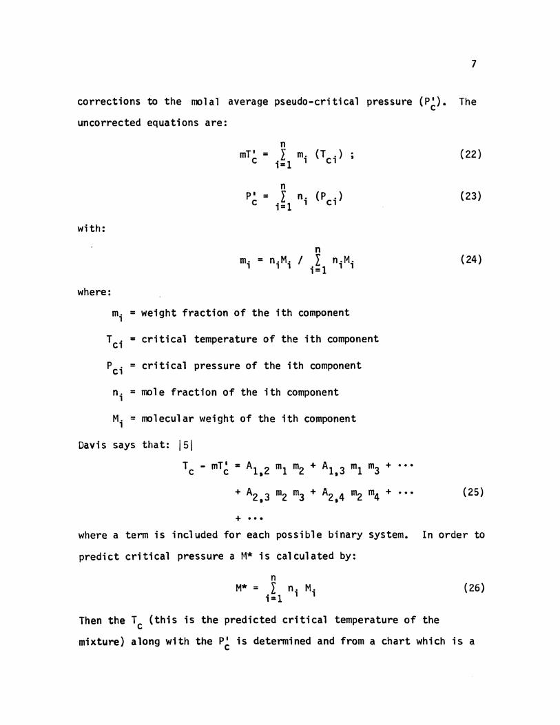
7

corrections to the molal average pseudo-critical pressure (P~). The

uncorrected equations are:

with:

n mT 1 = .I m. (Tci) .

c 1 ' 1=1

n p• = c l n.

i=1 1 (Pci)

n m1. = n1M1. I l n.M.

. 1 1 1 1=

where:

m. = weight fraction of the ith component 1

Tci = critical temperature of the ith component

Pci = critical pressure of the ith component

n1 = mole fraction of the ith component

Mi = molecular weight of the ith component

Davis says that: lSI

Tc - mT~ = A1,2 m1 m2 + A1,3 m1 m3 +

+ A2,3 m2 m3 + A2,4 m2 m4 +

+ •••

(22)

(23)

{24)

...

... (25)

where a term is included for each possible binary system. In order to

predict critical pressure a M* is calculated by:

n M* = l n. M.

i=l 1 1 (26)

Then the Tc (this is the predicted critical temperature of the

mixture) along with the P~ is determined and from a chart which is a

8

plot of Tc P~ I Pc with M* as a parameter, the critical pressure (Pc)

is then calculated.

~ MIXTURES USED IN CORRELATION

The mixtures used in this study were taken from the paper by

Davis. 151 The composition of these mixtures are shown in Table I.

The other mixtures were taken from a Masters Thesis by Mr. P. K.

Taneja. 171 The compositions of these mixtures are shown in Table II.

TABLE I

COMPOSITION OF MIXTURES BY DAVIS j5j

~ A-2 A-3 A-4 AB-2 AB-3 B c 0

Carbon Dioxide, t:1ol e % 1.09 1.00 0.91 0.30 0.20 0.13 0.20 0.25

Helium -- -- -- -- -- 1.00 0.60 0.31

Methane 82.86 76.25 68.70 85.80 73.64 76.65 75.15 85.32

Ethane 4.01 3.69 3.33 1.50 1.20 5.51 6.10 4.11

Propane 1.74 1.60 1.44 0.60 0,53 3.35 3.27 1.98

i-Butane 0.30 0,28 0.30 0.12 0.10 0.35 0,38 0.37

n-Butane 0.55 0.51 0.40 0.18 0.15 0.90 0.60 0.39

i-Pentane 0.19 0.18 0.16 0.06 0.05 0.17 0.20 0.22

n-Pentane 0.12 0.11 0.10 0.04 0.04 0.15 0,20 0.22

Hexanes 0.14 0.12 0.11 0.04 0,04 0.33 0.20 0.22

Heptanes + * 0.16 0.15 0.14 0,06 0.05 0.33 0,20 0.22

Nitrogen 8.84 16.11 24.41 11.30 24.00 11.46 13.50 7.05

*Heptane and higher hydrocarbon components

1.0

TABLE II

COMPOSITION OF MIXTURES BY TANEJA 171

Gas 1 2 3 -Methane, Mole Frac. 0.9707 0.94026 0.9110

Nitrogen 0.0270 0.05528 0.08453

Helium 0.0022 0.004559 0.0043179

4

0.90598

0.08405

0.009967

..... 0

~ METHOD OF CORRELATION

The method of correlation used in this study was to plot devia

tion in computed compressibility factors, using the Benedict-Webb

Rubin equation of state, versus reduced pressure at constant reduced

temperatures for different mole % of Nitrogen.

11

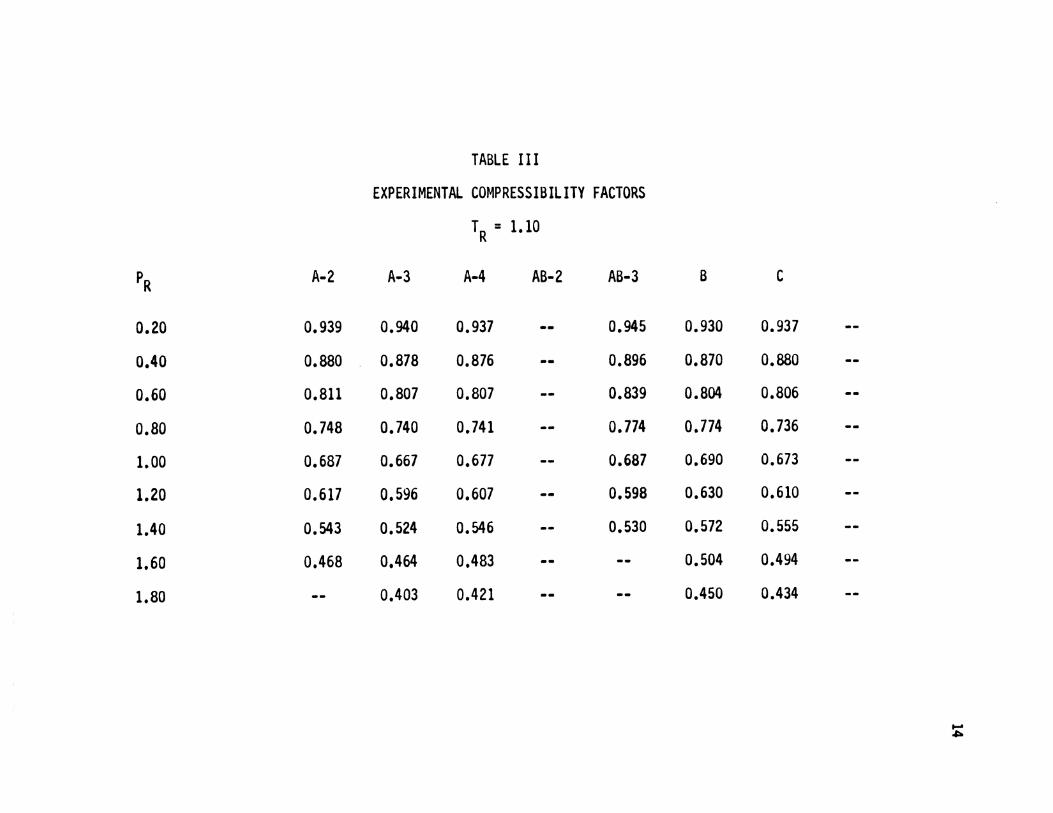
Tables 3 through 7 are taken directly from a paper by Davis. 151

Tables 8 through 9 are taken from a Master•s Thesis by Taneja. 171

Tables 10 through 19 are the result of this study. The -- in the

tables show that no information was available.

12

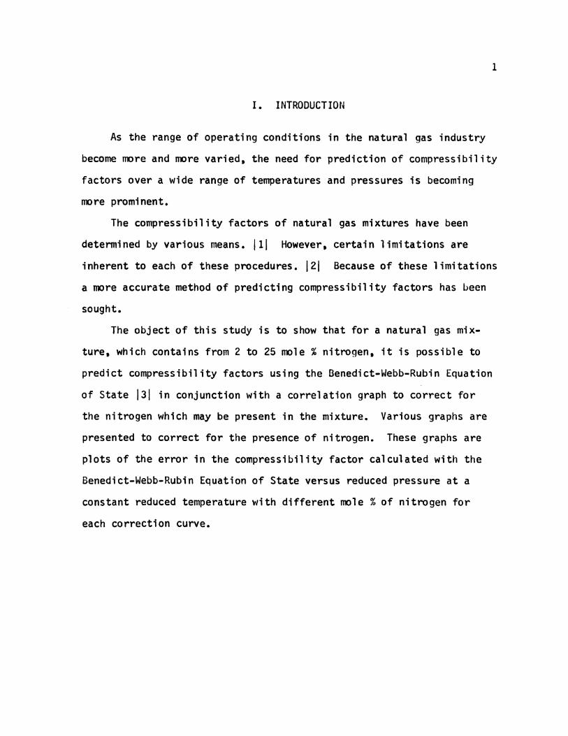
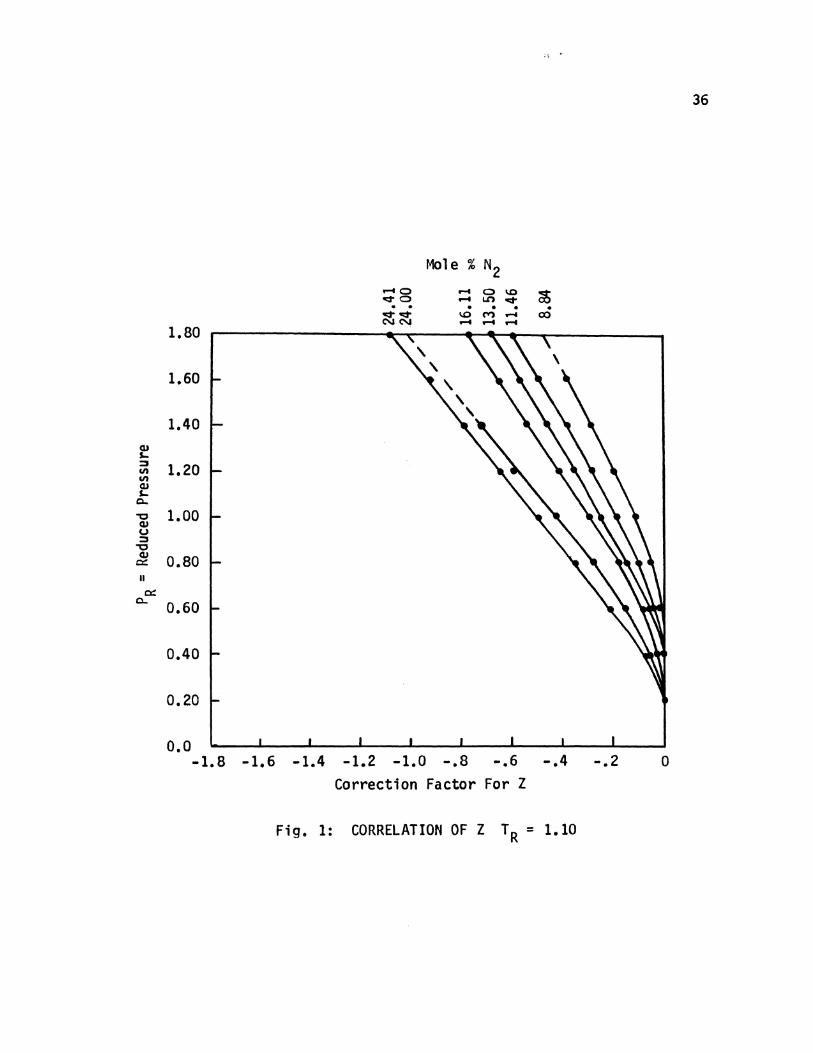
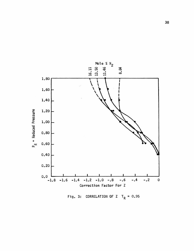
IV. RESULTS

The results of this study are shown in Figures 1-5. In Figures

1 through 3 the results of the deviation versus pressure at different

mole % Nitrogen at constant reduced temperature are shown for the

mixtures presented by Davis. In Figures 4 and 5 the results for the

mixtures presented by Taneja are shown. Because of the closeness of

the critical temperatures the mean was taken as Tc for all mixtures,

(± .85%). In both cases no effort was made to calculate compressi

bilities of any of the mixtures from the graphs, instead; the actual

results are plotted to show the relationship to each other.

Because there is no available data on Carbon Dioxide, as far as

Benedict-Webb-Rubin is concerned, the coefficients for Ethane were

used when Carbon Dioxide was present. IBI Also since there is no coefficient calculated for Helium it was

disregarded in the calculation of compressibility factors. This was

possible because of the small mole% of Helium present in the mixtures

and since the mixing rules for the Benedict-Webb-Rubin are based on a

mole % average.

As can be seen in Figure 3, the correlation is not good for low

values of PR and TR. This is to be expected, because the Benedict

Webb-Rubin equation is not applicable in the two phase region.

Therefore it is not possible to correlate compressibility factors in

that region with this technique.

Although Table XX and Table XXI were not plotted, each table was

prepared to show that the method of correlation used in this study

was not valid in the two phase region.

13

Correlation, in Figures 1 through 3, below values of the critical

temperature and pressure are coincidental and should not be used.

In Figures 4 and 5, Mixture 4 which contains 8.405 mole % of

Nitrogen seems to be out of line. This is probably caused by an

inaccurate prediction of critical pressure. The critical pressure

predicted for Mixture 4 is probably too high and should have been

lower. This would cause the curve to be shifted upwards and also

flattened out. As can be seen, if too high a predicted critical

pressure is actually the case then the two curves of ~1ixture 3 and

Mixture 4 should nearly coincide.

PR A-2

0.20 0.939

0.40 0.880

0.60 0.811

0.80 0.748

1.00 0.687

1.20 0.617

1.40 0.543

1.60 0.468

1.80 --

TABLE III

EXPERIMENTAL COMPRESSIBILITY FACTORS

TR = 1.10

A-3 A-4 AB-2 AB·3

0.940 0.937 -- 0.945

0.878 0.876 -- 0.896

0.807 0.807 -- 0.839

0.740 0.741 -- 0.774

0.667 0.677 -- 0.687

0.596 0.607 -- 0.598

0.524 0.546 -- 0.530

0.464 0.483 -- --0.403 0.421 -- --

B

0.930

0.870

0.804

0.774

0.690

0.630

0.572

0.504

0.450

c

0.937

0.880

0.806

0.736

0.673

0.610

0.555

0.494

0.434

.... •

TABLE IV


T R = 1.00

PR A-2 A-3 A-4 AB-2 AB-3

0.20 0.920 0.912 0.905 0.924 0.911

0.40 0.837 0.825 0.810 0.845 0.829

0.60 o. 742 0.733 0.713 0.750 0.736

0.80 0.622 0.622 0.616 0.618 0.610

1.00 0.460 0.490 0.508 0.427 0.436

1.20 0.322 0.347 0.396 0.286 0.280

1.40 0.240 0.247 0.290 -- --1.60 -- -- -- -- --1.80 -- -- -- -- --

B c

0.910 0.910

0.828 0.820

0.740 0.720

0.646 0.617

0.550 0.509

0.452 0.411

0.370 0.337

0.302 0.302

0.262 0.222

D

0.917

0.830

0.735

0.621

0.485

0.340

0.250

~

0'1

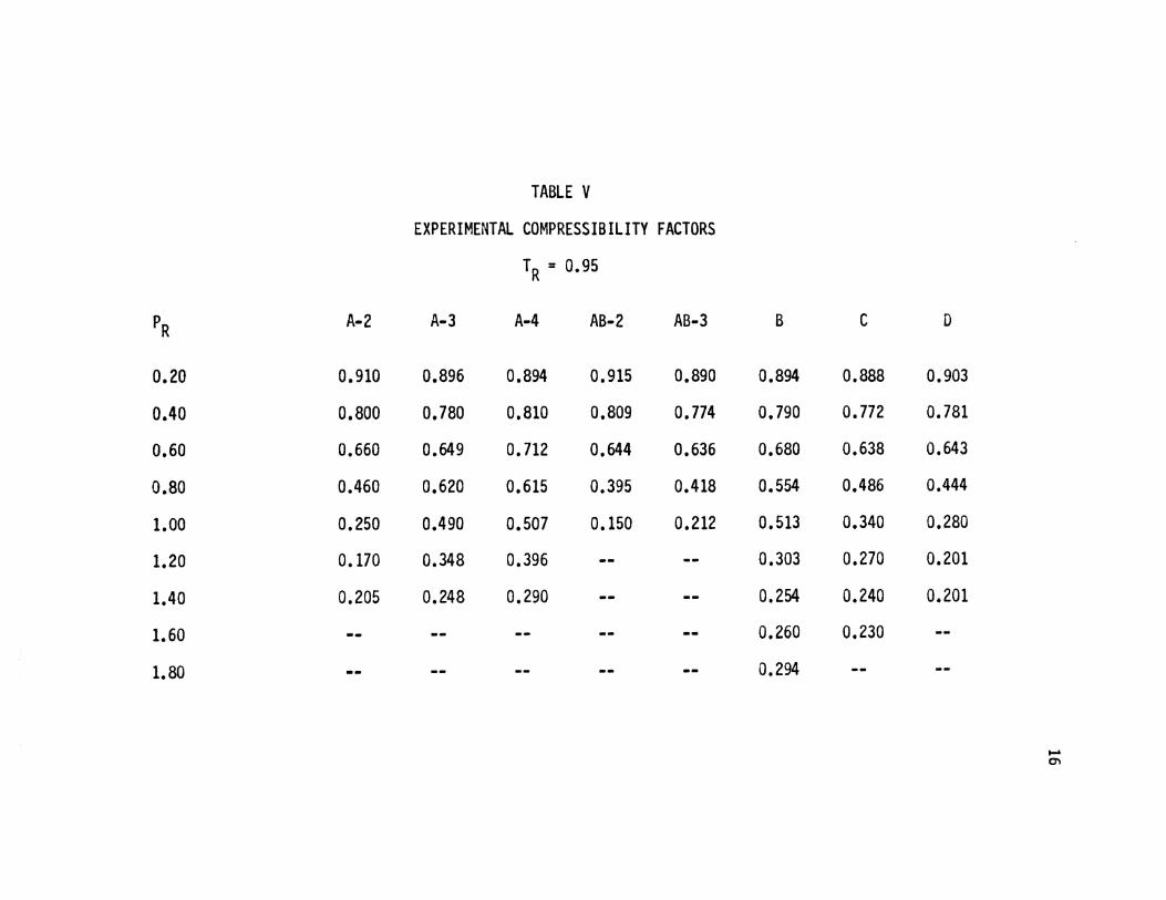
TABLE V


TR = 0.95

PR A-2 A-3 A-4 AB-2 AB-3

0.20 0.910 0.896 0.894 0.915 0.890

0.40 0.800 0.780 0.810 0.809 0.774

0.60 0.660 0.649 0.712 0,644 0.636

0.80 0.460 0.620 0.615 0.395 0.418

1.00 0.250 0.490 0.507 0.150 0.212

1.20 0.170 0.348 0.396 -- --1.40 0.205 0.248 0.290 -- --1.60 -- -- -- -- --1.80 -- -- -- -- --

B c

0.894 0.888

0.790 0.772

0.680 0.638

0.554 0.486

0.513 0.340

0.303 0.270

0.254 0.240

0.260 0.230

0.294

D

0.903

0.781

0.643

0.444

0.280

0.201

0.201

.... 0'1

TABLE VI


TR = 0.90

PR A-2 A-3 A-4 AB-2 AB-3

0.20 0.880 0.877 0.855 0.899 0.860

0.40 0.720 0.694 0.699 0.715 0.690

0.60 0.479 0.470 0.511 0.389 0.421

0.80 0.190 0.245 0.311 -- --1.00 0.134 0.160 0.168 -- --1.20 -- -- -- -- --1.40 -- -- -- -- --1.60 -- -- -- -- --

B

0.855

0.702

0.538

0.390

0.284

0.235

----

c

0.850

0.688

0.505

0.329

0.211

0.180

0.188

0.204

D

0.873

0.706

0.490

0.248

0.162

0.185

0.221

.... ....,

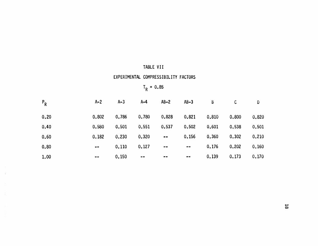
TABLE VII


TR = 0.85

PR A-2 A-3 A-4 AB-2 AB-3

0.20 0.802 0.786 0.780 0.828 0.821

0.40 0.580 0.501 0.551 0.537 0.502

0.60 0.182 0.230 0.320 -- 0.156

0.80 -- 0.110 0.127 -- --1.00 -- 0.150 -- -- --

B c

0.810 0.800

0.601 0.538

0.360 0.302

0.176 0.202

0.139 0.173

D

0.820

0.501

0.210

0.160

0.170

.... co

PR 1

1.184 0.796

1.775 0.706

2.367 0.698

2.959 0.738

3.551 0.806

4.143 0.878

4.734 0.958

5.326 1.058

5.918 1.142

TABLE VIII


TR = 1.28

PR 2 PR 3

1.175 0.782 1.012 0.776

1.762 0.710 1.518 0.697

2.349 0.695 2.024 0.686

2.937 0.732 2.530 0.718

3.524 0.788 3.036 0.780

4.112 0.856 3.542 0.846

4.699 0.930 4.048 0.920

5.286 1.000 4.554 0.998

5.874 1.074 5.059 1.078

PR

1.109

1.664

2.218

2.773

3.327

3.882

4.437

4,991

5.546

4

0.762

0.701

0.694

0.736

0.800

0.871

0.946

1.028

1.104

..... 'Ci

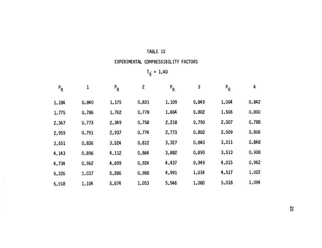
TABLE IX


TR = 1.40

PR 1 PR 2 PR 3

1.184 0.840 1.175 0.831 1.109 0.849

1. 775 0.786 1.762 0.778 1.664 0.802

2.367 0.773 2.349 0.758 2.218 0.790

2.959 o. 791 2.937 0.774 2.773 0.802

3.551 0.836 3.524 0.812 3.327 0.840

4.143 0.896 4.112 0.864 3.882 0.890

4.734 0.962 4.699 0.924 4.437 0.949

5.326 1.037 5.286 0.988 4.991 1,014

5.918 1.104 5.874 1.053 5.546 1.080

PR

1.004

1.506

2.007

2.509

3.011

3.513

4.015

4.517

5.018

4

0.842

0.800

0.788

0.806

0.848

0.908

0.962

1.022

1.094

N 0

TABLE X

C0~1PUTEO COMPRESSIBILITY FACTORS

TR = 1.10

PR A-2 A-3 A-4 AB-2 AB-3

0.20 0.931 0.936 0.949 -- 0.957

0.40 0.871 0.901 0.956 -- 0.957

0.60 0.825 0.899 1.015 -- 0.994

0.80 0.801 0.924 1.091 -- 1.050

1.00 0.798 0.966 1.171 -- 1.118

1.20 0.810 1.013 1.263 -- 1.189

1.40 0.830 1.065 1.345 -- 1.257

1.60 0.861 1.115 1.420 -- --1.80 -- 1.181 1.513 -- --

B

0.920

0.862

0.837

0.844

0.875

0.911

0.954

1.008

1.050

c

0.923

0.873

0.861

0.882

0.919

0.967

1.017

1.062

1.121

D

N .....

TABLE XI

COMPUTED COMPRESSIBILITY FACTORS

T R = 1.00

PR A-2 A-3 A-4 AB-2 AB-3

0.20 0.907 0.916 0.938 0.924 0.947

0.40 0.826 0.880 0.973 0.864 0.963

0.60 0.775 0.896 1.061 0.830 1.026

0.80 0.762 0.945 1.164 0.827 1.108

1.00 0.777 1.008 1.275 0.847 1.197

1.20 0.809 1.079 1.381 0.877 1.290

1.40 0.842 1.148 1.492 -- --1.60 -- -- -- -- --1.80 -- -- -- -- --

B c

0.891 0.896

0.821 0.841

0.810 0.848

0.841 0.891

0.890 0.953

0.946 1.015

1.006 1.092

1.070 1.143

1.131 1.228

D

0.909

0.823

0.756

0.720

o. 718

0.734

0.761

N N

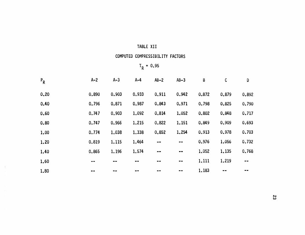
TABLE XII


TR = 0.95

PR A-2 A-3 A-4 AB-2 AB-3

0.20 0.890 0.903 0.933 0.911 0.942

0.40 0.796 0.871 0.987 0.843 0.971

0.60 o. 747 0.903 1.092 0.814 1.052

0.80 0.747 0.966 1.215 0.822 1.151

1.00 0.774 1.038 1.338 0.852 1.254

1.20 0.819 1.115 1.464 -- --1.40 0.865 1.196 1.574 -- --1.60 -- -- -- -- --1.80 -- -- -- -- --

B c

0.872 0.879

0.798 0.825

0.802 0.848

0.849 0.909

0.913 0.978

0.976 1.056

1.052 1.135

1.111 1.219

1.183

D

0.892

0.790

0.717

0.693

0.703

0.732

0.768

N w

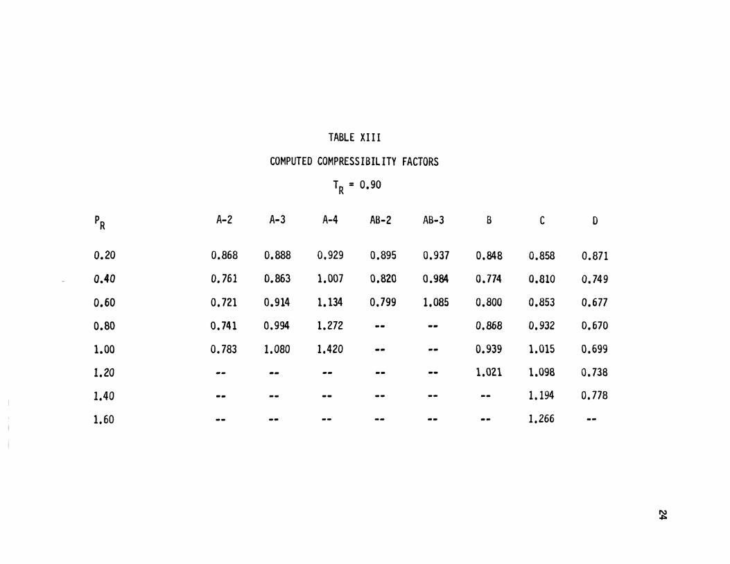
TABLE XIII


TR = 0.90

PR A-2 A-3 A-4 AB-2 AB-3 B c D

0.20 0.868 0.888 0.929 0.895 0.937 0.848 0.858 0.871

0.40 0.761 0.863 1.007 0.820 0.984 0.774 0.810 0.749

0.60 0.721 0.914 1.134 0.799 1.085 0.800 0,853 0.677

0.80 0.741 0.994 1.272 -- -- 0.868 0.932 0.670

1.00 0.783 1.080 1.420 -- -- 0.939 1.015 0.699

1.20 -- -- -- -- -- 1.021 1.098 0.738

1.40 -- -- -- -- -- -- 1.194 0.778

1.60 -- -- -- -- -- -- 1.266

~

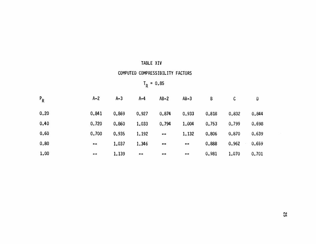
TABLE XIV


TR = 0.85

PR A-2 A-3 A-4 AB-2 AB-3

0.20 0.841 0.869 0.927 0.874 0.933

0.40 o. 720 0.860 1.033 0.794 1.004

0.60 0.700 0.935 1.192 -- 1.132

0.80 -- 1.037 1.346 -- --1.00 -- 1.139 -- -- --

B c

0.818 0.832

0.753 0.799

0.806 0.870

0.888 0.962

0.981 1.070

D

0.844

0.698

0.639

0.659

0.701

N CJl

TABLE XV


TR = 1.28

PR 1 PR 2 PR 3

1.184 0.766 1.175 0.809 1.109 0.852

1.775 0.709 1.762 0.791 1.664 0.867

2.367 0.706 2.349 0.815 2.218 0.914

2.959 0.732 2.937 0.855 2.773 0.956

3.551 0.774 3.524 0.900 3.327 1.032

4.143 0.821 4.112 0.948 3.882 1.092

4.734 0.878 4.699 0.997 4.437 1.146

5.326 0.935 5.286 1.045 4.991 1.202

5.918 0.996 5.874 1.096 5.546 1.253

PR

1.004

1.506

2.007

2.509

3.011

3.513

4.015

4.517

5.018

4

0.854

0.868

0.914

0.971

1.031

1.091

1.147

1.199

1.250

N 0\

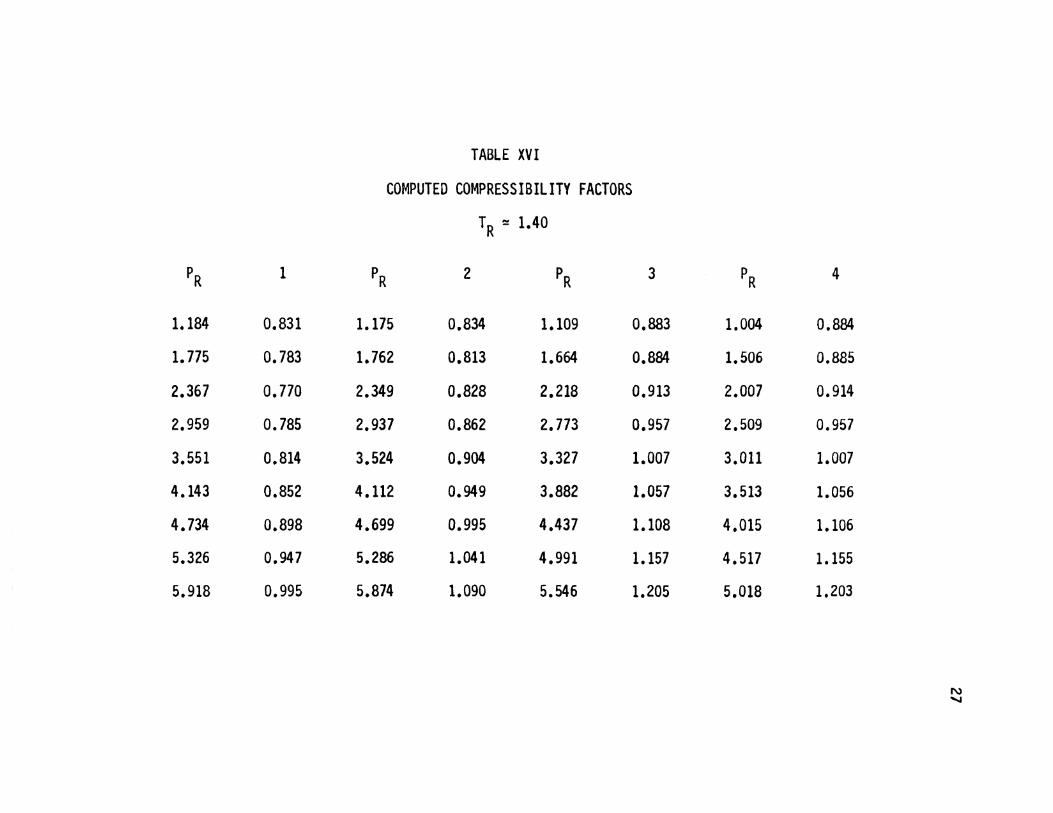
TABLE XVI


TR ~ 1.40

PR 1 PR 2 PR

1.184 0.831 1.175 0.834 1.109

1.775 0.783 1.762 0.813 1.664

2.367 0.770 2.349 0.828 2.218

2.959 0.785 2.937 0.862 2.773

3.551 0.814 3.524 0.904 3.327

4.143 0.852 4.112 0.949 3.882

4.734 0.898 4.699 0.995 4.437

5.326 0.947 5.286 1.041 4.991

5.918 0.995 5.874 1.090 5.546

3 PR

0.883 1.004

0.884 1.506

0.913 2.007

0.957 2.509

1.007 3.011

1.057 3.513

1.108 4.015

1.157 4.517

1.205 5.018

4

0.884

0.885

0.914

0.957

1.007

1.056

1.106

1.155

1.203

1'\) ......

t."i.:' ~ :·, ...

PR

0.20

0.40

0.60

0.80

1.00

1.20

1.40

1.60

1.80

TABLE XVII

EXPERIMENTAL MINUS COMPUTED COMPRESSIBILITY FACTORS

T R = 1.10

A-2 A-3 A-4 AB-2 AB-3 B

+0.006 +0.004 -0.012 -- -0.012 +0.010

+0.009 -0.023 -0.080 -- -0.061 +0.008

-0.014 -0.092 -0.208 -- -0.155 -0.033

-0.053 -0.176 -0.350 -- -0.276 -0.100

-0.111 -0.299 -0.494 -- -0.431 -0.185

-0.193 -0.417 -0.656 -- -0.591 -0.281

-0.287 -0.541 -0.799 -- -o. 121 -0.382

-0.393 -0.651 -0.937 -- -- -0.500

-- -o. 778 -1.092 -- -- -0.600

c

+0.014

+0.007

-0.055

-0.146

-0.246

-0.357

-0.462

-0.568

-0.687

D

N ()0

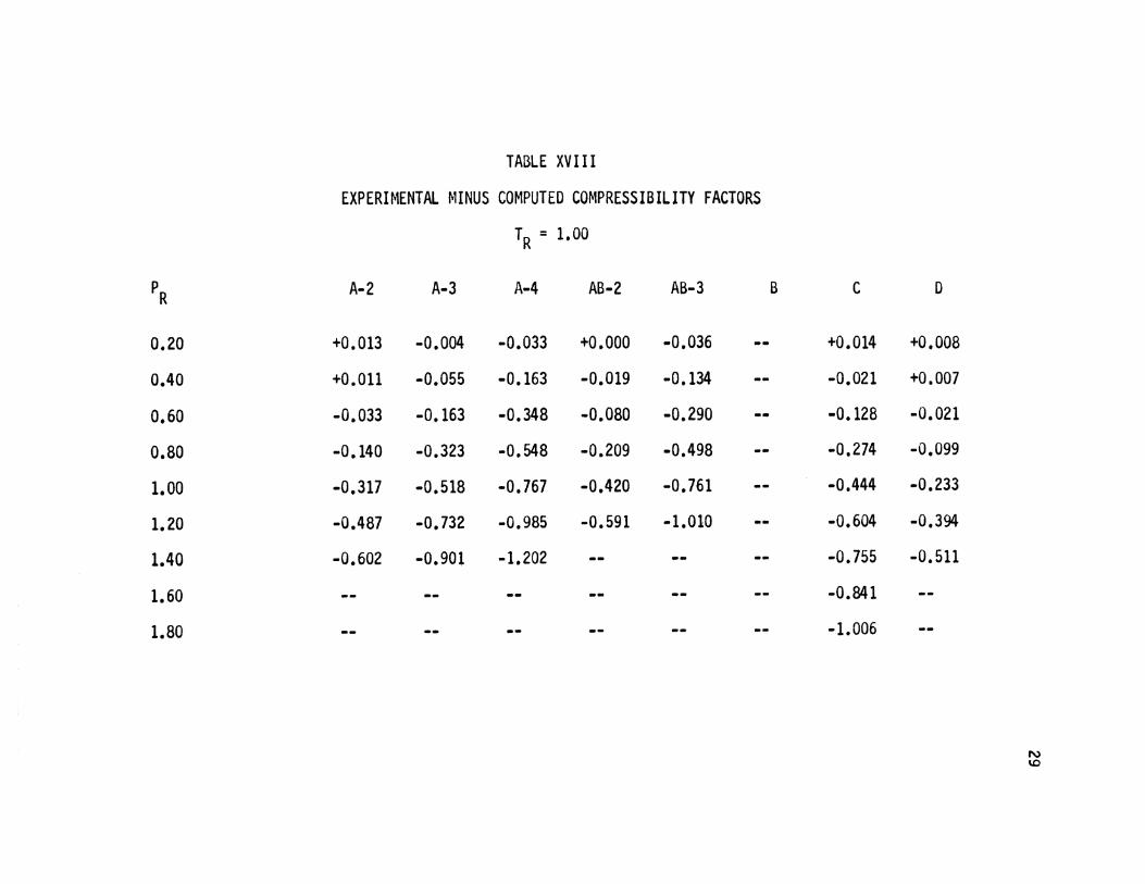
TABLE XVIII


TR = 1.00

PR A-2 A-3 A-4 AB-2 AB-3

0.20 +0.013 -0.004 -0.033 +0.000 -0.036 --0.40 +0.011 -0.055 -0.163 -0.019 -0.134 --0.60 -0.033 -0.163 -0.348 -0.080 -0.290 --0.80 -0.140 -0.323 -0.548 -0.209 -0.498 --1.00 -0.317 -0.518 -0.767 -0.420 -0.761 --1.20 -0.487 -0.732 -0.985 -0.591 -1.010 --1.40 -0.602 -0.901 -1.202 -- .... --1.60 -- -- -- -- -- --1.80 -- -- -- -- -- --

6 c

+0.014

-0.021

-0.128

-0.274

-0.444

-0.604

-0.755

-0.841

-1.006

D

+0.008

+0.007

-0.021

-0.099

-0.233

-0.394

-0.511

N

"'

TABLE XIX


TR = 0.95

PR A-2 A-3 A-4 AB-2 AB-3 B

0.20 +0.020 -0.007 -0.039 +0.004 -0.052 +0.022

0.40 +0.004 -0.091 -0.177 -0.034 -0.197 -0.008

0.60 -0.087 -0.254 i. -0.380 -0.170 -0.416 -0.122

o.8o -0.287 -0.346 -0.600 -0.427 -0.733 -0.295

1.00 -0.524 -0.548 -0.831 -0.702 -1.042 -0.400

1.20 -0.649 -0.767 -1.068 -- -- -0.673

1.40 -0.660 -0.948 -1.284 -- -- -0.798

1.60 -- -- -- -- -- -0.851

1.80 -- -- -- -- -- -0.889

c

+0.009

-0.053

-0.210

-0.423

-0.638

-0.786

-0.895

-0.989

0

+0.011

-0.009

-0.074

-0.249

-0.423

-0.531

-0.567

w 0

TABLE XX


TR = 0.90

PR A-2 A-3 A-4 AB-2 AB-3 B

0.20 +0.012 -0.011 -0.074 +0.004 -0.077 +0.007

0.40 -0.041 -0.169 -0.308 -0.105 -0.294 -0.072

0.60 -0.242 -0.444 -0.623 -0.410 -0.664 -0.262

0.80 -0.551 -o. 749 -0.961 -- -- -0.478

1.00 -0.649 -0.920 -1.252 -- -- -0.655

1.20 -- -- -- -- -- -0.786

1.40 -- -- -- -- -- --1.60 -- -- -- -- -- --

c

-0.008

-0.122

-0.348

-0.603

-0.804

-0.918

-1.006

-1.062

D

+0.002

-0.043

-0.187

-0.422

-0.537

-0.553

-0.557

w ....

TABLE XXI


T R = 0.85

PR A-2 A-3 A-4 AB-2 AB-3 B

0.20 -0.039 -0.083 -0.147 -0.046 -0.112 -0.008

0.40 -0.140 -0.359 -0.482 -0.257 -0.502 -0.152

0.60 -0.518 -0.705 -0.872 -- -0.976 -0.446

0.80 -- -0.927 -1.219 -- -- -0.712

1.00 -- -0.989 -- -- -- -0.842

c

-0.032

-0.261

-0.568

-0.760

-0.897

D

-0.024

-0.197

-0.429

-0.499

-0.531

w 1\l

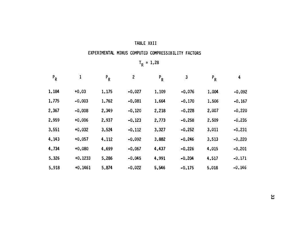
TABLE XXII


TR :: 1.28

PR 1 PR 2 PR 3

1.184 +0.03 1.175 -0.027 1.109 -0.076

1.775 -0.003 1.762 -0.081 1.664 -0.170

2.367 -0.008 2.349 -0.120 2.218 -0.228

2.959 +0.006 2.937 -0.123 2.773 -0.258

3.551 +0.032 3.524 -0.112 3.327 -0.252

4.143 +0.057 4.112 -0.092 3.882 -0.246

4.734 +0.080 4.699 -0.067 4.437 -0.226

5.326 +0.1233 5.286 -0.045 4.991 -0.204

5.918 +0.1461 5.874 -0.022 5,546 -0.175

PR

1.004

1.506

2.007

2.509

3.011

3.513

4.015

4.517

5.018

4

-0.092

-0.167

-0.220

-0.235

-0.231

-0.220

-0.201

-0.171

-0.146

w w

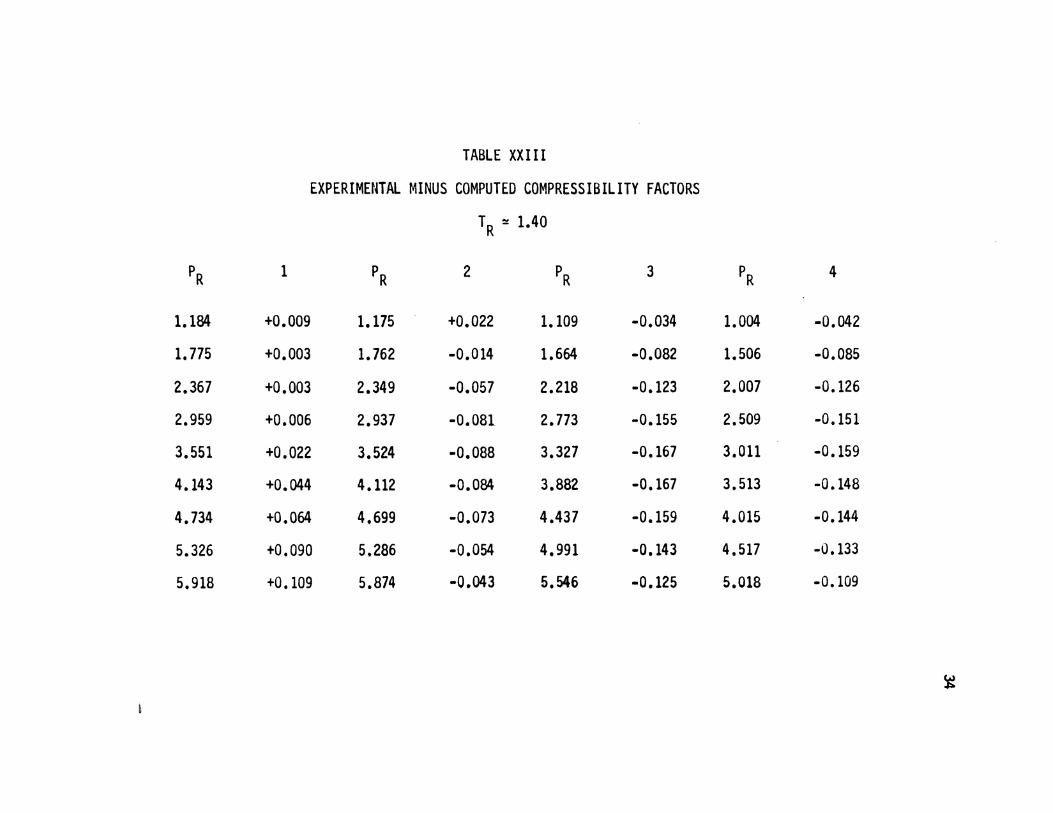
TABLE XXIII


TR = 1.40

PR 1 PR 2 PR 3 PR 4

1.184 +0.009 1.175 +0.022 1.109 -0.034 1.004 -0.042

1.775 +0.003 1.762 -0.014 1.664 -0.082 1.506 -0.085

2.367 +0.003 2.349 -0.057 2.218 -0.123 2.007 -0.126

2.959 +0.006 2.937 -0.081 2.773 -0.155 2.509 -0.151

3.551 +0.022 3.524 -0.088 3.327 -0.167 3.011 -0.159

4.143 +0.044 4.112 -0.084 3.882 -0.167 3.513 -0.148

4.734 +0.064 4.699 -0.073 4.437 -0.159 4.015 -0.144

5.326 +0.090 5.286 -0.054 4.991 -0.143 4.517 -0.133

5.918 +0.109 5.874 -0.043 5.546 ·0.125 5.018 -0.109

~

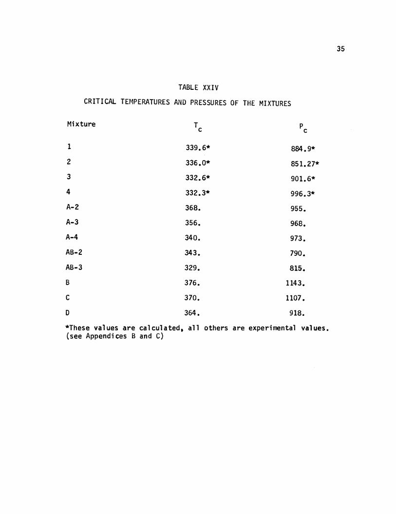
TABLE XXIV

CRITICAL TEMPERATURES AND PRESSURES OF THE MIXTURES

Mixture T p c c

1 339.6* 884.9*

2 336.0* 851.27*

3 332.6* 901.6*

4 332.3* 996.3*

A-2 368. 955.

A-3 356. 968.

A-4 340. 973.

AB-2 343. 790.

AB-3 329. 815.

B 376. 1143.

c 370. 1107.

D 364. 918.

*These values are calculated, all others are experimental values. (see Appendices B and C)

35

36

Mole % N2 .-40 - 0 1.0 ~ q-O -Lt) q-. . . • • . ~~ 1.0 M .-4 00 ---1.80

1.60

1.40 <IJ s.. :::::1 1.20 en en <IJ s..

Q..

"C 1.00 <IJ u :::::1

"C <IJ 0.80 ex II

ex Q..

0.60

0.40

0.20

o.o -1.8 -1.6 -1.4 -1.2 -1.0 -.8 -.6 -.4 -.2 0

Correction Factor For z

Fig. 1: CORRELATION OF Z TR = 1.10

o.o

LO 0 . "'

-1.8 -1.6 -1.4 -1.2 -1.0 -.8 -.6 -.4 -.2 0 Correction Factor For Z


37

38

Mole % N2 ..... 0 \0 tS ..... Ln od" . . . . \0 M ..... co ..... ..... .....

1.80

1.60

1.40

cv 1.20 s-:s Ill Ill

~ 1.00 Q.

'"0 cv (,J :s 0.80 '"0 cv ex: II

ex: 0.60 Q.

0.40

0.20

o.o -1.8 -1.6 -1.4 -1.2 -1.0 -.8 -.6 -.4 -.2 0

Correction Factor For Z


39

Mole% N2 M In co In 0 N 0 .q .q In ....... . . . . co co In N

6.0

5.0

4.0

f :::J lit lit 3.0 (lJ

'-c.. ~ (lJ u :::J

"'tJ Ql

c:z::: II 2.0

c:z::: c..

1.0

0.0~--~--~~--~--~----~--_. ____ ._ __ _. __ ~ -.30 -.25 -.20 -.15 -.10 -.05 0 0.05 0.10 0.15



cu s.. :::1

"' en QJ s..

c... "'0 cu u :::1

"'0 QJ

0:::

II

0::: c...

6.0

5.0

4.0

3.0

2.0

1.0

o.o

M 1.0 "d" . 00

00 N L.O

-.30 -.25 -.20 -.15 -.10 -.05 0 0.05 0.10 0.15


Fig. 5: CORRELATION OF Z TR ~ 1.40

40

41

V. CONCLUSIONS AND RECOMMENDATIONS

The investigation of the varying hydrocarbon systems presented in

this study would tend to indicate that Helium's effect on the compress

ibility factors of these mixtures is to raise the critical point and

that should the critical points of a mixture be known it would then be

possible to predict compressibility factors of mixtures which contain

nitrogen by use of the Benedict-Webb-Rubin equation and a correction

graph for nitrogen. This study seems to indicate that as soon as it

is possible to predict critical points more accurately than is now

possible that charts may be drawn to correlate compressibility factors

over a wide range o~ temperatures and pressures.

It would be interesting to tabulate and study a wide variety of

binary systems to see if a mixing rule as proposed by Lorentz 131 could be used to correct the Benedict-Webb-Rubin equation directly.

If this were possible then most compressibility factors could be cal

culated with one basic equation.

Also a refinement of the method of predicting critical points

used in this study might be found to predict critical points more

accurately.

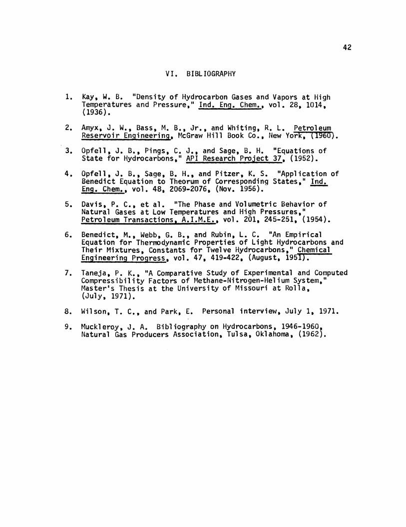
VI. BIBLIOGRAPHY

1. Kay, W. B. 11 Density of Hydrocarbon Gases and Vapors at High Temperatures and Pressure," Ind. Eng. Chern., vol. 28, 1014, (1936).

2. Amyx, J. W., Bass, M. B., Jr., and Whiting, R. L. Petroleum Reservoir Engineering, McGraw Hill Book Co., New York, (196o}.

3. Opfell, J. B., Pings, c. J., and Sage, B. H. 11 Equations of State for Hydrocarbons, .. API Research Project 37, (1952).

4. Opfell, J. B., Sage, B. H., and Pitzer, K. s. 11Application of Benedict Equation to Theorum of Corresponding States, .. Ind. Eng. Chern., vol. 48, 2069-2076, (Nov. 1956). ----

5. Davis, P. c., et al. "The Phase and Volumetric Behavior of Natural Gases at Low Temperatures and High Pressures, .. Petroleum Transactions. A.I.M.E., vol. 201, 245-251, (1954).

42

6. Benedict, M., Webb, G. B., and Rubin, L. C. "An Empirical Equation for Thermodynamic Properties of Light Hydrocarbons and Their Mixtures, Constants for Twelve Hydrocarbons," Chemical Engineering Progress, vol. 47, 419-422, (August, 1951).

7. Taneja, P. K., "A Comparative Study of Experimental and Computed Compressibility Factors of Methane-Nitrogen-Helium System, .. Master's Thesis at the University of Missouri at Rolla, (July, 1971}.

B. Wilson, T. c., and Park, E. Personal interview, July 1, 1971.

9. Muckleroy, J. A. Bibliography on Hydrocarbons, 1946-1960, Natural Gas Producers Association, Tulsa, Oklahoma, {1962).

43

VII. VITA

Terry Wayne Buck was born May 23, 1948 in Kennett. Missouri. He

received his primary and secondary education in Hornersville, Missouri

and in Senath, Missouri. He enrolled in the University of Missouri at

Rolla in September 1966. He received a Bachelor of Science degree in

Petroleum Engineering in August of 1970.

He has been enrolled in the Graduate School of the University of

Missouri at Rolla since September of 1970.

44

VIII. APPENDICES

APPENDIX A

SAMPLE CALCULATION FOR C0~1PRESSIBILITY FACTORS

First the coefficients of the Benedict-Webb-Rubin Equation of

State must be calculated.

Bo was calculated in the following way with the other seven

coefficients calculated similarly:

n

45

Bo= l n.Bo. i=1 1 1

(A-1)

with:

n = number of components

ni = mole fraction of the nth component

Boi = individual coefficient for that particular component

CALCULATION OF Bo FOR MIXTURE 1

n = 3

"1 = .9707 (Hethane)

n = 2 .0270 (Nitrogen)

n3 = .0022 (Hel i urn)

Since Helium was disregarded in Calculation of Compressibility

factor Bo 3 = 0.0 (Helium)

Bo 1 = 0.682401 (Methane)

Bo2 = 0.733661 (Nitrogen)

Bo = (0.682401) {0.9707) + 0.733661 (0.0270) + o.o (0.0022)

Bo = .682215

46

Next a molal volume must be calculated to use in the calculation

of compressibility factor. The equation in P was used with a trial

and error procedure on V: •

P = B1(T)/y + B2(T)ty 2 + Bj(T}ty3 + a6(T)/y 6

+ c/V3T2 (1 + yV-2) exp (-yv-2) . . . where:

a1 (T) = RT;

B2(T) = BaRT -Ao -CoT-2;

B3{T) = {bRT -a);

a6(T) = aa

and:

(A-2)

(A-3)

(A-4)

(A-5)

(A-6)

Ao, Bo, Co, b, c, a, and y = Benedict-Webb-Rubin coefficients

For a set P and T, a V is assumed to be 0.5 then P is calculated •

from the above equation. If the Pcalc.<calculated) is greater than

the Pset an increment of 0.005 is added to y and a new P is calculated

and so on until Peale. is less than Pset and that volume is used for

the compressibility equation. The computer was used to calculate this

pressure.

~XAMPLE CALCULATION OF MOLAL VOLUME OF MIXTURE 1 WITH P = 1000. psig

AND T = 470° R

Ao = 6888.60

Bo = 0.682215

Co = 267,276,000.

c = 723,527,000.

b = 0.849957

a = 2885.03

a. = 1. 54237

y = 0.521307

An example of computer output for different values of V is: . Assume V = 0.5

•

From Equation (A-2)

81(470) = 5044.70

82(470) = -4656.94

83(470) = 1402.79

86(470) = 4449.78

p = 299.517

Because Peale. is greater than Pset• a new value is selected by the

computer.

v = 0.505 . Peale. = 280.928.

and •••

Until V ,., 4.130 •

Peale. = 1015.75 psia

Peale. is greater than Pset

So V = 4.135 •

P = 1014.68 psia

p 1 is less than P ca c. set

Use V = 4.135 for compressibility factor calculation .

47

48

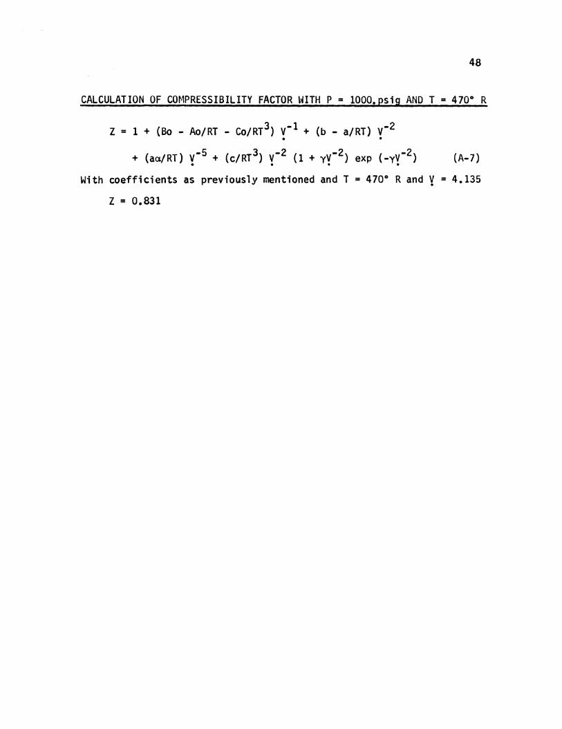
CALCULATION OF COt4PRESSIBILITY FACTOR \HTH P = 1000. psig AND T = 470° R

Z = 1 + (Bo - Ao/RT - Co/RT3) v- 1 + {b - a/RT) v-2 • •

With coefficients as previously mentioned and T = 470° Randy = 4.135

z = 0.831

APPENDIX B

SAMPLE CALCULATION OF CRITICAL TEMPERATURES

FOR MIXTURES 1 THROUGH 4

For calculation of critical temperature the weight average

critical temperature (mT~) was first calculated:

n

49

mT 1 = I m. T . C i= 1 1 Cl

(B-1)

where:

n = number of components.

m = mass fraction of individual component

Tci = critical temperature of individual component

with mi defined as:

where:


x1 = mole fraction of individual component

M1 = molecular weight of individual component

CALCULATION OF WEIGHT AVERAGE CRITICAL TEMPERATURE FOR MIXTURE

Component X M xM m T 0 R c

c1 0.9707 16.04 15.57 0.9529 343.4

N2 0.0270 28.02 0.76 0.0465 227.0

He 0.0022 4.00 0.01 0.0006 9.45

(B-2)

1

mT c 327.2

10.6

16.34 1.0000 mT • = 337.8 c

Next a correction factor was applied to the weight average

critical temperature according to:

Tc - mT~ = A1,2 m1 m2 + A1,3 m1 m2 + ... + A2,3 m2 m3 + A2,4 m2 m4 + •••

... + •••

where:

Tc = corrected critical temperature

A1, 2• A1,3• A2, 3• ••• = correction factor read from the

literature lSI CALCULATION OF CRITICAL TEMPERATURE FOR MIXTURE

m

c1 0.9529

r~2 He 0.0006

(N2)

c1 He 0.0006

(Cl)

T = mT 1 + 1 8 c c •

T = 337.8 + 1.8 = 339.6° R c

A

41.0

Not Given

0.0465 X

Not Given

0.9529 X

1

rnA

39.1

... 39.1 = + 1.8

...

... = ... + 1.8

50

(B-3)

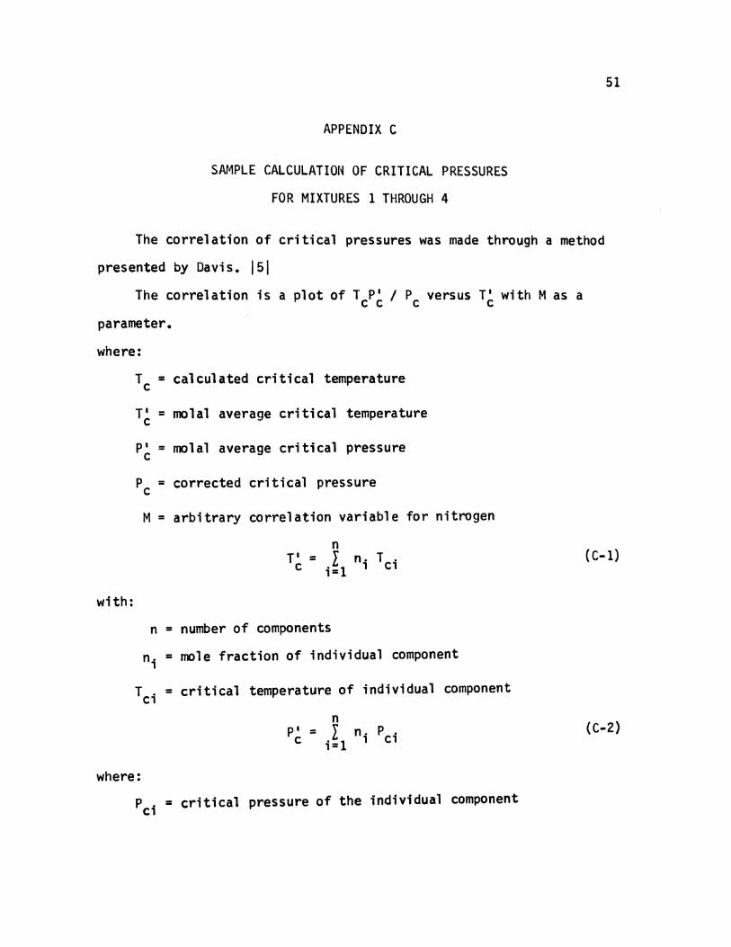
APPENDIX C

SAMPLE CALCULATION OF CRITICAL PRESSURES

FOR MIXTURES 1 THROUGH 4

51

The correlation of critical pressures was made through a method

presented by Davis. lSI The correlation is a plot of TcP~ I Pc versus T~ with Mas a

parameter.

where:

with:

Tc = calculated critical temperature

T' = molal average critical temperature c

P' = molal average critical pressure c

PC = corrected critical pressure

M = arbitrary correlation variable for nitrogen

n T' = I n. T .

C i=l 1 C1


ni = mole fraction of individual component

Tci = critical temperature of individual component

n P' = I c i=l

n. P • 1 C1

where:

Pci =critical pressure of the individual component

(C-1)

(C-2)

52

n M* = l n. Mi

i=1 1 {C-3)

where:

Mi = molecular weight of the individual component

Once Tc• Pc• M, and T~ are calculated TcP~ I Pc is read off of

the graph and Pc is calculated by:

Pc = (Value off of graph) (Tc P~)

In order to account for helium 100 psi is added to the calculated

critical pressure for each mole %of helium present.

CALCULATION OF CRITICAL PRESSURE FOR MIXTURE 1

T = 339.6° R c

P' = 0.9707 (673) + 0.0270 {491) + 0.006 (33.2) c

P' = 666.7 c

T' = 0.9707 (343.4) + 0.0270 (227) + 0.006 (9.45) c

T' = 339.49 c

M = 16.34

T P' I P = 339.49 (666.7) I Pc = 275 c c c

p = 822.9 + 22 (correction for Helium) c

P = 844.9 psia c

53

IX. NOMENCLATURE

Ao,Bo,Co,a,b,c,a, and y = Benedict-Webb-Rubin coefficients

c

M*

mT' c

= Correction factor dependent on temperature,

pressure, and mole %nitrogen

= Arbitrary correlating number

= Weight average pseudo-critical temperature

=Molecular weight of ith component

= Absolute pressure, psia

= Mole average pseudo-critical pressure

= Absolute critical pressure of the ith campo-

nent

= Pseudo-reduced pressure

= Universal Gas Law constant

= Absolute temperature, oR

= Corrected critical temperature

= Mole average pseudo-critical temperature

= Absolute critical temperature of the ith

component

= Pseudo-reduced temperature

= Volume

= Specific volume

= t-1ol e fraction of i th component

= ~Dle fraction of nitrogen component

= Compressibility factor

=Additive compressibility factor

=Compressibility factor for hydrocarbon

component

=Compressibility factor for nitrogen

component

= Mass fraction of ith component

= Number of components in the mixture

= Mole fraction of ith component

54

an empirical method of correlating compressibility factors

Documents