an empirical study of cache-oblivious polygon indecomposability testing

Computing (2010) 88:55–78DOI 10.1007/s00607-010-0086-z

An empirical study of cache-oblivious polygonindecomposability testing

Fatima K. Abu Salem · Rawan N. Soudah

Received: 1 December 2009 / Accepted: 1 March 2010 / Published online: 24 March 2010© Springer-Verlag 2010

Abstract We implement and undertake an empirical study of the cache-obliviousvariant of the polygon indecomposability testing algorithm of Gao and Lauder, basedon a depth-first search (DFS) traversal of the computation tree. According to AbuSalem, the cache-oblivious variant exhibits improved spatial and temporal localityover the original one, and its spatial locality is optimal. Our implementation revolvesaround eight different variants of the DFS-based algorithm, tailored to assess the trade-offs between computation and memory performance as originally proposed by AbuSalem. We analyse performance sensitively to manipulations of the several parame-ters comprising the input size. We describe how to construct suitably random familiesof input that solicit such variations, and how to handle redundancies in vector com-putations at no asymptotic increase in the work and cache complexities. We reportextensively on our experimental results. In all eight variants, the DFS-based variantachieves excellent performance in terms of L1 and L2 cache misses as well as totalrun time, when compared to the original variant of Gao and Lauder. We also bench-mark the DFS variant against the powerful computer algebra system MAGMA, in thecontext of bivariate polynomial irreducibility testing using polygons. For sufficientlyhigh degree polynomials, MAGMA either runs out of memory or fails to terminateafter about 4 h of execution. In contrast, the DFS-based version processes such input

Communicated by C. C. Douglas.

The first author was supported by LNCSR grant 111135-522312 and AUB-URB grant 111135-988119.

F. K. Abu Salem (B) · R. N. SoudahComputer Science Department, American University of Beirut,P. O. Box 11-0236, Riad El Solh Beirut 1107 2020, Lebanone-mail: [email protected]

R. N. Soudahe-mail: [email protected]

123

56 F. K. Abu Salem, R. N. Soudah

using a couple of seconds. Particularly, we report on absolute irreducibility testing ofbivariate polynomials of total degree reaching 19,000 in about 2 s for the DFS variant,using a single processor.

Keywords Computer algebra · Multivariate and bivariate polynomials · Absoluteirreducibility testing · Newton polytopes · Cache-oblivious algorithms · Performanceevaluation

Mathematics Subject Classification (2000) 11R09 · 33F10 · 11Y16 · 68M20 ·91E45

1 Introduction

Recently, algorithm designers have been faced with an increasingly growing proces-sor/memory performance gap that they need to address in order to achieve scalableperformance and improve on resource usage. For this, one must reduce the effects ofthe underlying memory hierarchy, especially in the case of memory intensive applica-tions, by minimising their input/output (I/O) latency. This long established but recentlyappreciated trend recognises the importance of both computation and memory per-formance overhead of algorithms, and carves the proper trade-offs between them.Algorithms tuned in this respect can be either cache-aware [4] or cache-oblivious[8]. Both paradigms result in algorithms with improved memory performance, butcache-aware designs require knowledge of, and thus tuning cache parameters. Cache-oblivious algorithms do not, and are thus more elegant and portable, eliminating theneed for programmer intervention.

In this context, we address the cache-oblivious reformulation in Ref. [2] of thepolygon indecomposability testing algorithm of Ref. [11]. Given a positive integern ≥ 2 and a polytope P as a list of vertices in Z

n , consider the associated questionwhether or not P decomposes into two non-trivial polygons with vertices in N

n . InRef. [11], this problem is shown to be NP-complete, and a pseudo-polynomial timealgorithm for testing polygon indecomposability is obtained. When associated withabsolute irreducibility testing of bivariate and multivariate polynomials over arbitraryfields, the resulting test is considerably faster than many existing irreducibility testingalgorithms, such as in Refs. [7,10,25,13,15,16]. Some more desirable implicationsof polygon indecomposability testing in the context of absolute irreducibility testingis that when decisive, this association can help test families of polynomials, or onegiven polynomial viewed over infinitely many fields. In Ref. [2], a cache-obliviousvariant of the algorithm in Ref. [11] is obtained based on a depth-first search (DFS)traversal of the computation tree, and show that the cache-oblivious variant exhibitsimproved spatial and temporal locality over the original one, and that its spatial localityis optimal. Preliminary tests indeed confirm a non-trivial improvement in practice.

This paper is complementary to the work in Ref. [2] in the following respects. Thecache-oblivious model, also known as the ideal cache model, imposes several assump-tions that are sometimes deemed too simplistic. For example, the ideal cache modelreasons about a hierarchy consisting only of two levels, with the cache operating under

123

An empirical study of cache-oblivious polygon indecomposability testing 57

full associativity, optimal replacement policy, and automatic replacement (see Ref. [8]for more details). Despite that both cache-aware and cache-oblivious designs mayyield the same asymptotic bounds on the cache complexity of any one given problem,the strong assumptions imposed by the cache-oblivious model make it more urgingto address its usefulness in practice and to verify that cache oblivious designs arereasonably efficient when implemented on real caches. The kind of experimentationand performance analysis presented here constitute an essential part for assessing theusefulness of the theoretical study presented in Ref. [2].

We implement the DFS-based cache oblivious variant and instrument it using thePerformance Application Programming Interface (PAPI). Our primary goal is in test-ing the trade-offs put forward in Ref. [2], balancing computation and memory accesses.For this, our implementation revolves around eight different variants of the DFS-basedalgorithm, tailored to assess these trade-offs. We analyse performance sensitively tomanipulations in the several parameters comprising the input size. We describe indetail how to construct suitably random families of input that solicit such variationsand how to handle redundancies in vector computations at no asymptotic increase inthe work and cache complexities. We report extensively on our experimental results.In all eight variants, the DFS-based variant achieves excellent performance in termsof L1 and L2 cache misses as well as total run time, when compared to the originalvariant in Ref. [11]. We also benchmark the DFS variant against MAGMA in thecontext of bivariate polynomial irreducibility testing using polygons. For sufficientlyhigh degree polynomials, MAGMA either runs out of memory or fails to terminateafter about 4 h of execution. In contrast, the DFS-based version processes such inputusing a couple of seconds. Particularly, we report on absolute irreducibility testing ofbivariate polynomials of total degree reaching 19,000 in about 2 s for the DFS variant,using a single processor.

2 Background

2.1 The ideal cache model [8]

The ideal cache model delivers cache-oblivious algorithms. The model reasons abouta data cache consisting of only two levels of memory, labeled as cache and mainmemory. It assumes full associativity of cache, an optimal replacement policy—todecide on which cache blocks get evicted to make room for others— and an automaticreplacement policy—to decide on how cache blocks get replaced in cache. The modelreasons about both the work and cache complexity, the latter being defined as the totalnumber of I/O’s; i.e. words transferred between cache and main memory.

2.2 Polygon indecomposability and polynomial irreducibility testings

Higher dimensional polytope indecomposability testing can be achieved proba-bilistically by performing a number of deterministic polygon indecomposabilitytestings, as described in Ref. [11]. We thus restrict our attention to polygons in Z

2

123


and associated bivariate polynomials. Let P denote a convex polygon with m verticesin Z

2, so that we speak of an integral polygon. Consider the vertices v0, . . . , vm−1 ofP ordered cyclically in a counter-clockwise direction around a chosen pivot, say v0.The pivot may be chosen as the lowest leftmost vertex of the convex polygon. Theedges of P are expressed as vectors of the form Ei = v(i+1) mod m − vi = (ai , bi ),for all i = 0, . . . , m − 1, and where ai , bi ∈ Z. An edge vector Ei is said to beprimitive if gcd(ai , bi ) = 1. Let ni = gcd(ai , bi ) and ei = (ai/ni , bi/ni ). ThenEi = ni ei , where ei is a primitive vector. Each edge vector Ei contains exactlyni + 1 integral points including its end points. The edge sequence of P given by thevectors {ni ei }0≤i≤m−1 uniquely identifies the polygon up to translation determinedby v0. The edge vectors of P form a closed path, so that

∑0≤i≤m−1 ni ei = (0, 0).

For convenience, an edge sequence can be identified with that obtained by extend-ing the sequence by inserting an arbitrary number of zero vectors. This makesit possible to assume that the edge sequence of a summand of P has the samelength as that of P . Gao and Lauder’s polygon indecomposability testing algo-rithm checks for the existence of an arbitrary non-trivial summand of P , whichmust have an edge sequence of the form

∑0≤i≤m−1 ki ei , where 0 ≤ ki ≤ ni ,

ki �= 0 for at least one i , and ki �= ni for at least one i . The algorithm is givenbelow:

Algorithm 1 [11] Input: The edge sequence {ni ei }0≤i≤m−1 of an integral convex

polygon P where ei ∈ Z2 are primitive vectors, and a chosen pivot v0.

Output: Whether P is decomposable.

Step 1: Compute the set of all the integral points in P. Also make use of this set toanswer queries on whether arbitrary points in the plane belong to P. Set A−1 = ∅.Step 2: For i = 0, . . . , m − 2, compute the set of points in P that are reachable viathe vectors e0, . . . , ei :

2.1: For each k = 1, . . . , ni , if v0 + kei ∈ P, then add it to Ai .2.2: For each u ∈ Ai−1 and k = 0, . . . , ni , if u + kei ∈ P, then add it to Ai .

Step 3: Compute the last set Am−1: For each u ∈ Am−2 and k = 0, . . . , nm−1 − 1, ifu + kem−1 ∈ P and u + kem−1 is not already in Am−1, then add it to Am−1.

Step 4: Return “Decomposable” if v0 ∈ Am−1, and “Indecomposable” otherwise.

Theorem 2 [11] Algorithm 1 decides decomposability correctly in O(tm N ) vectoroperations, where t is the number of integral points in P, m is the number of its edges,and N is the maximum number of integral points on an edge. It also requires O(t)integers for storage.

Finally, we sketch the relationship between polygon indecomposability and bivar-iate polynomial absolute irreducibility. A bivariate polynomial over an arbitrary fieldF is said to be absolutely irreducible if it has no non-trivial factors over the algebraicclosure of F. Absolute irreducibility implies irreducibility over F. Now consider apolynomial f ∈ F[x, y], and suppose we want to test absolute irreducibility of f overF. Consider the exponents of the non-zero terms of f , also called support vectors.

123


v0

u+e0u+n0e0

u+e1u+n1e1

u+e2m−1 m−1− 1)eu + (n

m−1u+ (nm−1

−1) u+e

u+em−3u+e u+nm−3

em−3m−2eu + n

m−2 m−2

u+nm−2

u+em−1u+(nm−1

−1)

u+em−1

u+em−1u+(nm−1 −1)em−1

u+(nm−1

−1)m−2 m−2

u+ee

m−1e

em−1

em−1

Fig. 1 The computation tree

The smallest convex set in Z2 obtained as as the convex hull of all support vectors is

the Newton polygon of f , also denoted by Newt( f ). The following crucial theoremproduces an immediate criterion for testing absolute irreducibility:

Theorem 3 (Ostrowski) [19] Let f, g, h ∈ F[x1, . . . , xn]. If f = gh, thenNewt( f ) = Newt(g)+ Newt(h).

Corollary 4 (Irreducibility Criterion) [9] Consider f ∈ F[x1, . . . , xn] with f notdivisible by any non-constant xi , for 1 ≤ i ≤ n. If Newt( f ) is integrally indecompos-able, then f is absolutely irreducible. Else, f can be reducible.

2.3 Cache-oblivious reformulation

The cache-oblivious reformulation of Algorithm 1 requires that we set up the com-putation tree associated with all possible vector operations. The tree is presented inFig. 1, where u denotes the parent of any one given node. The pattern of computationsissued in Algorithm 1 follows a breadth-first search (BFS) traversal of the tree. Thisis precisely why it is necessary to keep record of all nodes computed in any one levelin order to proceed to the next, leading to the costs summarised in Table 1. In con-trast, by re-ordering those very same computations in a DFS fashion one exploits theindependence among vector computations in any one level of the tree to the benefitof spatial and caching costs. In particular, the DFS reformulation results in asymptot-ically reduced costs as observed by comparing Tables 1 and 2 for the naive and DFSvariants respectively. Furthermore, the DFS variant is cache-oblivious, and its spatiallocality is optimal [2].

We will divert slightly to explain the following. Whether breadth first search out-performs a depth first one depends on the problem we are solving and the search space

123


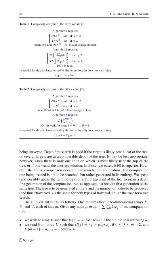
Table 1 Complexity analysis of the naive variant [2]

Algorithm 1 requires{ O(N m − m) if m ≥ 2

O(N 2 − m) if m = 1operations and O(N m − N ) bits of storage in total.

Algorithm 1 requires⎧⎨

⎩

O(⌈

Nm−mB

⌉)if m ≥ 2

O(⌈

N2−mB

⌉)if m = 1.

I/O’s in total.

Its spatial locality is characterised by the access locality function satisfying

L A(p) = p/N ′.

Table 2 Complexity analysis of the DFS variant [2]

Algorithm 5 requires{ O(N m − m) if m ≥ 2

O(N 2 − m) if m = 1operations and O(m) bits of storage in total.

Algorithm 5 requires

O(

N�(m)

N B−i

)

I/O’s in total, for some i = 0, . . . , B − 1.

Its spatial locality is characterised by the access locality function satisfying

L A(p) = logN ′ p.

being surveyed. Depth first search is good if the target is likely near a leaf of the tree,or several targets are at a comparable depth of the tree. It may be less appropriate,however, when there is only one solution which is most likely near the top of thetree, or if one wants the shortest solution. In those two cases, BFS is superior. How-ever, the above comparison does not carry on to our application. The computationtree being treated is not to be searched, but rather generated in its entirety. We speak(and possibly abuse the terminology) of a DFS traversal of the tree to mean a depthfirst generation of the computation tree, as opposed to a breadth first generation of thesame tree. The tree is to be generated entirely and the number of nodes to be produced(and thus “traversed”) is the same for both types of traversal, unlike the case for a treesearch.

The DFS variant is cast as follows. One requires three one-dimensional arrays K ,U , and V , each of size m. Given any node μ = v0 +∑�−1

j=0 k j e j of the computationtree,

• we write to array K such that K [ j] = k j for each k j in the �-tuple characterising μ,• we read from array U such that U [ j] = n j of edge e j , if 0 ≤ j ≤ m − 2, and

U [m − 1] = nm−1 − 1 otherwise,

123


• we read from array V such that V [ j] contains the coordinates in Z2 of the primitive

vector e j .

Using the same input as that of Algorithm 5, we proceed as follows:

Algorithm 5 [2]A. Main()Step 1: Initialise a global vector u ← v0, and a global boolean variable b← F AL SE.Call DFS-compute(0).Step 2: Return “Decomposable” if v0 is found in any of the leaves, and “Indecom-posable” otherwise.

B. DFS-compute( j)Step 1: K [ j] = 0.Step 2: While K [ j] ≤ U [ j] do:

2.1: If b = F AL SE and j = m − 1: Set b← T RU E and exit the loop.2.2: Compute u ← u + K [ j] · V [ j].2.3: If u ∈ P (or R) and j �= m − 1: Call DFS-compute( j + 1).2.4: u ← u − K [ j] · V [ j], K [ j] ← K [ j] + 1.

We now address the implicit assumptions observed in Ref. [2] and leading to thecosts in Theorem 2 if one were to reason in the RAM model. The first assumptionaffects testing for inclusion in P . Given an arbitrary point (a, b) in the plane, both thenaive and DFS-based algorithms assume that it takes constant time to answer the querywhether or not this point belongs to P . This may be possible, as shown in Ref. [1], bypre-processing on the given polygon, producing some form of “boundary” points: Forall vertices of P , let ymax and xmax denote the maximum vertex coordinates in the y andx directions respectively, and ymin and xmin denote the minimum vertex coordinates inthe y and x directions respectively. To perform the inclusion test almost for free in theRAM model, one would only need to store the boundary points, which requires a twodimensional integer array E of size 2× ymax, such that any arbitrary point (a, b) is in Pif and only if E0,b ≤ a ≤ E1,b. Let D = max (ymax, xmax). The entire pre-processingthen requires O(m2D) integer operations, as part of pre-computation.

A second assumption affects redundancies that may arise in vector computations.One obtains the costs in Theorem 2 if redundancies in vector computations are assumednot to carry from one iteration to the next, or more realistically, if redundancies areeliminated “cheaply”. One can achieve this for the naive variant using a flag matriximplemented as a two-dimensional array F . Manipulating the flags to eliminate redun-dancies costs O(tm) integer operations in total, if one were to assume that a memoryaccess costs as much as one arithmetic operation, and O(t) bits of auxiliary storage.Both costs can be embedded in the respective terms obtained in Theorem 2, if onewere to reason in the RAM model. For the DFS version, a flagging mechanism isdeveloped in Sect. 3 below, which also comes at no asymptotic loss in performance,if one were to ignore the effect of memory accesses.

The two assumptions however can no longer be simulated efficiently as one divergesfrom the purely computational RAM model towards the ideal cache model. Of par-ticular concern are the costs associated with accessing the boundary points array Eand flag matrix F . In Ref. [2], it is remarked that the three data-bound components of

123


Algorithm 1 (i.e. the vector computations, the inclusion test, and handling the redun-dancies) each has a completely independent memory access pattern. Only accessesto the arrays used to track the vector computations in both the naive and DFS-basedversions occur with some well defined patterns, whereas the access patterns associ-ated with array E for the inclusion test and matrix F for redundancy checking can becompletely irregular, with no means to measure this irregularity.

To work around the memory access costs associated with the inclusion test, a trade-off between computation and memory accesses is established in Ref. [2]. The trade-offallows more vector points to be carried from one iteration to the next, by resorting toa crude inclusion test that is less strict than the exact one: Given a convex polygonP , one can always embed the polygon in a smallest enclosing rectangle R. Given thecoordinates of the four vertices of this rectangle, one checks for the inclusion of anarbitrary point (a, b) in R by comparing each of a and b to the coordinates of thefour vertices. Despite that this may accept points that are in R but not in P , it stilldoes not affect correctness of the summand tracing algorithm [2]. Also, one can thengain by that the boundary points will no longer need to be stored and that the memoryaccesses to E can be eliminated altogether. Using the crude test would be a clear winif one can show that the increase in the number of vector operations and the associatedmemory accesses are not asymptotically more compelling than if one were to bear thememory accesses necessary to process the boundary points storage scheme. This maybe possible, for example, if the increase in the number of integral points as a result ofthe crude test is only a constant factor of the total number of integral points belongingto P . However, there are so far no means to control when such an increase in irrele-vant points will remain asymptotically affordable. At best, and crudely so, one hopesthat for very random polynomials, their Newton polygons will grow asymptoticallyalike to the smallest rectangle enclosing them, and we monitor this trade-of in ourexperiments.

In Ref. [2] it is proposed that redundancies in vector computations be tolerated,and a trade-off get measured between this increase in irrelevant vector computationsversus bearing the costs associated with the flagging mechanism. There could be somemeans by which one can predict redundancies before actually performing the redun-dant computations. We sketch a brief description in Sect. 3 but do not investigate itany further in the current paper.

Our empirical study is directed as follows: We first assess the DFS variant withregard to improvements affecting the pattern of vector computations only. Afterwards,we conduct experiments where we re-introduce the exact real inclusion test, and thenthe flag matrix for eliminating redundancies. The aim of those variations is to experi-mentally assess whether the gains obtained using the DFS variant remain significantdespite the memory intensive procedures for exact inclusion testing and resolvingredundancies. Indeed, our experiments certify this fact.

We conclude the background section by summarising the run time, space, and cachecomplexity analysis of both the naive and DFS variants as conducted in Ref. [2]. Theassumptions behind this analysis are that the crude inclusion test is employed, theredundancies are tolerated, and the number of vector points produced is boundedloosely from above, as a result of the worst-case scenario defined by that all vectorpoints are accepted by the inclusion test. We also assume that none of the initial

123


data structures fit in cache, for either variants. Let L A(n) denote the access localityfunction introduced in Ref. [5], which returns the maximal possible distance betweentwo elements of some list A and that are accessed within n contiguous operations.Let N ′ denote the minimum number of integral points on an edge of P . Recall thatD = max (ymax, xmax), and assume, without loss of generality, that D fits in a machineword. The resulting analysis is presented in the tables below:

3 Redundancies: handling and prediction

In this section we describe a flagging mechanism to resolve redundancies in the DFSvariant, and analyse the associated costs in the ideal cache model. We also sketch abrief description on how redundancies can be predicted.

Proposition 6 Redundancies arising in the DFS variant can be eliminated using aflag matrix and an index array at the following costs. Employing the flag matrix forhandling redundancies in the DFS variant incurs asymptotically as much time, space,and caching costs as in the naive variant. Employing the index array incurs asymp-totically as much time, space, and caching costs as in the DFS variant when it doesnot invoke any redundancy eliminating procedures.

Proof To eliminate redundancies in the DFS variant, we propose two arrays F and Ias follows. When initialised entries in F are set to−1 and entries of I are set to m− 1(we will justify later on both initialisation values). Throughout, F[x, y] = −1 impliesthat the lattice point (x, y) has not been produced in earlier vector computations. Else,F[x, y] = i ≥ 0 implies that the point (x, y) has already been produced using asequence of edge vectors {k j e j }, for j = 0, . . . , i , with some k j possibly zero. ArrayI embodies information as follows. Recall the global vector u defined in Algorithm5, and representing an arbitrary vector computation taking place at any one level j ofthe recursion tree (with starting level j = 0). The index i = I [ j] denotes an upperbound on the indices of vectors across which u may be further displaced, and abovewhich the associated vector displacements will certainly produce redundant vectors.

We illustrate the sequence of operations on each of F and I as follows. At the startof the algorithm initialise all entries of F to−1 and set I [0] = m− 1. Consider someiteration of the while loop within a recursive call DF S − compute( j), for j > 0,where the vector computation

u′ ← u + k j e j (1)

has to be performed. If I [ j] ≥ j – which is certainly the case at least initially, sinceI [0] is initialised to m − 1 > 0 – then this implies that the vector computation in (1)may not be redundant; else, the computation is definitely redundant, and we returnfrom level j of the tree. If the computation in (1) may not be redundant, it is performedand the resulting lattice point (x, y) is examined as follows:

1. If (x, y) is rejected by the inclusion test, then nothing is done, and we reset u′ toits original value u as in Step 2.4 of Algorithm 5, and proceed to the next iteration.

123


2. If (x, y) is accepted by the inclusion test, and F[x, y] = −1, this implies thatF[x, y] has not been produced during any earlier computation and thus is notredundant. One then sets F[x, y] = j , to denote that (x, y) has once been foundat level j of the recursion tree, and that the DFS traversal will displace u′ acrossall remaining possible paths down the tree, starting with level j + 1 downwards,for which we set I [ j + 1] = m − 1. It is understood, iteratively speaking, that allredundancies arising along those paths will be eliminated.

3. If (x, y) is accepted by the inclusion test, and F[x, y] �= −1, this implies that(x, y) has earlier been found at level i = F[x, y] of the recursion tree, and asa result of item 2 above, displaced across all remaining possible paths down thetree, starting with level i+1 downwards, with all redundancies arising along thosepaths eliminated. If we further have i ≤ j , this means that displacing (x, y) acrossany direction of e j (and downwards reaching the leaves) will be redundant, andso the computation in (1) is skipped. Otherwise, if i > j , the displacement in(1) and the ensuing ones taking place along all possible paths starting from levelj + 1 down to level i may not be redundant. In this case, one needs to updateF[x, y] = j , and restrict I [ j + 1] to be equal to i .

We now discuss the costs associated with the above mechanism. Assuming D fitsin a machine word, the flag matrix F is implemented as a two-dimensional integerarray of total size D2, which is the same size as it would require in the naive version(see Ref. [2], Section 2.4.2). Since each entry F[x, y] may only contain the index ofsome tail edge vector leading up to (x, y), and indices can only be in the range 0, . . .,m−1, the initialisation value−1 chosen for F is justified. Note that no computation isperformed on elements of F . Each vector computation requires O(1) memory acces-ses to an entry in F . In the worst-case analysis, each memory access to F requiresa separate I/O, which in total, is asymptotically equal to the total number of I/O’srequired by the naive algorithm employing the flagging technique (see Ref. [2], proofof Proposition 5).

Assuming m fits in a machine word, the index array I is used as follows. First,note that no computation is performed on elements of I . Initially, each vector pointshould be displaced along all possible paths down the DFS tree, reaching down to thelast level. This justifies why entries of I may be initialised to m − 1, and that arrayI must be an integer array of size m, which is the same size as arrays K , U , and V inAlgorithm 5. Also, note that we access both I [ j] and K [ j] a constant number of timesupon every call to DF S − compute( j). Thus, memory accesses to I mimic those toK both in their pattern as well as total number. By proof of Proposition 10 of Ref.[2], the total number and pattern of memory accesses to array K determine the cachecomplexity of Algorithm 5. This concludes the second part of the proof.

In order to predict redundancies, one needs to explore the relationship between thedifferent edge vectors. If two different vector expansions A and B can get to the samepoint p in the plane, this implies that there exists some linear dependence amongst asubset of the vectors appearing in one or both expansions, such that A − B = 0. Thenext question which arises is, when one is about to perform some vector expansion B,how can one predict a redundancy such that B = A, where A is a vector expansion

123


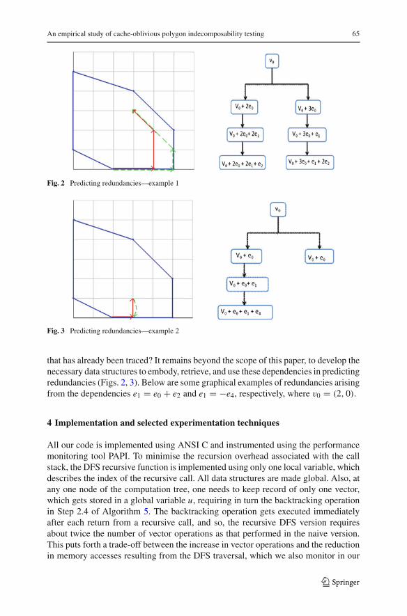
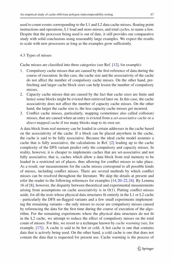
Fig. 2 Predicting redundancies—example 1

Fig. 3 Predicting redundancies—example 2

that has already been traced? It remains beyond the scope of this paper, to develop thenecessary data structures to embody, retrieve, and use these dependencies in predictingredundancies (Figs. 2, 3). Below are some graphical examples of redundancies arisingfrom the dependencies e1 = e0 + e2 and e1 = −e4, respectively, where v0 = (2, 0).

4 Implementation and selected experimentation techniques

All our code is implemented using ANSI C and instrumented using the performancemonitoring tool PAPI. To minimise the recursion overhead associated with the callstack, the DFS recursive function is implemented using only one local variable, whichdescribes the index of the recursive call. All data structures are made global. Also, atany one node of the computation tree, one needs to keep record of only one vector,which gets stored in a global variable u, requiring in turn the backtracking operationin Step 2.4 of Algorithm 5. The backtracking operation gets executed immediatelyafter each return from a recursive call, and so, the recursive DFS version requiresabout twice the number of vector operations as that performed in the naive version.This puts forth a trade-off between the increase in vector operations and the reductionin memory accesses resulting from the DFS traversal, which we also monitor in our

123


performance analysis. The experiments performed are conducted using eight variants.Firstly, one needs to measure the naive against the DFS variant. For each of those,a variant may employ a flagging mechanism (in which case we label it as “flagged”),or may not (so that it becomes “un-flagged”). A flagged (or un-flagged) variant mayemploy the crude inclusion test (in which case we label it as “crude”), or the realinclusion test (so that it becomes “real”).

We borrow experimental definitions from Ref. [18] to describe our objects of anal-ysis. In our experiments, we generate resource measurements for temporal locality,defined as the miss rate of (L1 and L2) caches over a window of instructions. Spatiallocality (measured as the average fraction of a cache line over a window of instruc-tions) has been proven to be optimal for the DFS variant, and so we do not addressthis in our measurements.

4.1 Instrumentation tool: PAPI

PAPI stands for Performance API or Performance Application Programming Interface.PAPI is used to access hardware performance counters, which are available on majorprocessors today in order to count events that occur during the execution of a program.Hardware performance counters count the occurrences of certain signals associatedwith a processor’s function. PAPI acknowledges an important type of set events calledthe preset events, usually found in CPUs that have performance counters and accessto the memory hierarchy. The PAPI preset event library includes approximately 100preset events such as cache and TLB misses, hits, reads, writes, accesses, etc., alongwith events that count the number of cycles, FLOPs, instructions, etc. Not all eventsare available on all platforms. Hence, to determine which events are available on aspecific platform, an event query function can be called. In order to monitor a certainevent or a set of events during the execution of a specific run, an event set is createdand the desired event(s) are added to it. PAPI event counters are grouped in compatiblegroups and the PAPI event chooser utility can be used to determine the compatibilitybetween the chosen events counters. In other words, one can only monitor events thatare compatible in a single run. The compatible events are specific to each machine. Forthe machine we use in our experiments, L2 data cache misses can only be monitoredwith either L2 instruction cache misses or L2 total cache misses. On the other hand,L1 data cache misses can be monitored along with any one of a list of 35 events.A few examples of those are L1 instruction cache misses, total cycles, L1 load misses,L1 data cache accesses, along with many others.

4.2 Hardware

We conduct our experiments on an Intel Pentium III processor, with a single nodeCPU, and a speed of 797 MHz. The machine has an L1 data cache of total size equalto 16 KB, consisting of 512 cache lines, each of size 32 Bytes. The machine has anL2 data cache of total size equal to 256 KB (which is shared by instructions and data),consisting of 8192 cache lines, each of size 32 Bytes. The size of the main memory is384 MB. There are two hardware counters available on this machine. The counters are

123


used to count events corresponding to the L1 and L2 data cache misses, floating pointinstructions and operations, L1 load and store misses, and total cycles, to name a few.Despite that the processor being used is out of date, it still provides our comparativestudy with solid conclusions using reasonably large examples. We expect the resultsto scale with new processors as long as the examples grow sufficiently.

4.3 Types of misses

Cache misses are classified into three categories (see Ref. [12], for example):

1. Compulsory cache misses that are caused by the first reference of data during thecourse of execution. In this case, the cache size and the associativity of the cachedo not affect the number of compulsory cache misses. On the other hand, pre-fetching and larger cache block sizes can help lessen the number of compulsorymisses.

2. Capacity cache misses that are caused by the fact that cache sizes are finite andhence some blocks might be evicted then retrieved later on. In this case, the cacheassociativity does not affect the number of capacity cache misses. On the otherhand, the larger the cache size is, the less capacity cache misses get incurred.

3. Conflict cache misses, particularly, mapping (sometimes also called collision)misses, that are caused when an entry is evicted from a set-associative cache or adirect-mapped cache if too many blocks map to its own set.

A data block from real memory can be loaded in certain addresses in the cache basedon the associativity of the cache. If a block can be placed anywhere in the cache,the cache is said to be fully associative. Because the ideal cache model assumes acache that is fully associative, the calculations in Ref. [2] leading up to the cachecomplexity of the DFS variant predict only the compulsory and capacity misses. Inreality, however, it is cheaper to implements caches that are set-associative and notfully associative; that is, caches which allow a data block from real memory to beloaded in a restricted set of places, thus allowing for conflict misses to take place.As a result, our measurements for the cache misses correspond to all possible kindsof misses, including conflict misses. There are several methods by which conflictmisses can be resolved throughout the literature. We skip the details at present andrefer the reader to the following references for examples [14,20–22,24]. By Lemma16 of [8], however, the disparity between theoretical and experimental measurementsarising from assumptions on cache associativity is in O(1). Putting conflict missesaside, for all the tests whose physical data structures fit entirely in the L1 or L2 cache- particularly the DFS un-flagged variants and a few small experiments implement-ing the remaining variants—the only misses to occur are compulsory misses causedby referencing the data for the first time during the course of execution of the algo-rithm. For the remaining experiments where the physical data structures do not fitin the L2 cache, we attempt to reduce the effect of compulsory misses on the totalcount of misses. For this, we resort to a technique known by cache warming (see, forexample, [17]). A cache is said to be hot or cold. A hot cache is one that containsdata that is actively being used. On the other hand, a cold cache is one that does notcontain the data that is requested for present use. Cache warming is the process of

123


turning a cold cache into a hot one, and is achieved by pre-loading the data neededinto the cache before it is actually referenced, which improves the performance ofthe application by minimising the effect of compulsory misses, and hence achievingconsistent and reliable results when comparing amongst several experiments. Alter-natively, one could run any one code twice and subtract the cache misses countsresulting from both runs, thus deducting the number of compulsory misses from thetotal count.

4.4 Windows of instructions

For all of the flagged variants, we measure the cache performance over the entireexecution window, since the tests for such variants terminate in a reasonable amountof time. For the un-flagged variants, we resort to the windowing technique describedin Ref. [18]. Because redundancies are preserved in the un-flagged variants, the run-ning time and space requirements become exponential in N (see Tables 1, 2). Tocircumvent this, we limit ourselves to measuring the cache performance over a win-dow of instructions required to compute the maximum number of vector points thatcan fit in memory. Based on the available machine, and bearing that one would needat most four integer arrays to process both unflagged variants, it turns out we canprocess roughly up to 16 × 106 vector operations. More details on this appear inSect. 5.3.

5 The input polygons

We are interested in polygons which are effectively Newton polygons of bivariatepolynomials. The Newton polygon of a bivariate polynomial with t non-zero termswill have at most t edges. As before, recall that ymax and xmax denote the maximumvertex coordinates in the y and x directions respectively, and ymin and xmin denotethe minimum vertex coordinates in the y and x directions respectively. A non-trivialinput to the absolute irreducibility testing algorithm will be a non-constant polynomialwhich is known not to be reducible, and which is not divisible by any monomial ofthe form xe1 ye2 , for some integers e1, e2 ≥ 0. Given a bivariate polynomial that is notdefinitely known to be reducible, its Newton polygon must contain at least one vertexon the x-axis and one vertex on the y-axis—see Ref. [1], Lemma 7. Therefore, we canassume that ymin = xmin = 0. Recall that D = max (ymax, xmax). Let d be the totaldegree of f . Then the degree of f in x or y will be at least d/2 and at most d, so that2/d ≤ D ≤ d.

Our choice of input is affected by the kind of memory performance we wish to solicitand the various input parameters which affect this performance. Primarily, we aim forinput instances where the associated data structures do not fit in the L2 cache. In theremainder of this section, we let d denote the total degree of the input polynomial fand t the total number of its non-zero terms. We also let D denote the maximum dimen-sion of the smallest rectangle R enclosing Newt( f ), m the total number of edges ofNewt( f ), Z the total number of lattice points belonging to Newt( f ), and N and N ′ themaximum and minimum number of integral points along any edge of Newt( f ). For all

123


flagged variants as well as the variants employing the naive algorithm, manipulatingthe maximum dimension D causes the flag matrix and/or the vector arrays {Ai }0≤i<m

to grow in size. The other remaining parameters whose effect must be gauged are m,as well as the edge lengths {ni }, which in turn are bounded by N and N ′ from aboveand below, respectively. Recall also that m ≤ t , and that N ′ and N are in O(D).

5.1 Manipulating the number of edges m

One can easily construct random polynomials whose Newton polygons have a num-ber of edges that is determined a priori, provided no control is sought over the edgelengths {ni }. We determine a range for the maximum dimension D to be chosen from500, 1,000, 1,500, 2,000, and 2,500, and we seek five sets of convex polygons whereeach set corresponds to a given dimension in this list. Each of these five sets consists ofthree random convex polygons to be constructed using 250, 1,000, and 5,000 randompoints in the plane, respectively. Equivalently, one can say that such polygons will cor-respond to three random polynomials having 250, 1,000, and 5,000 non-zero terms,respectively. In addition, we seek the convex polygons in such a way that allows us tomonitor the effect of increasing values of m on the overall performance, and so, werequire that a polygon chosen at random have a pre-determined number of edges. Forthis, we first try generating random polynomials of degree at most D using a randomnumber generator, and with a pre-determined number of terms, after which the asso-ciated Newton polygons are constructed. In most of the cases, this results in Newtonpolygons with very small edges. For example, setting t = 75,000 for D = 2,500results in a Newton polygon with at most 27 edges. To gain better control over thechoice of m, we try instead a trigonometric approach as follows ([23], p. 44). We firstdetermine an upper bound on m. Call this upper bound c. We then construct a circlecentered at (D/2,D/2) and with diameter equal to D. Let r denote the radius of thecircle. One then produces c points on the boundary of the circle defined as follows:

pi = xi + yi , where xi = r + r · cos(2iπ/c), yi = r + r · sin(2iπ/c),

and i = 0, . . . , c − 1. This produces c points on the circumference of the circle,which, if connected, determine all the vertices of a convex polygon. However, notall of the points are guaranteed to be integral points, because of the real summandsarising from the trigonometric functions appearing in xi and yi . A slight modification(say by taking the floor or ceiling of the trigonometric return values) produces a setof c′ ≤ c integral points that are not necessarily on the boundary, but that are theclosest integral points to the original real counter-parts. One then takes the convexhull of such c′ integral points. Note that this method ensures that at least one vertexof the resulting convex polygon lies on the x-axis and at least another vertex lies onthe y-axis. Heuristically speaking, the method tends to produce convex polygons withgreater number of edges than simply randomising a certain polynomial then taking itsNewton polygon. The resulting polygons also have random lower and upper boundsN ′ and N on the number of points along any edge. After the polygons are obtained, weassociate with each polygon a bivariate polynomial whose non-zero terms correspond

123


to the original c points randomly chosen at the beginning. A table summarising theproperties of our 15 input polygons and associated polynomials appears in Ref. [3].

Remark 7 It appears that for all such random input polygons, the actual size of thepolygon is within at least 80% of the size of the smallest enclosing rectangle. Thisimplies that for all of our runs which employ the crude rather than the real inclusiontest, a reliable comparison can be derived regarding the performance of both the naiveand DFS variants.

5.2 Manipulating the edge lengths {ni }

We now aim for a set of polygons by fixing m and varying the edge lengths {ni }. Wedivide the pool of input into test sets representing polygons having maximum dimen-sion D chosen from 100, 250, 750, 1,000, 1,500, 2,000, and 2,500 respectively. Theupper limit on D is constrained by the greatest upper bound on the memory require-ments of all variants, which is in O(D)2. Finally, all the chosen polygons have N ′ = 1or 2, whilst the upper bound N is manipulated. The edge lengths {ni } are chosen tobe in the range N ′ to N , with the first edge having the largest length, the second edgehaving the next largest, and so on and so forth. For a given tuple of lengths, this permu-tation of the edge lengths maximises the cache complexity of the DFS variant (checkproof of Proposition 10 of [2]), and so solicits worst-case performance for the DFSvariant, but no particular effect on the naive variant. We now sketch the mechanismby which such polygons are constructed. Given m, D, N ′, and N , each polygon mustconsist of m vertices and associated polygonal lines whose smallest enclosing rectan-gle has a maximum dimension equal to D. We construct the vertices and polygonallines as follows. Here, we take m to be the total number of polygonal lines comprisingthe polygon, and refer to polygonal lines as edge vectors. The set of vertices can beobtained in four batches according to the following restrictions. Each batch is to con-sist of an arbitrary number of vertices, such that the total number of vertices acrossall batches is equal to m. All vertices should respect the boundaries of the rectangleR, so that their x and y-coordinates are bounded from below by 0 and from aboveby D. The vertices are chosen to ensure that the number ni of integral points on eachedge vector Ei satisfies N ′ ≤ ni ≤ N and ni ≥ ni+1. Since the last vertex, say v�,in any of the four batches has to fall on one of the boundary edges of R, this mightforce us to choose n� completely randomly between N and N ′, regardless whether itsatisfies n� ≤ n�−1. Eventually, the first batch consists of vertices whose x-coordi-nates position them between the lowest and rightmost points. Continuing analogously,we aim for the second batch to consist of vertices whose y-coordinates position thembetween the rightmost and highest points, the third batch to consist of vertices whosex-coordinates position them between the highest and leftmost points, and the fourthbatch to consist of vertices whose y-coordinates position them between the leftmostand lowest points. Finally, edge vectors are constructed such that no two consecutiveedge vectors are parallel. We observe that this procedure does not necessarily result inconvex polygons. In contrast to the pool of convex polygons obtained above, whichcan be used to test both the real and crude variants, the current pool can only beguaranteed to work for testing the crude variants. Our justification for still using it

123


is that, for all crude versions, and in the worst-case analysis, the run time and cachecomplexity of both the naive and DFS-based versions can be expressed entirely as afunction of the edge lengths as well as the number of edges, and all the vector pointsfall in an enclosing rectangle rather than strictly within the actual polygon. Convexityof the input polygon is thus essential only for correctness of the summand tracing algo-rithm and bears no effect on termination, run time or cache complexity. As such, wecompromise on the convexity of the sought polygons by creating “fake” inputs whichsimply consist of connected polygonal lines not necessarily closing up on a convexpolygon and thus which cannot be associated with bivariate polynomials. With this,the crude variants end up being tested from the viewpoint of being “general solvers”,and the comparisons regarding performance analysis hold irrespective of whether ornot the input polygons are “valid” or “real”. We refer the reader to Ref. [3] for a tablesummarising the properties of the resulting polygons, which, by abuse of notation, weshall call them concave.

5.3 Memory requirements

Given a bivariate polynomial f , recall that D denotes the maximum dimension ofthe smallest rectangle R enclosing Newt( f ), m denotes the total number of edgesof Newt( f ), and N the maximum number of integral points belonging to an edge ofNewt( f ). For the naive variants, we let A denote the size of the largest array Ai ofvectors. Assume that D fits in a machine word (so that N and all vector coordinatesalso do). Assume also that m fits in a machine word. All arrays are thus integer arrays,where one integer is assumed to require four Bytes.

The parameter A affects only the naive variants, but bearing that the unflaggednaive variant requires that we limit the number of vector operations to the maximumpossible, A may reach up to roughly 16× 106, according to the machine on which weperform our experiments. The parameter m affects all variants. It determines the sizeof the arrays containing the coordinates of the vertices of Newt( f ) as well as its edgevectors. It also determines the size of the index array I used to enforce the flaggingstrategy in the DFS variant. The parameter D affects the variants employing the realinclusion test only and determines the size of array E describing the boundaries of thepolygon. The parameter D2 affects all flagged variants and determines the size of theflag matrix F . In effect, we also have A = O(D2) for the flagged naive variants, sinceby eliminating redundancies one cannot trace more than D2 lattice points belongingto Newt( f ).

We now determine which of the input instances from both the convex and con-cave pools cause the associated data structures to fit, or else, exceed the L1 and L2caches. We do this by obtaining a rough estimate in Megabytes required for such datastructures, depending on the variant being employed. We illustrate with an examplewhich can be mimicked across all other inputs and variants. Consider for instance, theun-flagged naive variant employing the real inclusion test, and examine the input fromthe convex pool with D = 500, t = 250 and m = 94. The associated data structureswill require four vector arrays of size A, the E array of size 2D, and six arrays of sizem for manipulating the vectors, all of which require roughly about

123


4(

4A+ 2D + 6m = 4× 16× 106 + 2× 500+ 6× 94)× 10−6 Bytes

= 256.006256 MB.

Similar calculations follow for the remaining two polygons having D = 500. We takethe maximum of those three values, which turns out to be 256.007240 MB, and asso-ciate it with D = 500. Again, we perform similar calculations taken over all possibleinputs and all possible variants. Recall that the size of the L1 data cache of the availablemachine is 16 KB and the size of the L2 cache, which is shared by instructions anddata, is 256 KB. The resulting terms in MegaBytes help us derive conclusions as towhich data structures fit in which caches, which in turn helps us assess the types ofmisses we report on in our experiments, and how this affects the comparison amongstthe various variants being tested.

6 Experimental results and performance analysis

In this section we present a summary of our experimental results and performanceanalysis, and refer the reader to Ref. [3] for detailed tables of measurements as wellas extensive analysis of the results.

Recall that in the case of the un-flagged variants, we resort to the windowing tech-nique described above, in which we limit both the naive and DFS unflagged variantsto producing only 16× 106 vector points. For the flagged variants, both the DFS andnaive algorithms are traced until final execution.

6.1 Convex: unflagged crude variants

We assess the results of this section using the convex pool of input. Note that all inputpolygons for this set of experiments do not cause the data structures associated withthe DFS unflagged variant to exceed the L2 cache. In such cases, all misses reportedfor the DFS variant are either compulsory or conflict, but not capacity misses.

We note that the total number of FLOPS taken by the DFS variant is always greaterthan the total number of FLOPS required by the naive algorithm, as indeed explainedin our discussion on backtracking above. Still, the percentages of improvement in thetotal number of L1 and L2 misses are spectacular—reaching about 99%. The percent-ages of improvement in the total number of cycles are realistically smaller, due to theoverhead of computation, but still around a satisfactory average of 30%, and reach-ing up to 60%. The percentages of improvement in cycles decreases with increasingm, since, for a fixed number of vector operations, the memory performance of theDFS variant is sensitive to the increase in this parameter, whilst the naive algorithmis not.

6.2 Convex: flagged crude variants

We assess the results of this section using the convex pool of input. We still noticea significant improvement in the L1 and L2 misses. However, the fact that we are

123


experiencing capacity and not only compulsory misses makes the effect of the smallsize of the L1 cache more significant. Particularly, the percentages of improvementobserved for the L1 misses are noticeably less than what is observed for the corre-sponding term in the unflagged tests. The percentages of improvement in the totalnumber of execution cycles are significantly lower than what is observed for the L1and L2 misses, despite reaching in numerous cases a relatively satisfactory 15–35%.Still, the fact that such percentages remain visible in the range 15–48% shows thatdespite the overheads of the flag matrix, the DFS variant continues to outperform thenaive algorithm. Finally, despite that the total number of FLOPS taken by the DFSvariant is larger, its overall performance in cycles is better, which supports the trade-off between extra computations and decreased memory accesses associated with theflagged DFS variant.

6.3 Convex: unflagged real variants

We assess the results of this section using the convex pool of input. The percentages ofimprovement in the total number of L1 and L2 cache misses are spectacular, enhancedby the fact that whilst the misses incurred by the DFS variant do not include capacitymisses, the naive algorithm does. The percentages of improvement in the total num-ber of cycles are realistically smaller, due to the overhead of computation, but stillaround a high average of 49%, and ranging between 40 and 55%. The satisfactorypercentages of improvement in cycles can be interpreted to say that memory accessesare a bottleneck for the naive unflagged variant, despite that the effects of handlingredundancies have been filtered out. We finally note that, unlike for the variants incor-porating the crude test, the percentages of improvement in cycles do not necessarilyincrease with increasing m, since both the DFS and the naive variants are now sensitiveto the increase in D, which in turn can trigger unpredictable memory access patternsassociated with the boundary array E .

6.4 Convex: flagged real variants

We assess the results of this section using the convex pool of input. For both flaggedvariants, the cache misses reported include capacity misses in addition to compulsoryand conflict misses, as the flag matrix introduced causes the initial data structuresto exceed the L2 cache. We still notice a significant improvement in the L1 and L2misses. However, the fact that we are experiencing capacity and not only compulsorymisses makes the effect of the small size of the L1 cache more significant. Particularly,the percentages of improvement observed for the L1 misses are noticeably less thanwhat is observed for the corresponding terms in the unflagged tests and it is around anaverage of 25%, and range between 2 and 71%. Still, the percentages of improvementin the L2 misses are high with an average around 77%, and range between 33 and98%. The percentages of improvement in the total number of execution cycles aresignificantly lower than what is observed for the L1 and L2 misses, despite reach-ing in numerous cases a relatively satisfactory average of 21%, with the percentagesranging between 2 and 82%. Still, the fact that such percentages remain visible in the

123


range 2–82% shows that despite the overheads associated with the flag matrix and theboundary points array E , the DFS variant continues to outperform the naive algorithm.

Despite that the total number of FLOPS taken by the DFS variant is larger, itsoverall performance in cycles is better, which supports the trade-off between extracomputations imposed by the crude variant—causing additional memory accessesto the associated data structures—and decreased memory accesses associated withaccessing the boundary points array E .

6.5 Flagged DFS variants: real versus crude

We compare the results of the flagged DFS variants employing the real versus the crudeinclusion tests using the convex pool of input. The percentages of improvement in thetotal number of L2 misses and in the total number of cycles imply that in all test casesthe real variant performs better than the crude variant. The satisfactory percentages ofimprovement in cycles of the real variant can be interpreted to say that memory acces-ses of the boundary points array E are not a bottleneck, while the extra computationsperformed by the crude variant, which in turn incur their own memory accesses, aremore compelling. Put differently, we conclude that incorporating the real inclusiontest does not affect adversely the improvements brought about by the DFS variant.

6.6 Concave: unflagged crude variants

We assess the results of this section using the concave pool of input. The aim of suchexperiments is to assess the effect of variations on N , for a given fixed m. The per-centages of improvement in the total number of L1 and L2 misses are spectacular,enhanced by the fact that whilst the misses incurred by the DFS variant do not includecapacity misses, the naive algorithm does. The percentages of improvement in thetotal number of cycles are realistically smaller, due to the overhead of computation,but still around a satisfactory average of 48%, and ranging between 42% and reachingup to 51%. The satisfactory percentages of improvement in cycles can be interpretedto say that memory accesses are a bottleneck for the naive unflagged variant, despitethat the effects of handling redundancies have been filtered out. We finally note thatthe percentages of improvement in cycles stagnate with increasing N . However, thosepercentages of improvement are more sensitive to m and D.

We now compare the L1 misses, L2 misses and total cycles percentages of improve-ment to their analogous (convex) ones in Sect. 6.1. We notice that the percentagesattributed to the concave tests for the same D are higher than those attributed to theconvex tests. This is due to the fact that the naive performance decreases as N increases.In all cases, the naive variant requires about twice the number of cycles required bythe DFS variant in order to perform any of the tests.

6.7 Concave: flagged crude variants

We assess the results of this section using the concave pool of input. We still noticea significant improvement in the L1 and L2 misses. However, the fact that we are

123


experiencing capacity and not only compulsory misses makes the effect of the smallsize of the L1 cache more significant. Particularly, the percentages of improvementobserved for the L1 misses are around an average of 58%, and range between 12 and98%, whilst the percentages of improvement in the L2 misses are around an averagearound 66%, and range between 7 and 99%. The percentages of improvement in thetotal number of execution cycles are significantly lower than what is observed for theL1 and L2 misses, but still reaching in numerous cases a relatively satisfactory averageof 40%, with the percentages ranging between 11 and 65%. Still, the fact that suchpercentages remain visible in the range 11–65% shows that despite the overhead ofthe flag matrix, the DFS variant is still superior.

The remainder of this section is dedicated to investigating the effect of the differentparameters on the percentages of improvement. We begin by observing the effect ofincreasing D and N on the L1 and the L2 percentages of improvement. The increasein D causes a decrease in L1 and L2 cache misses percentages of improvement. Thiscan be justified by the fact that the size of the flag matrix grows with D, such thatmemory accesses to this flag matrix may suffer from extremely low locality for boththe naive and the DFS variants. As the value of N increases, we also note a decrease inthe percentages of improvement in L1 and L2 misses. With increasing N , more vectoroperations are being performed, where each vector operation might trigger a separateI/O, as discussed earlier, bringing the number of cache misses incurred by the DFSvariant asymptotically closer to that incurred by the naive variant.

We now observe the effect of increasing D and N , both resulting in an increasein the percentages of improvement in the total cycles, despite that the DFS variant’scache performance deteriorates as the parameters D and N increase. We explain this asfollows. As D and N increase, the number of vector computations performed increaseas well, and so do the total number of FLOPS taken by the DFS variant. But the DFSvariant seems to perform those computations more efficiently than the naive variant,which supports the trade-off between the extra computations imposed by backtracking.

Finally, we observe that the rates of increase in the L1 misses, the L2 misses, andthe total cycles are higher for the naive variant than they are for the DFS variant.A similar observation holds when only m is increased.

6.8 Benchmarks: MAGMA

Finally, we benchmark the DFS variant against the powerful computer algebra sys-tem MAGMA [6]. The benchmarking experiments were conducted on an Intel Xeonmachine, with a 2GB main memory. MAGMA cannot test absolute irreducibility ofbivariate polynomials; instead, it can only test for irreducibility of bivariate polyno-mials whose coefficients come from some given ring. The pool of input to this setof experiments consists of four sets of significantly sparse, random bivariate polyno-mials, each chosen with a given number of terms, and derived from random Newtonpolygons having a maximum dimension D = 3,000, 4,000, 5,000, and 6,000 respec-tively. For those polynomials fed into the polytope method, we run the MAGMA codeto test irreducibility of the corresponding polynomials modulo primes ranging from2 until 37. We first examine the behaviour of the DFS variant versus MAGMA by

123


fixing D as well as the prime p denoting the order of the ground field. The remainingparameters are then allowed to vary. We observe that the DFS variant outperformsMAGMA by at least 88% to at most 100% across all of the experiments.

Next, we re-interpret the results by fixing the degree as well as the number of termsof the input polynomial. The prime order of the ground field is allowed to vary from2 until 37. We notice that the DFS variant remains insensitive to the increase in theunderlying prime, whilst MAGMA’s execution time increases, sometimes substan-tially, with increasing primes. Moreover, we note the two examples for D = 6,000and t = 100, with p = 19 and p = 37 respectively. In those tests, MAGMA fails torun due to insufficient memory, while the DFS variant executes successfully in about0.4 s. Both versions, however, experience an increase in run time as a result of fixingthe number of terms as well as the underlying prime, but varying the total degree of theinput polynomial. Finally, we consider very large degree polynomials, whose Newtonpolygons satisfy D = 7,000 and 10,000 respectively. After more than 4 h, MAMGAfails to terminate whilst processing any such large polynomial, no matter what groundfield is chosen. The DFS variant successfully tests all of these in a significantly lessertime. Finally, the DFS variant is used to test a polynomial of total degree 19640, inabout 2.9 s. We attribute this disparity to the following. Recall that MAGMA doesnot test for absolute irreducibility but rather for the weaker irreducibility propertyover a given ring (in our examples, a finite field). The algorithms used in MAGMA toachieve this over finite fields of prime order (taken, say, from the first and fourth refer-ences appearing in http://www.magma.maths.usyd.edu.au/magma/htmlhelp/text308.htm) are dense. That is, their run-time and space complexity are insensitive to thenumber of non-zero terms of the input polynomial. Those algorithms also grow withthe prime order of the underlying field. In contrast, the Newton polytope method fortesting irreducibility is sensitive to the number of vertices of the Newton polygon,which in turn is upper-bounded by the number of non-zero terms. It also does notget affected by the growth of the prime order of the ground field. This makes thepolytope method for testing irreducibility significantly faster for sufficiently sparsepolynomials, like the ones we have tested, or for polynomials over fields with largeprime order.

7 Conclusion

In this paper we present a comprehensive empirical study of a cache oblivious algo-rithm for testing absolute irreducibility of bivariate polynomials. Our contributionscan be summarised as follows. The proposed work is complementary to Ref. [2], inthat we address the practical usefulness of the cache-oblivious DFS-based variant, andcarry thorough experimentation to compare it against the naive version. The fact thatthe space, run-time, and caching costs associated with the DFS variant all depend onmore than one parameter require that we tailor our input and evaluate the resultingperformance in a way that manipulates those several parameters. In many times ourresults show spectacular improvements in the rates of cache misses, and reasonablyhigh improvements in the overall run-time. The benchmarks against MAGMA areequally in favour of the DFS variant, which either works faster or else is capable of

123

http://www.magma.maths.usyd.edu.au/magma/htmlhelp/text308.htm

http://www.magma.maths.usyd.edu.au/magma/htmlhelp/text308.htm


processing significantly larger degree polynomials that MAGMA cannot. Our work isalso essential for testing the feasibility of the trade-offs proposed in Ref. [2], specifi-cally as they affect testing for inclusion and eliminating redundancies. The concludingremark is that the DFS variant performs generally significantly better than the naivevariant even when one imposes data intensive procedures for performing those twotasks.

Acknowledgments The authors thank the Centre for Advanced Mathematical Sciences at the AmericanUniversity of Beirut for allowing the use of their facilities to perform the reported experiments. The firstauthor also thanks the Lebanese National Council for Scientific Research for supporting phases of thiswork.

References

1. Abu Salem FK (2008) An efficient sparse adaptation of the polytope method over Fp and a record-highbinary bivariate factorisation. J Symb Comput 43(5):311–341

2. Abu Salem FK. Cache-oblivious polygon indecomposability testing. Pre-print. http://www.cs.aub.edu.lb/fa21/Papers/COIrredTheory.pdf

3. Abu Salem FK, Soudah RN, Extended report on empirical, cache-oblivious polygon indecomposabilitytesting. Technical Report. http://dr.aub.edu.lb/file.php/2/moddata/data/3/24/1509/Paper.pdf

4. Aggarwal A, Vitter JS (1988) The input/output complexity of sorting and related problems. CommunACM 31(9):1116–1127

5. Bader M, Zenger C (2006) Cache oblivious matrix multiplication using an element ordering based onthe Peano curve. In: Proc. PPAM 2006, pp 1042–1049

6. Bosma W, Cannon J, Playoust C (1997) The Magma algebra system I. the user language. J SymbComput 24(3-4):235–265

7. Duval D (1991) Absolute factorization of polynomials: a geometric approach. SIAM J Comput 20:1–218. Frigo M, Leiserson CE, Prokop H, Ramachandran S (1999) Cache-oblivious algorithms. In: Proceed-

ings of the 40th annual symposium on foundations of computer science, pp 285–297, 19999. Gao S (2001) Absolute irreducibility of polynomials via Newton polytopes. J Algebra 237:501–520

10. Gao S (2003) Factoring multivariate polynomials via partial differential equations. Math Comput72:801–822

11. Gao S, Lauder AGB (2001) Decomposition of polytopes and polynomials. Discrete Comput Geom26:89–104

12. Hill MD, Smith AJ (1989) Evaluating associativity in CPU caches. IEEE Trans Comput 38(12):1612–1630

13. Kaltofen E (1985) Polynomial-time reductions from multivariate to bi- and univariate integral poly-nomial factorisation. SIAM J Sci Comput 14:469–489

14. Kharbutli M, Solihin Y, Lee J (2005) Eliminating conflict misses using prime number-based cacheindexing. IEEE Trans Comput 54(5):573–586

15. Lenstra AK (1985) Factoring multivariate polynomials over finite fields. J Comput Syst Sci 30(2):235–248

16. Lenstra AK (1987) Factoring multivariate polynomials over algebraic number fields. SIAM J Sci Com-put 16(3):591–598

17. Luo Y, John LK, Eeckhout L (2004) Self-monitored adaptive cache warm-up for microprocessorsimulation. In: 16th symposium on computer architecture and high performance computing, 2004.SBAC-PAD 2004, pp 10–17

18. Murphy RC, Berry J, McLendon W, Hendrickson B, Gregor D, Lumsdaine A (2006) DFS: a simpleto write yet difficult to execute benchmark. In: Proceedings of the IEEE international symposium onworkload characterizations IISWC06 2006, pp 175–177

19. Ostrowski AM (1921) Uber die bedeutung der theorie der konvexen polyeder fur die formale algebra.Jahresberichte Deutsche Math Verein 30:98–99

20. Patel K, Benini L, Marcii E, Poncino M (2006) Reducing conflict misses by application-specific re-configurable indexing. IEEE Trans Comput-Aid Des Integr Circuits Syst 25(12):2626–2637

123

http://www.cs.aub.edu.lb/fa21/Papers/COIrredTheory.pdf

http://www.cs.aub.edu.lb/fa21/Papers/COIrredTheory.pdf

http://dr.aub.edu.lb/file.php/2/moddata/data/3/24/1509/Paper.pdf


21. Rivera G, Tseng C-W (1998) Eliminating conflict misses for high performance architectures. In: pro-ceedings of the 12th international conference on supercomputing, pp 353–360

22. Rivera G, Tseng C-W (1998) Data transformations for eliminating conflict misses. ACM SIGPLANNotices 33(5):38–49

23. Thomas GB, Finney RL, Maurice WD, Giordano FR (2003) Thomas’ Calculus. Addison-Wesley,Reading

24. Zhang C (2006) Balanced instruction cache: reducing conflict misses of direct-mapped caches throughbalanced subarray accesses. IEEE Comput Architect Lett 5(1):2–5

25. von zur Gathen J, Kaltofen E (1985) Factorization of multivariate polynomials over finite fields. ApplMath Comput 45(171):251–261

123

an empirical study of cache-oblivious polygon indecomposability testing

Documents