An Environmental Mapping System for Airborne Particulate Matter

Monitoring in Urban Areas

DANIEL DUNEA

EMIL LUNGU

ALIN POHOATA

Valahia University of Targoviste

Blvd. Unirii, no.18-24, Targoviste, 130084,

ROMANIA

dunea@valahia.ro http://www.rokidair.ro/en

Abstract: - The paper presents the functional characteristics of an environmental mapping system (EMS) for

presenting air quality data according to their geographic location and spatial topologies. The basic components

of a web-based GIS system were presented namely, the map server, and the application interface for displaying

the thematic layers in a web page. It exemplifies the developing of a map file used by the mapping server and

an .html file for the web page, which displays a thematic map that interpolates at spatial scale the measurements

of the airborne particulate matter in an urban agglomeration.

Key-Words: - PM2.5, air pollution, web-based GIS, geospatial data, kriging interpolation, thematic layers.

1 Introduction The researches in the fields of air quality and

related epidemiology take into account the analysis

of several factors for the development of

correlations and the deduction of knowledge that

can be used for early forecasts required to establish

protection measures for population [1]. The study of

these factors involves the collection and

investigation of large amounts of data to obtain

conclusive results (close to the real situations) [2-4].

Therefore, it is important to optimally organize the

data for processing and that the data analysis will be

efficient in terms of time required to obtain a valid

response to the environmental problem [5].

The presentation of the air quality data to the

interested public must be made to non-specialists in

an accessible form. The public is generally

interested in graphical representations and synthetic

environmental indices with quick impact for

understanding complex phenomena based on the

data that substantiated the drawn conclusions [6].

The issue of studying the fine particulate matter

(PM2.5) is very complex and has many unknown

variables mainly due to the multitude of sources

from which directly originate, as well as to the

physicochemical transformations that occur in the

atmosphere, resulting in the formation of secondary

PM2.5 particulates [7].

Other major setbacks are the difficulties of

compliance assessment and the setup of

measurement methods equivalence, because the

methods of PM2.5 measurement are still in the

development period and the reference method was

recently revised in EN 12341:2014 [1].

Spatiotemporal quantitative and qualitative

characteristics of PM measurements data are

essential in supporting the epidemiological studies

[8, 9] to consolidate the knowledge of effects that

particle size and underlying chemical speciation

may have on health and to develop new methods for

assessing the level of population exposure. This will

facilitate the risk quantification in relation to the

prediction of adverse effects in the vulnerable

groups of population [10].

Monitoring of PM10 and/or PM2.5 in urban areas

assists the local authorities in adapting appropriate

plans to reduce the levels of particulate matter [11].

There is scientific evidence that the diminishing

of air pollution levels with fine particulates due to

the application of an intervention plan provides

direct benefits for the health of evaluated population

[12]. These benefits are the protection of public

health and the economic stability (e.g., in Romania,

the hospitalization cost for a child affected by a

respiratory disease determined / aggravated by air

pollution is approximately between 270 and 300 €

during a hospitalization of 5 days).

Moreover, the quantitative knowledge on

emission sources, emission levels, and trends of

primary particulate emissions and precursor gases

play an important role in finding the best control

strategies to reduce the risks of PM exposure [13-

15]. The forecasting of pollutants dispersion and air

pollution mapping can be improved by coupling the

Advances in Software Engineering and Systems

ISBN: 978-1-61804-277-4 85

spatiotemporal geostatistical approaches with

atmospheric numerical models and in-situ

measurements in a dedicated geo-information

system [16, 17].

In this context, the environmental mapping

systems that display or evaluate the PM2.5

concentrations have a large number of applications,

including those that complement or supplement the

field measurements [18, 19].

Such web-based applications offer support for

the assessment of concentrations in locations

without measurement systems, finding answers to

the questions about the potential future PM levels,

and the source - receptor top-down approach (field

measurements, analysis and modeling of the

receptor concentrations based on the characteristics

of sources existing in the study area) to prioritize the

impact of PM emissions sources.

The paper presents the functional characteristics

of an Environmental Mapping System (EMS) that

displays airborne PM2.5 data according to their

geographic location and spatial topologies. It

exemplifies the developing of a map file used by the

mapping server and an .html file for the web page,

which displays various thematic layers that

interpolates at spatial scale the measurements of the

airborne particulate matter in an urban

agglomeration.

2 Problem Formulation: Developing

an Environmental Mapping System

for airborne particulate matter Nowadays, there are many types of GIS

software. Some of them offer a number of tools that

facilitate the working with digital data, provide

support for a variety of data formats, and are even

able to convert data from one format to another.

These platforms have generally high costs for the

professional versions. Several platforms may be

mentioned such as ESRI ArcGIS, Intergraph

Geomedia, Microstation, StruMap, Global Mapper

or Autodesk Map 3D. These applications can

provide adequate data visualization and

investigation, their editing, and services for maps

publishing on Internet depending on the chosen

version.

Completely free platforms are also available such

as Quantum GIS (QGIS), which provides tools that

are comparable to those of commercial applications

and that are continuously improved by the

contributions of passionate developers with new

plug-ins that are free for other users.

GIS programs can be desktop applications or

web-based applications. Desktop applications run on

the user's machine, while web-based ones are

accessed through the Internet using a web browser.

In the web applications, data are stored on

specialized servers that are running local

applications or can make requests to other servers to

produce maps that are delivered to the web browser

on the client machine. The user can interact with the

web application to change the look of the map

according to his preferences. User commands are

translated into requests to the server by the

interfaces libraries of the programming application.

A GIS application contains a display area of the

map, an area for map tools (zoom, pan, selection,

etc.), a selection area for the layers’ display order, as

well as for defining themes (choice of colors,

symbols, font types etc.).

Understanding the spatial dispersion of air

pollutants using geostatistical analysis techniques

represents a modern approach to assess the

effectiveness of air quality monitoring programs.

A recent study [16] has integrated and pre-

processed the available data sets, i.e. PM10 time

series from 580 monitoring stations located in

northwestern Europe, data from chemical transport

model at georeferenced grid scale, raster data of

digital terrain model, and the map of land cover /

land use. The multiple regression models and the

kriging technique were applied for obtaining

forecasting maps. The results of the analysis showed

the seasonal variability of PM10 concentrations, with

high peaks in cold months and lower values in

warmer months.

The main method of identification and

representation of the spatial entities with attributes

related to air pollution is the use of thematic maps.

A map contains various geographical features

represented by points, lines and polygons. Points on

a map may represent specific items such as stations

for air quality monitoring. Vegetation areas are

represented by polygons and lines may represent

roads. Each characteristic is defined by both its

location in space (relative to a coordinate system)

and the attributes that provide the corresponding

qualitative and quantitative information.

The abovementioned monitoring stations have

attached textual information such as name, start date

of activity, station type, altitude, monitored

pollutants etc., along with the coordinates that

define the geometric objects. The streets can be

described by attributes such as name, width, type of

traffic, road structure etc.

In simple terms, a map is a geo-located model of

the real world in which only the features that are of

interest from a particular point of view are extracted

(in this case, the concentration of various pollutants

Advances in Software Engineering and Systems

ISBN: 978-1-61804-277-4 86

in an urban area and the adverse effects on

population's health).

An important component of a thematic map is

the legend, which explains various objects displayed

in the map, and their classification using color

palettes, different types of lines, and/or hatch

patterns. Attributes such as the PM level at a certain

date may be plotted by using color ranges with

immediate visual impact in the areas where the

concentrations exceed allowable limits.

Figure 1 presents the main workspace of the

QGIS platform (menu bar, toolbar and Layers box

that lists the layers contained in the map). The map

space shows as example the PM2.5 concentrations

isolines classified by level of color overlapped on

the urban layers of Ploiesti city from Romania.

The last layer from top to bottom is the

OpenStreetMap layer that provides a clearer image

of the contained spatial information. This layer is

imported from a free web service for providing

planimetric information such as streets, buildings,

watercourses, vegetation, etc.

Fig. 1 Workspace organization of the QGIS

platform showing the PM2.5 concentrations isolines

as a thematic map in Ploiesti city (Romania).

A web map service is a standard protocol that

provides georeferenced maps to the users through

the Internet. A map server using data from a GIS

database generates the requested information.

(http://en.wikipedia.org/wiki/Web_Map_Service).

For a GIS system, the attributes (text data) must

be coded in a form that can be used in the data

analysis. This involves the storage of data in a

database and their correlation with the

corresponding geographical locations.

Geographic data, called spatial data results from

the geospatial modeling using geometric objects that

are related to a coordinate system. Such a coordinate

system provides the location of a specific object on

the Earth's surface. There are many types of

coordinate systems, but the most commonly used

are the following:

1. Geographical coordinates

The position of a point on the Earth's surface in

geographic coordinates is characterized by latitude

and longitude. These are usually given in degrees,

minutes and seconds format. For example, a PM

measuring point "PH-3 West Road" is located in

Ploiesti at 44° 56'28.8''N (44 degrees 56 minutes

28.8 seconds North latitude) and 25° 56'29.04''E (25

degrees 56 minutes 29.04 seconds East longitude).

The coordinates are often represented in decimal

degrees such as 44.94133333 °N and 25.9914 °E.

To store these coordinates into computer systems,

"°" symbol and cardinal points (N, S, E, W) are

waived and '-' is considered for the latitudes in the

southern hemisphere and for longitudes in the

western hemisphere.

2. UTM Coordinates

UTM (Universal Transverse Mercator) is a bi-

dimensional cartesian coordinate system in which

the unit of coordinates is the meter. West-east

direction is associated with the X coordinate and the

south-north direction is associated with the Y

coordinate. UTM system involves the dividing of

Earth's surface between the latitudes 80° S and 84°

N in 60 zones, each zone having a width of 6°

longitude.

Zone 1 has longitude values between 180° W

and 174° W. Indexing of the zones increases

eastward. In each zone, the central meridian is

considered having an X equal to 500,000. Romania

is located between 34 and 35 zones in the northern

hemisphere. The abovementioned PH-3 point is

located in the 35 zone having the following UTM

coordinates: 420425.8 m, 4976928.1 m.

3 Problem Solution A server that provides geospatial data through

the Internet must be configured to develop a web-

based GIS application. Two such services may be

used namely, MapServer (http://mapserver.org/)

and GeoServer (http://geoserver.org/), which

provide data in formats corresponding to the OGC

(Open Geospatial Consortium) specifications.

Both variants support the Web Feature Service

(WFS), Web Map Service (WMS) and Web

Coverage Service (WCS) main standards.

WFS is a standard that allows the transmission of

geospatial data as files containing texts in various

formats (.gml, .kml, .json).

Maps can be built on this structure in the client

workstation or data can be recorded on the server

that stores data. The WMS service only provides

Advances in Software Engineering and Systems

ISBN: 978-1-61804-277-4 87

information in the form of images.

An example of such service is Google Map. A

second important component of a web-based GIS

application is the web page where the user can view

the geospatial data from which he can extract the

required information.

Such web page requires the use of special

libraries that allow the display of data requested

from the server. Two of the most known libraries

are as follows: OpenLayers (http://openlayers.org/),

and ArcGIS API for JavaScript

(https://developers.arcgis.com/javascript/).

The following sections will briefly present the

required steps to develop a dedicated web-based

application for displaying the PM measurement

points of Ploiesti city used in the ROKIDAIR

project (http://www.rokidair.ro/en) and the PM

concentrations isolines resulted from the

measurements interpolation:

MapServer Installation;

Creation of the geospatial data;

Creation of a map file;

Creation of a web page for data visualization.

3.1 MapServer Installation A brief presentation of working with MapServer

on workstations running Windows will follow. The

first steps are the download of MapServer for

Windows archive (ms4w) from the web address:

http://maptools.org/ms4w/index.phtml?page=downl

oads.html and its extraction in the root of one of the

available units (e.g., c:\ms4w). MS4W is both a web

server (based on Apache distribution) and a map

server. The package supports various programming

languages to generate maps on the server side (PHP,

C#, Python, Java). After unpacking, the apache-

install.bat file from the ms4w folder must run that

will install and start the MS4W Apache Web Server

service (Fig. 2).

Fig. 2 Starting/stopping the Apache MS4W Web

Server service

Stopping this service can be performed in

Windows services management window or by using

apache-uninstall.bat batch file. The running of

apache_restart.bat file must follow the

modifications to the service configuration.

After installation, the functionality of the

application can be tested using a web browser as

shown in figure 3:

Fig. 3 Test of the server starting functioning in

browser

3.2 Creation of the geospatial data

The vector data in ESRI Shapefile format are

often used. This data format requires a collection of

many types of files from which 3 are required,

namely: .shp, .shx, and .dbf. .shp files contain

geometries as sequences of coordinates that describe

points, lines or polygons. .shx file that accompanies

.shp files serves as a position index, being used to

quickly access the geometries from the .shp file. The

.dbf file (dBase IV format) contains textual

attributes associated to the geometries.

The attributes are arranged in columns, each line

being associated to one geometry. A .prj file with

the same name as the others is also often used. It

contains information about the coordinate system

used to store the geometries. More details on this

topic can be found in:

http://en.wikipedia.org/wiki/Shapefile

The creation of shape files can be accomplished

using software programs such as QGIS, ArcCatalog

or other software that have specific libraries able to

work with such data format.

Figure 4 shows the QGIS window for creating a

shape file (called PuncteM.shp) of point type

containing the PM measuring points. These fields

are characterized by: PntMasura, MaxVal, MedVal,

MinVal. The application offers the possibility to

insert new data. After selecting a new position on

the map, a window is displayed that allows the

attributes addition.

Data are often automatically provided and

therefore, it is necessary to create the shape files

using specifically developed software for the

intended purpose. A Python script based on GDAL

library (Geospatial Data Abstraction Library) may

be used to create the PuncteM.shp by code

programming (http://www.gdal.org/).

Advances in Software Engineering and Systems

ISBN: 978-1-61804-277-4 88

from osgeo import ogr,osr

import os

shpPath = r"d:\Data\PuncteM.shp"

driver = ogr.GetDriverByName("ESRI Shapefile")

ds = driver.CreateDataSource(shpPath)

outLayer = ds.CreateLayer('test',

geom_type=ogr.wkbPoint)

fldDef = ogr.FieldDefn('id', ogr.OFTInteger)

outLayer.CreateField(fldDef)

fldDef = ogr.FieldDefn('PntMasura',

ogr.OFTString)

fldDef.SetWidth(50)

outLayer.CreateField(fldDef)

fldDef = ogr.FieldDefn('MaxVal', ogr.OFTReal)

fldDef.SetPrecision(6)

fldDef.SetWidth(15)

outLayer.CreateField(fldDef)

fldDef = ogr.FieldDefn('MedVal', ogr.OFTReal)

fldDef.SetPrecision(6)

fldDef.SetWidth(15)

outLayer.CreateField(fldDef)

ds.Destroy()

spatialRef = osr.SpatialReference()

spatialRef.ImportFromEPSG(4326)

srPath = shpPath.replace(".shp",".prj")

srFile = open(srPath, 'w')

srFile.write(spatialRef.ExportToWkt())

srFile.close()

A sequence of the following form allows the

population with data:

from osgeo import ogr,osr

import os

shpPath = r"d:\Data\PuncteM.shp"

driver = ogr.GetDriverByName("ESRI Shapefile")

ds = driver.Open(shpPath,1)

lyr = ds.GetLayer()

featDefn = lyr.GetLayerDefn()

feat = ogr.Feature(featDefn)

point = ogr.Geometry(ogr.wkbPoint)

point.AddPoint(25.4549424, 44.93443918)

feat.SetGeometry(point)

feat.SetField('id',13)

feat.SetField('PntMasura','TGV-5 Baratiei')

feat.SetField('MaxVal',11)

feat.SetField('MedVal',8)

lyr.CreateFeature(feat)

point.Destroy()

feat.Destroy()

ds.Destroy()

More details about the utilization of the

GDAL/OGR library can be found at:

http://pcjericks.github.io/py-gdalogr-

cookbook/index.html

The table with values is obtained after populating

with PM2.5 concentrations data (µg/m3) such as

average, and maximum for each of the measurement

points.

Fig. 4 QGIS window for creating a new shape

The values in that table were interpolated using the

gdal_grid.exe tool to produce the PM25.tif raster.

The required command is:

gdal_grid -zfield MedVal -l PuncteM -txe

25.9784736353 26.0565037938 -tye 44.9658517971

44.9124295322 -of GTiff D:\Data\PuncteM.shp

D:/Data/PM25.tif

A rectangular area in which the discrete data (xi,yi,zi)

interpolation is performed must be specified in the

command line {where z = z(x,y), x, y being

longitude and latitude respectively, and z being the

MedVal attribute}. Here, x is in the interval

[25.9784736353, 26.0565037938] and y in

[44.9658517971, 44.9124295322]. The obtained

raster format is GTiff.

After that, the using of the gdal_contour.exe tool

provides the isolines of concentration obtained from

the previous interpolation.

gdal_contour -a PM25 -i 1.0 D:/Data/PM25.tif

D:/Data/PM25Iso.shp

In conclusion, the following files PuncteM.shp,

PM25.tif, and PM25Iso.shp have resulted according

to the flow chart showed in figure 5.

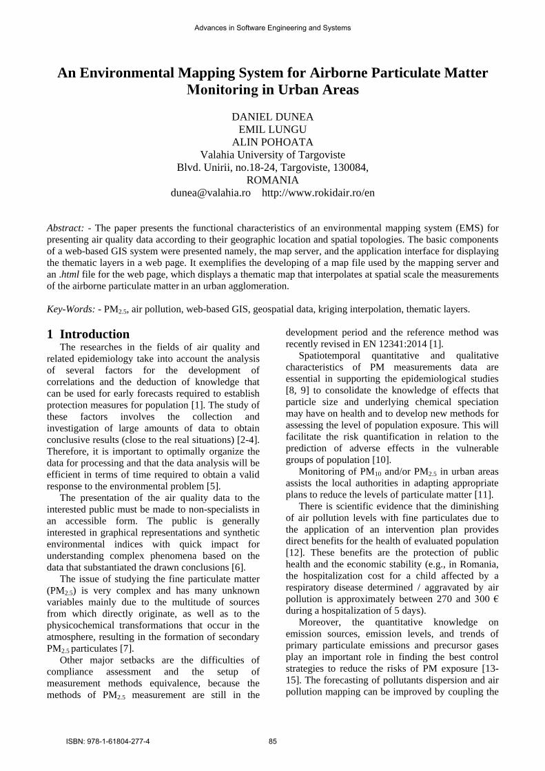
3.3 Creation of a map file A map file is a configuration file that is sent to the

mapserv.exe executable. This file defines the

relationships between the objects that are envisaged

to be displayed in the map. It indicates where the

data are located and defines how these data are

displayed (http://mapserver.org/mapfile/index.html).

Advances in Software Engineering and Systems

ISBN: 978-1-61804-277-4 89

A map file contains text that defines various objects

/properties introduced by labels such as LABEL,

LAYER, LEGEND, FONTSET, PROJECTION and

finished with END label. Based on the MAP object

that contains one or more LAYER objects, a

LAYER object is a combination of data along with a

set of styles.

Fig. 5 Flow of data processing to obtain the

concentration isolines using PM2.5 in-situ measured

data

The example below shows how to format the data of

interest using a map file type.

MAP

SIZE 600 400

SHAPEPATH "d:/data"

EXTENT -180 -89 180 89

FONTSET "fonts/fonts.list"

#IMAGECOLOR "#00000000"

OUTPUTFORMAT

NAME png

DRIVER AGG/PNG

MIMETYPE "image/png"

IMAGEMODE RGBA

TRANSPARENT ON

EXTENSION "png"

END

IMAGETYPE PNG

UNITS DD

WEB

IMAGEPATH

"/localhost/htdocs/tmp/"

IMAGEURL "/tmp/"

METADATA

"wms_enable_request" "*"

"wms_srs" "EPSG:4326

EPSG:3857"

"wms_feature_info_mime_type" "text/html"

"wms_format" "image/png"

"wms_title" "Rokidair

Demo"

"wms_onlineresource"

"http://localhost/wmsmap?"

END

END

PROJECTION

"init=epsg:4326"

END

#Circle symbol

SYMBOL

NAME 'CIRCLE'

TYPE ellipse

FILLED true

POINTS

1 1

END

END

LAYER

NAME PuncteM

TRANSPARENCY 100

TYPE POINT

PROJECTION

"init=epsg:4326" # WGS84

latlon

END

STATUS ON

DATA PuncteM

CLASS

NAME 'PuncteM'

STYLE

SYMBOL 'CIRCLE'

COLOR '#ff0000'

SIZE 10

END

TEXT

'[PntMasura]_Max:[MaxVal]_Med:[MedVal]'

LABEL

TYPE TRUETYPE

FONT arial-bold

SIZE 8

ANTIALIAS TRUE

POSITION UR

COLOR 0 0 255

WRAP "_"

END

END

END

LAYER

NAME 'PM25'

TYPE RASTER

DATA 'PM25.TIF'

PROCESSING "BANDS=1"

STATUS OFF

METADATA

'ows_title' 'PM25'

END

TRANSPARENCY 70

CLASS

EXPRESSION ([pixel] >= 0

AND [pixel] < 20)

STYLE

COLORRANGE 150 240

240 255 180 180

DATARANGE 0 20

RANGEITEM "pixel"

END #STYLE

END #end class

PROJECTION

"init=epsg:4326"

END

END

LAYER

NAME 'PM25Iso'

TYPE LINE

TRANSPARENCY 100

Advances in Software Engineering and Systems

ISBN: 978-1-61804-277-4 90

PROJECTION

"init=epsg:4326"

END

DATA PM25Iso

METADATA

'ows_title' 'PM25Iso'

END

STATUS ON

TRANSPARENCY 100

LABELITEM 'PM25'

CLASSITEM 'PM25'

CLASS

NAME 'iso'

EXPRESSION ( ([PM25] >= 0) AND

([PM25] <= 14) )

STYLE

WIDTH 1.96

COLOR 0 0 255

END

LABEL

FONT arial-bold

TYPE truetype

SIZE 8

COLOR 0 0 255

ANGLE AUTO

OFFSET -5 5

POSITION cc

FORCE true

ANTIALIAS true

PARTIALS true

END

END

END

END

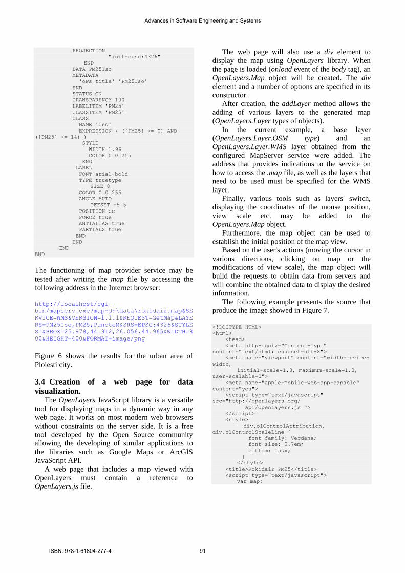
The functioning of map provider service may be

tested after writing the map file by accessing the

following address in the Internet browser:

http://localhost/cgi-

bin/mapserv.exe?map=d:\data\rokidair.map&SE

RVICE=WMS&VERSION=1.1.1&REQUEST=GetMap&LAYE

RS=PM25Iso,PM25,PuncteM&SRS=EPSG:4326&STYLE

S=&BBOX=25.978,44.912,26.056,44.965&WIDTH=8

00&HEIGHT=400&FORMAT=image/png Figure 6 shows the results for the urban area of

Ploiesti city.

3.4 Creation of a web page for data

visualization. The OpenLayers JavaScript library is a versatile

tool for displaying maps in a dynamic way in any

web page. It works on most modern web browsers

without constraints on the server side. It is a free

tool developed by the Open Source community

allowing the developing of similar applications to

the libraries such as Google Maps or ArcGIS

JavaScript API.

A web page that includes a map viewed with

OpenLayers must contain a reference to

OpenLayers.js file.

The web page will also use a div element to

display the map using OpenLayers library. When

the page is loaded (onload event of the body tag), an

OpenLayers.Map object will be created. The div

element and a number of options are specified in its

constructor.

After creation, the addLayer method allows the

adding of various layers to the generated map

(OpenLayers.Layer types of objects).

In the current example, a base layer

(OpenLayers.Layer.OSM type) and an

OpenLayers.Layer.WMS layer obtained from the

configured MapServer service were added. The

address that provides indications to the service on

how to access the .map file, as well as the layers that

need to be used must be specified for the WMS

layer.

Finally, various tools such as layers' switch,

displaying the coordinates of the mouse position,

view scale etc. may be added to the

OpenLayers.Map object.

Furthermore, the map object can be used to

establish the initial position of the map view.

Based on the user's actions (moving the cursor in

various directions, clicking on map or the

modifications of view scale), the map object will

build the requests to obtain data from servers and

will combine the obtained data to display the desired

information.

The following example presents the source that

produce the image showed in Figure 7.

<!DOCTYPE HTML>

<html>

<head>

<meta http-equiv="Content-Type"

content="text/html; charset=utf-8">

<meta name="viewport" content="width=device-

width,

initial-scale=1.0, maximum-scale=1.0,

user-scalable=0">

<meta name="apple-mobile-web-app-capable"

content="yes">

<script type="text/javascript"

src="http://openlayers.org/

api/OpenLayers.js ">

</script>

<style>

div.olControlAttribution,

div.olControlScaleLine {

font-family: Verdana;

font-size: 0.7em;

bottom: 15px;

}

</style>

<title>Rokidair PM25</title>

<script type="text/javascript">

var map;

Advances in Software Engineering and Systems

ISBN: 978-1-61804-277-4 91

Fig. 6 Image provided by the server based on the map file that interpolated the PM2.5

measurements in Ploiesti city

Fig. 7 Viewing the thematic map in browser showing the potential distribution of PM2.5

concentrations in Ploiesti city (isolines of 1 µg m-3 equidistance)

var lat =44.94133333;

var lon = 26.04;

function init() {

map = new OpenLayers.Map(

'map',{projection:

"EPSG:3857",displayProjection:

"EPSG:4326"});

map.addLayer(new OpenLayers.Layer.OSM(

"OSM layer"));

wmslyr = new OpenLayers.Layer.WMS(

"Statii",

"http://localhost/cgi-

bin/mapserv.exe?map=d:/data/rokidair.map",

{

layers: 'PM25Iso,PM25,PuncteM',

isBaseLayer: false,

transparent:true,

format:'image/png'

},

{

singleTile: true

}

);

map.addLayer(wmslyr);

map.setCenter(

new OpenLayers.LonLat(lon,

lat).transform(

new

OpenLayers.Projection("EPSG:4326"),

map.getProjectionObject()

), 14

);

map.addControl(new

OpenLayers.Control.MousePosition());

map.addControl(new

OpenLayers.Control.LayerSwitcher());

}

</script>

</head>

<body onload="init()">

<div id="map" style="width: 820px;

height: 500px"></div>

</body>

</html>

Advances in Software Engineering and Systems

ISBN: 978-1-61804-277-4 92

Fig. 8 Thematic map of the potential distribution of the

annual minimum PM10 concentration in Ploiesti city

Fig. 9 Thematic map of the potential distribution of the

annual average PM10 concentration in Ploiesti city

Figures 8, 9 and 10 shows examples of digital

maps obtained using the described technique by

interpolating the annual minimum, average and

maximum PM10 concentrations measured at 4

automated monitoring stations located in Ploiesti.

Such isolines must be checked for conformity using

in-situ measurements and dispersion modeling using

complex numerical models (e.g. Breeze® Aermod),

meteorology and topography.

Fig. 10 Thematic map of the potential distribution of the

annual maximum PM10 concentration in Ploiesti city

4 Conclusion We consider that the software programs involved

in the monitoring and/ or forecasting of air quality

should include in their structure an environmental

mapping system, even a simplified one, having air

pollutants dispersion capabilities to meet the criteria

required by the air quality planning in the region of

interest.

The presented case study provides a simple and

versatile solution to develop such instruments. The

resulted application represents a component in the

future ROKIDAIR geoportal, which will provide

intelligent support for the children’s health

management under the impact of air quality

stressors and pressures. If a pollution episode is

expected, supplemental details may be requested

regarding the probable source or PM2.5 speciation to

provide expert advice to the public in relation to

possible health effects or to help with effective

measures for reducing the impact of the episode.

The final system will be developed on an open-

GIS platform having the versatility, flexibility and

ability to easily develop software codes. It will

integrate a PM forecasting tool based on artificial

intelligence algorithms such as predictive data

mining and hybrid neural networks [8, 20].

All contained data resulted from statistical

processing, numerical modeling or data forecasting

will be adapted for consultation on smart phones

and other portable devices.

Advances in Software Engineering and Systems

ISBN: 978-1-61804-277-4 93

ACKNOWLEDGEMENTS The research leading to these results has received

funding from EEA Financial Mechanism 2009 -

2014 under the project ROKIDAIR “Towards a

better protection of children against air pollution

threats in the urban areas of Romania” contract

no. 20SEE/30.06.2014.

References:

[1] Iordache Ş., Dunea D. (Eds.), Evaluation

methods of air pollution with particulate matter

effects on children’s health, Ed. Matrix Rom,

Bucharest, pp. 476, 2014.

[2] Iordache Ş., Dunea D., Cross-spectrum analysis

applied to air pollution time series from several

urban areas of Romania, Environmental

Engineering and Management Journal, 12(4),

2013, pp. 677-684.

[3] Hajek P., Olej V., Air quality indices and their

modelling by hierarchical Fuzzy Inference

Systems, WSEAS Transactions on Environment

and Development, Vol. 5, Issue 10, 2009, pp.

661-672.

[4] Dunea D., Iordache Ş., Alexandrescu D.C.,

Dincă N., Screening the Weekdays/Weekend

Patterns of Air Pollutant Concentrations

Recorded in Southeastern Romania,

Environmental Engineering and Management

Journal, 13(12), 2014.

[5] Dunea D., Iordache Ş., Oprea M., Savu T.,

Pohoaţă A., Lungu E., A relational database

structure for linking air pollution levels with

children’s respiratory illnesses, Bulletin

UASVM CN, 71(2), 2014, pp. 205-213.

[6] AQEG, Fine Particulate Matter (PM2.5) in the

United Kingdom, Defra, London, 2012.

[7] World Health Organization, Exposure to air

pollution (particulate matter) in outdoor air,

Copenhagen, WHO Regional Office for

Europe, ENHIS Factsheet 3.3, 2011.

[8] Dunea D., Iordache Ş., Pohoaţă A., Multiple

characterizations of urban air pollution time

series using a wavelet feedforward neural

network integrative approach, Proceedings

ITISE 2014, International work-conference on

Time Series, Granada, Vol.2, 2014, pp. 804-

815.

[9] Dunea D., Oprea M., Lungu E., Comparing

statistical and neural network approaches for

urban air pollution time series analysis,

Proceedings of the 27th IASTED International

conference on “Modelling, Identification and

Control” (ed. L. Bruzzone), Acta Press, 2008,

pp. 93-98.

[10] Moshammer H. et al., Air pollution: A threat to

the health of our children, ACTA Paediatrica,

95, Suppl 453, DOI: 10.1080/

08035320600886620, 2006, pp. 93-105.

[11] Iordache Ş., Dunea D., Ianache C., Predescu L.,

Dumitru D., Air quality characterization in

Ploiesti urban area affected by industrial and

traffic pollution, Bulletin UASVM CN, 71(2),

2014, pp. 219-225.

[12] Neuberger M., Schimek M.G., Horak Jr. F.,

Moshammer H., Kundi M., Frischer T.,

Gomiscek B., Puxbaum H., Hauck H.,

AUPHEP-Team, Acute effects of particulate

matter on respiratory diseases, symptoms and

functions: epidemiological results of the

Austrian Project on Health Effects of

Particulate Matter (AUPHEP), Atmospheric

Environment 38, 2004, pp. 3971–3981.

[13] Liu H-Y., Skjetne E., Kobernus M., Mobile

phone tracking: in support of modelling traffic-

related air pollution contribution to individual

exposure and its implications for public health

impact assessment, Environmental Health,

12:93, 2013.

[14] Rahman S.M., Khondaker A.N., Abdel-Aal R.,

Self organizing ozone model for Empty Quarter

of Saudi Arabia: Group method data handling

based modeling approach, Atmospheric

Environment, Vol. 59, 2012, pp. 398–407.

[15] Rivas I., Viana M., Moreno T., Pandolfi M.,

Amato F., Reche C., Bouso L., Alvarez-

Pedrerol M., Alastuey A., Sunyer J., Querol X.,

Child exposure to indoor and outdoor air

pollutants in schools in Barcelona, Spain,

Environment International, 69, 2014, pp. 200–

212.

[16] Enkhtur B., Geostatistical modelling and

mapping of air pollution, M.Sc. Thesis,

University of Twente, Enschede, 2013.

[17] Nicolescu C., Gorghiu G., Dunea D.,

Buruleanu L., Moise V., Mapping Air Quality:

An Assessment of the Pollutants Dispersion in

Inhabited Areas to Predict and Manage

Environmental Risks, WSEAS Transactions on

Environment and Development, Vol. 4, Issue

12, pp. 1078-1088.

[18] Romanian National Network for Air Quality

Monitoring (RNMCA) – http://calitateaer.ro/

[19] AirBase: public air quality database [online

database], Copenhagen, European Environment

Agency,http://www.eea.europa.eu/themes/air/ai

rbase

[20] Oprea M., INTELLEnvQ-Air: An Intelligent

System for Air Quality Analysis in Urban

Regions, International Journal of Artificial

Intelligence, 9(A12), 2012, pp. 106-122.

Advances in Software Engineering and Systems

ISBN: 978-1-61804-277-4 94