an equivalence relation for local path sets

An Equivalence Relation for Local Path Sets

Ross A. Knepper, Siddhartha S. Srinivasa, and Matthew T. Mason

Abstract We propose a novel enhancement to the task of collision-testing a set oflocal paths. Our approach circumvents expensive collision-tests, yet it declares acontinuum of paths collision-free by exploiting both the structure of paths and theoutcome of previous tests. We define a homotopy-like equivalence relation amonglocal paths and provide algorithms to (1) classify paths based on equivalence, and(2) implicitly collision-test up to 90% of them. We then prove both correctness andcompleteness of these algorithms before providing experimental results showing aperformance increase up to 300%.

1 Introduction

Planning bounded-curvature paths for mobile robots is an NP-hard problem [22].Many nonholonomic mobile robots thus rely on hierarchical planning architec-tures [1, 13, 19], which split responsibility between at least two layers (Fig. 1): aslow global planner and fast local planner. We focus here on the local planner (Alg. 1and Alg. 2), which iterates in a tight loop: searching through a set of paths and se-lecting the best path for execution. During each loop, the planner tests many pathsbefore making an informed decision. The bottleneck in path testing is collision-testing [24]. In this paper, we introduce a novel approach that delivers a significantincrease in path set collision-testing performance by exploiting the fundamental ge-ometric structure of paths.

We introduce an equivalence relation intuitively resembling the topological no-tion of homotopy. Two paths are path homotopic if a continuous, collision-free de-formation with fixed start and end points exists between them [20]. Like any path

Ross A. Knepper and Matthew T. MasonCarnegie Mellon University, 5000 Forbes Ave, Pittsburgh PA, e-mail: {rak,mason}@ri.cmu.edu

Siddhartha S. SrinivasaIntel Labs Pittsburgh, 4720 Forbes Ave, Pittsburgh, PA e-mail: [email protected]

1

2 Ross A. Knepper, Siddhartha S. Srinivasa, and Matthew T. Mason

Fig. 1 An example hier-archical planning scenario.The local planner’s path setexpands from the robot, atcenter, and feeds commandsto the robot based on the bestpath that avoids obstacles(black squares). The chosenlocal path (green) and globalpath (red) combine to form aproposed path to the goal.

equivalence relation, homotopy partitions paths into equivalence classes. Differenthomotopy classes make fundamentally different choices about their route amongstobstacles. However, two mobile robot concepts translate poorly into homotopy the-ory: limited sensing and constrained action.

The robot may lack a complete workspace map, which must instead be con-structed from sensor data. Since robot perception is limited by range and occlusion,a robot’s understanding of obstacles blocking its movement evolves with its vantagepoint. A variety of sensor-based planning algorithms have been developed to handlesuch partial information. Obstacle avoidance methods, such as potential fields [12],are purely reactive. The bug algorithm [18], which generates a path to the goal us-ing only a contact sensor, is complete in 2D. Choset and Burdick [5] present thehierarchical generalized Voronoi graph, a roadmap with global line-of-sight acces-sibility that achieves completeness in higher dimensions using range readings of theenvironment.

If a robot is tasked to perform long-range navigation, then it must plan a paththrough unsensed regions. A low-fidelity global planner generates this path becausewe prefer to avoid significant investment in this plan, which will likely be invalidatedlater. Path homotopy, in the strictest sense, requires global knowledge of obstaclesbecause homotopy equivalent paths must connect fixed start and goal points.

Relaxing the endpoint requirement avoids reasoning about the existence of far-away, unsensed obstacles. Naively relaxing a fixed endpoint, our paths might bepermitted to freely deform around obstacles, making all paths equivalent. To re-store meaningful equivalence classes, we propose an alternate constraint based onpath shape. This is in keeping with the nonholonomic constraints that limit mo-bile robots’ action. Laumond [15] first highlighted the importance of nonholonomicconstraints and showed that feasible paths exist for a mobile robot with such con-straints. Barraquand and Latombe [2] created a grid-based planner that innatelycaptures these constraints. LaValle and Kuffner [17] proposed the first planner toincorporate both kinodynamic constraints and random sampling. In contrast to non-holonomic constraints, true homotopy forbids restrictions on path shape; two pathsare equivalent if any path deformation—however baroque—exists between them.By restricting our paths to bounded curvature, we represent only feasible motionswhile limiting paths’ ability to deform around obstacles. The resulting set of pathequivalence classes is of immediate importance to the planner (Fig. 2). The number

An Equivalence Relation for Local Path Sets 3

Fig. 2 left: Paths from a few distinct homotopy classes between the robot and the goal. The dis-tinctions between some classes require information that the robot has not yet sensed (the dark areais out of range or occluded). middle: With paths restricted to the sensed area, they may freely de-form around visible obstacles. right: After restricting path shape to conform to motion constraints,we get a handful of equivalence classes that are immediately applicable to the robot.

of choices represented by these local equivalence classes relates to Farber’s topo-logical complexity of motion planning [6].

Equivalence classes have been employed in various planners. In task planning, re-cent work has shown that equivalence classes of actions can be used to eliminate re-dundant search [7]. In motion planning, path equivalence often employs homotopy.A recent paper by Bhattacharya, Kumar, and Likhachev [3] provides a techniquebased on complex analysis for detecting homotopic equivalence among paths in 2D.Two papers employing equivalence classes to build probabilistic roadmaps [11] areby Schmitzberger, et al. [25] and Jaillet and Simeon [10]. The latter paper departsfrom true homotopy by proposing the visibility deformation, a simplified alternativeto homotopic equivalence based on line-of-sight visibility between paths.

Our key insight is that local path equivalence is an expressive and powerful toolthat reveals shared outcomes in collision-testing. Specifically, two equivalent neigh-boring paths cover some common ground in the workspace, and between them liesa continuum of covered paths. We develop the mathematical foundations to detectequivalence relations among all local paths based on a finite precomputed path set.We then utilize these tools to devise efficient algorithms for detecting equivalenceand implicitly collision-testing local paths.

The remainder of the paper is organized as follows. We provide an implementa-tion of the basic algorithm in Section 2 and present the fast collision-testing tech-nique. Section 3 then explores the theoretical foundations of our path equivalencerelation. Section 4 provides some experimental results.

2 Algorithms

In this section, we present three algorithms: path set generation, path classification,and implicit path collision-testing. All of the algorithms presented here run in poly-nomial time. Throughout this paper, we use lowercase p to refer to a path in theworkspace, while P is a set of paths (each one a point in path space).


Algorithm 1 Test All Paths(w, P)Input: w – a costmap object; P – a fixed set of pathsOutput: P f ree, the set of paths that passed collision test1: P f ree← /02: while time not expired and untested paths remain do // test paths for 0.1 seconds3: p← Get Next Path(P)4: collision← w.Test Path(p) // collision is boolean5: if not collision then6: P f ree←P f ree∪{p} // non-colliding path set7: return P f ree

Algorithm 2 Local Planner Algorithm(w, x, h, P)Input: w – a costmap object; x – initial state; h – a heuristic function for selecting a path to execute;

P – a fixed set of pathsOutput: Moves the robot to the goal if possible1: while not at goal and time not expired do2: P f ree← Test All Paths(w,x,P)3: j← h.Best Path(x,P f ree)4: Execute Path On Robot( j)5: x← Predict Next State(x, j)

Definition 1. Path space is a metric space (P,µ) in which the distance between apair of paths in P is defined by metric µ . Paths can vary in shape and length. ut

2.1 Path Set Generation

We use the greedy path set construction technique of Green and Kelly [8], outlinedin Alg. 3. The algorithm iteratively builds a path set PN by drawing paths from adensely-sampled source path set, X. During step i, it selects the path p ∈ X thatminimizes the dispersion of Pi = Pi−1∪{p}. Borrowing from Niederreiter [21]:

Definition 2. Given a bounded metric space (X,µ) and point set P = {x1, . . . ,xN} ∈X, the dispersion of P in X is defined by

δ (P,X) = supx∈X

minp∈P

µ(x, p) . ut (1)

The dispersion of P in X equals the radius of the biggest open ball in X containingno points in P. By minimizing dispersion, we ensure that there are no large voidsin path space. Thus, dispersion reveals the quality of P as an “approximation” ofX because it guarantees that for any x ∈ X, there is some point p ∈ P such thatµ(x, p)≤ δ (P,X).

The Green-Kelly algorithm generates a sequence of path sets Pi, for i∈{1, . . . ,N},that has monotonically decreasing dispersion. Alg. 1 searches paths in this order atruntime, thus permitting early termination while retaining near-optimal results. Note


that while the source set X is of finite size—providing a lower bound on dispersionat runtime—it can be chosen with arbitrarily low dispersion a priori.

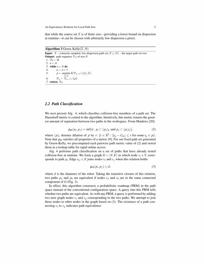
Algorithm 3 Green Kelly(X, N)Input: X – a densely-sampled, low-dispersion path set; N ≤ |X| – the target path set sizeOutput: path sequence PN of size N1: P0← /02: n← 03: while n < N do4: n← n+15: p← argmin

x∈Xδ (Pn−1∪{x},X)

6: Pn←Pn−1∪{p}7: return PN

2.2 Path Classification

We next present Alg. 4, which classifies collision-free members of a path set. TheHausdorff metric is central to the algorithm. Intuitively, this metric returns the great-est amount of separation between two paths in the workspace. From Munkres [20]:

µH(pi, p j) = inf{ε : pi ⊂ (p j)ε and p j ⊂ (pi)ε}, (2)

where (p)r denotes dilation of p by r: {t ∈ R2 : ‖tp− t‖L2 ≤ r for some tp ∈ p}.Note that µH satisfies all properties of a metric [9]. For our fixed path set generatedby Green-Kelly, we precomputed each pairwise path metric value of (2) and storedthem in a lookup table for rapid online access.

Alg. 4 performs path classification on a set of paths that have already testedcollision-free at runtime. We form a graph G = (V,E) in which node vi ∈ V corre-sponds to path pi. Edge ei j ∈ E joins nodes vi and v j when this relation holds:

µH(pi, p j)≤ d, (3)

where d is the diameter of the robot. Taking the transitive closure of this relation,two paths pa and pb are equivalent if nodes va and vb are in the same connectedcomponent of G (Fig. 3).

In effect, this algorithm constructs a probabilistic roadmap (PRM) in the pathspace instead of the conventional configuration space. A query into this PRM tellswhether two paths are equivalent. As with any PRM, a query is performed by addingtwo new graph nodes vs and vg corresponding to the two paths. We attempt to jointhese nodes to other nodes in the graph based on (3). The existence of a path con-necting vs to vg indicates path equivalence.


Fig. 3 A simple path set,in which obstacles (black)eliminate colliding paths.The collision-free path sethas three equivalence classes(red, green, and blue). In thecorresponding graph repre-sentation, at right, adjacentnodes represent proximalpaths. Connected componentsindicate equivalence classesof paths.

Algorithm 4 Equivalence Classes(P f ree, d)Input: P f ree – a set of safe, appropriate paths; d – the diameter of the robotOutput: D – a partition of P f ree into equivalence classes (a set of path sets)1: Let G = (V,E)← ( /0, /0)2: D← /03: for all pi ∈P f ree do // This loop discovers adjacency4: V.add(pi) // Add a graph node corresponding to path pi5: for all p j ∈V \{pi} do6: if µH(pi, p j) < d then7: E.add(i, j) // Connect nodes i and j with an unweighted edge8: S←P f ree9: while S 6= /0 do // This loop finds the connected components

10: C← /011: p← a member of S12: L←{p} // List of nodes to be expanded in this class13: while L 6= /0 do14: p← a member of L15: C←C∪{p} // Commit p to class16: S← S\{p}17: L← (L∪V.neighbors(p))∩S18: D← D∪{C}19: return D

2.3 Implicit Path Safety Test

There is an incessant need in motion planning to accelerate collision-testing, whichmay take 99% of total CPU time [24]. During collision-testing, the planner mustverify that a given swath is free of obstacles.

Definition 3. A swath is the workspace area of ground or volume of space sweptout as the robot traverses a path. ut

Definition 4. We say a path is safe if its swath contains no obstacles. ut

In testing many swaths of a robot passing through space, most planners ef-fectively test the free workspace many times by testing overlapping swaths. Wemay test a path implicitly at significant computational savings by recalling recent


collision-testing outcomes. We formalize the idea in Alg. 5, which is designed to beinvoked from Alg. 1, line 4 in lieu of the standard path test routine.

The implicit collision-test condition resembles the neighbor condition (3) usedby Alg. 4, but it has an additional “Is Between” check, which indicates that theswath of the path under test is covered by two collision-free neighboring swaths.The betweenness trait can be precomputed and stored in a lookup table. Given a setof safe paths, we can quickly discover whether any pair covers the path under test.Experimental results show that this algorithm allows us to test up to 90% of pathsimplicitly, thus increasing the path evaluation rate by up to 300% in experiments.

Algorithm 5 Test Path Implicit(p, w, S, d)Input: p is a path to be testedInput: w is a costmap object // used as a backup when path cannot be implicitly testedInput: S is the set of safe paths found so farInput: d is the diameter of the robot1: for all pi, p j ∈ S such that µH(pi, p j)≤ d do2: if p.Is Between(pi, p j) then // p’s swath has been tested previously3: s f ← p.Get End Point()4: collision← w.Test Point(s f ) // endpoint may not be covered by swaths5: return collision6: return w.Test Path(p) // Fall back to explicit path test

3 Foundations

In this section, we establish the foundations of an equivalence relation on pathspace based on continuous deformations between paths. We then provide correct-ness proofs for our algorithms for classification and implicit collision-testing.

We assume a kinematic description of paths. All paths are parametrized bya shared initial pose, shared fixed length, and individual curvature function. Letκi(s) describe the curvature control of path i as a function of arc length, withmax0≤s≤s f |κi(s)| ≤ κmax. Typical expressions for κi include polynomials, piecewiseconstant functions, and piecewise linear functions. The robot motion produced bycontrol i is a feasible path given by θi

xiyi

=

κicosθisinθi

. (4)

Definition 5. A feasible path has bounded curvature (implying C1 continuity) andfixed length. The set F(s f ,κmax) contains all feasible paths of length s f and curva-ture |κ(s)| ≤ κmax. ut


Fig. 4 At top: several ex-ample paths combining dif-ferent values of v and w.Each path pair obeys (3).The value of v affects the“curviness” allowed in paths,while w affects their length.At bottom: this plot, gen-erated numerically, approx-imates the set of appropri-ate choices for v and w.The gray region at top rightmust be avoided, as we showin Lemma 2. Such choiceswould permit an obstacle tooccur between two safe pathsthat obey (3). A path whosevalues fall in the white regionis called an appropriate path.

0

0.2

0.4

0.6

0.8

1

0 0.2 0.4 0.6 0.8 1

w

v

1

*

*

*v=0 w=1 v=1 w=0.17 v=0.5 w=0.5 v=1 w=1

*

w

v

0.8

0.6

0.4

0.2

00 0.2 0.4 0.6 0.8 1

Path setin Fig. 1

3.1 Properties of Paths

In this section, we establish a small set of conditions under which we can quickly de-termine that two paths are equivalent. We constrain path shape through two dimen-sionless ratios relating three physical parameters. We may then detect equivalencethrough a simple test on pairs of paths using the Hausdorff metric.

These constraints ensure a continuous deformation between neighboring pathswhile permitting a range of useful actions. Many important classes of action setsobey these general constraints, including the line segments common in RRT [17] andPRM planners, as well as constant curvature arcs. Fig. 1 illustrates a more expressiveaction set [13] that adheres to our constraints.

The three physical parameters are: d, the diameter of the robot; s f , the length ofeach path; and rmin, the minimum radius of curvature allowed for any path. Notethat 1/rmin = κmax, the upper bound on curvature. For non-circular robots, d reflectsthe minimal cross-section of the robot’s swath sweeping along a path. We expressrelationships among the three physical quantities by two dimensionless parameters:

v =d

rminw =

s f

2πrmin.

We only compare paths with like values of v and w. Fig. 4(top) provides some intu-ition on the effect of these parameters on path shape. Due to the geometry of paths,only certain choices of v and w are appropriate.


Definition 6. An appropriate path is a feasible path conforming to appropriate val-ues of v and w from the proof of Lemma 2. Fig. 4 previews the permissible values.

When the condition in (3) is met, the two paths’ swaths overlap, resulting in acontinuum of coverage between the paths. This coverage, in turn, ensures the exis-tence of a continuous deformation, as we show in Theorem 1, but first we formallydefine a continuous deformation between paths.

Definition 7. A continuous deformation between two safe, feasible paths pi and p jin F(s f ,κmax) is a continuous function f : [0,1]→ F(s−f ,κ+

max), with s−f slightly lessthan s f and κ+

max slightly more than κmax. f (0) is the initial interval of pi, and f (1)is the initial interval of p j, both of length s−f . We write pi ∼ p j to indicate thata continuous deformation exists between paths pi and p j, and they are thereforeequivalent. ut

The length s−f depends on v and w, but for typical values, s−f is fully 95–98% ofs f . For many applications, this is sufficient, but an application can quickly test theremaining path length if necessary. Nearly all paths f (c) are bounded by curvatureκmax, but it will turn out that in certain geometric circumstances, the maximumcurvature through a continuous deformation is up to κ+

max = 43 κmax.

Definition 8. Two safe, feasible paths that define a continuous deformation arecalled guard paths because they protect the intermediate paths. ut

In the presence of obstacles, it is not trivial to determine whether a continuousdeformation is safe, thus maintaining equivalency. Rather than trying to find a defor-mation between arbitrary paths, we propose a particular condition under which weshow that a bounded-curvature, fixed-length, continuous path deformation exists,

µH(p1, p2)≤ d =⇒ p1 ∼ p2. (5)

This statement, which we prove in the next section, is the basis for Alg. 4 and Alg. 5.The overlapping swaths of appropriate paths p1 and p2 cover a continuum of inter-mediate swaths between the two paths. Eqn. (5) is a proper equivalence relationbecause it possesses each of three properties:

• reflexivity. µH(p, p) = 0; p is trivially deformable to itself.• symmetry. The Hausdorff metric is symmetric.• transitivity. Given µH(p1, p2) ≤ d and µH(p2, p3) ≤ d, a continuous deforma-

tion from p1 to p3 passes through p2.

3.2 Equivalence Relation

Having presented the set of conditions under which (5) holds, we now prove thatthey are sufficient to ensure the existence of a continuous deformation between two


Fig. 5 Paths pi, p j, and peform boundary B. Its interior,I, contains all paths in thecontinuous deformation frompi to p j .

I I pepipj

neighboring paths. Our approach to the proof will be to first describe a feasiblecontinuous deformation, then show that paths along this deformation are safe.

Given appropriate guard paths pi and p j with common origin, let pe be the short-est curve in the workspace connecting their endpoints without crossing either path(pe may pass through obstacles). The closed path B = pi ∪ p j ∪ pe creates one ormore closed loops (the paths may cross each other). By the Jordan curve theorem,each loop partitions R2 into two sets, only one of which is compact. Let I, the inte-rior, be the union of these compact regions with B, as in Fig. 5.

Definition 9. A path pc is between paths pi and p j if pc ⊂ I. ut

Lemma 1. Given appropriate paths pi, p j ⊂F(s f ,κmax) with µH(pi, p j)≤ d, a pathsequence exists in the form of a feasible continuous deformation between pi and p j.

Proof. We provide the form of a continuous deformation from pi to p j such thateach intermediate path is between them. With t a workspace point and p a path, let

γ(t, p) = inf{ε : t ∈ (p)ε} (6)

g(t) =

{[0,1] if γ(t, pi) = γ(t, p j) = 0{

γ(t,pi)γ(t,pi)+γ(t,p j)

}otherwise, (7)

where g(t) is a set-valued function to accommodate intersecting paths. Each levelset g(t) = c for c ∈ [0,1] defines a weighted generalized Voronoi diagram (GVD)forming a path as in Fig. 6. We give the form of a continuous deformation usinglevel sets g−1(c); each path is parametrized starting at the origin and extending fora length s−f in the direction of pe. Let us now pin down the value of s−f . Every pointti on pi forms a line segment projecting it to its nearest neighbor t j on p j (and viceversa). Their collective area is shown in Fig. 7. Eqn. (3) bounds each segment’slength at d. s−f is the greatest value such that no intermediate path of length s−fdeparts from the region covered by these projections.

For general shapes in R2, the GVD forms a set of curves meeting at branchingpoints [23]. In this case, no GVD cusps or branching points occur in any interme-diate path. Since d < rmin, no center of curvature along either guard path can fall inI [4]. Therefore, each level set defines a path through the origin.

Each path’s curvature function is piecewise continuous and everywhere bounded.A small neighborhood of either guard path approximates constant curvature. A GVDcurve generated by two constant-curvature sets forms a conic section [27]. Table 1reflects that the curvature of pc is everywhere bounded with the maximum possiblecurvature being bounded by 4

3 κmax. For the full proofs, see [14]. ut


Fig. 6 In a continuous de-formation between paths piand p j , as defined by the levelsets of (7), each path takesthe form of a weighted GVD.Upper bounds on curvaturevary along the deformation,with the maximum bound of43 κmax occurring at the medialaxis of the two paths.

pi

pj

point of maximum curvature

pepc

pi

pj

Fig. 7 Hausdorff coverage (overlapping red and blue shapes in center) is a conservative approxi-mation of swath coverage (gray). The Hausdorff distance between paths pi and p j is equal to themaximum-length projection from any point on either path to the closest point on the opposite path.Each projection implies a line segment. The set of projections from the top line (blue) and bottomline (red) each cover a solid region between the paths. These areas, in turn, cover a slightly shorterintermediate path pc, in white, with its swath in cyan. This path’s length, s−f is as great as possiblewhile remaining safe, with its swath inside the gray area.

Table 1 Conic sections form the weighted Voronoi diagram. κ1 and κ2 represent the curvatures ofthe two guard paths, with κ1 the lesser magnitude. Let κm = max(|κ1|, |κ2|). For details, see [14].

Type Occurrence Curvature bounds of intermediate pathsline κ1 =−κ2 |κ| ≤ κmparabola κ1 = 0,κ2 6= 0 |κ| ≤ κmhyperbola κ1κ2 < 0,κ1 6=−κ2 |κ| ≤ κmellipse κ1κ2 > 0 |κ|< 4

3 κm

Lemma 2. Given safe, appropriate guard paths pi, p j ∈ F(s f ,κmax) separated byµH(pi, p j)≤ d, any path pc ⊂ F(s−f , 4

3 κmax) between them is safe.

Proof. We prove this lemma by contradiction. Assume an obstacle lies between piand p j. We show that this assumption imposes lower bounds on v and w. We thenconclude that for lesser values of v and w, no such obstacle can exist.

Let sl(p,d) = {t ∈ R2, tp = nn(t, p) : tpt ⊥ p and ‖t− tp‖L2 ≤ d2} define a con-

servative approximation of a swath, obtained by sweeping a line segment of lengthd with its center along the path. tpt is the line segment joining tp to t and nn(t, p)is the nearest neighbor of point t on path p. The two swaths form a safe region,U = sl(pi,d)∪ sl(p j,d).

Suppose that U contains a hole, denoted by the set h, which might contain anobstacle. Now, consider the shape of the paths that could produce such a hole. Be-


(a)

pih pj

h

pje p

ie

h

(b)

pjh

pie

hs

D

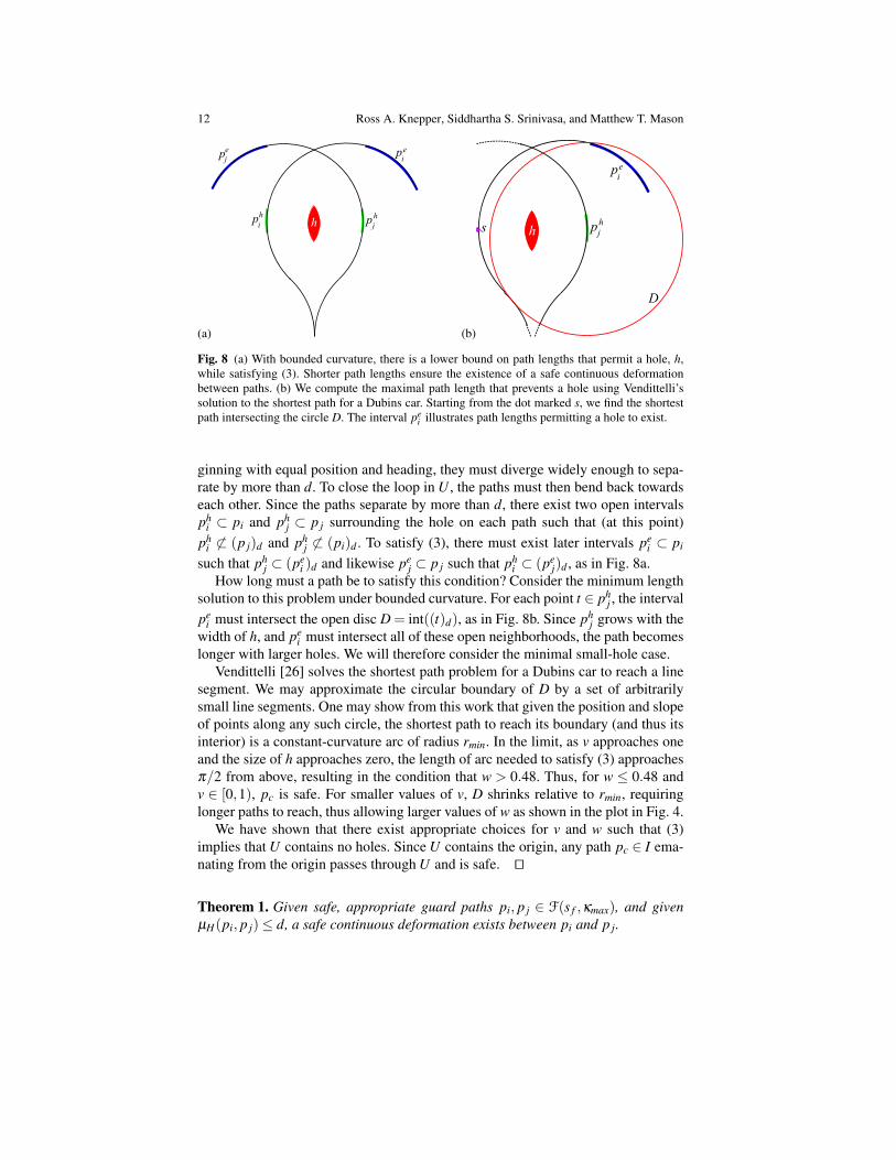
Fig. 8 (a) With bounded curvature, there is a lower bound on path lengths that permit a hole, h,while satisfying (3). Shorter path lengths ensure the existence of a safe continuous deformationbetween paths. (b) We compute the maximal path length that prevents a hole using Vendittelli’ssolution to the shortest path for a Dubins car. Starting from the dot marked s, we find the shortestpath intersecting the circle D. The interval pe

i illustrates path lengths permitting a hole to exist.

ginning with equal position and heading, they must diverge widely enough to sepa-rate by more than d. To close the loop in U , the paths must then bend back towardseach other. Since the paths separate by more than d, there exist two open intervalsph

i ⊂ pi and phj ⊂ p j surrounding the hole on each path such that (at this point)

phi 6⊂ (p j)d and ph

j 6⊂ (pi)d . To satisfy (3), there must exist later intervals pei ⊂ pi

such that phj ⊂ (pe

i )d and likewise pej ⊂ p j such that ph

i ⊂ (pej)d , as in Fig. 8a.

How long must a path be to satisfy this condition? Consider the minimum lengthsolution to this problem under bounded curvature. For each point t ∈ ph

j , the intervalpe

i must intersect the open disc D = int((t)d), as in Fig. 8b. Since phj grows with the

width of h, and pei must intersect all of these open neighborhoods, the path becomes

longer with larger holes. We will therefore consider the minimal small-hole case.Vendittelli [26] solves the shortest path problem for a Dubins car to reach a line

segment. We may approximate the circular boundary of D by a set of arbitrarilysmall line segments. One may show from this work that given the position and slopeof points along any such circle, the shortest path to reach its boundary (and thus itsinterior) is a constant-curvature arc of radius rmin. In the limit, as v approaches oneand the size of h approaches zero, the length of arc needed to satisfy (3) approachesπ/2 from above, resulting in the condition that w > 0.48. Thus, for w ≤ 0.48 andv ∈ [0,1), pc is safe. For smaller values of v, D shrinks relative to rmin, requiringlonger paths to reach, thus allowing larger values of w as shown in the plot in Fig. 4.

We have shown that there exist appropriate choices for v and w such that (3)implies that U contains no holes. Since U contains the origin, any path pc ∈ I ema-nating from the origin passes through U and is safe. ut

Theorem 1. Given safe, appropriate guard paths pi, p j ∈ F(s f ,κmax), and givenµH(pi, p j)≤ d, a safe continuous deformation exists between pi and p j.


Proof. Lemma 1 shows that (7) gives a continuous deformation between paths piand p j such that each intermediate path pc ⊂ I is feasible. Lemma 2 shows that anysuch path is safe. Therefore, a continuous deformation exists between pi and p j.This proves the validity of the Hausdorff metric as a test for path equivalence. ut

3.3 Resolution Completeness of Path Classifier

In this section, we show that Alg. 4 is resolution complete. Resolution complete-ness commonly shows that for a sufficiently high discretization of each dimensionof the search space, the planner finds a path exactly when one exists in the contin-uum space. We instead show that for a sufficiently low dispersion in the infinite-dimensional path space, the approximation given by Alg. 4 has the same connectiv-ity as the continuum safe, feasible path space.

Let F be the continuum feasible path space and F f ree ⊂ F be the set of safe,feasible paths. Using the Green-Kelly algorithm, we sample offline from F a pathsequence P of size N. At runtime, using Alg. 1, we test members of P in order todiscover a set P f ree ⊂ P of safe paths.

The following lemma is based on the work of LaValle, Branicky, and Linde-mann [16], who prove resolution completeness of deterministic roadmap (DRM)planners, which are PRM planners that draw samples from a low-dispersion, deter-ministic source. Since we use a deterministic sequence provided by Green-Kelly,the combination of Alg. 1 and 4 generates a DRM in path space.

Lemma 3. For any given configuration of obstacles and any path set PN generatedby the Green-Kelly algorithm, there exists a sufficiently large N such that any twopaths pi, p j ∈ P f ree are in the same connected component of F f ree if and only ifAlg. 4 reports that pi ∼ p j.

Proof. LaValle, et al. [16], show that by increasing N, a sufficiently low dispersioncan be achieved to make a DRM complete in any given C-Space. By an identicalargument, given a continuum connected component C ⊂ F f ree, all sampled pathsin C∩PN are in a single partition of D. If q is the radius of the narrowest corridorin C, then for dispersion δN < q, our discrete approximation exactly replicates theconnectivity of the continuum freespace. ut

Lemma 4. Under the same conditions as in Lemma 3, there exists a sufficientlylarge N such that for any continuum connected component C⊂ F f ree, Alg. 1 returnsa P f ree such that P f ree∩C 6= /0. That is, every component in F f ree has a correspond-ing partition returned by Alg. 4.

Proof. Let Br be the largest open ball of radius r in C. When δN < r, Br must containsome sample p∈P. Since C is entirely collision-free, p∈P f ree. Thus, for dispersionless than r, P f ree contains a path in C. ut


There exists a sufficiently large N such that after N samples, P has achieveddispersion δN < min(q,r), where q and r are the dispersion required by Lemmas 3and 4, respectively. Under such conditions, a bijection exists between the connectedcomponents of P f ree and F f ree.

Theorem 2. Let D = {D1| . . . |Dm} be a partition of P f ree as defined by Alg. 4. LetC = {C1| . . . |Cm} be a finite partition of the continuum safe, feasible path space intoconnected components. A bijection f : D→C exists such that Di ⊂ f (Di).

Proof. Lemma 3 establishes that f is one-to-one, while Lemma 4 establishes that fis onto. Therefore, f is bijective. This shows that by sampling at sufficiently highdensity, we can achieve an arbitrarily good approximation of the connectedness ofthe continuum set of collision-free paths in any environment. ut

Theorem 3. A path interval p may be implicitly tested safe if it is between pathspi and p j such that µH(pi, p j) ≤ d and a small region at the end of pc has beenexplicitly tested.

Proof. By Lemma 2, the initial interval of pc is safe because its swath is coveredby the swaths of the guard paths. Since the small interval at the end of pc has beenexplicitly tested, the whole of pc is collision-free. ut

4 Results

We briefly summarize some experimental results involving equivalence class detec-tion and implicit path collision-testing. All tests were performed in simulation onplanning problems of the type described in [13].

Path classification imposes a computational overhead due to the cost of searchingcollision-free paths. Collision rate in turn relates to the density of obstacles in theenvironment. The computational overhead of our classification implementation isnearly 20% in an empty environment but drops to 0.3% in dense clutter. However,implicit collision-testing more than compensates for this overhead.

Fig. 9 shows the effect of implicit path testing on total paths tested in the absenceof obstacles. As the time limit increases, the number of paths collision-tested un-der the traditional algorithm increases linearly at a rate of 8,300 paths per second.With implicit testing, the initial test rate over small time limits (thus small path setsizes) is over 22,500 paths per second. The marginal rate declines over time dueto the aforementioned overhead, but implicit path testing still maintains its speedadvantage until the entire 2,401-member path set is collision-tested.

Fig. 10 presents implicit collision-testing performance in the presence of clutter.We compare the implicit collision-tester in Alg. 5 to traditional explicit collision-testing. When fixing the replan rate at 10 Hz, implicit path evaluation maintains anadvantage, despite the overhead, across all navigable obstacle densities.


0

500

1000

1500

2000

2500

0 0.05 0.1 0.15 0.2

Pa

ths

Eva

lua

ted

Replan Cutoff Time (sec)

Explicit Path EvaluationImplicit Path Evaluation

Fig. 9 Paths tested per time-limited replan stepin an obstacle-free environment. Path testingperformance improves by up to 3x with the al-gorithms we present here. Note that an artificialceiling curtails performance at the high end dueto a maximum path set of size 2,401.

200

400

600

800

1000

1200

1400

1600

1800

2000

0 0.005 0.01 0.015 0.02 0.025

Paths Collision-C

heck

ed

Obstacle Density

Explicit Path EvaluationImplicit Path Evaluation

Fig. 10 Paths tested per 0.1 second time stepat varying obstacle densities. Implicit collision-testing allows significantly more paths to betested per unit time. Even in extremely denseclutter, implicit path testing considers an extrasix paths on average.

5 Discussion and Future Work

In this paper, we propose an equivalence relation on local paths based on the fol-lowing constraints: fixed start position and heading, fixed length, and bounded cur-vature. We describe an algorithm for easily classifying paths using the Hausdorffdistance between them. Path classification is a tool that permits collective reasoningabout paths, leading to more efficient collision-testing.

There are many other applications for path equivalence. One example uses pathclass knowledge in obstacle avoidance to improve visibility and safety around ob-stacles. Another avenue of future work involves generalizing path equivalence tohigher dimensions. For instance, an implicit path test for a robot floating in 3D re-quires three neighboring paths, while a manipulator arm needs only two.

Acknowledgements This work is sponsored by the Defense Advanced Research Projects Agency.This work does not necessarily reflect the position or the policy of the Government. No official en-dorsement should be inferred. Thank you to Matthew Tesch, Laura Lindzey, and Alberto Rodriguezfor valuable comments and discussions.

References

1. T. Allen, J. Underwood, and S. Scheding. A path planning system for autonomous groundvehicles operating in unstructured dynamic environments. In Proc. Australasian Conferenceon Robotics and Automation, 2007.

2. J. Barraquand and J.-C. Latombe. Nonholonomic multibody mobile robots: Controllabilityand motion planning in the presence of obstacles. Algorithmica, 10(2-3-4):121–155, 1993.

3. S. Bhattacharya, V. Kumar, and M. Likhachev. Search-based path planning with homotopyclass constraints. In Proc. National Conference on Artificial Intelligence, 2010.


4. H. Blum. A transformation for extracting new descriptors of shape. In Weiant Whaters-Dunn,editor, Proc. Symposium on Models for the Perception of Speech and Visual Form, pages 362–380, Cambridge, Mass., 1967. MIT Press.

5. H. Choset and J. Burdick. Sensor based planning, part I: The generalized Voronoi graph. InProc. International Conference on Robotics and Automation, pages 1649–1655, 1995.

6. Michael Farber. Topological complexity of motion planning. Discrete & ComputationalGeometry, 29(2):211–221, 2003.

7. N. H. Gardiol and L. P. Kaelbling. Action-space partitioning for planning. In National Con-ference on Artificial Intelligence, Vancouver, Canada, 2007.

8. C. Green and A. Kelly. Toward optimal sampling in the space of paths. In Proc. InternationalSymposium of Robotics Research, Hiroshima, Japan, November 2007.

9. J. Henrikson. Completeness and total boundedness of the Hausdorff metric. The MIT Under-graduate Journal of Mathematics, 1, 1999.

10. L. Jaillet and T. Simeon. Path deformation roadmaps: Compact graphs with useful cycles formotion planning. International Journal of Robotics Research, 27(11–12):1175–1188, 2008.

11. L. Kavraki, P. Svestka, J.-C. Latombe, and M. Overmars. Probabilistic roadmaps for pathplanning in high-dimensional configuration spaces. In Proc. International Conference onRobotics and Automation, pages 566–580, 1996.

12. O. Khatib. Real-time obstacle avoidance for manipulators and mobile robots. In Proc. Inter-national Conference on Robotics and Automation, St. Louis, USA, March 1985.

13. R. A. Knepper and M. T. Mason. Empirical sampling of path sets for local area motionplanning. In Proc. International Symposium of Experimental Robotics, Athens, Greece, July2008.

14. R. A. Knepper, S. S. Srinivasa, and M. T. Mason. Curvature bounds on the weighted Voronoidiagram of two proximal paths with shape constraints. Technical Report CMU-RI-TR-10-25,Robotics Institute, Carnegie Mellon University, 2010.

15. J. P. Laumond. Feasible trajectories for mobile robots with kinematic and environment con-straints. In Intelligent Autonomous Systems, An International Conference, Amsterdam, TheNetherlands, December 1986.

16. S. M. LaValle, M. S. Branicky, and S. R. Lindemann. On the relationship between clas-sical grid search and probabilistic roadmaps. International Journal of Robotics Research,23(7/8):673–692, July/August 2004.

17. S. M. LaValle and J. J. Kuffner. Randomized kinodynamic planning. International Journal ofRobotics Research, 20(5):378–400, May 2001.

18. V. Lumelsky and A. Stepanov. Automaton moving admist unknown obstacles of arbitraryshape. Algorithmica, 2:403–430, 1987.

19. E. Marder-Eppstein, E. Berger, T. Foote, B. Gerkey, and K. Konolige. The office marathon:Robust navigation in an indoor office environment. In Proc. International Conference onRobotics and Automation, May 2010.

20. J. R. Munkres. Topology. Prentice Hall, Upper Saddle River, NJ, 2000.21. H. Niederreiter. Random Number Generation and Quasi-Monte-Carlo Methods. Society for

Industrial Mathematics, Philadelphia, 1992.22. J. Reif and H. Wang. The complexity of the two dimensional curvature-constrained shortest-

path problem. In Third International Workshop on Algorithmic Foundations of Robotics, pages49–57, June 1998.

23. P. Sampl. Medial axis construction in three dimensions and its application to mesh generation.Engineering with Computers, 17(3):234–248, 2001.

24. G. Sanchez and J.-C. Latombe. On delaying collision checking in PRM planning: Applicationto multi-robot coordination. International Journal of Robotics Research, 21(1):5–26, 2002.

25. E. Schmitzberger, J.L. Bouchet, M. Dufaut, D. Wolf, and R. Husson. Capture of homotopyclasses with probabilistic road map. In Proc. International Conference on Intelligent Robotsand Systems, October 2002.

26. M. Vendittelli, J. P. Laumond, and C. Nissoux. Obstacle distance for car-like robots. IEEETransactions on Robotics and Automation, 15:678–691, 1999.

27. C. K. Yap. An O(n logn) algorithm for the Voronoi diagram of a set of simple curve segments.Discrete & Computational Geometry, 2:365–393, 1987.

an equivalence relation for local path sets

Documents