an estimation method for effective stress changes in ... - hw an estimation method for effective...

Geophysical Prospecting, 2013, 61, 803–816 doi: 10.1111/1365-2478.12035

An estimation method for effective stress changes in a reservoirfrom 4D seismics data

Alejandro Garcia and Colin MacBeth∗Heriot-Watt University, Petroleum Engineering, Riccarton Edinburgh Scotland EH14 4AS, United Kingdom

Received October 2011, revision accepted November 2012

ABSTRACTAdvances in seismics acquisition and processing and the widespread use of 4D seis-mics have made available reliable production-induced subsurface deformation datain the form of overburden time-shifts. Inversion of these data is now beginning tobe used as an aid to the monitoring of a reservoir’s effective stress. Past solutions tothis inversion problem have relied upon analytic calculations for an unrealisticallysimplified subsurface, which can lead to uncertainties. To enhance the accuracy ofthis approach, a method based on transfer functions is proposed in which the functionitself is calibrated using numerically generated overburden strain deformation calcu-lated for a small select group of reference sources. This technique proves to be a goodcompromise between the faster but more accurate history match of the overburdenstrain using a geomechanical simulator and the slower, less accurate analytic method.Synthetic tests using a coupled geomechanical and fluid flow simulator for the SouthArne field confirm the efficacy of the method. Application to measured time-shiftsfrom observed 4D seismics indicates compartmentalization in the Tor reservoir, moreheterogeneity than is currently considered in the simulation model and moderateconnectivity with the overlying Ekofisk formation.

Key words: Time-shifts, Geomechanics, Inversion, Time-lapse seismics

INTRODUCTION

Pressure changes due to production from, or injection into, ahydrocarbon reservoir inevitably perturb the pre-existing ge-omechanical stress-strain equilibrium of the subsurface. Theconsequence of this perturbation is the development of sub-surface displacements both inside the reservoir and also in thesurrounding rocks. In particular, the combined effects of thesubsurface displacement and strain-induced velocity changesare measurable via time-lapse seismics data as time-shifts (�t)of common overburden reflectors. These time-shifts (or timestrains �t/t) can, in principle, be used to monitor reservoirstress changes (Hall et al. 2002; Hatchell and Bourne 2005).An important feature of this development is that the measured

∗E-mail: [email protected]

overburden time-shifts need not be large and can be as smallas a few milliseconds, suggesting a wide range of applicabilityacross many fields. However, to utilize this effect for reservoirmonitoring purposes an accurate relationship of the reservoirchanges between the monitor and the baseline time periodand the overburden time strain is required, so that the inverseproblem can be solved accurately and robustly (Hodgson et al.2007).

In the literature to date there have been a number of so-lutions available for modelling the above effects and henceinverting for reservoir pressure or stress. The simplest ap-proach is to assume that the reservoir and overburden obeythe laws of uniaxial vertical compaction during depletion.Thus, assuming linear elasticity, the observed vertical strainsin the overburden are now directly proportional to reservoirpressure change and, more importantly, their origin is de-termined by direct projection vertically downwards into the

C© 2013 European Association of Geoscientists & Engineers 803

804 A. Garcia and C. MacBeth

reservoir (Guilbot and Smith 2002). An improvement to takeaccount of a more realistic mechanical propagation into theoverburden is to use an analytic (Green’s function) displace-ment solution for a point source of strain or fluid extrac-tion centred in the reservoir. A popular formulation is of-fered by the work of Geertsma (1973) who developed ana-lytic solutions for the surface and subsurface displacementsarising from disc shaped sources of compaction in a reser-voir. This work was later adapted numerically for arbitrarilyshaped reservoirs by Segall (1992). These solutions are lim-ited to the case when there is no material property contrastbetween the reservoir and the overburden and there are nochanges in total stress. This particular solution has been usedextensively to interpret a diversity of geomechanical observa-tions – for example, Carnec and Fabriol (1999) used it to un-derstand subsidence from InSAR measurements at the CerroPrieto geothermal field in Baja California, Mexico. Applica-tions also include Du and Olson (2001) who developed aninverse procedure to relate surface subsidence to reservoirpressure change and validated the approach using syntheticexamples. Finally, Hodgson et al. (2007) utilized this Green’sfunction solution specifically to invert subsurface displace-ments measured from time-lapse seismics in the Genesis Field,Gulf of Mexico. Although encouraging, it was concluded inthis latter study that there is a need for a more accurate so-lution to account for reservoir/overburden material contrasts,complex structure and stacked reservoirs. Inversion or mod-elling using the Geertsma formulation gives solutions that aretoo spatially smooth, do not account for the changes in thetotal stresses arising from reservoir and overburden structure,or the need to consider different material contrasts betweenthe reservoir and the overburden rocks.

To address the above requirements, other choices of solu-tion are also possible such as that of van Opstal (1973) fora half-space overlying a rigid basement or the plane-layeredelastic medium solution of Fares and Li (1988) that involvesan infinite series of images. A closed solution of elastodynam-ics is offered by the work of Kennett (1983) for a plane-layeredmodel (Kuvshinov 2007), however this leads to undesired nu-merical instabilities. A more complete propagation of the me-chanical field is obtained numerically by one of the followingmethods: finite elements (Settari and Mourits 1998), bound-ary elements (Fokker, Muntendam-Bos and Kroon 2007)), fi-nite differences (Vasco, Karasaki and Doughty 2000) or a gen-eralized version of the image source technique (Chow, Yangand Howard 1991). However, the above are either inappro-priate for reservoir problems, cannot be sufficiently calibrated,or are too time-consuming to be used effectively. For exam-

ple, the latter requires full-field simulation for all potentialreservoir sources in order to generate the respective Green’sfunctions. Inversion through the modelling route tends to betrial and error, based on a visual fit to data generated from sev-eral long forward runs. What is required is a quick procedurederived from modelling that still adequately and accuratelycaptures subsurface complexity. Here, an attempt is made toachieve this goal by the use of a transfer function approach. Inthis, only a limited number of Green’s functions are generatedfrom a pre-determined number of pressure sources using a ge-omechanical simulator. Once these data have been obtained,the relationship between the reservoir processes (input) andoverburden strain (output) is then established by consideringit to be a linear filter process. This permits the estimation ofa filter that replicates the geomechanical deformation for allpossible sources and can thus be readily used for inversion.In the proceeding sections, this approach is described in moredetail and then tested on field data.

METHODOLOGY

Consider a change in volumetric strain εvol induced in thereservoir by the production or injection of fluids from thewells. In the context of this current work, this change is de-fined between the acquisition times of two seismics surveys –this being either a pre-production baseline and monitor sur-vey, or two monitor surveys. The strain change in the reservoirgenerates a corresponding vertical strain change in the over-burden εzz, which can be measured by calculating the overbur-den time-shifts between the common overburden events in thetime-lapsed seismics surveys (Fig. 1). In practice, these time-shifts can be estimated by using correlation based analysesdefined on one or more common picked horizons (Hall et al.2002) or with a more sophisticated approach on the wholevolume of overburden traces (Hale 2009). Time-shifts �t arereadily converted to time strains �t/t and after this must betransformed to physical strains using the relation (1 + R)εzz

= �t/t, where R is a constant referred to in recent literatureas the ‘R-factor’ (Hatchell and Bourne 2005). This constant isconvenient as it relates velocity perturbations �v/v to the in-ducing overburden physical strains �v/v = −Rεzz, leading toa simple proportionality between the seismics measurementsand the geomechanics. This is regarded as an accurate approx-imation for the overburden rocks under consideration and inthe current work, porosity changes (and hence changes in R)in the reservoir will not affect the validity of this relation.

The input to our proposed procedure is the vertical straindata for the overburden defined on one or more horizons or

C© 2013 European Association of Geoscientists & Engineers, Geophysical Prospecting, 61, 803–816

An estimation method for effective stress changes in a reservoir 805

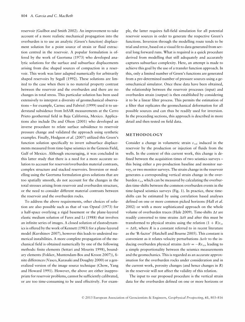
Figure 1 Illustration of the overburden strain field arising from aconcentrated source of strain in the reservoir. The method seeks toinvert the overburden measurements directly onto their origin.

a volume (i = 1,N) as εzz(xhi,yhi,zhi). The production-inducedvolumetric reservoir strain changes εvol (xrj,yrj) are definedon the top reservoir surface with a grid of unknowns witha preset resolution (j = 1,M cells) to be determined in theprocedure. Finally, whilst the mathematical relation that linksthese two strain fields to each other could be calculated viathe Geertsma formulation or numerically, we choose here totake another approach in its evaluation. By reorganizing bothsets of 2D strain data into column vectors, it is proposed thatthe following equation can be formed:

f ∗ m = d, (1)

where d is the vector of the measured overburden strainchanges as defined above and m a vector representing thereservoir strain changes. In our work m can also be the straincentres for more than one source. The vector f is an unknownfunction capturing the desired geomechanical propagator. Theasterisk represents a 1D convolution operation and as suchequation (1) becomes a well-recognized equation in the linearfilter theory. Indeed, if for a particular m the correspondingoverburden strain d is known, as is the case in numericalsimulation, then a physically consistent, causal filter f can bedetermined by minimizing the known and predicted outputsd with constraints. This leads to the least squares or Wienerfilter estimate of f W (Robinson and Treitel 1967). Havingobtained an estimate of f = f W for a given d and specificm, equation (1) can now be redefined as an inverse problem

when applied to the data. Thus, it is now possible to estimatethe reservoir volumetric strain distribution m’ that might havecaused a given observed overburden strain change dob by con-volving these measurements with the inverse filter f−1

W (this isWiener deconvolution – Gonzalez and Wintz 1983)

〈 f −1〉(xr , yr )

m′ = {f−1w } ∗ dob. (2)

In our work, we propose a three step procedure: firstly severalfWj are estimated by using the overburden strain changes calcu-lated by numerical simulation of the displacement fields froma number (j = 1, P) of strategically located reference sourcesof the reservoir strain. The overburden strain correspondingto each source is obtained by running a geomechanical sim-ulation. Secondly, for the Wiener filter functions correspond-ing to each source, the corresponding inverse function f −1

Wjis

computed. Finally, a combination of these inverse functionsfor each reference source-overburden strain pair is calculated,which permits the inversion of an arbitrary observed overbur-den strain field and takes into account lateral variability. Thedesired combination of inverse functions varies according toeach cell location (xr,yr) in the reservoir and is calculated bythe weighting wj (j = 1, P) of the reference source contribu-tions according to the nearness of the desired point to eachreference location. Thus:

⟨f −1W

⟩(xr , yr ) =

P∑

j=1

w j (xr , yr ){

f −1Wj

}, (3)

where w j (xr , yr ) = e−β/Rj and β is a preset constant and Rj thedistance from the cell of interest to each reference source j. Inpractice β is determined by trial and error and is adjusted un-til a smooth and stable solution can be determined. Thus, thereservoir strain corresponding to a particular measured over-burden strain is determined by combining the contributionsfor each cell in the reservoir grid and then applying the averageinverse function. The computation moves through the reser-voir cell by cell and continues until each grid contribution hasbeen evaluated. Essentially this produces a Green’s functionsolution that adapts to each location over the reservoir.

Given a reliable model of the overburden and reservoir thatcaptures the structural complexity and material contrasts,then each of the computations above capture the variabil-ity that is missing in the analytic solution approach. Withthe availability of additional numerically computed overbur-den strains from individual sources distributed widely andmore densely over the reservoir, an increasing amount of in-formation on the lateral variations may be captured. Clearly,



however there is a trade-off between the number of forwardcalculations performed by a time-consuming simulation andthe supply of sufficient information for an accurate inversion.

DATA APPLICA T I ON

Background to the field data

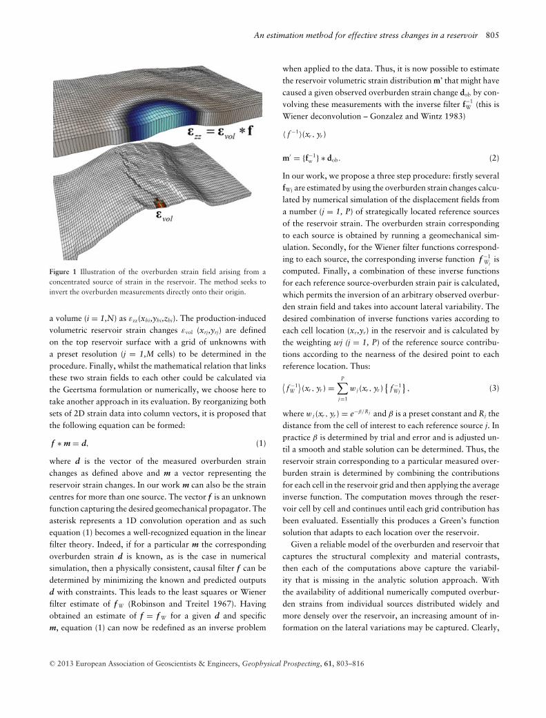
The data for this study are from the South Arne field in theDanish North Sea (Fig. 2). This is a chalk field of Maas-trichtian and Danian age, with the reservoir structure beingan elongated double-dipping anticline with a long axis ori-ented NW-SE and a graben-like structure on the crest (Cipolla,Hansen and Ginty 2007, Fig. 3). There are two high-porosity,low-permeability reservoir units corresponding to the Ekofiskand the underlying, more productive Tor formations (Fig. 4).These formations are separated by a low-porosity low- perme-ability interval at the bottom of the Ekofisk formation knownas the tight zone, lying at a subsea depth of approximately2900 m (2600 ms). Top Ekofisk is picked on a trough on theseismics and Top Tor on a peak, whilst the base of Tor is notclearly defined on the seismics (Fig. 5). The combined thick-nesses of the Ekofisk and Tor reservoirs vary from 10–150 mbut these are highly variable and lie unconformably betweenthick shale layers. The best quality rock lies on the north flankin the Tor formation with porosities ranging from 20–45%.Matrix permeability ranges from 0.1–10 mD, with fracturesand faults providing the main contribution. The reservoir isthinner towards the crest of the structure and also thins down

Figure 2 The geographical location of the South Arne field, relativeto the Danish and Dutch mainland.

Figure 3 Structural map of the South Arne field together with thecross-section A-B corresponding to the vertical sections of Figs 4 and5.

towards the unconformity southwards along the crest. Asthe chalk sequence thickens down dip, the porosity and per-meability decrease considerably (MacKertich and Goulding1999). As a consequence, pressure support from the aquifer isthought to be negligible since the oil water contact lies on thedistal part of the structure where the permeability is lowest.

The field came on stream in 1999 from horizontal wellsdrilled parallel to the natural fracture orientation and the axisof the reservoir (Fig. 6). Wells are drilled in the upper thirdof Tor, although some degree (20–30%) of communicationis expected between the Ekofisk and Tor formations due thevertical orientation of the hydraulic fractures and the faultsystems. All wells were completed with multiple induced ver-tical hydraulic fractures due to the low permeability of thechalk. The production data indicate a complex reservoir withheterogeneous porosity and permeability distribution. A fieldinjector programme started in 2000 and with weak aquifersupport and a reasonably flat structure, the injectors weredrilled parallel to interleaved producers (Wesnaes, Habso andGinty 2002). The horizontal well trajectories thus form a dis-tinctive parallel railroad track pattern oriented along the min-imum horizontal stress. Although most of the drive energyfor hydrocarbon production comes from this water injection,it is estimated that on the crest of the reservoir, up to 20%



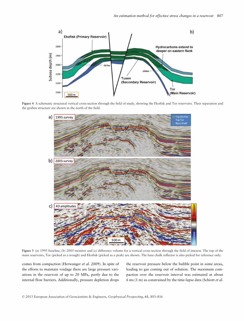
Figure 4 A schematic structural vertical cross-section through the field of study, showing the Ekofisk and Tor reservoirs. Their separation andthe graben structure are shown in the north of the field.

Figure 5 (a) 1995 baseline, (b) 2005 monitor and (c) difference volume for a vertical cross-section through the field of interest. The top of themain reservoirs, Tor (picked as a trough) and Ekofisk (picked as a peak) are shown. The base chalk reflector is also picked for reference only.

comes from compaction (Herwanger et al. 2009). In spite ofthe efforts to maintain voidage there are large pressure vari-ations in the reservoir of up to 20 MPa, partly due to theinternal flow barriers. Additionally, pressure depletion drops

the reservoir pressure below the bubble point in some areas,leading to gas coming out of solution. The maximum com-paction over the reservoir interval was estimated at about6 ms (1 m) as constrained by the time-lapse data (Schiott et al.



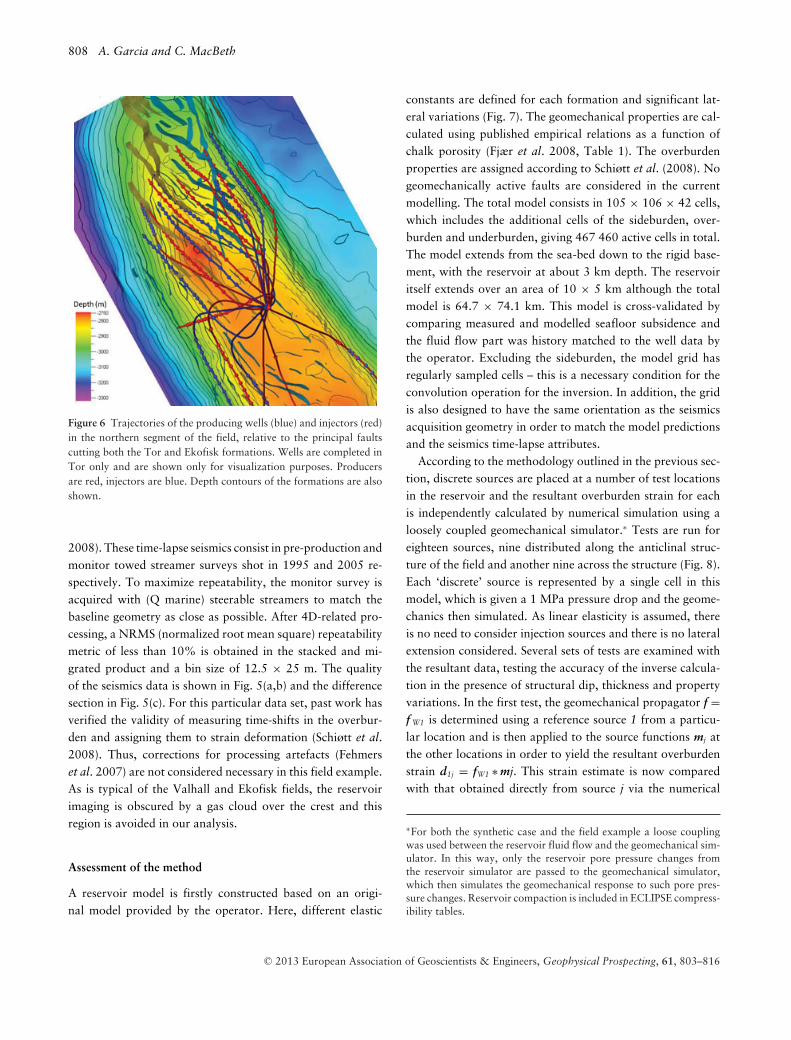
Figure 6 Trajectories of the producing wells (blue) and injectors (red)in the northern segment of the field, relative to the principal faultscutting both the Tor and Ekofisk formations. Wells are completed inTor only and are shown only for visualization purposes. Producersare red, injectors are blue. Depth contours of the formations are alsoshown.

2008). These time-lapse seismics consist in pre-production andmonitor towed streamer surveys shot in 1995 and 2005 re-spectively. To maximize repeatability, the monitor survey isacquired with (Q marine) steerable streamers to match thebaseline geometry as close as possible. After 4D-related pro-cessing, a NRMS (normalized root mean square) repeatabilitymetric of less than 10% is obtained in the stacked and mi-grated product and a bin size of 12.5 × 25 m. The qualityof the seismics data is shown in Fig. 5(a,b) and the differencesection in Fig. 5(c). For this particular data set, past work hasverified the validity of measuring time-shifts in the overbur-den and assigning them to strain deformation (Schiøtt et al.2008). Thus, corrections for processing artefacts (Fehmerset al. 2007) are not considered necessary in this field example.As is typical of the Valhall and Ekofisk fields, the reservoirimaging is obscured by a gas cloud over the crest and thisregion is avoided in our analysis.

Assessment of the method

A reservoir model is firstly constructed based on an origi-nal model provided by the operator. Here, different elastic

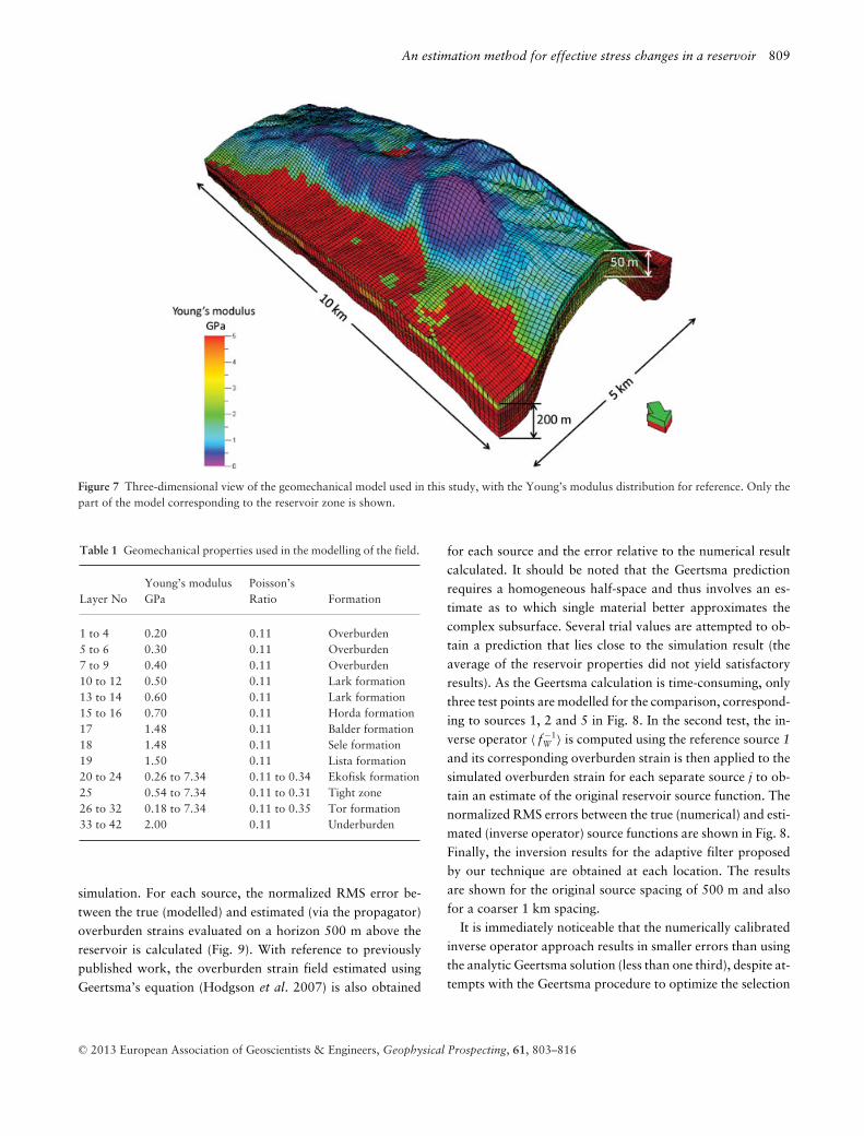
constants are defined for each formation and significant lat-eral variations (Fig. 7). The geomechanical properties are cal-culated using published empirical relations as a function ofchalk porosity (Fjær et al. 2008, Table 1). The overburdenproperties are assigned according to Schiøtt et al. (2008). Nogeomechanically active faults are considered in the currentmodelling. The total model consists in 105 × 106 × 42 cells,which includes the additional cells of the sideburden, over-burden and underburden, giving 467 460 active cells in total.The model extends from the sea-bed down to the rigid base-ment, with the reservoir at about 3 km depth. The reservoiritself extends over an area of 10 × 5 km although the totalmodel is 64.7 × 74.1 km. This model is cross-validated bycomparing measured and modelled seafloor subsidence andthe fluid flow part was history matched to the well data bythe operator. Excluding the sideburden, the model grid hasregularly sampled cells – this is a necessary condition for theconvolution operation for the inversion. In addition, the gridis also designed to have the same orientation as the seismicsacquisition geometry in order to match the model predictionsand the seismics time-lapse attributes.

According to the methodology outlined in the previous sec-tion, discrete sources are placed at a number of test locationsin the reservoir and the resultant overburden strain for eachis independently calculated by numerical simulation using aloosely coupled geomechanical simulator.∗ Tests are run foreighteen sources, nine distributed along the anticlinal struc-ture of the field and another nine across the structure (Fig. 8).Each ‘discrete’ source is represented by a single cell in thismodel, which is given a 1 MPa pressure drop and the geome-chanics then simulated. As linear elasticity is assumed, thereis no need to consider injection sources and there is no lateralextension considered. Several sets of tests are examined withthe resultant data, testing the accuracy of the inverse calcula-tion in the presence of structural dip, thickness and propertyvariations. In the first test, the geomechanical propagator f =f W1 is determined using a reference source 1 from a particu-lar location and is then applied to the source functions mj atthe other locations in order to yield the resultant overburdenstrain d1j = fW1 ∗ mj. This strain estimate is now comparedwith that obtained directly from source j via the numerical

∗For both the synthetic case and the field example a loose couplingwas used between the reservoir fluid flow and the geomechanical sim-ulator. In this way, only the reservoir pore pressure changes fromthe reservoir simulator are passed to the geomechanical simulator,which then simulates the geomechanical response to such pore pres-sure changes. Reservoir compaction is included in ECLIPSE compress-ibility tables.



Figure 7 Three-dimensional view of the geomechanical model used in this study, with the Young’s modulus distribution for reference. Only thepart of the model corresponding to the reservoir zone is shown.

Table 1 Geomechanical properties used in the modelling of the field.

Young’s modulus Poisson’sLayer No GPa Ratio Formation

1 to 4 0.20 0.11 Overburden5 to 6 0.30 0.11 Overburden7 to 9 0.40 0.11 Overburden10 to 12 0.50 0.11 Lark formation13 to 14 0.60 0.11 Lark formation15 to 16 0.70 0.11 Horda formation17 1.48 0.11 Balder formation18 1.48 0.11 Sele formation19 1.50 0.11 Lista formation20 to 24 0.26 to 7.34 0.11 to 0.34 Ekofisk formation25 0.54 to 7.34 0.11 to 0.31 Tight zone26 to 32 0.18 to 7.34 0.11 to 0.35 Tor formation33 to 42 2.00 0.11 Underburden

simulation. For each source, the normalized RMS error be-tween the true (modelled) and estimated (via the propagator)overburden strains evaluated on a horizon 500 m above thereservoir is calculated (Fig. 9). With reference to previouslypublished work, the overburden strain field estimated usingGeertsma’s equation (Hodgson et al. 2007) is also obtained

for each source and the error relative to the numerical resultcalculated. It should be noted that the Geertsma predictionrequires a homogeneous half-space and thus involves an es-timate as to which single material better approximates thecomplex subsurface. Several trial values are attempted to ob-tain a prediction that lies close to the simulation result (theaverage of the reservoir properties did not yield satisfactoryresults). As the Geertsma calculation is time-consuming, onlythree test points are modelled for the comparison, correspond-ing to sources 1, 2 and 5 in Fig. 8. In the second test, the in-verse operator 〈 f −1

W 〉 is computed using the reference source 1

and its corresponding overburden strain is then applied to thesimulated overburden strain for each separate source j to ob-tain an estimate of the original reservoir source function. Thenormalized RMS errors between the true (numerical) and esti-mated (inverse operator) source functions are shown in Fig. 8.Finally, the inversion results for the adaptive filter proposedby our technique are obtained at each location. The resultsare shown for the original source spacing of 500 m and alsofor a coarser 1 km spacing.

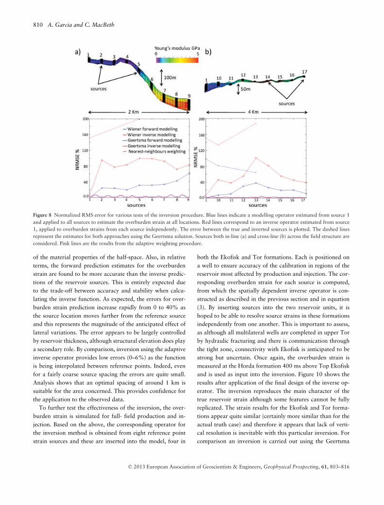
It is immediately noticeable that the numerically calibratedinverse operator approach results in smaller errors than usingthe analytic Geertsma solution (less than one third), despite at-tempts with the Geertsma procedure to optimize the selection



Figure 8 Normalized RMS error for various tests of the inversion procedure. Blue lines indicate a modelling operator estimated from source 1and applied to all sources to estimate the overburden strain at all locations. Red lines correspond to an inverse operator estimated from source1, applied to overburden strains from each source independently. The error between the true and inverted sources is plotted. The dashed linesrepresent the estimates for both approaches using the Geertsma solution. Sources both in-line (a) and cross-line (b) across the field structure areconsidered. Pink lines are the results from the adaptive weighting procedure.

of the material properties of the half-space. Also, in relativeterms, the forward prediction estimates for the overburdenstrain are found to be more accurate than the inverse predic-tions of the reservoir sources. This is entirely expected dueto the trade-off between accuracy and stability when calcu-lating the inverse function. As expected, the errors for over-burden strain prediction increase rapidly from 0 to 40% asthe source location moves further from the reference sourceand this represents the magnitude of the anticipated effect oflateral variations. The error appears to be largely controlledby reservoir thickness, although structural elevation does playa secondary role. By comparison, inversion using the adaptiveinverse operator provides low errors (0–6%) as the functionis being interpolated between reference points. Indeed, evenfor a fairly coarse source spacing the errors are quite small.Analysis shows that an optimal spacing of around 1 km issuitable for the area concerned. This provides confidence forthe application to the observed data.

To further test the effectiveness of the inversion, the over-burden strain is simulated for full- field production and in-jection. Based on the above, the corresponding operator forthe inversion method is obtained from eight reference pointstrain sources and these are inserted into the model, four in

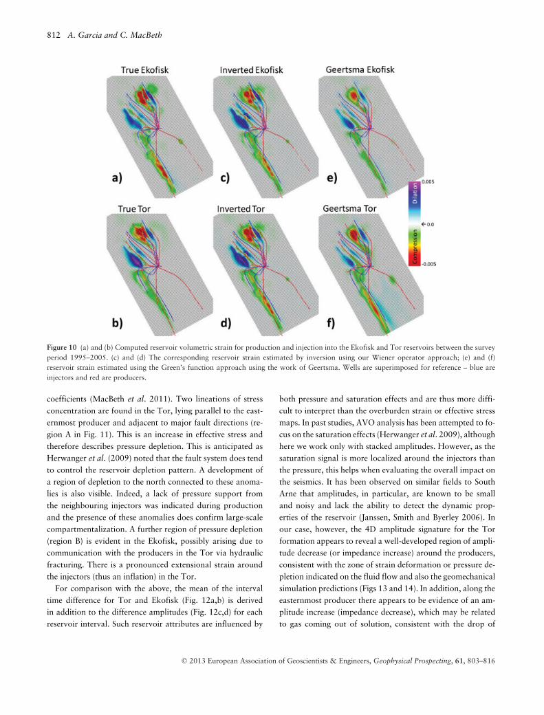
both the Ekofisk and Tor formations. Each is positioned ona well to ensure accuracy of the calibration in regions of thereservoir most affected by production and injection. The cor-responding overburden strain for each source is computed,from which the spatially dependent inverse operator is con-structed as described in the previous section and in equation(3). By inserting sources into the two reservoir units, it ishoped to be able to resolve source strains in these formationsindependently from one another. This is important to assess,as although all multilateral wells are completed in upper Torby hydraulic fracturing and there is communication throughthe tight zone, connectivity with Ekofisk is anticipated to bestrong but uncertain. Once again, the overburden strain ismeasured at the Horda formation 400 ms above Top Ekofiskand is used as input into the inversion. Figure 10 shows theresults after application of the final design of the inverse op-erator. The inversion reproduces the main character of thetrue reservoir strain although some features cannot be fullyreplicated. The strain results for the Ekofisk and Tor forma-tions appear quite similar (certainly more similar than for theactual truth case) and therefore it appears that lack of verti-cal resolution is inevitable with this particular inversion. Forcomparison an inversion is carried out using the Geertsma



Figure 9 A selection of the results from the tests of the transfer function approach. (a) Estimates of overburden strain from a transfer functionestimated using the numerical results from source 1 alone and re-applied to source 15. (b) Estimates of the source obtained by inversion of theoverburden strain using the operator estimated from source 1 results applied to the overburden strain generated by source 15. The Geertsmasolutions are also shown for reference.

procedure following the work of Hodgson et al. (2007)(Fig. 10e,f). These results are observed to be smoother hori-zontally but to have a similar location, distribution and po-larity for the strain anomalies.

Results of field data analysis

The above approach is now applied to the observed time-lapseseismics data. Time-lapse time-shifts of the order of a few mil-liseconds are obtained using 3D warp analysis of the seismicsdata. These time-shifts are calculated again using the methodof Hale (2009), which is applied over the volume of tracesfor the baseline and monitor surveys between 1600–3400 ms,which includes the overburden and the reservoir. This pro-duces spatially smoothed time-shift estimates at every timesample in the seismics within that range. Lateral shifts arealso computed by the algorithm but not used further in ourwork. The accuracy of the final warp field is judged by apply-ing it directly to the monitor survey, from which the degreeof match with the baseline seismics can be directly compared.Using the results of the previous section as a guide, these time-shifts are converted to time strains as above and the average in

a window between the top and base of the Horda formationis taken as input into the inversion. Next, the inverse opera-tor is determined using simulations of the average time straincomputed from the geomechanical model described in the pre-vious section. Following the synthetic study, eight sources areemployed, four for each reservoir formation and these aredistributed with the same pattern as in the synthetic study.

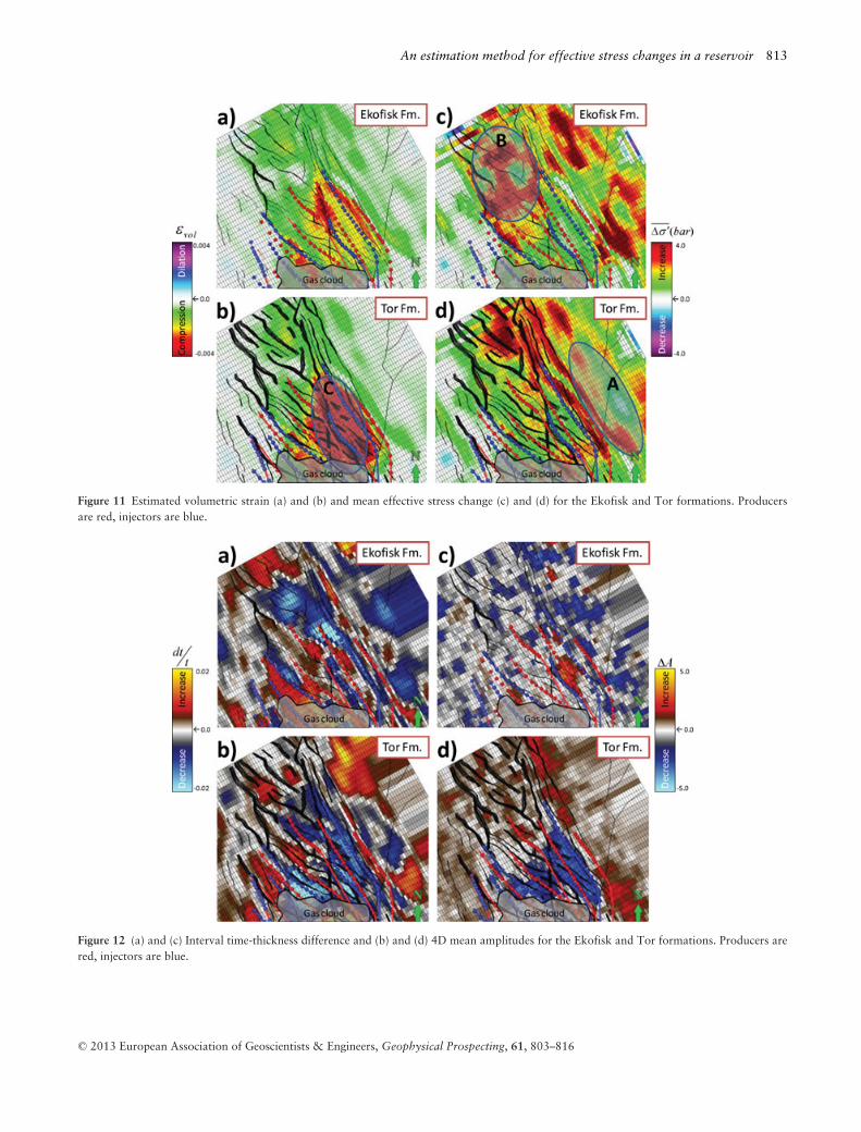
The final results of applying the operator to invert for thevolumetric strain in the reservoir are shown in Fig. 11(a,b)for the Ekofisk and Tor formations respectively. To furtherinterpret these results, the strain maps εvol are converted intomean effective stress �σ (Fig. 11c,d). This is achieved by uti-lizing the simple linear relationship �σ = κεvol where κ is theporosity-dependent isotropic bulk modulus calculated accord-ing to Fjær et al. (2008). This transformation is important,as high porosity can lead to high-strain rates but low stress(and hence pressure) changes and vice-versa and can mis-lead the reservoir interpretation. Conversion to effective stresschanges facilitates interpretation in terms of the relative reser-voir pressure change. Thus, upward pressure change leads toa decrease of effective stress and vice versa, although the pre-cise relationship depends on the effective stress and arching



Figure 10 (a) and (b) Computed reservoir volumetric strain for production and injection into the Ekofisk and Tor reservoirs between the surveyperiod 1995–2005. (c) and (d) The corresponding reservoir strain estimated by inversion using our Wiener operator approach; (e) and (f)reservoir strain estimated using the Green’s function approach using the work of Geertsma. Wells are superimposed for reference – blue areinjectors and red are producers.

coefficients (MacBeth et al. 2011). Two lineations of stressconcentration are found in the Tor, lying parallel to the east-ernmost producer and adjacent to major fault directions (re-gion A in Fig. 11). This is an increase in effective stress andtherefore describes pressure depletion. This is anticipated asHerwanger et al. (2009) noted that the fault system does tendto control the reservoir depletion pattern. A development ofa region of depletion to the north connected to these anoma-lies is also visible. Indeed, a lack of pressure support fromthe neighbouring injectors was indicated during productionand the presence of these anomalies does confirm large-scalecompartmentalization. A further region of pressure depletion(region B) is evident in the Ekofisk, possibly arising due tocommunication with the producers in the Tor via hydraulicfracturing. There is a pronounced extensional strain aroundthe injectors (thus an inflation) in the Tor.

For comparison with the above, the mean of the intervaltime difference for Tor and Ekofisk (Fig. 12a,b) is derivedin addition to the difference amplitudes (Fig. 12c,d) for eachreservoir interval. Such reservoir attributes are influenced by

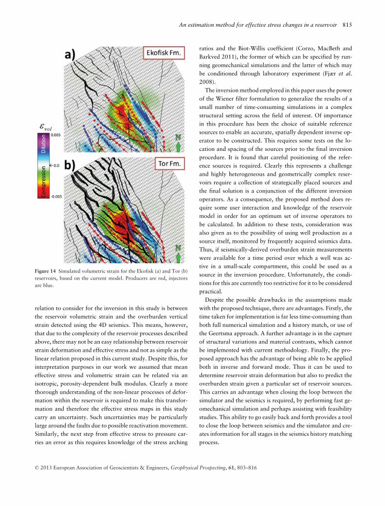
both pressure and saturation effects and are thus more diffi-cult to interpret than the overburden strain or effective stressmaps. In past studies, AVO analysis has been attempted to fo-cus on the saturation effects (Herwanger et al. 2009), althoughhere we work only with stacked amplitudes. However, as thesaturation signal is more localized around the injectors thanthe pressure, this helps when evaluating the overall impact onthe seismics. It has been observed on similar fields to SouthArne that amplitudes, in particular, are known to be smalland noisy and lack the ability to detect the dynamic prop-erties of the reservoir (Janssen, Smith and Byerley 2006). Inour case, however, the 4D amplitude signature for the Torformation appears to reveal a well-developed region of ampli-tude decrease (or impedance increase) around the producers,consistent with the zone of strain deformation or pressure de-pletion indicated on the fluid flow and also the geomechanicalsimulation predictions (Figs 13 and 14). In addition, along theeasternmost producer there appears to be evidence of an am-plitude increase (impedance decrease), which may be relatedto gas coming out of solution, consistent with the drop of



Figure 11 Estimated volumetric strain (a) and (b) and mean effective stress change (c) and (d) for the Ekofisk and Tor formations. Producersare red, injectors are blue.

Figure 12 (a) and (c) Interval time-thickness difference and (b) and (d) 4D mean amplitudes for the Ekofisk and Tor formations. Producers arered, injectors are blue.



Figure 13 Predicted water saturation (a) and (b) and pressure (c) and (d) changes for the Ekofisk and Tor formations based on the current flowsimulation model. Note that water saturations cannot be detected from our current technique and thus cannot validate this model. Pressurechanges should however be matched to our results. Producers are red, injectors are blue.

pressure. In the Ekofisk difference amplitudes there is a small,localized zone of impedance decrease associated with an in-jector that is known to have partially penetrated the Ekofiskat that location. To the east of the area, there may be somedevelopment of an impedance decrease, although it is difficultto attribute a precise cause. The interval times show an in-crease at the westernmost injectors, associated with a pressureup, whilst the second set of injectors to the east show a de-crease that may be associated with the overall pressure downarea around these producers. The inversion results identify thestudy area as heterogeneous, with three major pressure com-partments and moderate pressure connection between the Torand Ekofisk formations.

DISCUSS ION A N D C ON C LUSI ON S

There are a myriad of techniques where surface measured datacan be inverted into subsurface properties, such as gravimetricand magnetic surveys, tiltmeter data and satellite interferom-etry. To add to these, 4D seismics data have recently alsobeen shown to provide a valuable source of data on the over-burden strain deformation due to reservoir production andrecovery. Furthermore, it has been shown in this and other

studies, that these data can be inverted to yield informationon the reservoir’s effective stress changes and hence an infer-ence of reservoir pressure distributions can be made. This isuseful information to help guide dynamic reservoir manage-ment. However, it is important to understand the assumptionsinherent in this procedure and how these relate to the choicesmade for the inversion in this current work.

The first set of assumptions for our method relates to thechoice of effective stress or pressure as the final inversionproduct. Reservoirs seldomly behave in a linear elastic fashion(Audet and Fowler 1992), such that highly depleted reservoirswill display different elastic behaviour than anticipated byinitial conditions – some may deform plastically, others mayexperience pore collapse, or chalk reservoirs may undergo wa-ter weakening. Thus, the most appropriate way to representthis range of processes is to treat the reservoir as a source ofstrain only. The overburden materials, by comparison, do notexperience any significant changes in their constituency andonly react to net reservoir deformation and they can safelybe considered as essentially elastic (Vasco and Ferretti 2005).Indeed, regardless of how the reservoir deforms, the inducedoverburden displacements can usually always be consideredelastic. A consequence of this is that the most appropriate



Figure 14 Simulated volumetric strain for the Ekofisk (a) and Tor (b)reservoirs, based on the current model. Producers are red, injectorsare blue.

relation to consider for the inversion in this study is betweenthe reservoir volumetric strain and the overburden verticalstrain detected using the 4D seismics. This means, however,that due to the complexity of the reservoir processes describedabove, there may not be an easy relationship between reservoirstrain deformation and effective stress and not as simple as thelinear relation proposed in this current study. Despite this, forinterpretation purposes in our work we assumed that meaneffective stress and volumetric strain can be related via anisotropic, porosity-dependent bulk modulus. Clearly a morethorough understanding of the non-linear processes of defor-mation within the reservoir is required to make this transfor-mation and therefore the effective stress maps in this studycarry an uncertainty. Such uncertainties may be particularlylarge around the faults due to possible reactivation movement.Similarly, the next step from effective stress to pressure car-ries an error as this requires knowledge of the stress arching

ratios and the Biot-Willis coefficient (Corzo, MacBeth andBarkved 2011), the former of which can be specified by run-ning geomechanical simulations and the latter of which maybe conditioned through laboratory experiment (Fjær et al.2008).

The inversion method employed in this paper uses the powerof the Wiener filter formulation to generalize the results of asmall number of time-consuming simulations in a complexstructural setting across the field of interest. Of importancein this procedure has been the choice of suitable referencesources to enable an accurate, spatially dependent inverse op-erator to be constructed. This requires some tests on the lo-cation and spacing of the sources prior to the final inversionprocedure. It is found that careful positioning of the refer-ence sources is required. Clearly this represents a challengeand highly heterogeneous and geometrically complex reser-voirs require a collection of strategically placed sources andthe final solution is a conjunction of the different inversionoperators. As a consequence, the proposed method does re-quire some user interaction and knowledge of the reservoirmodel in order for an optimum set of inverse operators tobe calculated. In addition to these tests, consideration wasalso given as to the possibility of using well production as asource itself, monitored by frequently acquired seismics data.Thus, if seismically-derived overburden strain measurementswere available for a time period over which a well was ac-tive in a small-scale compartment, this could be used as asource in the inversion procedure. Unfortunately, the condi-tions for this are currently too restrictive for it to be consideredpractical.

Despite the possible drawbacks in the assumptions madewith the proposed technique, there are advantages. Firstly, thetime taken for implementation is far less time-consuming thanboth full numerical simulation and a history match, or use ofthe Geertsma approach. A further advantage is in the captureof structural variations and material contrasts, which cannotbe implemented with current methodology. Finally, the pro-posed approach has the advantage of being able to be appliedboth in inverse and forward mode. Thus it can be used todetermine reservoir strain deformation but also to predict theoverburden strain given a particular set of reservoir sources.This carries an advantage when closing the loop between thesimulator and the seismics is required, by performing fast ge-omechanical simulation and perhaps assisting with feasibilitystudies. This ability to go easily back and forth provides a toolto close the loop between seismics and the simulator and cre-ates information for all stages in the seismics history matchingprocess.



ACKNOWLEDG E ME N T S

We thank the sponsors of the Edinburgh Time Lapse Project,Phases III and IV (BG, BP, Chevron, ConocoPhillips, EnCana,ENI, ExxonMobil, Hess, Ikon Science, Landmark, Maersk,Marathon, Norsar, Rock Solid Images, Petrobras, Shell, Sta-toil, Total and Woodside) for supporting this research. Wethank Schlumberger-Geoquest for the use of their Petrel,Eclipse and Visage software. Thanks also to Ole Vejbæk andChristian Schiøtt for helpful discussions.

REFERENCES

Audet D. and Fowler A. 1992. A mathematical model for com-paction in sedimentary basins. Geophysics Journal International110, 557–590.

Carnec C. and Fabriol H. 1999. Monitoring and modeling land sub-sidence at the Cerro Prieto geothermal field, Baja California, Mex-ico, using SAR interferometry. Geophysical Research Letters 26,1211–1214.

Chow Y.L., Yang J.J. and Howard G.E. 1991. Complex Im-ages for Electrostatic Field Computation in Multilayered Media.IEEE Transactions on Microwave Theory and Techniques 39,1120–1125.

Cipolla C.L., Hansen K.K. and Ginty W.R. 2007. Fracture TreatmentDesign and Execution in Low-Porosity Chalk Reservoirs. SPE Pro-duction and Operations 22(1), 94–106.

Corzo M., MacBeth C. and Barkved O. 2011. Estimation of pressurechanges in a compacting reservoir from time-lapse seismic data.Geophysical Prospecting, doi: 10.1111/1365-2478.12037.

Du J. and Olson J.E. 2001. A poroelastic reservoir model for predict-ing subsidence and mapping subsurface pressure fronts. Journal ofPetroleum Science and Engineering 30, 181–197.

Fares N. and Li V. 1988. General image method in a plane-layeredelastostatic medium. Journal of Applied Mechanics 55, 781–785.

Fehmers G.C., Hunt K., Brain J.P., Bergler S., Kaestner U., SchutjensP.M. and Burrell R.V. 2007. Curlew D – Pushing the boundariesof 4D depletion signal in a gas condensate field, UK Central NorthSea. Presented at the Annual EAGE Conference, P074.

Fjær E., Holt R., Raaen A., Risnes R. and Horsrud P. 2008. PetroleumRelated Rock Mechanics. (2nd Edition). Elsevier Academic Press.

Fokker P.A., Muntendam-Bos A.G. and Kroon I.C. 2007. InverseModelling of Surface Subsidence to Better Understand the Earth’sSubsurface. First Break 25, 101–105.

Geertsma J. 1973. A Basic Theory of Subsidence due to ReservoirCompaction: The Homogeneous Case. Verhandelingen Kon. Ned.Geol. Mijnbouwk. Gen. 28, 43–62.

Gonzalez R.C. and Wintz P. 1983. Digital Image Processing. Addison-Wesley Publishing Company.

Guilbot J. and Smith B. 2002. 4D constrained depth conversion forreservoir compaction estimation: Application to Ekofisk Field. TheLeading Edge 21, 302–308.

Hale D. 2009. A method for estimating apparent displacement vectorsfrom time-lapse seismic images. Geophysics 74(5), 99–107.

Hall S.A., MacBeth C., Barkved O.I. and Wild P. 2002. Time-lapse seismic monitoring of compaction and subsidence at Valhallthrough crossmatching and interpreted warping of 3D streamerand OBC data. SEG International Exposition and 72nd AnnualMeeting. Salt Lake City, Utah.

Hatchell P. and Bourne S. 2005. Rocks under strain: Strain-inducedtime-lapse time shifts are observed for depleting reservoirs. TheLeading Edge 24, 1222–1225.

Herwanger J.V., Schiøtt C.R., Frederiksen R., Vejbæk O.V., WoldR. and Hansen H.J. 2009. Applying time-lapse seismic methodsto reservoir management and field development planning at SouthArne, Danish North Sea. In: Petroleum Geology: From MatureBasins to New Frontiers – Proceedings of the 7th Petroleum Ge-ology Conference, (ed. B. &. Vining), pp. 523–535. London: Geo-logical Society, London.

Hodgson N., MacBeth C., Duranti L., Rickett J. and Nihei K. 2007.Inverting for reservoir pressure change using time-lapse time strain:Application to Genesis Field, Gulf of Mexico. The Leading Edge26, 649–652.

Janssen A.L., Smith B.A. and Byerley G.W. 2006. Measuring velocitysensitivity to production-induced strain at the Ekofsk Field usingtime-lapse time-shifts and compaction logs. SEG Annual Interna-tional Meeting, pp. 3200–3203. New Orleans.

Kennett B. 1983. SeismicWave Propagation in Stratified Media. Cam-bridge University Press.

Kuvshinov B.N. 2007. Reflectivity Method for Geomechanical Equi-libria. Geophysical Journal International 170, 567–579.

MacBeth C., HajNasser Y., Stephen K. and Gardiner A. 2011. Explor-ing the effect of meso-scale shale beds on a reservoir’s overall stresssensitivity to seismic waves. Geophysical Prospecting 59, 90–110.

Mackertich D.S. and Goulding D.R. 1999. Exploration and appraisalof the South Arne Field, Danish North Sea. Petroleum GeologyConference series, pp. 959–974. London.

van Opstal G. 1973. The Effect of Base-Rock Rigidity on Subsidencedue to Reservoir Compaction. Proceedings of the Third Congressof the International Society of Rock Mechanics.

Robinson E.A. and Treitel S. 1967. Principles Of Digital Wiener Fil-tering. Geophysical Prospecting 15, 311–332.

Schiøtt C.R., Bertrand-Biran V., Hanse H.J., Koutsabeloulis N. andWesteng K. 2008. Time-lapse inversion and geomechanical mod-elling of the South Arne field. First Break 26, 85–91.

Segall P. 1992. Induced stresses due to fluid extraction from axisym-metric reservoirs. Pure and Applied Geophysics, 535–560.

Settari A. and Mourits F. 1998. A coupled reservoir and geomechan-ical simulation system. SPE Journal, 219–226.

Vasco D.W. and Ferretti A. 2005. On the use of quasi-static deforma-tion to understand reservoir fluid flow. Geophysics 70, 013–027.

Vasco D.W., Karasaki K. and Doughty C. 2000. Using surface defor-mation to image reservoir dynamics. Geophysics 65, 132–147.

Wesnæs K., Hasbo K. and Ginty W.R. 2002. Hydraulic FractureSpacing in Horizontal Chalk Producers: The South Arne Field. SPEWestern Regional/AAPG Pacific Section Joint Meeting, Anchorage,Alaska SPE 76722.


an estimation method for effective stress changes in ... - hw an estimation method for effective...

Documents