an evaluation of applying ensemble data assimilation to · pdf filewachowicz et al. p.1 an...

Wachowicz et al. p.1

An Evaluation of Applying Ensemble Data Assimilation to an Antarctic Mesoscale Model

Lori Wachowicz1,2, Steven Cavallo3, and Dave Parsons3

1National Weather Center Research Experiences for Undergraduates Program, Norman Oklahoma and

2Michigan State University, East Lansing, Michigan

3School of Meteorology, University of Oklahoma, Norman, Oklahoma

ABSTRACT Knowledge of Antarctic weather and climate processes relies heavily on models due to the lack of

observations over the continent. The Antarctic Mesoscale Prediction System (AMPS) is a numerical model capable of resolving finer-scale weather phenomena. The Antarctic’s unique geography, with a large ocean surrounding a circular continent containing complex terrain makes fine-scale processes potentially very important features in poleward moisture transport and the mass balance of Antarctica’s ice sheets. AMPS currently uses the 3DVAR method to produce atmospheric analyses (AMPS-3DVAR), which may not be well-suited for data-sparse regions like the Antarctic and Southern Ocean. To optimally account for flow-dependence and data sparseness unique to this region, we test the application of an ensemble adjustment Kalman Filter (EAKF) within the framework of the Data Assimilation Research Testbed (DART) and AMPS model (A-DART). We test the hypothesis that the application of A-DART improves the AMPS-3DVAR estimate of the atmosphere. We perform a test using a one-month period from 21 September - 21 October 2010 and find comparable results to both AMPS-3DVAR and GFS. In particular, we find a strong cold model bias near the surface and a warm model bias at upper-levels. Investigation of the surface bias reveals strongly biased land-surface observations while the warm bias at upper-levels is likely a circulation bias from the model warming too rapidly aloft over the continent. Increasing quality control of surface observations and assimilating polar-orbiting satellite data are expected to alleviate these issues in future tests.

.1. INTRODUCTION The effect of Antarctic processes on the rest of the world with impending climate change has been a cause for concern as about 90 percent of Earth’s fresh water (Mayewski et al. 2009) is contained in Antarctica’s massive ice sheets. The Antarctic Peninsula, along with a few other areas over the continent have experienced temperature increases (Turner et al. 2005), heightening concerns with regard to the fate of the ice sheets. This has motivated the scientific community to better understand the impacts of Antarctic processes on the rest of the world, as the melting of the ice sheet will result in substantially higher sea levels. Knowledge of the factors that affect the mass balance of the ice sheet will aid in the prediction of

1 Corresponding author address: Lori Wachowicz, National Weather Center Research Experiences for Undergraduates Program, Center for Analysis and Prediction of Storms, The University of Oklahoma, National Weather Center, 120 David L. Boren Blvd, Suite 2500, Norman, OK 73072, [email protected].

future climate change events (Mayewski et al. 2009). Unlike the Arctic, there are less people living in and around Antarctica, making the need for observations less of a necessity. However, the lack of observations severely impacts our understanding of Antarctic weather and climate. Furthermore, these few observations are not evenly dispersed around the continent (Jung et al. 2013). Most observations of Antarctica are obtained through automated weather stations (AWS), radiosondes, satellite winds, and marine observations from passing ships. To aid in the forecasting for scientific research flights into the Antarctic, the Antarctic Mesoscale Prediction System (AMPS) model was developed by the National Center for Atmospheric Research (NCAR). It is currently the only routinely-run mesoscale modeling system, providing valuable insight into mesoscale and synoptic processes occurring in and around Antarctica (Powers et al. 2003). It is important to understand these finer-scale processes in the Antarctic because these processes may be significant factors in the poleward transport of moisture, and thus impact the mass balance of the ice sheet. The AMPS


model uses a three-dimensional variational data assimilation system (3DVAR) (Barker et al. 2004) to initialize model simulations that are performed twice daily. While AMPS has been revolutionary for Antarctic weather prediction, the 3DVAR method has some limitations. The primary limitations are that it does not utilize flow-dependent information, and it does not provide an estimate of the uncertainty in a given analysis state or forecast. On the other hand, models using Ensemble Data Assimilation (EnsDA) generally outperform models using 3DVAR and are better-suited for data-sparse regions (Whitaker et al. 2009). Given these previous findings, it is reasonable to expect that an ensemble approach may lead to improvements in AMPS. In this study, we use an ensemble data assimilation approach to test the hypothesis that an ensemble data assimilation improves the analysis estimates of the Antarctic and Southern Ocean currently provided with AMPS. We perform our test for a month-long period from 21 September – 21 October. This period is motivated by the concurrence of the Concordiasi intensive observation period (IOP)-a joint project between the France and the United States. Gondolas were deployed in upper-atmospheric levels that drifted with the atmospheric circulation. From these gondolas, dropsondes were launched periodically, providing a unique opportunity to collect vertical columns of data over the data-sparse Southern Ocean and Antarctic continent (Rabier et al. 2010). Observations of the vertical atmospheric state from Concordiasi provide an independent source for which our modeling results can be evaluated. The remainder of this paper is as follows. A description of our model and our method used to examine our hypothesis is found in Section 2. Our results are discussed in Section 3,and our conclusion and potential future work is listed in Section 4. 2. Methods We use the ensemble adjustment Kalman Filter (EAKF) (Anderson 2001) implementation within the Data Assimilation Research Testbed (DART) (Anderson et al. 2009) framework using 96 ensemble members, and we subsequently refer to this data assimilation system as “A-DART.” We obtain our initial conditions for our very first model run from the Global Forecasting System (GFS) (EMC 2003) model on 21 September 2010 at 00

UTC and subsequently cycle solely using the AMPS model within the DART framework for our initial conditions for the remainder of the experiment ending on 21 October 2010 at 00 UTC. The A-DART system uses a smaller number of observations (~40,000) compared to AMPS-3DVAR (several million) since AMPS-3DVAR is re-initialized from GFS each iteration utilizing all observations assimilated in the National Centers for Environmental Prediction (NCEP) global data assimilation system. The A-DART model uses a horizontal grid spacing of 45 km with 44 unevenly-spaced vertical levels. A time step of 144 seconds is used, and we output data at a frequency of 6 hours. The various physics schemes incorporated in A-DART include: WRF Single-Moment 5-class (WSM5) microphysics (Hong et al. 2004), Rapid Radiative Transfer Model (RRTM) longwave radiation (Mlawer et al. 1997), Goddard shortwave radiation (Chou and Suarez 1994), Monin-Obukhov surface layer physics(Paulson 1970; Dyer and Hicks 1970; Webb 1970), Noah land surface model (Chen and Dudhia 2001), Mellor-Yamada-Janjic boundary layer scheme (Janjic 1994).

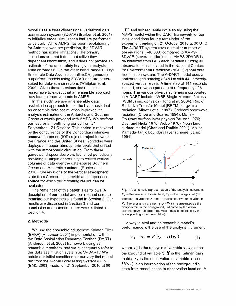
A way to evaluate an ensemble model’s performance is the use of the analysis increment (1)

where is the analysis of variable , is the background of variable , is the Kalman gain matrix, is the observation of variable , and

is an interpolation of the background’s state from model space to observation location. A

Fig. 1 A schematic representation of the analysis increment. is the analysis of variable , is the background (6-h

forecast ) of variable and is the observation of variable . The analysis increment ( - ) is represented as the

analysis minus the background, indicated by the arrow pointing down (colored red). Model bias is indicated by the arrow pointing up (colored blue).


more visual representation is shown in Figure 1. We apply this diagnostic to evaluate the performance of A-DART. For example, (1) quantifies the impact that observations have on short-term AMPS-3DVAR model forecasts at each output time. A smaller analysis increment implies there is a low model bias, since the observations in that case are not substantially changing the model’s background estimate of . Conversely, a large analysis increment implies the model’s estimate of is relatively different than observations, implying that there is a large model bias. Furthermore, in a well-calibrated ensemble where observations are unbiased and the spread

of the ensemble represents the true variance of the state, the analysis increment will remain nearly steady between data assimilation cycles. If observations are unbiased, the analysis increment, is equivalent to the negative of the model bias, (Recall Fig. 1). Therefore, the analysis increment provides a method to diagnose model bias. Knowledge of the model bias can help identify weaknesses in the model so that tests can be performed to further isolate possible deficiencies in the model’s physical parameterizations. The analysis increment of temperature at the first model level for both AMPS-3DVAR and A-DART (Fig. 2) show that A-DART surface temperature has less of a bias than that of AMPS. Note that observations are not evenly dispersed throughout the domain, and in particular, most observations are in lower latitudes (equatorward of

45°S) and are primarily atmospheric motion vectors from geostationary satellites. 3. Results The vertical profile of the ensemble mean model temperature bias with respect to radiosonde temperature and root-mean square error (RMSE) from 45-90°S shows comparable biases between A-DART, AMPS-3DVAR, and GFS (Fig. 3). The RMSE of A-DART is larger than AMPS-3DVAR and GFS, however the patterns are similar with peak RMSEs around 250 hPa and at the surface. A-DART has a substantial negative bias at the surface, much larger in comparison to GFS and AMPS-3DVAR. There is a positive temperature bias at all levels above 400 hPa, which is also present in AMPS and GFS. To understand the reasons for these biases, we next focus our diagnostics where the biases are largest: near the surface (1000 hPa) and aloft (300 hPa). One way to determine whether the A-DART ensemble is representing the spread of the true state is to compute rank histograms. A rank histogram evaluates the probability that a particular observation will fall within an ensemble spread. Ensemble members are separated into “bins” by sorting them by their value. A good ensemble will exhibit a flat, or uniform shape, implying that each ensemble member has an equal probability of matching the observed value. A U-shaped or inverted-U-shaped distribution implies the ensembles have too little spread or too much spread, respectively. A negatively

Fig. 2 The analysis increment of temperature at model level 1 for (left) AMPS and (right) A-DART. Locations of observations are overlaid with the observation types listed in the legend below each panel. Blue (red) shadings represent areas of a negative (positive) analysis increment with a contour interval of 0.1 K.

Fig. 3 Vertical profile of the mean model bias and RMSE with respect to radiosonde temperature. Averages are computed from 21 September to 21 October 2010. Solid (dashed) lines indicate the model bias (RMSE). Blue lines correspond to A-DART, red lines correspond to, AMPS, and black lines correspond to GFS is black.


(positively) skewed pattern indicates a cold (warm) model bias.

a. Surface bias At the surface, land surface temperatures are frequently outside either end of the range of the A-DART ensemble members, resembling a U-shape (Fig. 4). This pattern in the rank histogram is an indication that the spread of the A-DART ensemble is too small. There is also a slight tendency for observations to be slightly colder than the ensemble. Note that radiosonde temperatures around 1000 hPa are warmer than the ensemble mean (Recall Fig. 3), however it is unclear whether the cold land surface temperature observations derive from stations at higher altitudes. These factors imply that the observation error covariances are not representative of the true instrument values. The AWS altimeter observations show a similar pattern as the land surface temperatures in that the values tend to fall outside the range of the ensemble members, though they do not have a prevalent cold bias. Overall, by examining different observations at or near the surface, it is clear that our observations need to be re-calibrated in order to reduce A-DART surface temperature bias.

b. Upper-level bias Given the warm temperature bias aloft (Recall Fig. 3), and the fact that observations are not evenly distributed as a function of latitude, we hypothesize that the model is erroneously warming temperatures aloft over the continent, such that it weakens the net upper-level atmospheric circulation. In the upper levels, there are apparent strong wind biases associated with A-DART, compared to AMPS-3DVAR and GFS. The u-wind component becomes increasingly negative with height (Fig. 5) throughout the entire profile. However, the v-wind component remains strictly positive with height (Fig. 5). The wind bias evident in Figure 5 is primarily with respect to geostationary satellite data in lower latitudes, while the temperature bias from Figure 1 is primarily from radiosonde data over the continent. Together, the vertical bias profiles support the hypothesis that a large-scale circulation bias may be occurring in the upper atmosphere in the A-DART ensembles.

Over the South Pole, we expect to see relatively cold temperatures with respect to lower latitudes, such that there is a low-pressure system aloft over the continent that defines the larger-scale Southern Hemisphere polar vortex. A warm temperature bias suggests that the low pressure over the continent is too weak (Figure 6). In the event the aforementioned is true, we would expect to see a specific pattern when looking at the analysis increments for u- and v-wind components since these observations are located along the periphery of the Southern Hemisphere polar vortex: positive values for u-wind near the top with negative values for u-wind near the bottom and positive values for v-wind on the left with negative values for v-wind on the right (Figure 7). This corresponds to a color pattern shown in the figures as well, with reds on the top and left of the domains, and blues on the bottom and right of the domains. We also see a possible relationship between the satellite wind observations and the strength of the analysis increment, as areas with more observations have a stronger analysis increment than areas with fewer observations which may imply that our satellite data quality is poor.

Fig. 4 Rank histogram of (left) land surface temperature and (right) Automated Weather system altimeter observations within 45-90°

Fig. 5 Vertical profile of model (left) u-wind component and (right) v-wind component bias with respect to radiosonde wind components. The A-DART ensemble is represented by blue, AMPS by red, and GFS by black.


4. Discussion and Conclusion The desire to understand finer-scale processes in the Antarctic has motivated the use of an ensemble data assimilation method (EAKF) over a traditional data assimilation method (3DVAR). The 3DVAR approach tends to be limited in that it does not provide an estimate of uncertainty in a forecast. In previous studies, such as that done by Whitaker et al., (2009), show that ensemble data assimilation generally outperforms 3DVAR. When looking at results for AMPS-3DVAR, Bromwich et al. (2005) explained that AMPS was prone to the Antarctic topography leads to AMPS model bias, especially near coastal surface observation systems. After evaluating biases near the surface with an ensemble approach, these types of results are still prominent, implying that while some of the errors may be fixed, there is still some sort of bias. Bromwich also explains that model forecasts tend to improve with height, which counters the results obtained here with A-DART. While A-DART,

AMPS-3DVAR, and GFS generally perform fairly well with respect to temperature until near the 400 hPa level, all three analyses have a warm temperature bias above 400 hPa. It is likely that surface observations may be the cause of this. After a rigorous examination of the analysis increment and its relationship with model bias, and after examining this warm bias aloft, the possible issues with biased surface observations and too little ensemble spread is possibly contributing to a strong cold model bias near the surface. In turn, it is evident that there is a warm temperature bias aloft in the AMPS model over the Antarctic continent, which leads to a potential large-scale circulation bias. It is important to note that the Southern Hemisphere experiences a reduction in ozone in the Southern Hemisphere polar vortex beginning in August and maximizing in October. This is the case in 2010, with the peak ozone loss occurring around 1 October (de Laat and van Weele, 2011). The AMPS model has a fixed ozone concentration, therefore making it likely that A-DART overestimated the amount of ozone. Since ozone is a strong absorber of solar radiation, this would make it plausible that there was too much shortwave radiative heating aloft, resulting in the warmer temperatures in the polar vortex.

Fig. 6 A diagram illustrating the hypothesized circulation of the large-scale Southern Hemispheric polar vortex and its expected bias on a single upper-atmospheric level. is the

analysis of variable and is the background (6-h

forecast ) of variable . The red (blue) arrows represent the analysis increment (model bias). The text “Red U”, “Blue U”, “Red V”, and “Blue V” highlight the pattern and locations of what we expect to find in the analysis increment as described in the text. For example, “Red U” means that we expect to find a positive analysis increment in the u-component wind toward the top of the figure. The analysis, background, and analysis increments all indicate a clock-wise flow around the South Pole (as indicated by the arrow directions). The model bias (the negative of the analysis increment) is indicated by the smaller arrows pointing in a counter-clockwise direction around the South Pole, indicating that the bias is representing a high-pressure bias over the pole.

Fig. 7 The analysis increments for (left) u- and (right) v-wind components for A-DART at model level xxx (near 300 hPa) with the satellite wind observation locations plotted. Blue (Red) shadings represent areas of a negative (positive) analysis increment with a contour interval of xxx meters per second. The u-wind component (left) analysis increment shows the color red towards the top of the domain with blue towards the bottom, indicating a positive analysis increment at the top with a negative analysis increment at the bottom. Similarly, the v-wind component (right) analysis increment shows red on the left side of the domain with blue on the right side of the domain, implying positive analysis increment values on the left and negative values on the right. The yellow dots indicate the locations of satellite wind observations.


In order to alleviate model bias aloft near the pole, we propose to incorporate additional observations over the Antarctic continent (such as MODIS and AVHRR polar orbiting satellite wind observations), as well as observations obtained through from the Concordiasi IOP. Surface biases will most likely be alleviated once the A-DART ensemble is calibrated to best incorporate unbiased observations while ensuring that strict quality control checking removes the proper observations that may degrade the analyses. While future work on this is needed to verify this hypothesis, these steps are necessary and show promise for obtaining reasonable probabilistic analyses and forecasts of the atmosphere over the Antarctic. 5. ACKNOWLEDGMENTS Data for AMPS-3DVAR, A-DART and GFS, along with valuable insight with plotting and analyzing the data was provided by Christopher Riedel. The authors would also like to thank the REU program for support throughout the research. This material is based upon work supported by the National Science Foundation under Grant No. AGS-1062932. 6. REFERENCES Anderson, J., T. Hoar, K. Raeder, H. Liu, N.

Collins, R. Torn, and A. Arellano, 2009: The data assimilation research testbed: A community data assimilation facility. Bull. Amer. Meteor. Soc., 90, 1283-1296.

Barker, D. M., W. Huang, Y.R. Guo, and Q. N.

Xiao, 2004: A three-dimensional (3DVAR) data assimilation system for use with MM5: Implementation and initial results. Mon. Wea. Rev., 132, 897-914.

Bromwich, D. H., A. J. Monaghan, K. W. Manning,

J. G. Powers, 2005: Real-Time Forecasting for the Antarctic: An Evaluation of the Antarctic Mesoscale Prediction System (AMPS)*. Mon. Wea. Rev., 133, 579–603. doi: http://dx.doi.org/10.1175/MWR-2881.1

Chen, F., and J. Dudhia, 2001: Coupling an

advanced land-surface/ hydrology model

with the Penn State/ NCAR MM5 modeling system. Part I: Model description and implementation. Mon. Wea. Rev., 129, 569–585.

Chou, M. D., and M. J. Suarez, 1994: An efficient

thermal infrared radiation parameterization for use in general circulation models. NASA Tech. Memo. 104606, 3, 85pp.

Dyer, A. J., and B. B. Hicks, 1970: Flux-gradient relationships in the constant flux layer. Quart. J. Roy. Meteor. Soc., 96, 715-521.

Global Climate and Weather Modeling Branch,

EMC, 2003: The GFS atmospheric model. Tech. rep., NCEP O_ce Note 442, 14 pp. Available online at http://www.emc.ncep.noaa.gov/ officenotes/newernotes/on442.pdf.

Hong, S.Y., J. Dudhia, and S.H. Chen, 2004: A

Revised Approach to Ice Microphysical Processes for the Bulk Parameterization of Clouds and Precipitation, Mon. Wea. Rev., 132, 103–120.

Janjic, Z. I., 1994: The step-mountain eta

coordinate model: further developments of the convection, viscous sublayer and turbulence closure schemes, Mon. Wea. Rev., 122, 927–945.

Jung, T. and Co-authors, 2013: WWRP Polar

Prediction Project science plan. Accessed: 2014-01-09, polarprediction.net/fileadmin/user_upload/Home/Documents/WWRP-PPP%20Science%20Plan%20Final%2019Mar2013.pdf.

de Laat, A. T. J. and M. van Weele, 2011: The

2010 Antarctic ozone hole: Observed reduction in ozone destruction by minor sudden stratospheric warmings. Scientific Reports. 38. Doi:10/1038/srep00038.

Mayewski, P. A. and Co-authors, 2009: State of

the Antarctic and Southern Ocean climate system. Rev. Geophys., 47 (1), doi:10.1029/2007RG000231.

Mlawer, E. J., S. J. Taubman, P. D. Brown, M. J.

Iacono, and S. A. Clough, 1997: Radiative transfer for inhomogeneous atmosphere:


RRTM, a validated correlated-k model for the longwave. J. Geophys. Res., 102 (D14), 16663–16682.

Paulson, C. A., 1970: The mathematical

representation of wind speed and termperature profiles in the unstable atmospheric surface layer. J. Appl. Meteor., 9, 857-861.

Powers, J. G., A. J. Monaghan, A. M. Cayette, D.

H. Bromwich, Y. H. Kuo, and K. W. Manning, 2003: Real-time mesoscale modeling over Antarctica: The Antarctic Mesoscale Prediction System. Bull. Amer. Meteor. Soc., 84, 1533-1545, doi:0.1175/BAMS-84-11-1533.

Rabier, F. and Co-authors, 2010: The

CONCORDIASI project in Antarctica. Bull. Amer. Meteor. Soc., 91 (1), 69-86.

Turner, J. and Co-authors, 2005: Antarctic climate

change during the last 50 years. International Journal of Climatology, 25, 279-294.

Webb, E. K., 1970: Profile relationships: The log-

linear range, and extension to strong stability. Quart. J. Roy. Meteor. Soc., 96, 67-90.

Whitaker, J. S., G. P. Compo, J. Thépaut, 2009: A

Comparison of Variational and Ensemble-Based Data Assimilation Systems for Reanalysis of Sparse Observations. Mon. Wea. Rev., 137, 1991–1999. doi: http://dx.doi.org/10.1175/2008MWR2781.1