An evaluation of spatial resolution of a prototype proton CT scannerTia E. Plautza)

Santa Cruz Institute for Particle Physics, University of California, Santa Cruz, Santa Cruz, California 95064

V. BashkirovDepartment of Basic Science, Loma Linda University, Loma Linda, California 92354

V. GiacomettiCentre for Medical Radiation Physics, University of Wollongong, Wollongong NSW 2522, Australia

R. F. HurleyDepartment of Basic Science, Loma Linda University, Loma Linda, California 92354

R. P. JohnsonSanta Cruz Institute for Particle Physics, University of California, Santa Cruz, Santa Cruz, California 95064

P. PiersimoniDepartment of Radiation Oncology, University of California, San Francisco, San Francisco, California 94143

H. F.-W. SadrozinskiSanta Cruz Institute for Particle Physics, University of California, Santa Cruz, Santa Cruz, California 95064

R. W. SchulteDepartment of Basic Science, Loma Linda University, Loma Linda, California 92354

A. ZatserklyaniySanta Cruz Institute for Particle Physics, University of California, Santa Cruz, Santa Cruz, California 95064

(Received 3 June 2016; revised 4 October 2016; accepted for publication 8 October 2016;published 2 November 2016)

Purpose: To evaluate the spatial resolution of proton CT using both a prototype proton CT scannerand Monte Carlo simulations.Methods: A custom cylindrical edge phantom containing twelve tissue-equivalent inserts with fourdifferent compositions at varying radial displacements from the axis of rotation was developed formeasuring the modulation transfer function (MTF) of a prototype proton CT scanner. Two scansof the phantom, centered on the axis of rotation, were obtained with a 200 MeV, low-intensityproton beam: one scan with steps of 4◦, and one scan with the phantom continuously rotating. Inaddition, Monte Carlo simulations of the phantom scan were performed using scanners idealized tovarious degrees. The data were reconstructed using an iterative projection method with added totalvariation superiorization based on individual proton histories. Edge spread functions in the radialand azimuthal directions were obtained using the oversampling technique. These were then used toobtain the modulation transfer functions. The spatial resolution was defined by the 10% value of themodulation transfer function (MTF10%) in units of line pairs per centimeter (lp/cm). Data from thesimulations were used to better understand the contributions of multiple Coulomb scattering inthe phantom and the scanner hardware, as well as the effect of discretization of proton location.Results: The radial spatial resolution of the prototype proton CT scanner depends on the total pathlength, W , of the proton in the phantom, whereas the azimuthal spatial resolution depends both on Wand the position, u−, at which the most-likely path uncertainty is evaluated along the path. For protonscontributing to radial spatial resolution, W varies with the radial position of the edge, whereas forprotons contributing to azimuthal spatial resolution, W is approximately constant. For a pixel size of0.625 mm, the radial spatial resolution of the image reconstructed from the fully idealized simulationdata ranged between 6.31±0.36 lp/cm for W = 197 mm i.e., close to the center of the phantom,and 13.79±0.36 lp/cm for W = 97 mm, near the periphery of the phantom. The azimuthal spatialresolution ranged from 6.99±0.23 lp/cm at u−= 75 mm (near the center) to 11.20±0.26 lp/cm atu−= 20 mm (near the periphery). Multiple Coulomb scattering limits the radial spatial resolution forpath lengths greater than approximately 130 mm, and the azimuthal spatial resolution for positionsof evaluation greater than approximately 40 mm for W = 199 mm. The radial spatial resolution of theimage reconstructed from data from the 4◦ stepped experimental scan ranged from 5.11±0.61 lp/cmfor W = 197 mm to 8.58±0.50 lp/cm for W = 97 mm. In the azimuthal direction, the spatial resolutionranged from 5.37±0.40 lp/cm at u−= 75 mm to 7.27±0.39 lp/cm at u−= 20 mm. The continuous scanachieved the same spatial resolution as that of the stepped scan.

6291 Med. Phys. 43 (12), December 2016 0094-2405/2016/43(12)/6291/10/$30.00 © 2016 Am. Assoc. Phys. Med. 6291

6292 Plautz et al.: Spatial resolution of a prototype proton CT scanner 6292

Conclusions: Multiple Coulomb scattering in the phantom is the limiting physical factor of theachievable spatial resolution of proton CT; additional loss of spatial resolution in the prototypesystem is associated with scattering in the proton tracking system and inadequacies of the protonpath estimate used in the iterative reconstruction algorithm. Improvement in spatial resolution maybe achievable by improving the most likely path estimate by incorporating information about high andlow density materials, and by minimizing multiple Coulomb scattering in the proton tracking system.C 2016 American Association of Physicists in Medicine. [http://dx.doi.org/10.1118/1.4966028]

Key words: proton imaging, computed tomography, spatial resolution, modulation transfer function,oversampling method

1. INTRODUCTION

The initial discussion of proton imaging versus x-ray imagingin the late 1970s pointed to the lack of spatial resolutionin proton imaging compared with the already-successful x-ray CT technology. This led to the abandonment of protonCT as a diagnostic imaging modality. The recent increasein the number of proton therapy facilities, and the lack ofimaging support for proton therapy in the treatment room,has led to a renewed interest in proton radiography and CTfor improved range definition and treatment verification.1–3

The present procedure for proton therapy planning involvesconverting the Hounsfield value of each voxel in x-ray CTplanning scans of the patient into proton stopping powervia a stoichiometrically acquired calibration curve. However,since there is no unique relationship between Hounsfieldvalues and proton stopping power, this procedure has inherentuncertainties of a few percent in the proton range, requiringadditional distal uncertainty margins in proton treatmentplans. Cone beam x-ray CT is now becoming available forimage guidance and treatment plan verification; however, ithas distinct disadvantages due to reconstruction artifacts andeven larger range uncertainties.

In contrast to x-ray CT, proton CT measures the relativestopping power (RSP) with respect to water of the objectdirectly, eliminating the need for Hounsfield-value-to-RSPconversion. In the prototype proton CT scanner that we havedeveloped in recent years,4–6 a low-intensity energetic beamof protons traverses the phantom, entirely, and stops in adownstream energy/range detector. The entry and exit vectorsof each proton are measured in order to determine a most-likely path (MLP) of the proton through the object, and theresponse of the energy/range detector is converted to the waterequivalent path length (WEPL) of each proton in the object.These measurements are made at many angles between 0◦ and360◦ in order to reconstruct a 3D map of proton RSP, usingan appropriate image reconstruction algorithm.7–9

The spatial resolution of proton CT images is funda-mentally limited by multiple Coulomb scattering (MCS),which determines the uncertainty of the MLP prediction. Dueto MCS, straight-line projections are not accurate enoughfor clinically acceptable spatial resolution. For this reason,image reconstruction is better accomplished by using a MLPformalism.10,11 In its current form, the MLP formalism appliesa Gaussian approximation of MCS in order to estimate theMLP of the proton through the object, assuming it is uniform

and consists of water, which is an approximation. In additionto the MLP estimate, the formalism provides an uncertaintyenvelope for given entry and exit vectors of each proton. Thisuncertainty envelope provides a theoretical approximation ofthe limit of spatial resolution imposed by MCS. It is importantto note that the primary purpose of proton CT is to create anaccurate map of RSP for proton radiation therapy planning.As such, spatial resolution is intimately related to the accurateprediction of proton range when protons pass along high-contrast tissue interfaces, i.e., the prediction of range dilutioneffects.12

The modulation transfer function (MTF) is widely usedto characterize the spatial resolution of imaging systems.The most common way to measure the MTF is to use aphantom with a thin, high-density metallic wire embeddedorthogonally to the scanning plane. The reconstructed imageof the wire yields the point spread function (PSF), while theFourier transform of the PSF yields the MTF. However, innoisy or low-contrast images, the use of an edge phantom isthe preferred alternative.13 In this method, blocks of materialwith high contrast, compared with the background, and sharpstraight edges are used as test objects. The edge spreadfunction (ESF) is obtained by overlaying many edge profiles,and is then differentiated to obtain a line spread function(LSF). The LSF can then be Fourier-transformed to obtainthe MTF.

The acceptability of any proton imaging system dependson the relative importance assigned to visual quality of animage (spatial resolution and noise) and RSP accuracy.1 Atheoretical study of spatial resolution in proton and carbonradiography using Monte Carlo simulations was performed bySeco et al.,14 and theoretical estimates of spatial resolution inproton CT have been published by Schneider et al. and Hansenet al.,9,15 but, to the authors’ knowledge, no comprehensivestudy of spatial resolution of an experimental proton CTscanner has been published. In this paper, we present theradial and azimuthal MTFs for a prototype proton CT scannerto characterize the spatial resolution that can be achieved withsuch a system using 200 MeV protons.

2. MATERIALS AND METHODS2.A. Prototype proton CT scanner

The prototype proton CT scanner consists of a particletracker composed of silicon strip detectors (SSDs) and a

Medical Physics, Vol. 43, No. 12, December 2016

6293 Plautz et al.: Spatial resolution of a prototype proton CT scanner 6293

multistage scintillator (MSS) for WEPL measurement. Theparticle tracker is composed of two particle telescopes, one up-stream and one downstream from the phantom, each arrangedinto four layers of four 400 µm-thick silicon wafers with a strippitch of 228 µm. Each layer of the silicon tracker measuresthe position of the protons with greater than 99% efficiency.The front telescope measures the coordinates and the angleof the proton before it enters the phantom, whereas therear telescope measures the coordinates and the angle of theproton after it exits the phantom. The telescopes have a totalsensitive area of 8.6×34.9 cm2. The tracking planes interfacethrough custom readout ICs and a high-speed data acquisitionsystem based on field-programmable gate arrays (FPGAs). Amore complete description of the proton CT scanner hardwarecan be found in Ref. 5.

The MSS measures the residual energy and range of eachproton. It is composed of 5 stages of scintillating plastic (UPS-923A, polystyrene), each 36.0×10.0×5.1 cm3. Stages throughwhich protons pass entirely contribute directly to total range,while the stage in which the proton stops measures residualenergy, which is converted via calibration into residual range.Integrated light guides interface through photomultiplier tubes(PMTs). PMT signals are digitized on a custom board by fastpipelined analog–digital converters and interfaced to the dataacquisition by FPGAs. A detailed description of the MSS canbe found in Ref. 6.

2.B. Custom edge phantom

A custom edge phantom (Fig. 1) was designed by the firstauthor and fabricated by Computerized Imaging ReferenceSystems, Inc. (CIRS), Norfolk, VA. It was designed formeasuring the MTF of the proton CT scanner. The phantomhas a diameter of 200 mm, a height of 60 mm, and is composedprimarily of water-equivalent plastic (CIRS Plastic Water-LR, RSP = 1.007). It contains four groups of rectangularinserts composed of three different tissue-equivalent polymersrepresenting enamel (RSP= 1.770), adult cortical bone (RSP= 1.685), and lung (RSP = 0.217), as well as air (RSP= 0.007). The inserts are completely contained within the bodyof the phantom and have dimensions of 15×15×45 mm3. Thecenters of the inserts are positioned at radii of 25, 55, and80 mm, respectively, such that their innermost and outermostedges are orthogonal to the radius of the cylinder. Three drillholes of 1 mm radius are located 95 mm from the centerof the phantom defining the x-y coordinate axes. The firstenamel insert is rotated 5◦ with respect to the x-axis. Theangle between adjacent inserts is 30◦.

2.C. Edge phantom scans

The proton CT scanner was installed on the fixed horizontalbeamline at the Northwestern Medicine Chicago ProtonCenter (NMCPC), and the edge phantom was placed on therotation stage with the drill holes aligned with the alignmentlasers, as shown in Fig. 2. In the first scan, the phantomwas rotated in 4◦ intervals and about 4×106 proton eventswere acquired at each rotation angle. In the second scan,

F. 1. Cylindrical edge phantom composed of water-equivalent polymercontaining rectangular inserts composed of enamel (blue), adult corticalbone (magenta), lung (green), and air (orange). The phantom is 200 mm indiameter and 60 mm tall. (See color online version.)

the phantom was rotated continuously at a rate of onerotation per minute over a period of 7 min, acquiring about320× 106 proton events. The continuous scan correspondsto an internal dose of approximately 1.4 mGy, which wasmeasured using the Catphan CTP554 16 cm acrylic dosephantom (The Phantom Laboratory, Greenwich, NY), usingequivalent scanning parameters. Scaling this proportionallygives a dose estimate of approximately 1.6 mGy for thestepped scan.

2.D. Monte Carlo simulations

The edge phantom was also simulated using 2.0,which is based on 4 version 10.01.p02, using thestandard physics activation for .16–18 The simulationwas performed using two different levels of idealization ofproton CT scanning: In the first simulation, a 200 MeVuniform parallel beam was incident on an idealized proton CTsystem where the silicon tracking detectors were replaced withsensitive areas composed of air, thus eliminating MCS in thetracking detectors, and the entrance and exit coordinates weredetermined exactly. The multistage scintillator was eliminatedand instead the energy of the protons was evaluated at thefront and the rear trackers, respectively; the energy losswas converted to WEPL via a calibration procedure thatcorrelated energy loss with the water equivalent thickness(WET) of a series of degraders with varying WET placed in thesimulated proton CT scanner. In the second simulation, silicontrackers equivalent to those used in the prototype scanner wererestored; however, exact measurement of tracking coordinates,the idealized energy detector, and the uniform parallel beamremained the same. The measurement uncertainty due to thestrip pitch of the SSD was then simulated by adding randomGaussian noise with a width of 228 µm/

√12 to the tracking

coordinates in the output from the simulation with the silicontracker. The simulated scans were performed in 4◦ steps and

Medical Physics, Vol. 43, No. 12, December 2016

6294 Plautz et al.: Spatial resolution of a prototype proton CT scanner 6294

F. 2. Prototype proton CT scanner installed on the fixed horizontal beamline at NMCPC with the edge phantom mounted on the rotation platform.

the resulting data sets contained approximately 140× 106

histories each.

2.E. Image reconstruction

2.E.1. Description of the algorithm

The software for the reconstruction of images was executedon a workstation equipped with two dual-core central process-ing units, 8 GB of RAM, and an EVGA GeForce GTX680GPU. The data input to the reconstruction software containedproton tracker coordinates and the WEPL for each proton.

Image reconstruction was accomplished first by projectingthe entry and exit vectors measured by the silicon trackersonto the reconstruction volume, and then binning the WEPLsof these protons into a sinogram according to the midpoint ofthe straight-line path between the points at which the protonsenter and exit the reconstruction volume. The distribution ineach bin was then analyzed and data cuts were performedin order to eliminate protons that fell outside of 3σ fromthe central WEPL value of the distribution. These cuts areeffective in minimizing errors from protons that undergohadronic interactions in the scanner or phantom.

The resulting sinogram was then passed through aShepp–Logan filter and was used as input to the Feldkamp–Davis–Kress (FDK) algorithm for a 3D filtered back projec-tion (FBP).19 The FBP image was used both for boundarydetection and as a starting point for the subsequent iterativereconstruction. For the iterative reconstruction, the diagonallyrelaxed orthogonal projection (DROP) onto convex setswas used. This DROP algorithm was further enhanced byinterleaved superiorization of the total variation (TV) of thereconstructed image. Details of this DROP-TV superiorization(TVS) algorithm have been described elsewhere.20

2.E.2. Implementation of the algorithm

The simulated data sets contained fewer than half as manyproton histories as the experimental data sets so in order tokeep the number of reconstructed histories constant, the datafrom the stepped scan and continuous scan were reduced such

that the total number of histories that entered reconstruction,after applying 3σ cuts, was approximately the same for theboth the simulated and experimental scans. This was done byrandomly selecting a fixed percentage of the events from eachprojection angle in the experimental scans. For the continuousscan, the incoming angles of the protons were calculated usingthe time stamps of the events and the known angular speedof the rotation stage; the angles were then binned into 1◦ binsfor the FBP.

Twenty iterations of DROP-TVS were performed usingtwo hundred blocks and a relaxation parameter of 0.20.These parameters were chosen based on the results of acomprehensive comparison of many parameter combinations.Images were reconstructed using a pixel size of 0.625 mm anda slice thickness of 2.5 mm.

2.F. Determination of MTFs

The MTF of proton CT has several individual components:the frequency response of the tracking detector measurement,the MCS in the object, and the reconstruction processes. Thetotal MTF of the system is the product of these components.Thus, the MTF of the proton CT scanner can be modeled inthe following way:

MTFtotal=MTFMCS×MTFdetector×MTFrecon. (1)

The MTF was determined from the ESF using the oversam-pling method of Mori and Machida,13,21,22 for characterizingthe spatial resolution in CT. The high-contrast materials werejuxtaposed to produce a sharp edge with a slight angle, α, withrespect to the principal axes (x ,y). In general tanα should notbe equal to an integer, or to the ratio of two small integers,in order to ensure that all possible regions of the pixel can besampled, as the oversampling method requires. The presentphantom was constructed using α = 5◦, 35◦, 65◦, etc. Thedetermination of the MTFs was accomplished using version 2.7 with the NumPy and SciPy modules imported.23

Sampling was performed orthogonal to the edge alonga central 10 mm segment of the insert edge at 0.625 mmintervals. The resulting ESFs for a particular insert were

Medical Physics, Vol. 43, No. 12, December 2016

6295 Plautz et al.: Spatial resolution of a prototype proton CT scanner 6295

F. 3. Uncertainty σW (u) in the MLP for 200 MeV protons passing through5, 10, 15, 20, and 25 cm of water.

overlaid by aligning the 50% values of each ESF in orderto yield an oversampled ESF. For noise suppression, theoversampled ESF was rebinned using a bin size equal tothe pixel size and a bin pitch equal to one fourth of thepixel size. This was performed for each insert at six differentorientations of the phantom. The oversampled ESFs for thesix phantom orientations were again overlaid by aligning the50% values and were rebinned again. A LSF was obtainedby linearly interpolating the twice-rebinned ESF, and thennumerically differentiating. The discrete MTF for each slicewas obtained by Fourier-transforming the LSF using a discreteFourier transform. The appropriate corrections, as describedby Mori and Machida, were applied to the LSF. A cubic splinewas used to define the continuous MTF. This process wasperformed for each of 14 slices. The discrete MTFs for eachslice were then averaged, and a spline was fitted to the datato obtain the average MTF curves. We took the MTF10% to bethe spatial resolution, which is the spatial frequency at whichthe MTF has fallen to a value of 10%.

3. ANALYTIC ESTIMATE

The 2008 paper by Schulte et al.10 described the formalismfor determining the MLP and its transverse position uncer-tainty for protons traversing a water slab of constant thickness.The uncertainty curves for 200 MeV protons traversing W = 5,10, 15, 20, and 25 cm of water, which were calculated usingthis model, are shown in Fig. 3, which plots the uncertaintyσW(u) versus the depth u in the object.

In order to obtain an analytic estimate of the spatialresolution due to MCS in the phantom, we considereda simplified model of a homogeneous, cylindrical waterphantom in a parallel beam. The MLP uncertainty at a depth,u, along the proton’s trajectory was obtained from the functionσW(u). We made the simplifying assumption that the spatialresolution is primarily limited by the proton tracks that passparallel to the edge, since the uncertainty of these tracks istransverse to the edge. Given this assumption, there are twoprimary factors that contribute to the spatial resolution at aparticular edge: the length, W , of the proton path, and thepositions along the path u at which the uncertainty in theMLP is evaluated.

Figure 4 shows that the proton tracks that contributeto the azimuthal resolution traverse the same thickness ofwater, W = 2

R2− (w/2)2, where w accounts for the width

of the inserts in the physical phantom, regardless of theradial position of the edge. Protons contributing to the radialresolution traverse varying thicknesses of water depending onthe position of evaluation such that W = 2

√R2−r2, where

r is the radial displacement of the edge from the centerof the phantom. It is apparent that the proton tracks thatcontribute to azimuthal resolution are typically longer thanthose which contribute to radial resolution. However, theposition along the path at which the MLP uncertainty isevaluated is closer to the periphery of the phantom wherethe MLP is less uncertain, whereas the tracks contributing toradial resolution are evaluated at W/2, near the maximum ofthe MLP uncertainty curve for any W .

In addition, for the azimuthal measurement, theMLP uncertainty curve is evaluated at the two points,

F. 4. Schematics illustrating the derivation of radial (left) and azimuthal (right) limits of spatial resolution using a theoretical model of MCS in a simplifiedwater phantom without inhomogeneities but the same size as the edge phantom. R is the radius of the phantom, r is the radius of evaluation (two are shown butonly one is labeled for clarity), and w is the width of the inserts in the physical phantom, which must be accounted for in the derivation of the azimuthal limits.Protons contributing to the azimuthal resolution have approximately the same W , which is longer than those contributing to radial resolution. Azimuthal tracksmust be evaluated at both points where the track intersects the radius of evaluation.

Medical Physics, Vol. 43, No. 12, December 2016

6296 Plautz et al.: Spatial resolution of a prototype proton CT scanner 6296

u± =

R2− (w/2)2±r2− (w/2)2, since the cylindrical sym-metry permits protons to traverse the phantom in eitherdirection. Although the sum of two Gaussian distributions isnot strictly Gaussian, it was found by using a random Gaussiannumber generator that for the values of uncertainty relevant tothis study, the resulting distributions were close to Gaussian,with a width approximately equal to the arithmetic mean ofthe two uncertainties, and so this was used to approximate theaverage uncertainty in the azimuthal direction.

The evaluated uncertainty, σ0, was taken to be the widthof the PSF at the position r . Since the MTF is the Fouriertransform of the PSF, the width of the MTF is related to σ0 by

σ2MTF=

14π2σ2

0

. (2)

Therefore, an estimate of the MTF10% due to the MCS in thephantom may be obtained by evaluating the 10% point of theGaussian function f (k)= e−2π2σ2

0k2.

4. RESULTS AND DISCUSSION

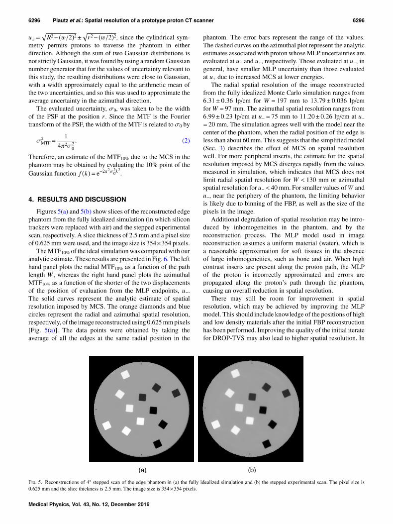
Figures 5(a) and 5(b) show slices of the reconstructed edgephantom from the fully idealized simulation (in which silicontrackers were replaced with air) and the stepped experimentalscan, respectively. A slice thickness of 2.5 mm and a pixel sizeof 0.625 mm were used, and the image size is 354×354 pixels.

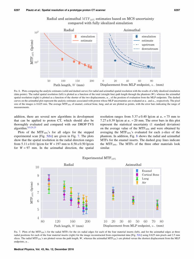
The MTF10% of the ideal simulation was compared with ouranalytic estimate. These results are presented in Fig. 6. The lefthand panel plots the radial MTF10% as a function of the pathlength W , whereas the right hand panel plots the azimuthalMTF10% as a function of the shorter of the two displacementsof the position of evaluation from the MLP endpoints, u−.The solid curves represent the analytic estimate of spatialresolution imposed by MCS. The orange diamonds and bluecircles represent the radial and azimuthal spatial resolution,respectively, of the image reconstructed using 0.625 mm pixels[Fig. 5(a)]. The data points were obtained by taking theaverage of all the edges at the same radial position in the

phantom. The error bars represent the range of the values.The dashed curves on the azimuthal plot represent the analyticestimates associated with proton whose MLP uncertainties areevaluated at u− and u+, respectively. Those evaluated at u−, ingeneral, have smaller MLP uncertainty than those evaluatedat u+ due to increased MCS at lower energies.

The radial spatial resolution of the image reconstructedfrom the fully idealized Monte Carlo simulation ranges from6.31± 0.36 lp/cm for W = 197 mm to 13.79± 0.036 lp/cmfor W = 97 mm. The azimuthal spatial resolution ranges from6.99±0.23 lp/cm at u−= 75 mm to 11.20±0.26 lp/cm at u−= 20 mm. The simulation agrees well with the model near thecenter of the phantom, when the radial position of the edge isless than about 60 mm. This suggests that the simplified model(Sec. 3) describes the effect of MCS on spatial resolutionwell. For more peripheral inserts, the estimate for the spatialresolution imposed by MCS diverges rapidly from the valuesmeasured in simulation, which indicates that MCS does notlimit radial spatial resolution for W < 130 mm or azimuthalspatial resolution for u−< 40 mm. For smaller values of W andu−, near the periphery of the phantom, the limiting behavioris likely due to binning of the FBP, as well as the size of thepixels in the image.

Additional degradation of spatial resolution may be intro-duced by inhomogeneities in the phantom, and by thereconstruction process. The MLP model used in imagereconstruction assumes a uniform material (water), which isa reasonable approximation for soft tissues in the absenceof large inhomogeneities, such as bone and air. When highcontrast inserts are present along the proton path, the MLPof the proton is incorrectly approximated and errors arepropagated along the proton’s path through the phantom,causing an overall reduction in spatial resolution.

There may still be room for improvement in spatialresolution, which may be achieved by improving the MLPmodel. This should include knowledge of the positions of highand low density materials after the initial FBP reconstructionhas been performed. Improving the quality of the initial iteratefor DROP-TVS may also lead to higher spatial resolution. In

F. 5. Reconstructions of 4◦ stepped scan of the edge phantom in (a) the fully idealized simulation and (b) the stepped experimental scan. The pixel size is0.625 mm and the slice thickness is 2.5 mm. The image size is 354×354 pixels.

Medical Physics, Vol. 43, No. 12, December 2016

6297 Plautz et al.: Spatial resolution of a prototype proton CT scanner 6297

F. 6. Plots comparing the analytic estimates (solid and dashed curves) for radial and azimuthal spatial resolution with the results of a fully idealized simulation(data points). The radial spatial resolution (left) is plotted as a function of the total (straight line) path length through the phantom (W ), whereas the azimuthalspatial resolution (right) is plotted as a function of the shorter of the two displacements, u−, of the position of evaluation from the MLP endpoints. The dashedcurves on the azimuthal plot represent the analytic estimates associated with proton whose MLP uncertainties are evaluated at u− and u+, respectively. The pixelsize of the images is 0.625 mm. The average MTF10% of enamel, cortical bone, lung, and air are plotted as points, with the error bars indicating the range ofmeasurements.

addition, there are several new algorithms in developmentthat can be applied to proton CT, which should also bethoroughly evaluated and compared with our DROP-TVSalgorithm.8,9,24,25

Plots of the MTF10%’s for all edges for the steppedexperimental scan [Fig. 5(b)] are given in Fig. 7. The plotsshow that the spatial resolution in the radial direction rangesfrom 5.11±0.61 lp/cm for W = 197 mm to 8.58±0.50 lp/cmfor W = 97 mm. In the azimuthal direction, the spatial

resolution ranges from 5.37±0.40 lp/cm at u− = 75 mm to7.27±0.39 lp/cm at u−= 20 mm. The error bars in this plotrepresent the statistical uncertainty (1 standard deviation)on the average value of the MTF10% and were obtained byaveraging the MTF10%’s evaluated for each z-slice of thephantom. In addition, Fig. 8 shows the radial and azimuthalMTFs for the enamel inserts. The dashed gray lines indicatethe MTF10%. The MTFs of the three other materials looksimilar.

F. 7. Plots of the MTF10%’s for the radial MTFs for the six radial edges for each of the four material inserts (left), and for the azimuthal edges at threeradial positions for each of the four material inserts (right) for the image reconstructed from experimental data [Fig. 5(b)] using 0.625 mm pixels and 2.5 mmslices. The radial MTF10%’s are plotted versus the path length, W , whereas the azimuthal MTF10%’s are plotted versus the shortest displacement from the MLPendpoints, u−.

Medical Physics, Vol. 43, No. 12, December 2016

6298 Plautz et al.: Spatial resolution of a prototype proton CT scanner 6298

F. 8. (a) The radial MTFs for the six radial enamel edges. (b) The azimuthal MTFs for three azimuthal enamel edges. The horizontal dashed lines in eachfigure indicate the MTF10%.

As expected MTF10%’s show strong dependence on pathlength and position of evaluation, for radial and azimuthaledges, respectively, and little material dependence. Althoughthe effect is not large, in the radial plot, it appears that thehigh density inserts, enamel and cortical bone, tend to haveconsistently lower spatial resolution than the low densityinserts, air and lung. This may be understood in terms ofthe amount of scattering the different density materials cause,which affects the MLPs in different ways. Scattering will belargest for the high-density materials (bone and enamel), andfor lower proton energies at smaller radial displacements. Thematerial dependence of the azimuthal edge resolution is evenless pronounced than that of the radial edge distributions. Thismay be because the geometry of the phantom is such that highand low density inserts are always opposite to one another,

and so reduced scattering in the low density inserts maybe counteracted by increased scattering in the high densityinserts.

Figure 9 shows a comparison between the MTF10% valuesof the most ideal simulation, the simulation with the realisticsilicon tracker, the stepped experimental scan and the contin-uous experimental scan. The plot shows strong agreementbetween the idealized simulation with the silicon tracker andthe two experimental scans. Evidently, replacing the idealtracking detectors with silicon detectors significantly reducedthe spatial resolution overall, ranging from a reduction of20% for W = 197 mm to 37% for W = 97 mm. This is becausethe MLP model assumes exact knowledge of the entry andexit points from the phantom, whereas due to MCS andpoint resolution uncertainty in the silicon trackers, the MLP

F. 9. A comparison between the fully idealized simulation, the simulation with the realistic silicon tracker, the stepped experimental scan and the continuousexperimental scan. The average MTF10% of enamel, cortical bone, lung, and air are plotted, with the error bars indicating the range of measurements. The pixelsize in the images is 0.625 mm.

Medical Physics, Vol. 43, No. 12, December 2016

6299 Plautz et al.: Spatial resolution of a prototype proton CT scanner 6299

endpoints are fairly uncertain. This increases the uncertaintyat every point along the MLP curve, with the most significantincrease occurring near the endpoints, where the uncertaintyis zero in the ideal case. This results in the largest reduction inspatial resolution occurring near the periphery of the phantom,(small W and u−) as is indicated by the plots.

In addition, the azimuthal resolution is reduced by about5% more than the radial resolution near the periphery of thephantom. This is expected because the protons that contributethe largest uncertainty at these points have much larger W thantheir radial counterparts, resulting in the azimuthal protonshaving less residual energy when they enter the rear tracker.Because of this, they are subject to a greater amount of MCSin the rear tracker than protons with higher residual energy.

As indicated by Fig. 9, the range of MTF values fromcontinuous experimental scan, and simulated and experi-mental stepped scans overlapped for both radial and azimuthalresolutions. This means that a stepped scan with 4◦ stepsgives equivalent results in terms of spatial resolution, whichis important when the proton beam is pulsed (as is the casefor synchrotrons) and thus continuous scans are not optimal.

5. CONCLUSIONS

We have characterized the spatial resolution of a prototypeproton CT system by comparing an analytic estimate withtwo simulated systems at various levels of idealization,and with two experimental scans. We have demonstratedan understanding of how each component of the prototypesystem affects the spatial resolution of a proton CT image.Comparison of the fully idealized simulation with the analyticestimate suggests that near the center of the phantom, thespatial resolution is limited by MCS; however, for path lengthsof less than approximately 130 mm, other factors are morelimiting than MCS. It may still be possible to further improvespatial resolution by using an improved MLP estimate and/oran improved initial iterate from DROP-TVS. Comparing themore realistic simulation and the experimental results withthe fully idealized simulation reveals that MCS in the silicondetectors is the largest contributor to the degradation ofspatial resolution, which poses a convincing case for a moretransparent proton tracking system. Since the silicon waferswere left over from a previous and unrelated project,26 theirdesign was not optimized for application in proton CT. Apreferable design may use 200 µm thick double sided silicondetectors, which would reduce the amount of material bya factor of 4. The strip pitch of the SSDs also results ina small reduction in spatial resolution due to uncertaintyin the coordinate measurement. This could be reduced byusing SSDs with a finer pitch, but it is a fairly insignificanteffect compared with the thickness of the detectors and wouldincrease the complexity of the detector readout.

In order to further improve spatial resolution of proton CT,we suggest to develop more transparent tracking detectors,and to implement improved path estimation algorithms. Thesemay include starting from a more advanced FBP algorithm,and the incorporation of information about heterogeneities in

the MLP formalism of the subsequent iterative reconstruction.Finally, the development and availability of higher-energymedical accelerators for protons as well as for heavier ionswill lead to images with improved spatial resolution.

ACKNOWLEDGMENTS

The authors acknowledge Caesar Ordoñez (NorthernIllinois University) for assisting with preprocessing of contin-uously scanned data, and with image reconstruction. They alsoacknowledge the contributions of Yair Censor (The Universityof Haifa, Israel) and Scott Penfold (University of Wollongong,Australia). They acknowledge the crucial support from MarkPankuch and the accelerator operating staff at NorthwesternMedicine Chicago Proton Center. Finally, they acknowledgeJosé Ramos Mendez (U.C. San Francisco) for implementingthe proton CT scanner geometry in and TheodoreGeoghegan (U.C. San Francisco) for running the simulationsthat were used in this study. The research in proton CThas been supported by the National Institute of BiomedicalImaging and Bioengineering (NIBIB), and the NationalScience Foundation (NSF), Award No. R01EB013118. Thecontent of this paper is solely the responsibility of the authorsand does not necessarily represent the official views of NIBIB,NIH, and NSF.

CONFLICT OF INTEREST DISCLOSURE

The authors have no COI to report.

a)Author to whom correspondence should be addressed. Electronic mail:tiaplautz@gmail.com

1G. Poludniowski, N. M. Allinson, and P. M. Evans, “Proton radiography andtomography with application to proton therapy,” Br. J. Radiol. 88, 20150134(2015).

2U. Schneider and E. Pedroni, “Proton radiography as a tool for qualitycontrol in proton therapy,” Med. Phys. 22, 353–363 (1995).

3J. L. Romero et al., “Patient positioning for proton therapy using a protonrange telescope,” Nucl. Instrum. Methods Phys. Res., Sect. A 356, 558–565(1995).

4R. P. Johnson, J. DeWitt, C. Holcomb, S. Macafee, H. F.-W. Sadrozin-ski, and D. Steinberg, “Tracker readout ASIC for proton computedtomography data acquisition,” IEEE Trans. Nucl. Sci. 60, 3262–3269(2013).

5R. P. Johnson, V. Bashkirov, L. DeWitt, V. Giacometti, R. F. Hurley, P.Piersimoni, T. E. Plautz, H. F.-W. Sadrozinski, K. Schubert, R. W. Schulte,B. Schultze, and A. Zatserklyaniy, “A fast experimental scanner for protonCT: Technical performance and first experience with phantom scans,” IEEETrans. Nucl. Sci. 63, 52–60 (2015).

6V. A. Bashkirov, R. W. Schulte, R. F. Hurley, R. P. Johnson, H. F.-W. Sadrozinski, A. Zatserklyaniy, T. Plautz, and V. Giacometti, “Novelscintillation detector design and performance for proton radiography andcomputed tomography,” Med. Phys. 43, 664–674 (2016).

7S. N. Penfold, R. W. Schulte, Y. Censor, V. Bashkirov, S. McAllister, K.Schubert, and A. B. Rosenfeld, “Block-iterative and string-averaging projec-tion algorithms in proton computed tomography image reconstruction,”http://ro.uow.edu.au/engpapers/1856/, 2010.

8S. Rit, G. Dedes, N. Freud, D. Sarrut, and J. M. Létang, “Filtered backpro-jection proton CT reconstruction along most likely paths,” Med. Phys. 40,031103 (9pp.) (2013).

9D. C. Hansen, N. Bassler, T. S. Sørensen, and J. Seco, “The image qualityof ion computed tomography at clinical imaging dose levels,” Med. Phys.41, 111908 (10pp.) (2014).

Medical Physics, Vol. 43, No. 12, December 2016

6300 Plautz et al.: Spatial resolution of a prototype proton CT scanner 6300

10R. W. Schulte, S. N. Penfold, J. T. Tafas, and K. E. Schubert, “A maximumlikelihood proton path formalism for application in proton computed tomog-raphy,” Med. Phys. 35, 4849–4856 (2008).

11D. C. Williams, “The most likely path of an energetic charged par-ticle through a uniform medium,” Phys. Med. Biol. 49, 2899–2911(2004).

12B. Schaffner, E. Pedroni, and A. Lomax, “Dose calculation models for pro-ton treatment planning using a dynamic beam delivery system: An attemptto include density heterogeneity effects in the analytical dose calculation,”Phys. Med. Biol. 44, 27–41 (1999).

13I. Mori and Y. Machida, “Deriving the modulation transfer function of CTfrom extremely noisy edge profiles,” Radiol. Phys. Tech. 2, 22–32 (2009).

14J. Seco, M. Oumano, N. Depauw, M. F. Dias, R. P. Teixeira, and M. F.Spadea, “Characterizing the modulation transfer function (MTF) of pro-ton/carbon radiography using Monte Carlo simulations,” Med. Phys. 40,091717 (8pp.) (2013).

15U. Schneider, E. Pedroni, M. Hartmann, J. Besserer, and T. Lomax, “Spatialresolution of proton tomography: Methods, initial phase space and objectthickness,” Z. Med. Phys. 22, 100–108 (2012).

16S. Agostinelli et al., “4: A Simulation toolkit,” Nucl. Instrum. MethodsPhys. Res., Sect. A 506, 250–303 (2003).

17“User guide for version 2.0,” http://www.topasmc.org/user-guide,2015.

18J. Perl, J. Shin, J. Schümann, B. Faddegon, and H. Paganetti, “: Aninnovative proton Monte Carlo platform for research and clinical applica-tions,” Med. Phys. 39, 6818–6837 (2012).

19L. A. Feldkamp, L. C. Davis, and J. W. Kress, “Practical cone-beam algo-rithm,” J. Opt. Soc. Am. A 1, 612–619 (1984).

20S. N. Penfold, R. W. Schulte, Y. Censor, and A. B. Rosenfeld, “Totalvariation superiorization schemes in proton computed tomography imagereconstruction,” Med. Phys. 37, 5887–5895 (2010).

21P. F. Judy, “The line spread function and modulation transfer function of acomputed tomographic scanner,” Med. Phys. 3, 233–236 (1976).

22H. Fujita et al., “A simple method for determining the modulation transferfunction in digital radiography,” IEEE Trans. Med. Imaging 11, 34–39(1992).

23“ language reference, version 2.7,” http://www.python.org, 2016.24D. Kim, S. Ramani, and J. A. Fessler, “Combining ordered subsets and

momentum for accelerated X-ray CT image reconstruction,” IEEE Trans.Med. Imaging 34, 167–178 (2015).

25N. T. Karonis, K. L. Duffin, C. E. Ordoñez, B. Erdelyi, T. D. Uram, E. C. Ol-son, G. Coutrakon, and M. E. Papka, “Distributed and hardware acceleratedcomputing for clinical medical imaging using proton computed tomography(pCT),” J. Parallel Distrib. Comput. 73, 1605–1612 (2013).

26W. B. Atwood et al., “The large area telescope on the Fermi gamma-rayspace telescope mission,” Astrophys. J. 697, 1071–1102 (2009).

Medical Physics, Vol. 43, No. 12, December 2016