an examination of alternative compensation …
TRANSCRIPT

AN EXAMINATION OF ALTERNATIVE
COMPENSATION METHODS FOR THE REMOVAL OF THE
RIDGING EFFECT FROM DIGITAL TERRAIN MODEL
DATA FILES
KEVIN HUNTLY PEGLER
October 2001
TECHNICAL REPORT NO. 217
TECHNICAL REPORT NO. 209

AN EXAMINATION OF ALTERNATIVE COMPENSATION METHODS FOR THE
REMOVAL OF THE RIDGING EFFECT FROM DIGITAL TERRAIN MODEL DATA FILES
Kevin Huntly Pegler
Department of Geodesy and Geomatics Engineering University of New Brunswick
P.O. Box 4400 Fredericton, N.B.
Canada E3B 5A3
October 2001
© Kevin H. Pegler, 1999

PREFACE
In order to make our extensive series of technical reports more readily available, we have scanned the old master copies and produced electronic versions in Portable Document Format. The quality of the images varies depending on the quality of the originals. The images have not been converted to searchable text.

PREFACE
This technical report is a reproduction of a report submitted in partial fulfillment of the
requirements for the degree of Master of Engineering in the Department of Geodesy and
Geomatics Engineering, September 1999. This work was supported by Service New
Brunswick. The research was supervised by Dr. David Coleman.
As with any copyrighted material, permission to reprint or quote extensively from this
report must be received from the author. The citation to this work should appear as follows:
Pegler, K. H. (200 1 ). An Examination of Alternative Compensation Methods for the Removal of the Ridging Effect from Digital Terrain Model Data Files. M.Eng. report, Department of Geodesy and Geomatics Engineering Technical Report No. 209, University ofNew Brunswick, Fredericton, New Brunswick, Canada, 173 pp.

ABS1RACT
The province ofNew Brunswick began a systematic program of province-wide Digital
Terrain Model (DTM) coverage in the late-1980's. Using 1:35,000-scale aerial
photography, the DTMs were collected photogrammetrically as a series of profiles spaced
70 metres apart. No regard was given to brealdines along roads or water bodies.
The DTMs have gone through a series of stringent quality control checks to eliminate
blunders and ensure the elevations of data points are blunder-free and all fiill within
specified accuracy tolerances. However, users of these DTM's have continued to express
concern over perceived data quality based on the evidence of a regular "ridging" effect
within many of the DTM files when viewed under certain conditions. Aware of similar
phenomena found in DTMs produced by other organizations, Service New Brunswick
(SNB) commissioned researchers in the Department of Geodesy and Geomatics
Engineering at the University ofNew Brunswick to investigate the respective
requirements and ahernatives for batch processing of the DTMs to remove this ridging
effect.
This report presents research examining specific technical issues and compensation
approaches associated with the quantification and removal of the ridging phenomena
found in SNB's Enhanced Topographic Database digital terrain data. Further, the issue of
ridging will be investigated from poihts of view ranging from a data limitation issue to a
visualization issue. Firlally, up to five specific solhtions will be examined and compared.
11

ACKNOWLEDGEMENTS
As in any similar undertaking, there are many people to thank. First of all, I would like
to thank my supervisor, Dr. David J. Coleman. His guidance and support have been
crucial to the development and completion of this report. As a mentor, I can say of Dave
that ''they just do not get any better than that!" All his efforts are greatly appreciated.
This work would not have been possible without the financial assistance of the
Province ofNew Brunswick, through Service New Brunswick. In particular, I would to
thank Mr. Rejean Castonguay who sat patiently through what seemed like an endless
stream of''progress meetings." He always showed a great interest in all our successes and
equally in all our :fiillures. Moreover, Rejean's advice, based on his many years of
experience, was very helpful and very much appreciated.
I have always said that I am doing this degree for my children. Although, they are too
young to realize it now, in the years to come I want them to know that all the sacrifice is
intended to open future doors for them. I want them to reach for the stars.
Finally, I would like to acknowledge the sacrifice and efforts of my wife Shirley. Since
her arrival in my life, she has provided the catalyst that allows me to achieve ever higher
goals. I love her very much and look forward to our "continuing adventure!"
lll

TABLE OF CONTENTS
PAGE
Abstract . . . . . . . . . . . . . . . . . . . . . . . . . . . . . . . . . . . . . . . . . . . . . . . . . . . . . . . . . . . . . ii Acknowledgements . . . . . . . . . . . . . . . . . . . . . . . . . . . . . . . . . . . . . . . . . . . . . . . . . . . iii Table of Contents . . . . . . . . . . . . . . . . . . . . . . . . . . . . . . . . . . . . . . . . . . . . . . . . . . . . iv List of Tables . . . . . . . . . . . . . . . . . . . . . . . . . . . . . . . . . . . . . . . . . . . . . . . . . . . . . . . . vii L. fF" ... tSt o 1gures . . . . . . . . . . . . . . . . . . . . . . . . . . . . . . . . . . . . . . . . . . . . . . . . . . . . . . V111
1.0 INTRODUCTION .............................................. 1
1.1 Project Objectives . . . . . . . . . . . . . . . . . . . . . . . . . . . . . . . . . . . . . . . . . . 5 1.2 Proposed Approach ........................................ 6
1.2.1 Background Research . . . . . . . . . . . . . . . . . . . . . . . . . . . . . . . . . 6 1.2.2 Test Procedures to Identify the Existence of"Ridging" within a
Dataset ............................................ 7 1.2.3 Development of a ''Testing Criteria ....................... 7 1.2.4 Test and Develop Alternative Solutions for the Compensation of
Ridging Within a Dataset . . . . . . . . . . . . . . . . . . . . . . . . . . . . . . 7 1.3 Project Constraints . . . . . . . . . . . . . . . . . . . . . . . . . . . . . . . . . . . . . . . . . 8 1.4 Organization of the Report ................................... 9 1.5 Chapter Summary . . . . . . . . . . . . . . . . . . . . . . . . . . . . . . . . . . . . . . . . . 10
2.0 BACKGROUND RESEARCH ................................... 11
2.1 Manual Profiling - a DTM Data Collection Technique . . . . . . . . . . . . . 11 2.2 Causes of the Ridging Effect- The data limitations Perspective ....... 13 2.3 Causes of the Ridging Effect - The Visualization Limitations Perspective 16 2.4 Spatial Filtering . . . . . . . . . . . . . . . . . . . . . . . . . . . . . . . . . . . . . . . . . . 17 2.5 Fourier Transforms ........................................ 23 2.6 TIN Random Densification .................................. 27 2. 7 Trend Surface . . . . . . . . . . . . . . . . . . . . . . . . . . . . . . . . . . . . . . . . . . . . 28 2.8 Chapter Summary ......................................... 29
lV

3.0 ANALYSIS: DESIGN AND APPROACH .......................... 30
3.0 Analysis: Phase I ......................................... 30 3.1 Approach ............................................... 30
3.1.1 Study Site Selection ................................. 30 3.1.2 Software Selection .................................. 32 3.1.3 Test Patch Creation .................................. 32 3.1.4 Development of the Testing Criteria ..................... 33 3.1.5 Investigation into the Automatic Detection ofRidging ....... 38
3.2 Development of Solutions for the Ridging Phenomena ............. 41 3.2.1 Spatial Filtering ..................................... 41 3.2.2 TIN Random Densification ............................ 43 3.2.3 Fourier Transformation ............................... 49 3.2.4 Trend Surface ...................................... 52
3.3 Analysis: Phase II ......................................... 52 3.4 Approach Phase II ........................................ 53 3.5 Chapter SllJlllllalY ......................................... 53
4.0 ANALYSIS AND DISCUSSION OF RESULTS ..................... 55
4.1 Subjective and Analytical Analysis ............................ 55 4.2 Phase I Resuhs . . . . . . . . . . . . . . . . . . . . . . . . . . . . . . . . . . . . . . . . . . . 56
4.2.1 Investigation into Histogram of Aspect Values . . . . . . . . . . . . . 56 4.2.2 3D Visualization Analysis . . . . . . . . . . . . . . . . . . . . . . . . . . . . . 60
4.2.2.1 LPF Spatial Filtering ........................... 61 4.2.2.2 Fourier Filtering . . . . . . . . . . . . . . . . . . . . . . . . . . . . . . 62 4.2.2.3 TIN Random Densification ...................... 62 4.2.2.4 Trend Surface . . . . . . . . . . . . . . . . . . . . . . . . . . . . . . . . 63
4.2.3 Profile Analysis . . . . . . . . . . . . . . . . . . . . . . . . . . . . . . . . . . . . . 64 4.2.3 .1 LPF Spatial Filtering . . . . . . . . . . . . . . . . . . . . . . . . . . . 64 4.2.3.2 Fourier Filtering .............................. 64 4.2.3.3 TIN Random Densification ...................... 65 4.2.3.4 Trend Surface ................................ 66
4.2.4 100 Random Point Comparison ......................... 66 4.2.4.1 LPF Spatial Filtering ........................... 68 4.2.4.2 Fourier Transformations ........................ 69 4.2.4.3 TIN Random Densification . . . . . . . . . . . . . . . . . . . . . . 71 4.2.4.4 Trend Surface ................................ 72
4.2.5 Implications of the Resuhs ............................ 73 4.2.6 Phase I Analysis Decisions and Discussion ................ 75
4.3 Phase II Results . . . . . . . . . . . . . . . . . . . . . . . . . . . . . . . . . . . . . . . . . . 76
v

4.3.1 Contouring ........................................ 77 4.3.2 100 Random Point Comparison ......................... 80 4.3.3 Hydrological Analysis ................................ 83 4.3.4 Phase II Analysis Decisions and Discussion ................ 84
4.4 Implementation Considerations . . . . . . . . . . . . . . . . . . . . . . . . . . . . . . . 85 4.5 Chapter Summary . . . . . . . . . . . . . . . . . . . . . . . . . . . . . . . . . . . . . . . . . 86
5.0 CONCLUSIONS .............................................. 87
5.1 Review ofProject Objectives ................................ 87 5.2 Summary ofTesting Results ................................. 89
5.2.1 Phase I Testing Results .............................. 90 5.2.2 Phase II Testing Results .............................. 91
5.3 Future Research .......................................... 92 5.2 Concluding Remarks ...................................... 93
REFERENCES ..................................................... 94
BffiLIOGRAPHY ................................................... 97
APPENDICES
A. Avenue Script: Ridge_Detector.ave ................................. 98 B. Avenue Script: TIN_RD.ave ..................................... 105 C. Avenue Script: TREND.ave ...................................... 114 D. Analysis: Phase I - DTM Plots . . . . . . . . . . . . . . . . . . . . . . . . . . . . . . . . . . . . 117 E. Analysis: Phase II - DTM Plots . . . . . . . . . . . . . . . . . . . . . . . . . . . . . . . . . . . 140 F. Histograms . . . . . . . . . . . . . . . . . . . . . . . . . . . . . . . . . . . . . . . . . . . . . . . . . . 144 G. Scatter Plots ................................................. 149 H. Analysis: Phase II - Contour Plots . . . . . . . . . . . . . . . . . . . . . . . . . . . . . . . . . 159 I. Analysis: Phase II - Hydrological . . . . . . . . . . . . . . . . . . . . . . . . . . . . . . . . . . 163
vi

LIST OF TABLES
MAIN BODY PAGE
4-1 Summary of Phase I Objective Analysis .............................. 60 4-2 Phase I, 100 Random Point Comparison .............................. 66 4-3 Summary of Contouring Analysis ................................... 79 4-4 Phase II, 100 Random Point Comparison . . . . . . . . . . . . . . . . . . . . . . . . . . . . . 80 4-5 Phase II, Slope based 100 Random Point Comparison ................... 82
vii

LIST OF FIGURES
MAIN BODY PAGE
1-1 Example of ridging in SNB DTM dataset. Caraquet, New Brunswick. ........ 3 1-2 Ridging in a USGS dataset. Mount St. Helens, Washington State.. . ......... 3 1-3 Competing philosophies in the cause of the riding phenomena. .............. 5 2-1 Manual Profiling. . . . . . . . . . . . . . . . . . . . . . . . . . . . . . . . . . . . . . . . . . . . . . . . 12 2-2 Example of ridging over a peat bog. Caraquet, N.B ...................... 15 2-3 Presence of ridging in areas of high relief. Hayesville, N.B ................. 15 2-4 Horizontal linear array of TIN fucets representing ridging . . . . . . . . . . . . . . . . . 17 2-5 An example of ridging as a high frequency phenomenon. ................. 18 2-6 Operation of a low pass filter. . . . . . . . . . . . . . . . . . . . . . . . . . . . . . . . . . . . . . 19 2-7 Ridging removal process using FFT' s. . . . . . . . . . . . . . . . . . . . . . . . . . . . . . . . 26 3-1 Study site locations. . . . . . . . . . . . . . . . . . . . . . . . . . . . . . . . . . . . . . . . . . . . . . 31 3-2 Contours generated from DTM containing ridging ...................... 38 3-3 Contours generated from filtered DTM .............................. 38 3-4 TIN fucet alignment in the vicinity of riding, Aroostook, N.B .............. 39 3-5 Histogram of aspect values ..................................... 39 3-6 Ridging Detection- User Interfuce .................................. 40 3-7 The process of TIN random densification. ............................ 44 3-8 Unfiltered TIN. Peat Bog, Caraquet, N.B ............................. 47 3-9 Randomly Densified TIN with the original mass point data included . . . . . . . . . 4 7 3-10 Randomly Densified TIN with the original mass point data removed . . . . . . . . . 48 3-11 Magnitude image, DTM transformed to the frequency domain. ............ 51 3-12 Bit map editing in the frequency domain. ............................. 51 4-1 Histogram - aspect of unfiltered DTM, Caraquet, N .B. . . . . . . . . . . . . . . . . . . . 57 4-2 Histogram- aspect of TIN Random Densification, Caraquet, N.B. . ........ 57 4-3 Histogram- aspect of unfiltered DTM, Aroostook, N.B. . ................ 59 4-4 Histogram- aspect of TIN Random Densification, Caraquet, N.B ........... 59 4-5 Scatter Plot ofLPF v. Unfiltered Elevations, Aroostook, N.B .............. 68 4-6 Scatter Plot ofFourier v. Unfiltered Elevations, Aroostook, N.B ............ 70 4-7 Scatter Plot of TIN Random Densification v. Unfiltered Elevations, Caraquet,
N.B .......................................................... 72 4-8 Scatter Plot of Trend Surfuce v. Unfiltered Elevations, Caraquet, N.B ........ 73 4-9 Relative file sizes for phase I. ...................................... 75 4-10 Caraquet, 0.5m contours from unfiltered TIN .......................... 77 4-11 Caraquet, 0.5m contours from TIN processed with TIN random densification . 78 4-12 Caraquet, 0.5m contours from CTM Fourier Filtering ................... 78 4-13 Slope base 100 random point Comparison, Aroostook, N.B. .............. 81
viii

1
JNTRODUCTION
The terms digital elevation model (DEM) and digital terrain model (DTM) are often
used interchangeably. In the late 1950's Miller and LaFJamme of MIT defined DTMs as:
" simply a statistical representation of the continuous surfuce of the ground by a large number of selected points with known xyz coordinates in an arbitrary coordinate :field"[1958].
The term DEM is defined by Bonham-Carter as a " digital computer file containing a
grid or MATRIX of elevation models"[1994]. Ahhough these terms are often confused in
industry, these definitions will be used for this report. The term DTM is the more general
term that can be used to describe any digital representation of terrain. The term DEM, as
defined here, can only be used to define those digital representations of terrain that are
collected as regularly spaced lattice of points or cells of elevation values. A DEM is a
DTM but, a DTM is not necessarily aDEM. Except for specific instances, the term DTM
will be used.
Digital Terrain Models (DTM) have proven useful to applications in hydrological
modelling, geophysical data manipulation, spatial analysis within a Geographic
Information System (GIS), viewshed analysis for forestry management systems, and GIS
for transportation systems (GIS-T). Digital Elevation Models can be thought of as a
fundamental set within the geomatics community - much like the topographic mapping
produced by the large base mapping programs of the 1970's. DTMs are utilized by most of
1

the communities associated with geomatics including: civil engineering, forestry,
surveying, planning, geology, geography and corporate strategic decision makers,
although for very different purposes.
In order to promote development activities, governments across North America collect
and sell DTM datasets. It is important that the quality of the DTM product is good in
order that user groups develop a high regard for the data. A product perceived to have
high quality will develop a good market for itself and this speeds recovery of the
production costs.
Concern arises in government agencies when users perceive that the data sets being
purchased are flawed. Such is the case with Service New Brunswick's (SNB) Digital
Terrain Model Database. While the data was collected to a high accuracy ( DTM points
are within 2.5 metres of their true elevation) and have undergone rigorous quality control
processes [NBGIC, 1995] , users have reported in certain 3-Dimensional perspective
views a geometric effect in the DTM data which manifests itself as a series of ridges. The
''ridging" runs in generally a north/south direction and is most prevalent in regions having
little topographic relief. The magnitude of the ridges is less than 10 metres. Figure 1-1
illustrates the ridging within a SNB DTM dataset.
2

Figure 1-1: Example of ridging in SNB DTM dataset. Caraquet, New Brunswick.
The SNB DTM datasets are not the only DTM datasets contaminated by the
ridging effect. Researcher has indicated that "banding" or, "striping" also exists in USGS
7112-Minute DEM datasets- as shown in Figure 2-2 [Isaacson and Ripple, 1990].
Figure 1-2: Example ofRidging in USGS datasets. Mount St. Helens, Washington State. 3

USGS and SNB DTM data were collected having the mass points sampled along regu]arly
spaced profile lines. Moreover, the stereoplotter operator collected the lines in a
"shuttlecock" manner. That is to say, the data was collected up they-axis on one line and
then downy-axis of the next- just as a field is plowed. The result is a DTM data set
comprising row upon row of points of elevation values. The USGS believes that their
"striping" or as it is called here, ''ridging" is a ''form of systematic error process which
commonly affects photogrammetric digital elevation data"[Brown and Bara, 1994].
In order to find the solution to an effect such as ridging in DTMs, first the cause must
be determined. At the earliest stages of research, it was postulated that ridging was an
artifuct of: ( 1) some combination of systematic errors incurred during the data collection
process; (2) the pattern and/or distnoution ofDTM points along regularly-spaced profile
lines; or (3) some combination of(1) and (2)[Coleman, 1998].
Moreover, there are those who subscribe to the philosophy that ridging is a data
limitation problem. They believe that ridging is caused by systematic errors introduced by
the operator when collecting the data along profile lines. At the other end of the spectrum,
it has been proposed that the ridging is due solely to the linear arrangement of the point
data. Proponents believe it is the linear aligmnent of the mass points which causes the
visualization of the ridges and not some systematic error introduced at the time of data
collection. Figure 1-3 graphically illustrates the range of philosophies.
4

Data Limitations -poor quality or, containing errocs.
Ridging Effect
Visualization Limitations -illogical modelling of terrain or, unnatural visualization techniques.
Figure 1-3: Competing philosophies in the cause of the ridging phenomena.
There was sufficient concern on the part of SNB that researchers at the Department of
Geodesy and Geomatics Engineering at the University ofNew Brunswick were contracted
to investigate the causes and removal methods of the ridging phenomena in SNB DTM
datasets.
1.1 Project Objectives
The principal goal of this research is to find the cause and a method of removal for the
ridging effect from Service New Brunswick DTM files. The secondary objectives of the
project are:
(1) To establish the magnitude of "ridges" and to identifY a criterion of testing for the
DTMdata;
(2) to test procedures to automatically identifY the existence of the ridging effect
within SNB DTM datasets;
(3) to test several alternative filtering procedures to remove or, diminish the ridging
effect;
5

(4) to recommend on the most appropriate method of removal of the ridging and to
develop a strategy for implementation of the necessary changes to the DTM data
files [Pegler and Coleman, 1998].
The purpose of this research is to :first and foremost provide SNB with a method to
detect and then remove ridging from contaminated DTM files. It is hoped that this will
provide a cost effective alternative to recollecting all the data.
The research may also assist other agencies possessing DTM files with similar
characteristics. Although the specifics of their problems may differ it is hoped that this
research can provide a good starting point in solving their problems.
1.2 Proposed Approach
The proposed approach to this research is considered in four separate stages and
presented below in outline form.
1.2.1 Background Research
The Background Research component of the project will cover five tasks, including:
• Meet with SNB personnel to establish lines of communication and begin the
project;
• Review and summarize literature on the ''ridging" effect in digital terrain models to
identify existing research relevant to the SNB problem;
6

• Contact up to five (5) organizations across North America to obtain and compare,
key lessons learned, specifications, and possible solutions with respect to the
ridging effect found in digital terrain datasets.
1.2.2 Test Procedures to Identify the Existence of "Ridging" Within a Dataset
Prior to investigating alternative solutions to the problem, an automated detection
scheme must be tested to determine if a particular dataset contains the ''ridging"
phenomena. This work involves:
• Data collection/conversion and software installation;
• Develop a model for the ''ridging" effect;
• Investigate procedures for the automatic detection of ridging within a dataset.
1.2.3 Development of a "Testing Criteria"
In order to determine practical solutions to the problems resuhing from ridging, a
criteria must be developed defining the key indicators/tolerances for DTM data that
would indicate practical improvements to the datasets in terms of user satisfilction and
economics.
1.2.4 Test and Develop Alternative Solutions for the Compensation of Ridging
Within a Dataset
The uhimate goal of the proposed research is the evaluation of a number of
alternatives for compensating for ''ridging" within DTM datasets. The uhimate solution
7

must be cost effective and provide a practical means of automating a compensation
algorithm. This will allow SNB to improve the quality of 1894 DTM datasets that cover
the province.
The creation of a report on the findings of this research. A progress presentation at the
end of Stage 2 will address the ability to effectively measure the phenomena. Finally, a
presentation of the resuhs to SNB staff will summarize key findings from all of the stages
of the research.
1.3 Project Constraints
For the sake of simplicity, solutions will be developed using commercially available
geomatics software packages. The majority of the work will be performed on a 200MHz
Pentium personal computer having 128 megabytes of RAM, a 2.5 gigabyte hard drive, and
1 gigabyte JAZ drive. The operating system is Microsoft's Wmdows NT 4.0.
It should be reiterated that the goal of the project find the cause and a method of
removal for the ridging effect from Service New Brunswick DTM files. Any software
developed to help solve this problem will be developed and tested in prototype form only
as a ''proof-of-concept". It is not the intention of the researcher to develop a commercial
software package or even an extension to existing commercial software.
8

1.4 Organization of the Report
The report will be organized in the following manner:
• Chapter 1 will provide the context and summarize the problem of ridging in SNB
DTM datasets. The principal objective of the research is stated and secondary
objectives are also described. In addition, the significance of the research is
described. A summary of the proposed approach is presented along with the
constraints of the project.
• Chapter 2 summarizes the relevant background research including the cause of
ridging. In particular, various filtering methods are explored. These include; simple
low pass filtering techniques, Fourier transform filtering, TIN Random
densification and trend surfuces.
• Chapter 3 contains descriptions of the testing procedures to detect ridging, and the
testing criteria for contaminated SNB DTM data. In particular, attention is paid to
indicating practical improvements to the data sets. Further, based on the
improvement criteria, various approaches to eliminate or, reduce ridging are
discussed.
• Chapter 4 contains the summary of analysis, discussion and results obtained in the
investigation undertaken in the previous chapters. In particular, the implications of
the results, analysis decisions and recommendations are presented for the two
phases of testing. Chapter 4 also describes the inclusion of a small pilot project
9

with Computer Terrain Mapping, Boulder Co., who provide a Fourier technique to
filter out ridging primarily for USGS Level-l DEMS.
• The final chapter will contain the summary of analysis, results, and conclusions
obtained in the investigation undertaken in the previous chapters.
1.5 Chapter Summary
On behalf of the province ofNew Brunswick, SNB maintains a province-wide series of
Digital Terrain Models (DTM).The DTMs were collected photogrammetrically as a series
of profiles spaced 70 metres apart.
Users of these DTM's have continued to express concern over perceived data quality
issues based on the evidence of a regu]ar "ridging" effect within many of the DTM files.
There was sufficient concern on the part ofSNB that researchers the University ofNew
Brunswick were contracted to investigate the causes and removal methods of the ridging
phenomena in SNB DTM datasets.
The principal goal of this research is to find the cause and a method of removal for the
ridging effect from Service New Brunswick DTM files. Further, a testing criteria for DTM
data is to be identified. Based on the above findings, up to five alternative filtering
procedures are to be developed to diminish the ridging phenomena.
The following reflect the outcome of this work including: background research,
analysis - design and approach, swnmary analysis and discussion of results, and
conclusions.
10

2
BACKGROUND RESEARCH
A review of the literature demonstrates that the ridging phenomena can be viewed
from two perspectives: (1) that the ridging is due to some data limitation; or (2) that
ridging is a problem due to data arrangement and visualization techniques. In addition, the
background research on ridging identified that similar phenomena existed in other
jurisdictions. Most notable of these is the ridging or, striping phenomena described in the
literature regarding the USGS 7 .5-Minute and 1-Degree Digital Elevation Models.
2.1 Manual Profiling- a DTM Data CoHeetion Technique
The common thread between the USGS DTM and SNB DTM data sets that exhibit
the ridging phenomena is the method in which the mass point data was gathered. In both
cases, the mass point data was collected using a technique called manual profiling.
Figure 2-1 illustrates the manual profiling technique. In this technique, the
stereoplotter operator, gathers the DTM mass points following along regu]arly spaced
profile lines [NBGIC, 1995).
11

Figure 2-l: Manual·Profilillg (Lillesallcl ancl Kiefer ( 19'791 );
At regular spacings along the profile lint; the floating mark is -plaeed on the what the
operator interprets as the surface of the earth. For SNB da~ the interval between the
profile lines is 70 metres and where possible the points are spaced 70m. apart.[NBGIC,
1995]. USGS Levell, 7.5-minute DEMs have a line spacing of90m.and a point spacing
approximately 30 metres [Russel and Ochis, 1996].
The USGS program ofDTM data collection is much larger than the SNB program.
The "Levell" USGS data set collection began in the 1970s. In order to distinguish these
early data sets from those collected with more modem techniques, they are described as
the "Levell" datasets. The majority ofthese data sets were collected using manual
12

profiling techniques [Garbrecht and Starks, 1995]. It is interesting to note that the data
sets collected with more advanced data structures (described as "Level2" datasets) such
as Digital Line Graphs don't exhibit the ridging phenomena [ Garbrecht and Starks, 1995].
In both the USGS and SNB data collection specifications, the majority of the data was
collected along the profiles lines in alternating directions. For example, if the mass points
are being collected along the current profile line in a northerly direction then, upon
completing the run along that line, the operator would move the required spacing to the
next profile line and then begin sampling in a southerly direction. Of course, the
operator's ability to accurately place the floating mark on the earth's surface may be
inhibited by forest canopy cover, water, relief: or problems with the aerial photography
[NBGIC, 1995].
2.2 Causes of the Ridging Effect - The Data Limitations Perspective
In general. the data limitations perspective believes the ridging effect is caused by
some systematic error that is related to the DTM production methods [NBGIC, 1995]. A
common explanation is that the ridging phenomena is due to errors introduced by the
collection of data in a "shuttlecock" or alternate profiling manner [Garbrecht and Starks
1995], [Russel and Ochis, 1996].
Garbrecht and Starks, upon direct consultation with USGS staff: concluded that
ridging is caused by a combination of "human and algorithmic" errors. The human error
manifests itself as different operator perceptions when the floating mark is "set upon" the
ground from between each alternating profile line. Algorithmic errors are introduced by
13

the interpolation algorithm used to interpolate heights between the two profile lines.
Early research into the development of specifications for the production of DTM's
using manual profiling indicated that excessive scanning speed during the collection of
mass points along a profile caused an alternating datum error [Brunson and Olsen, 1980].
Brunson and Olson descnDed the effect as a''herringbone" pattern in the contours derived
from DTMs whose data was collected using ''filst-velocity'' profiling. It was reported that
the herringbone pattern is more prevalent in areas of steep terrain. This type of error is
often referred to as the "lag effect" [Russell, Kumler and Ocbis, 1995]. The datum error
represents a systematic tendency of the photogrammetric operator to allow the :floating
mark to ''fly oft" a crest of a hill and "dig in'' at the base of a hill. The magnitude of this
type of error increases proportionally with the speed of which the operator collects the
data is areas of high relief
Russell, Kumler and Ocbis [1995] in their research suggest that the "lag effect" is not
the sole cause for the systematic error that is said to be manifested by the ridging. If the
lag effect is the sole cause of error in creating ridging, then no ridges would show up in
flat areas. Clearly, Figure 2-2 dispels this notion.
14

Figure 2-2: Example of ridging over a peat bog. Caraquet, N.B. Canada.
Contradicting the finding of Brunson and Olsen, others have found that ridging is often
most prevalent in flat areas [Garbrecht and Starks, 1995] and [Pearson, 1998]. Further,
Figure 2-2 also demonstrates that some profiles are consistently high or low, even where
there is no significant change in elevation. However, the lag effect may explain why, in
rarer instances, ridging is present in areas of steep terrain, as illustrated in Figure 2-3.
Figure 2-3. Presence of Ridging in Areas of High Relief. Hayesville, N.B., Canada.
15

The most recent research representing the data limitations perspective incorporates all
the suggested causes of ridging as listed above. This current definition of the cause of the
ridging phenomena is a function of several :fuctors: manual profiling, algorithm errors,
terrain, "lag effect", operator errors, and machine miscahbration [Russell and Ochis,
1995].
2.3 Causes of the Ridging Effect - The Visualization Limitations Perspective
Those supporting the belief that the ridging is due to limitations in visualization believe
that, at the heart of the matter, it is the linear arrangement of the elevation data [Lee,
1998]. This raises the question, is it logical to attempt to model the earth's chaotic surfuce
using simple linear arrangements of data? From a production point of view, this may
indeed have merit. However, in terms of accurately representing the relief: it is not likely.
One may think of this as being similar to a pair of corduroy trousers. No matter how
worn or smoothed the corduroy is, the lines of corduroy are still visible. Like the
corduroy pants, the data patterns of the SNB DTMs are linear in nature and as a result
visualization of the data will reveal this pattern [Pearson,1998]. In particular, when a TIN
is used to create a DTM based on this data structure, the systematic creation of evenly
spaced triangles of similar dimensions produces a linear pattern when viewed. Figure 2-4
shows the pattern of linear arrays of TIN triangle :fucets created from mass point data
created in a linear manner. Ahhough using TINs to build sur:fuces from nearly regularly
16

,._. .... _:.. . +
; ...... . .if(· -- • ·- •. . +· ~-- .. __ .... ·-·---~ t.·-- __ ._ ............ -~--· f-« .--.. ...... --*·- -:f.
~: •. ~ -~~-·.~-- ... ~~~ .1( .... --~ _._.
.... _._ .__ -~ +-~-- ..._ • - ·-- ~ .. . .. - ··---- .•· -· _.,. .... ., __ ..................
··- -··-- "-·---··--· ·--.. ·~-- -4-· -· .. ---·.
·--- ~ ___ ... _ •·- •··-, --~f:·.
--· .....__ ,. __ -··-··· ~· .---4- ·--· ...___ ·•- ;:
:. .. ~-~---.- ·-·: i- ~~~ ... ~---·-·~~
Figure 2-4: Horizontal linear array ofTIN fucets representing ridging.
sampled data is connnon, the TIN data model was not intended for this purpose. Rather,
it was intended for use with points that clearly define the surfuce but are irregu]arly placed
[Bonham-Carter, 1994]. In filc4 the use ofTINs for manually profiled data sets can
compound the visualization problems.
There are four areas where research has been undertaken to address the ridging
phenomena: spatial fihering, Fourier transformation, TIN random densification and surfuce
interpolation schemes. The background behind each of these approaches will be discussed
in turn.
2.4 Spatial Filtering
''Spatial frequency'' is defined as the measurement of the spatial variation of a
parameter [Schowengerdt, 1997]. For the purposes ofthis work, the parameter being
measured is elevation within a DTM. Spatial :frequency can be classified as either low or
high. Objects that exhibit low :frequency elevations have a slow change of elevation over a
17

small distance [Leblon, 1997]. An example of an object exhibiting a low frequency are
train tracks which exhtbit only a very small change in elevation over a long distance.
An example of an object that exlnbits a high spatial frequency in elevation would be a
series of dykes. The dykes, when viewed in a cross-section, would have rapid changes in
elevation over a short distance [Leblon, 1997]. Ridging is an example of a high frequency
phenomenon, as illustrated in Figure 2-5. The change in elevation is less than 10 metres
over the distance between adjacent DTM profile lines which is approximately 70 metres
[NBGIC,1995].
PnJiile fi'am CARAQUET o48 m Verllclll-ggeqtlon 200X -------r-··------
!
; ! ' ---t--t-f---~-------~-------+-----~--------
i i i . . 1 !
Figure 2-5: An Example of Ridging as a High Frequency Phenomenon.
18

Low pass filters ( LPF ) or, those filters that allow only the lower :frequency objects
through, are used to de-emphasize high :frequency components ofDTMs. Again, ridging
can be reduced by a LPF because it is essentially a high :frequency component of a DTM.
Figure 2-6 illustrates how simple linear 3x3 LPF is implemented.
1 1 1 X {1ft) , 1 ,
Gt~ ~r:--. I ; ' .
.. 1 .. padtl61'1
Orlgt•t ......
1 , 1
~lltiH ......
Figure 2-6: Operation of a Low Pass Filter (after Leblon, [1997])
19

The operation of3x3 LPF is quite simple. A 3x3 kernel is centred over the pixel being
operated on. The unfihered value of the pixel is replaced by the mean of all nine pixels
falling within the kernel The result is a "smoothing" of the rapid changes in elevations - in
the case of an image representing a DTM.
This technique offihering, while a common approach, is known not to be sufficient to
remove all the systematic errors in the DTMs [Brown and Bara, 1994]. Further, the
smoothing effect of the fiher will somewhat degrade the quality of the data by reducing
the peaks and filling in shallow depressions. Of particular concern to many users is that the
shallow depressions representing wet1ands will be smoothed over. Those concerned with
hydrological applications reject this ridging reduction method because of the reduction in
the definition in the outline of drainage features and the introduction of artificial blockages
to drainage channels [Garbrecht and Starks, 1995] Despite its shortcomings, however,
3x3 LPF spatial fihers are often used due to their ease of implementation and simplicity.
There is an important relationship between cell size, fiher size, and dimension of the
feature to be smoothed. In the case of the ridging phenomena in SNB DTM datasets, the
wavelength of the ridging ( ie. crest-to-crest or trough-to-trough) is 140 metres. That
corresponds to the perpendicular distance between three adjacent profile lines. In order for
the fiher to remove the ridge artifBcts, it must extend over the three lines [Leese, 98]. In
order for a 3x3 LPF fiher to smooth the ridge then, the resolution (cell size) of the image
must be resampled to 45 m. If another cell size is being used, then the dimensions of the
fihering kernel ( sometimes referred to as a "boxcar") must be altered to suit the problem.
Researchers suggest that a more robust technique is the use of ''non-square, low pass"
20

filtering techniques [Brown and Bara, 1994]. The non-square filter is oriented
perpendicular to the direction of the ridging in DTM datasets. The filter works in a similar
manner to the 3x3 LPF described above. However, having the kernelS pixels wide and
perpendicular to the ridging allows the filter to smooth a longer wavelength (I..) of the
ridge. In the case ofSNB DTM data that is resampled to 45m resolution, the 3x5 filter
would operate on approximately 1.51.. of a ridge. Orienting the filter perpendicularly to the
ridge allows for greater smoothing across the ridges and less smoothing along the profile
lines where no ridging exists.
Brown and Bara, in their research into the reduction of systematic errors in USGS
DTMs, suggest the use of semivariograms and fractals in the detection of ridges in a DTM
data set. Semivariance is a geostatistical measure which describes a DTM as " ... the
average squared difference of surface values" [ Brown and Bara, 1994) which are a user
defined distance apart. This separation between the values is known as the "lag distance".
The formula for semivariance is as follows:
N-11
r(h) = 112(N-h)L (z(i)-z(i+h)Y i-1
where N is the number of points on the surface, z(i) is the elevation value of the surface at
point i, and z(i+h) is the value of the surface h distance away from point i.
A semivariogram is a plot of semivariance against lag. In general, the smaller the lag
distance the smaller the semivariance and thus the similarity in elevation values. As
reflected in Berry's application of Tobler's 151 law of geography that "all things are
21

related, but nearby things are more related than distant things"[Berry, 1998].
Related to the slope of a log-log plot its semivariance, the fractal dimension of a
surface is a number that ranges between 2 and 3. The formula for the fractal dimension is
as follows:
D= 3- m/2
where the D is the fractal dimension and m is the slope of the log-log plot of semivariance.
The fractal dimension is measure of the self-affinity of a surface [Polidori et al, 1991].
Perhaps self-affinity is best explained with an example. If a drumlin field is modelled by a
DTM, a particular drumlin would possess self-affinity with the rest of the entire field -
regardless of its dimension, scale, and location. It could be thought of as a single drumlin
element in a set of drumlin elements. The quality of the affinity of the drumlin with the rest
of the drumlin field is characterised by its fractal dimension.
In general, DTMs will exhibit self-similarity over short distances - on the order of
hundreds of metres [Brown and Bara, 1994]. Using this property, systematic errors like
ridging may be detected by calculation of the fractal dimension along specific cardinal
directions ie. east/west and north/south. If the fractal number is higher along a particular
direction than its perpendicular counterpart, then this is good evidence as to the existence
and structure of ridging or other systematic errors [Polidori et al, 1991].
Once detected, low pass fihers were used to reduce the systematic error [Brown and
Bara, 1994]. However, this technique also degrades the quality ofDEM by removing data
values which were actually correct. The researchers state " ... that the changes in elevation
22
values with filtering appear to minor ... "[Brown and Bara, 1994]. An investigation into
the contradiction regarding the amount of degradation ofDEM will be performed.
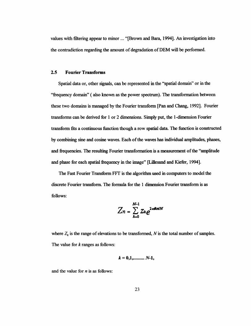
2.5 Fourier Transforms
Spatial data or, other signals, can be represented in the "spatial domain" or in the
''frequency domain" ( also known as the power spectrum). The transformation between
these two domains is managed by the Fourier transform [Pan and Chang, 1992]. Fourier
transforms can be derived for 1 or 2 dimensions. Simply put, the !-dimension Fourier
transform fits a continuous function though a row spatial data. The function is constructed
by combining sine and cosine waves. Each of the waves has individual amplitudes, phases,
and frequencies. The resulting Fourier transformation is a measurement of the "amplitude
and phase for each spatial frequency in the image" [Lillesand and Kiefer, 1994].
The Fast Fourier Transform FFT is the algorithm used in computers to model the
discrete Fourier transform. The formula for the 1 dimension Fourier transform is as
follows:
where Z1 is the range of elevations to be transformed, N is the total number of samples.
The value for kranges as follows:
k = 0,1, ••••••••• N-1,
and the value for n is as follows:
23

n = -N/2, ••••• , N/2
Frederikson [1980] explored the use ofFFfs in the analysis and statistical description
ofDTMs. In his research, particular geological landforms were identified by analysing
DTMs in the frequency domain. Hassan [1998] made use ofFourier transforms for the
identification and filtering of the noise (ridging) within a DTM.
A periodogram is a graph of the power of a signal (or square of the elevation when
transforming a DTM ) versus the frequency. When dea]ing with DTM data, frequency
refers to cycles ( peak-to-peak or, trough-to-trough) per metre rather than cycles per
second [Russell and Ochis, 1996]. The periodogram of a DTM having a smooth surfilce
would exhibit large values at the low frequencies. At the higher frequencies the values
would be extremely small because there would be no rapid change in elevation over a
short distance that is characteristic of high frequency surfilces.
I( however, a sinusoidal wave was introduced to the smooth surfilce of the DTM, an
interesting phenomena occurs. The sinusoidal signal that could represent undulating relief
would produce a spike in the periodogram. This spike would occur at the frequency of the
sine wave introduced to the surfilce.
The Fourier transform bas no way of discriminating signal from noise. The noise in a
DTM will be transferred into the frequency spectrum along with the elevation data. u: however, the noise (or systematic error) bas a particular repeating pattern or wavelength
then, just as with the sinusoidal signal, a spike or spikes will occur at the higher frequency
or frequencies. If these spikes are removed and then the data inversely transformed back
24

to the spatial domain, the systematic error component for the DTM will be removed.
Hassan [1988] is careful to note that not all the random errors or noise will be eliminated
because there may be minor contnbutions to the higher frequency components of the
DTMs that are not eliminated by removing just the major spikes.
Filtering images using Fourier transformations differs from LPF spatial filtering
because it attempts to only remove the systematic error component of an data value and
return only the elevation component. The resulting filtered DTM will be restored with a
minimum of distortions [Hassan, 1988] and will not suffer as great a degradation as occurs
with LPF spatial filtering.
Figure 2-7 illustrates the steps used in the commercial implementation of this process.
The DTM is first separated into individual profile lines that are perpendicular to the
orientation of the ridging. Step 1 in Figure 2-7 illustrates a single profile line. Note the
right hand portion of the profile line is obviously contaminated with ridging. In Step 2, in
the figure, shows the periodogram of the same profile. Notice here that most of the signal
is low-frequency in nature but, that there are two atypical spikes (highlighted by asterisks)
in the higher frequencies. These spikes correspond to the ridging which has a wavelength
of 180 and 90 metres. Note, that this corresponds to the 90 metre distance between DTM
data profiles in USGS 7.5 Minute Levell DTMs.
25

Process
1625
e s I(I(Kl
·"' ~ 1575
1550
.1525+-.......... ~ .................... ---t,__,. 0 2000 4000 1100) ROll)
Di~ance[m)
Unfiltered DEM Power Spectrum Wavelength [ml
10000 100 1000
100
'"i 10 - I l: ~ -1
e:: 10 10~
10 10 I'RqUCncy [ni1 I
Destriped DF..M Power Spectrum
3. \Vavclcngth (m} 4. I (D)() 1000 100 10
1000 16.'i0 Elevation Profile
100 JCil.~
§. 10 e - 1600 !
i ·I 1 1575 e. 10 ··~ ·! 1550 10 .)
10 Ill~ J(J~ 10'1 ur• IS2oli
0 2000 4000 dOOO 8000
Frecp-.eru:y lni1) llimncc[m)
Figure ~7: Ridging Removal Process using FFT's (After Russell et al., [1995]).
The atypical spikes in the high frequencies are then :fihered out. Pan [1989] descnoos
the use of a point filter to remove periodic noise in digital spatial data. The point filter is
multiplied with the frequency domain data and the filtered result is then inversely
transformed back into the spatial domain. The formula for the point filter is as follows:
r'-:::-T
H(u.v) -1.0-e"
26

where (u,v) are the frequency coordinates, a is the standard deviation ofthe Gaussian
distribution and r is as follows:
where (u' ,v') is the frequency of the spike to be removed.
Pan makes the point that, in order not to remove the good data, the user must have
knowledge of the characteristics of the data. For instance, when filtering ridging from
DTMs it is important to understand the wavelength of the ridging. In this way the only the
noise will be separated from the signal.
Step 3 in Figure 2-7 illustrates the periodogram with the spikes due to ridging filtered
out. Step 4 illustrates the filtered profile after it has been inverse transformed back to the
spatial domain. All fihered profiles are united to created the filtered DTM.
Pan and Chang [1992] suggest that there are some restrictions to using FFfs to fiher
data: a large amount of data space required, ''ringing" artifilcts resulting from high
intensity discontinuities, and edge effects between fihered datasets. This last restriction
could have serious ramifications when edge matching adjacent DTMs.
2.6 TIN Random Densification
During a discussion on the topic of causes and solutions to ridging, Lee [ 1998]
proposed that- perhaps rather than a numerical solution to ridging such as the use ofFFfs
27

- an alternative might be to rearrange the pattern of triangles making up the TIN. As
mentioned earlier, it has been proposed that the ridging may be due to the systematic
creation of evenly spaced, thin triangles produces a linear pattern when viewed. The
solution proposed by Lee, which we call TIN Random Densification, is to interpolate
values for randomly spaced points between the original profiles of data By randomly
breaking up the geometry of the triangles within the TIN, it is postulated that the ridging
will be diminished.
2. 7 Trend Surface
Surfitce functions are developed to create continuous surfitces from discrete sample
points distnbuted throughout a study area The points can represent measurements of
elevation, concentration measures, or other measures of magnitude of some physical
phenomena. Most commercial GIS software manufitcturers include this functionality.
The variability of surfilces may be broken down into three components: trend, signal,
and noise [Bonham-Carter, 1994]. The trend component is as known as drift. Trend
surfitce interpolation constructs a surface based on a least squares regression fit through
all the points. This can be thought of as fitting a plane ( 1st order polynomial ) through data
points rather than the common 2 dimensional line. The resulting surfitce will represent a
''best-fit" solution through the points that minimizes the squares of the residuals between
the actual and estimated values [ESRI, 1997]. This type ofsurfitce fitting is best suited to
continuous types of data such as elevation.
28

Increasing the value of the user defined polynomial increases the complexity of the
sur:fuce. The value for the order parameter should range from 1, for a plane, to a maximum
of3. Caution should be exercised in using higher order polynomials because in certain data
sets the interpolated maximum and minimum could exceed those of the original data set
[ESRI, 1997]. Perhaps a medium order polynomial trend sur:fuce could be fit through the
surface that would smooth the ridging but maintain the relief
2.8 Chapter Summary
The purpose of this chapter was to examine the previous research on the causes of
and solutions to, the ridging effect.
It is thought that the ridging effect is an artifBct caused by some combination of the
following filctors: manual profiling, interpolation algorithm errors, "lag effect", machine
miscalibration, operator errors, or the linear pattern of TIN :fucets caused by the regularly
spaced profile lines.
The research has suggested the following solutions for the ridging effect: low pass
spatial filtering, Fourier filtering techniques, TIN Random Densification and trend sur:fuce
generation. Testing and analysis using these four techniques will be explained in the next
chapter.
29

3
ANALYSIS: DESIGN AND APPROACH
3.0 Analysis: Phase I
Chapter 3 contains the design and approach taken for the testing of the proposed
solutions to the ridging phenomenon. The solutions are based on the infonnation gathered
in the background research. The testing was done in two phases. At a certain point during
the testing, it became apparent that certain proposed solutions to the ridging problem were
no longer worth continued exploration due to their poor performance. At this point, a
second phase of testing was initiated whereby the testing was concentrated on comparing
the remaining solutions. A good deal of the design decisions were tempered by time
constraints imposed by a contract to deliver a consultant's report for SNB.
3.1 Approach
The general analysis approach taken was to select study areas and software, develop
the testing criteria, investigate methods of detecting ridging, and then develop, implement
and test the proposed ridging solutions.
3.1.1 Study Site Seleetion
Prior to starting the analysis, it was decided that three study sites should be selected
that would allow testing of the various proposed ridging solutions in a variety of terrain
30

conditions. Moreover, discussions were ongoing with Faye Cowie of the [1998] who was
interested in the impact of this work on her studies into watershed delineation. These
discussions resulted in the selection of a study site near Hayesville, N.B.
The numbers listed below correspond to the Service New Brunswick (SNB) map sheet
index numbers. The mass point datasets and corresponding drawing exchange files ( .dxt)
are part ofSNB's Enhanced Topographic Database. Figure 3-1 illustrates the location of
the study sites.
A. B. c.
Map Sheet Number 4775646 4690675 4660666
Geographic Name Caraquet Aroostook Hayesville
Feature - peat bogs, flat terrain - high relief - mixed relief: hydrological modelling
Figure 3-1: Study site locations. New Brunswick, Canada.
31

3.1.2 Software Selection
The software for this project was selected primarily for ease of acquisition, flexibility,
and shortness of learning curve in order to have acceptable production. All the software
was available through the Geodesy and Geomatics Engineering department at the
University ofNew Brunswick except for some of the extensions to Arc View. However,
these were promptly ordered after accessing their capabilities concerning this work.
Moreover, previous training and industry experience made the learning curve shorter than
with other software.
The software tools employed in this research include: PCI's Image Analysis v6.0
software and Environmental Systems Research Institute's (ESRI) Arc View v3.1.
ArcView's functionality was enhanced by using ESRI's Spatial Analyst v.l.l, ESRI's 3D
Analyst v.l.l, and Geokinetic Systems Inc. theEngine0 for ArcView.
3.1.3 Test Patch Creation
For each of the three study site locations, a 1 km x l km test patch was created. This
was done to help speed the initial processing and testing during first phase of the ridging
analysis. The test patches were clipped from the SNB mass point files.
There are two data formats for DTMs: raster and vector. The raster data format is
simply a lattice of cells. The value of the cell is the elevation of the surfilce at the cell.
Resolution of raster DTM data reflects how well the DTMs may represent the relief:
The second data format, Triangulated Irregular Networks ( TIN ) are the most
common vector data model for DTMs. TINs can be conceptualized as a mesh of three
32

dimensional triangles, the vertices of which correspond to mass points. For this work,
point data ( either clipped or a whole map sheet ) were then used to create a TIN. Since
the SNB data were not exactly evenly spaced, particularly along the profile lines, the
creation of a TIN ensured that all the mass point data were utilized.
The TIN data then was also copied and converted to a raster format having the desired
resolution. Some of the proposed solutions, such as Fourier filtering or LPF spatial
filtering, required working in raster rather then TIN format. The data was not converted
first to raster because, in testing, this process created "holes" or areas that have a
NODATA value. The NODATA values were assigned to cells that did not :full upon a mass
point. Moreover, the documentation was not clear as to what elevation value was assigned
to a cell that contained more than one mass point. Therefore, these difficulties were
overcome by first creating a TIN data format from the SNB mass points,
3.1.4 Development of the Testing Criteria
In order to compare the merits of each of the solutions to the ridging phenomena, a
basis for testing was created. These criteria were developed through discussions with
SNB personnel, local contractors, and data users. The results of these discussions was the
selection of five testing criteria: perspective viewing, profile creation, 100 random point
comparison, hydrological analysis, and contouring. Only the first three criteria were used
in the first phase of testing in order to streamline the analysis process.
At the outset, it was apparent that one of the primary concerns presented by users of
the SNB DTM datasets was that the ridging became quite pronounced. Quite often,
33

desktop GIS and viewing packages will automatically set viewing parameters for spatial
data in order to emphasis outliers in the data. In terms of the DTM data, these parameters
were set having a very low sun altitude and illumination angle perpendicular to the ridging.
These default settings can lead to an un-natural emphasis of the ridging. It is almost
certain that many users' concerns over perceived data problems would be minimized if
they had a better understanding of the data and its limitations. Moreover, introduction of
3D visualization parameters that were tailored to the data would be beneficial. However,
given that increasing numbers of non-specialized users will utilize SNB DTM data, it was
felt that a robust ridging solution should be able to withstand users viewing the DTM in
the most unflattering manner. All the perspective views in this work were generated in the
most unflattering manner to fully test the solutions. All the perspective views were
generated with a sun azimuth perpendicu1ar to the ridging, having a sun altitude set at 30°.
The creation of profiles allowed for the examination of two concerns: the pattern of
the ridging and the smoothing (or filling) in of the high or low points. It is important reveal
the pattern of ridging that one is trying to filter. Certain filtering solutions, like Fourier
transformation techniques require, that the user know the exact wavelength of the ridging
present in the data being transformed. By knowing the exact frequency, the ridging can be
tagged and fihered out in the frequency domain. Failure to do so could result in the
removal of signal (elevation data) rather than noise (ridging).
Certain user applications of DTM data are very sensitive to any smoothing of the
data. As was previously discussed, hydrological applications and in particular those
associated with shallow wetlands are sensitive to any smoothing operations. Even very
34

limited smoothing of the data could remove the shallow depressions representing
wetlands. Still other applications are concerned with the removal oflocal and regional
extremes in the relief. For example, the use ofDTMs in creating aircraft flight corridors
would be negatively impacted if the tops of mountains were smoothed over and not
accurately represented by the DTM.
As a resuh, two profiles lines were created for each test patch. The lines were created
having a direction being perpendicular to the orientation of the ridging. This allows for the
best study of the pattern of the ridging. Moreover, one profile was placed so it crossed the
highest point of elevation and the other line crossed the point having the lowest elevation
allowing for study on the amount of smoothing by the filtering operation. Profiles were
then created for each proposed solution for each study site's test patch.
Generally, the definition of aspect is the azimuth of the maximum slope [Bonham
Carter, 1994). Extending this definition, aspect- relative to a TIN- may defined as the
azimuth of the slope of an individual TIN filcet. A TIN that is contaminated by ridging will
have an unusably large number ofTIN filcets whose respective aspects were in one of two
cardinal directions being 180° to each other. Recalling the previous example images of
heavily contaminated DTMs, the ridges appear as row upon row of crests and troughs.
The sides of these features are comprised of these opposite fucing TIN fucets.
Statistics were generated for the aspect map for each proposed solution for each study
site's test patch. These statistics provide insight into the orientation of the ridging.
Presumably, a dataset with the ridging removed would generate an aspect map having a
lower number ofTIN fuces oriented perpendicular to the direction of ridging.
35

A common method for assessing the accuracy of a DTM is the comparison of
elevation values :from randomly generated points for a reference dataset with values for
the same randomly generated points for another dataset [Brown and Bara,1994], [Polidori
et al., 1991]. A variation of this kind of accuracy checking is to compare elevations for a
random selection of the original mass points with interpolated elevation values for the
same mass point locations for the other dataset.
For each study site's test patch, a theme was created containing 100 randomly selected
mass points. The elevation values for the 100 points were compared for each of the
proposed solutions. These values were analyzed using spreadsheet software. The basic
descriptive statistics: mean, maximum elevation difference, and RMS ( ie. standard
deviation of the absolute height differences) were generated for each study site and
proposed solution. Obviously, a suitable solution would remove the ridging and have the
lowest RMS error between the original data and the "smoothed" sur:filce.
In discussing the ridging problem with the user community, another testing criterion
emerged. Those users involved in hydrological analysis were concerned with the
generation of small " phantom streams" when using automatic stream generation program
[Cowie, 1998]. Automatic stream generation is a common preliminary step in watershed
delineation.
The automatic stream generation programs operate on raster data types. Typically,
stream generation programs are based on the principle of''flow accumulation''. The flow
accumulation of a particular cell is the sum of all the contn"butions to flow :from all the
upstream cells. The algorithm assigns a value to the cell that corresponds to its direction
36

of flow. This value is calculated through evaluating the elevations of all the surrounding
cells, comparing those with its own elevation, and then determining the direction of flow.
Working backwards from the cell in question, and utilizing the flow direction data, the
total flow accumulation for a particular cell is determined [ESRI, 1997].
Users commented that these ''phantom" streams were found in areas contaminated
with ridging (Cowie,1998]. The streams clearly followed along the troughs between the
ridges. The ridging has a negative impact on the flow direction of a cell causing its flow to
follow in a trough. As a result the cell's flow direction is artificially altered by the ridging
from its true flow direction. Therefore, in response to these concerns, and as an indicator
of the removal of ridging, the percentage reduction in the number of phantom streams was
calcuJated between the original dataset and the smoothed data set.
The final criterion of improvement was the comparison of contours generated from the
contaminated data sets with those with the ridging removed. Contours are a common
product ofDTM datasets. Many users are more comfortable with contours than other
types of surfilce representation. In addition, those who have limited computing filcilities or
software limitations may employ contours for simplicity.
Any recommended solution must create a DTM dataset that will produce acceptable
contours. That is to say, the contours must not show the ridges. Figures 3-2 illustrates
contours generated from a contaminated dataset. The ridging causes the contours to
create unnatural, long, thin, parallel shapes. The ability to interpret and visualize the relief
from this image is clearly hampered by the ridging.
37

Figure 3-2. Contours generated from DTM containing ridging (after Russell et al.[l995]).
Figure 3-3. Contours generated from fihered DTM (after Russell et al.[l995]).
Figure 3-3 illustrates contours generated from a fihered dataset of the same region as
that illustrated in Figure 3-2. It is clear that the contours have a more natural shape and it
is much easier to interpret the relief in the fihered image. Contours images of this type will
be generated for the various fihering solutions. For interpretation purposes, one
representative area in each study site will be focussed on at a smaller scale.
3.1.5 Investigation into the Automatic Detection of Ridging
Figure 3-4 is an example of a TIN dataset that is contaminated by ridging. As was
discussed earlier, it can be clearly seen that the majority of the TIN facets are facing in two
cardinal directions which are perpendicular to the lines of point data Figure 3-5, is a
histogram of the aspect values of the TIN facets. In this example, the two large values on
the right side of the graph represent TIN facets that face Southeast and Northeast.
38

Figure 3-4: TIN filcet alignment in the vicinity of ridging, Aroostook, New Brunswick.
These two large values indicate the presence of ridging. The large value on the left
side of Figure 3-5 is due to a flat body of water.
Figure 3-5: Histogram of Aspect Values.
39
OFIII(-1)
aNaolh tl-225.'B'-S3illl Ill Nollheett tnS'1 5) 0 Elst ~.5-112.IJ aSUIIMII (112.5-151.1it
• Sadh" (157 .5a.6)
a s.n.Jiwaot (&.5-:lCT.S)
•w.• (2D.532.S)
• Naoihwiiat (lils-337.6)

A script was developed using Avenue which creates a histogram of an aspect map
derived from a DTM. The script also reports the presence of ridging when the percentage
of overall number of cell's aspect is in two cardinal directions and exceeds a user-defined
tolerance. An example ofthe user interface is illustrated in Figure 3-6.
Figure 3-6: Ridging Detection- User lnterfuce.
For example, if the mass point data was collected in lines running north/south, then one
would expect that the aspect of the TIN faces, in a contaminated dataset, would be
running primarily east and west. u: for example, the user tolerance was set at 52%, and
the number ofTIN facets exceeded this percentage, then the results of the script would
indicate the presence of ridging as shown in Figure 3-6. The Avenue script is included in
40

Appendix A.
3.2 Development of Solutions for the Ridging Phenomenon
At this point, the following activities have been completed: background research,
acquiring the test data, software selection, and development of the testing criteria, The
next stage, is to determine and implement the functionality required to perform the various
filtering and analysis techniques.
3.2.1 Spatial Filtering
Prior to exporting to PCI, the TIN data was converted to two separate files in raster
format having resolutions 46 and 56m, respectively. These resolutions were chosen to
optimize the spatial filtering. Given an average spacing between profile lines of70m, then
the optimal resolution for a filter with a width of three pixels is:
(70 + 70) + 3 =46m
The second resolution of 56m was included in the analysis to investigate the impact of
a change in resolution on LPF spatial filtering. The DTM data was imported into PCI's
software where the spatial filtering was performed.
The DTM data was exported from Arc View as an ASCII text file. The header
information had to be removed and saved as another ASCII file. Using the information in
the header file, an empty image file was created using the correct number of rows and
columns, resolution, and data type. The ASCII DTM data was then read into the first
channel ofthe appropriate empty file in PCI using the EASI/PACE module command:
41

EASI> NUMREAD.
PCI has a simple programmable filter that allowed for the creation of various types of
low pass spatial filters. The filters were created with kernel dimensions of3xl, 3x3, Sxl,
and 5x3 pixels. These dimensions mimic the work done by Brown and Bara [1994] in their
investigation in low pass filtering of DTM data.
The concept of a low pass spatial filter is to emphasize low-frequency features. Those
features with a high frequency are removed. In the case of a DTM, the results of a low
pass filter would be the smoothing of the relief. However, features characterized by small
rapid changes in elevation (such as a berm, ditch, or ridge) will be smoothed over and that
detail would be lost.
As indicated in the background research, the size of the filtering kernel and its
orientation affects the manner in which the DTM is smoothed. For this research using the
SNB DTM data that is contaminated with ridging, there is a priori knowledge that the
orientation of the ridging is in a specific direction ie. north/south. As a resuh, the filter
should be oriented perpendicularly, (in the east/west direction) to smooth out the ridges.
Orienting the filter in the north/south direction would destroy the fine detail captured in
the data in the north/south direction.
Conceptually, the user defined filter created in PCI using the Easi!P ACE command,
FPR (Filter, PRogrammable) is illustrated below:
42

1 1 1 1 1
1 1 1 1 1
1 1
1 1 1
The filter shown above is an example of how a 5x3 LPF is implemented by the user within
PCI. The 15 cells in this filter kernel all have been assigned a value of 1. This represents a
weighting fuctor to be applied to the value in the cell. The value of 1 indicates that no
weighting filctor is to be applied to the cell. The filtered value for the cell value being
operated on (shown in bold), is calculated by the sum of all the individual cell values,
multiplied by its weighting filctor, divided by the total number of cells in the kernel In this
study, the weighting fuctor never changed, only the dimensions of the kernel had to be
changed.
3.2.2 TIN Random Densifieation
As mentioned earlier, TIN Random Densification is premised on the introduction of
random points into original linear lines of mass point data The elevations of the random
points are interpolated from the TIN created with the original points only. Finally, a new
TIN is created by discarding the original data points and using only the new randomly
densified points.
Figure 3-7 illustrates the algorithm implemented in the TIN Random Densification
script. TIN random densification functionality was added by creating a customized ''tool"
in the Arc View project developed for this work. The A venue script is included as
43

.. .. .. - . .. . '": • • ;.II • . ~ • +
. . . .........
... ... ~.... . . ... 16 • ...... .. . ..
.. ·- .... ,. ..
• . ... '!'- ............ ... .. . .
·~ . .,• .... II:·"' ".
• " a
. .. + . . · .... -• .
.. . . - -:"" . . + •.• .. ....
~-
A~-1' •f . t' •• . ..
.. ~-···-·: ..... ... :•
~·. -··· ... ·-.~-<~.:- ---~--- -~ ~ .. ..:.:,..: .. -. )f.>""":. ··•· --~ :;,.~ ... -_~:~---~---~--~,. -~ . -~~~--.... -~~-----~---~-~- ?f· -~-"-··
. ~-"' ';" ·'· -~(·-'-~~<.--~ ---.:.-- "~·:· -:_~---~-_,_;. ... -~;.--~-~--~ "-~.!1!- -~ -~~ .. ~:-~->~-----~·.-,;,:.. -~--- :-~--~-it--:~ .. .-~-~~-~---~---;
-·~~ -~ .• ::~'--~--- :~'~ .. -·-:·~--~::· ... -._-~:-.~1:··-~·:---~:-:.- -+..·-·~---~- ·----~(·.
\:·-:····--t·· -~ .. ,_ ·., ~---~-~-- ~- .:,::.-.: .... _ ···:~~:~---~~--~- -~·-:i-
~t- .... _;-.:~ .. -~·_:_~·-:~.-~_j_. --~----~- ~.-.~~-~~:-;~--~4 .. ~--- ~~;-- -:-~>~i
·- ·-6 .. ·• ... -~- .. . ~ ..
.. .. •. .. :~ ··---... -... .... _... • ·tr .•
... . . . ...
-· "'· _"'!
44
.:~;: +- -.-;.~•-~::..:·i~~~: .. -·r. -·-· ~-7;..-:~·-· .--~:·-·-~_; :---_··"'~·< .. ,·_ -:
.. .. .. ..
"' . •. . · . • .. . "' ·-. ... . .
• .. ... . . . . .
-: •,
..

Appendix B. Since this work may be descn"bed as testing for proof of concept only, it was
not a priority to optimise the code for efficiency. It is more important that the algorithms
were tested. Moreover, some of the functionality- in particular the interpolation of
elevation for the random points, was called from routines in Geok:inetics Inc. topology
building extension for Arc View called, theEngine0 •
Step 1, in Figure 3-7, is to open the mass point data set to be used in the creating the
DTM. Notice that the data is collected along vertical profile lines. Moreover, the spacing
between points along the lines is not uniform. This is the format of data a user would
receive when purchasing SNB DTM data.
This raw mass point data is then used to produce the TIN shown in Step 2. The height
value for each point is extracted from an ''Elevation" item in the attnbute table associated
with the mass point file.
Step 3 shows the introduction of the random points. These random points have
geometry created in the following manner:
• The script loops through each individual point in the point data coverage ;
• The user defines the number of points to be added per original point. Obviously,
there is a tradeoff here in the ability to ''break up" the pattern of triangles and the
resulting file size;
45

• The user defines the minimum distance from the original point to which the new
points are to be added from the original point. Again a tradeoff exists. If the
minimum distance is set at a very small value, then a new triangle may be formed
that is closely resembles the original However, if the distance is set very at a value
that closely approaching half the distance between the profile lines, then all the
randomized points will be packed into "corridors" between the original mass
points;
• Given that the approximate spacing between lines and points is 70m, then the
maximum distance away that the new points may fiill is 35m. This spacing
parameter could be changed should different data be used.
The second part of Step 3 in Figure 3-6 is to assign an elevation value to the new
points interpolated from the TIN produced in Step 2. Again, this interpolated value is
generated from the original TIN surfilce. While this may seem illogical because it is the
original surfi1ce that contains the ridging, it is not. Recall, that the background research
suggested that one of the causes of the ridging effect is a limitations in the visualization
and data arrangement. This perspective of the problem acknowledges that the original data
was collected to a high accuracy - as per the original specifications - and that it passed
satisfuctory quality control measures. The basis of TIN Random Densification is to simply
rearrange the pattern of points and interpolate the elevation values from the original
surfuce.
46

Figure 3-8: Unfihered TIN. Peat Bog, Caraquet, N.B., Canada.
The original mass points are set aside in Step 4 in Figure 3-7, and all that remains is to
construct a TIN from the random points as shown in Step 5. During the early stages of
creating the algorithm for TIN Random Densi:fication, the original mass point data were
not discarded as illustrated in Step 4.
Figure 3-9: Randomly Densi:fied TIN with the original mass point data included. Peat Bog, Caraquet, N.B., Canada.
47

The filtered TIN was generated with both the original mass points and the randomized
points. An example of the unfiltered TIN is shown in Figure 3-8. Figure 3-9 illustrates a
early TIN generated with the both the random and original mass points . Notice that the
randomized points begin to break up the linear ridging pattern but, that pattern is still
dominant and overpowers the random points.
Contrasting this is Figure 3-10 which illustrates a TIN built for the same study area,
with the same 3D visualization parameters and with the original mass point data removed.
Obviously, from a visualization point of view, this is an improvement over the previous
image.
Figure 3-10: Randomly Densified TIN with the original mass point data removed. Peat Bog, Caraquet, N.B., Canada
It is important to note the very different configuration of the TIN as compared to the
original illustrated in Step 2. The new TIN configuration does not display any of the
48

linear pattern of TIN triangles that the original did. The theory is that, if the ridging is due
to a visualization limitation, then the phenomena will be diminished.
Each study area's test patch was processed twice using the TIN densification program.
After some experimentation, the user defined settings were a minimum point radius of
10m and, 2 and 5 points add per point, respectively.
3.2.3 Fourier Transformation
All three test ·patches were processed using PCI's Fourier transformation co~
shown below:
EASI>FTF
PCI has the option of two types ofFourier transformations. The one that was used by
those involved in the background research and by this author transformed from the spatial
domain to magnitude and phase output. The second method is to transform to a real and
imaginary output.
The magnitude output image is what will be fihered. It is an image of the magnitude of
the frequency. The phase image cannot be altered; otherwise the spatial distribution of the
data will be corrupted.
The magnitude image is fihered with the following command;
EASI>FFREQ
This command provides the user with several filtering options: Gaussian filter (low or high
49

pass), Butterworth filter (low or high pass), and a user defined bitmap mask. The
predefined radial filters each perform better in particular circumstances. The Gaussian
filter is designed for creating a smooth cut-off of a particular frequency of the signal and it
is useful for minimizing artffilcts [PCI, 1997]. The Butterworth filter produces a much
sharper :frequency cutoff and is useful when the signal and noise are clearly separable [PCI,
1997]. After reviewing the software documentation and background research, it was
decided that in order to have the maximum control, the user defined bitmap would be
used.
One difficulty in handling DTM data transferred from Arc View to PCI is in the way
the two programs handle NO DATA DTM values. In Arc View, NODATA values are given
the defiwlt value of -9999. PCI doesn't have a NO DATA value. As a result, when
performing any filtering operation, PCI will include values of -9999 in the filtering
calculations. This can lead to some very strange results. In order to avoid this situation, a
small modelling program must be written within EASIIP ACE that rep1aces -9999 with 0.
After the filtering in done, the process must be reversed.
One of the major limitations ofPCI' s implementation of the Fourier transform is that
the input image must have dimensions which number as a power of2 ( ie. 46 rows x 64
columns). This required clipping a square out of the 1 km x 1 km test patch having
dimensions that were on the order of 24 x 24 pixels. This process was tedious and time
consuming as offsets from the origin had to be calculated. In addition, periodograms could
not be produced as was done by those involved in the background research.
50

Figure 3-11 shows a DTM that is transformed into the frequency domain. The
frequencies that correspond to the ridging manifest themselves as bright pixels at the far
end of the X axis. Figure 3-12, shows a red bitmap mask placed over the .. noise" or,
ridging component. Any frequencies under the bitmaps are discarded. The noise will not
contribute any signal when the DTM re-composed from the frequency domain back to the
spatial domain. The Fourier filtered data was then imported back in Arc View for
comparison with the other solutions.
Figure 3-11: Magnitude image DTM transformed to the frequency domain.
51
Figure 3-ll: Bitmap editing in the frequency domain.

3.2.4 Trend Surface
The trend surfitce interpolation functionality was a1ready incorporated as the request
MakeTrend in Arc View's Avenue object oriented prograonning language. An Avenue
script was created to incorporate this functionality. The script is included as Appendix C.
A tool was added to the Arc View project used in this research that provided the necessary
trend surfitce functionality tailored to this research. The test patches were then processed
using the following parameters:
• polynomial orders of3 & 4. This will create a sligbtly more complex surfitce to fit
through all the data points. The software vendor does not recommend the use of
any polynomial order higher than 4 [ESRI, 1997];
• the ''useLogistic" parameter set to FALSE. This parameter is only used for
categorical data and doesn't apply to elevations.
3.3 Analysis: Phase ll
The second phase of analysis was begun once it was obvious which proposed fihering
solutions did not perform satis:fuctorily. In short, all the filtering concepts except Fourier
Filtering and TIN Random Densification were set aside and the remaining efforts were
concentrated on these two solutions.
52

3.4 Approach Phase ll
In addition to using different criteria to test the two remaining :fihering techniques, one
major change implemented in Phase II is the testing of the techniques on full map sheets.
The test patches served the purpose of allowing for quicker initial assessment ofthe
various filtering techniques in removing ridging.
Again, only the TIN Random Densification process and Fourier :fihering techniques
were tested in this phase. The criteria used in testing these solutions are additional 100
random point comparisons, hydrological analysis and contouring.
In addition, a small pilot study was undertaken as part of Phase II with staff from
Computer Terrain Mapping Inc., ofBoulder, Colorado, who commercially provide a
service to eliminate systematic errors in USGS DEMs. Their technique involves using
Fourier Transform for :fihering [Russell et al, 1995]. It was felt that, the results obtained
from Fourier :fihering in PCI were hampered by operator inexperience and software
difficulties, and that better results could be obtained by connnercial vendors. Further, it
was an important aspect of this research to get an idea of the cost involved in :fihering
systematic errors from DTM data All three test site DTM datasets were sent to CTM as
part ofthe pilot study.
3.5 Chapter Summary
The purpose of this chapter was to outline the design and approach taken for the
testing of the proposed solutions to the ridging phenomena. Three study sites were
53

selected for testing: Aroostook, Caraquet and Hayesville, in the province ofNew
Brunswick, Canada. Five testing criteria were developed: 3 Dimensional visualization,
profile examination, comparison of elevations for 100 random points, contour comparisons
and hydrological modelling.
In the first phase of testing, the four solutions to ridging that were developed in the
previous chapter ( LPF spatial filtering, Fourier techniques, TIN Random Densification,
and trend surfilce generation ) were tested against the criteria: 3 Dimensional visualization,
profile examination, and 100 random point comparisons. LPF spatial filtering, and trend
surface generation performed poorly in Phase I, and were dropped from the remainder of
the testing.
In Phase II, TIN Random Densification and Fourier techniques were tested against the
criteria: contour comparisons, further 100 random point comparisons, and hydrological
analysis. The Fourier filtering was performed by CTM Inc, Boulder Co., as part of a pilot
study.
The summary of analysis and discussion of results, for both phases of testing will be
presented in the next chapter.
54

4
ANALYSIS AND DISCUSSION OF RESULTS
This chapter presents the summary of the analysis and discusses the results the two
phases of the testing. In general, these analyses may be classified into "subjective" or,
"analytical" categories.
4.1 Subjeetive and Analytieal Analysis
Subjective analysis is meant here as assessing the quality of something based solely on
user perception. This type of analysis is included here because many of the concerns of
users ofSNB DTM data are ofthis nature. This is particularly true when a user's
perception of the quality of a DTM is influenced by 3-dimensional viewing in the most
unflattering matter without making any statistical examination of the data. As a result, a
major part of this analysis is to predict this kind of user subjective analysis and mimic its
application to testing the proposed ridging solutions. The 3D visualization of the filtered
surfilces and the examination of the profiles are both subjective analyses.
Contrasting the subjective analysis is the analytical analysis performed in this research.
Analytical analysis is described here as assessing the quality of something by reducing it to
basic descriptive statistics. The hundred random point comparison statistics are an
example of an analytical analysis.
It was stated at the outset that three test patches would be used during Phase I of the
55

analysis. However, it became apparent during the course of the project that there was not
a significant benefit to carrying on with the Hayesville test patch given the time taken to
process all the filtered su.rfuces and prepare files for analysis. For the criteria examined in
Phase I, the relief was not significantly different between the Hayesville and Aroostook
test patches. The test patch for Aroostook was favoured because it has the similar relief
characteristics but, in addition, bad profile lines originally collected in a east/west direction
as opposed to the north/south profile lines in the Caraquet test site. The Hayesville study
area was set aside in this phase oftesting (except for the investigation into histogram of
aspect values because the work was already completed) and was subsequently re
included in Phase II of the analysis. The DTM plots for Phase I are included as Appendix
D. The DTM plots for Phase II of the analysis are included as Appendix E.
4.2 Phase I Results
4.2.1 Investigation into Histogram of Aspeet Values
Attached as Appendix F are plots of histogram of aspect values for the Caraquet and
Hayesville test sites. In order to have sufficient sampling of filcets, the analysis had to be
performed on full map sheets.
56

:.:.·-· -·
0 ~:ii:iii
Dfllt ~1y
·~ P-225,331.&111) ['] No!tlleasl (22.W 5)
DEast fi7.&112.5)
I Sodheast ~ 12.5-157 .5)
I Sodh W&J12.5)
I Sodhwast (m.&241 .5)
IWesl (247.5-292.5) .,.,... ('l!2.5-IJ1.5)
Figure 4-l:Histogram- Aspect ofUnfiltered DTM, Caraquet, N.B.
IDII
CFial ~1~ !iDI • Nodh .,.225,331.5-360)
lil~ (12.W.5)
G) De.st fi7.S:1125)
·~ ~12.5-151.5) • SGuth (151 S::m5}
:mJ I ScMhwesl ('m.S-2~7 .5)
lwest {2V.S:2!125J
:ml • Northnst (292.5-337.5)
um
0
Figure 4-2: Histogram - Aspect of TIN Random Densification, Caraquet, N.B.
57

The histogram in Figure 4-1 illustrates that, in the Caraquet study site, most of TIN
facets, possess an aspect in one of two directions, northwest and south east thereby
indicating the presence of ridging. The large spike on the left side of the histogram is a
result of large water body. Figure 4-2 is a histogram of the aspect value of a DTM
processed using TIN Random Densification for the Caraquet study site. The two large
spikes that indicate ridging have been diminished.
Contrasting this are the histograms for the Hayesville study site. Figure 4-3 is a
histogram of aspect for the contaminated DTM. The distribution of aspect values is
Gaussian in nature. As a result, it was concluded that the detection of ridging using
histogram of aspect values fiills in regions of higher relie£ As has been stated, in areas of
higher relief: a greater portion of the digital number (DN) value is signal and less in due to
the noise caused by ridging. Therefore, the ridging is not as predominant. The aspect will
be controlled by the larger elevation component of the DN and not the ridging. This makes
detection by histogram difficult.
Figure 4-4 is a histogram of aspect value for a randomly densified TIN for the
Hayesville study site. The histogram is very similar to the originaL Again this is due to the
predominance of elevation in the DN value.
58

lSD
0
0Aat ~1) • Nlidh P-22.5,337.&~ m ~~a~~~~nst {22.5-675>
De.t fi7.&1i2.5)
ISa~t~eas1 (112.5-151.5)
• -{157,&JI2.5)
• SdMesl (m,S-247.5)
8w.t "(247 5-29'U)
.......... (292.&337.5)
Figure 4-3: Histogram- Aspect ofUnfiltered DTM, Aroostook. N.B.
GD
lSD
IIDI
0
BF1t1~1)
ll'blltJ-72.5;ti7~ 11,..._. {22.5-67.5)
0 Eaat t;7.S.t12.5)
1Sdaal(112&157.5)
•. ScUll (151.5-:mS)
1Scn6MI (JI2.5-247.5)
·-(Ut.S-2!12.5) I NoldMat (292:&Ii7.5)
Figure 4-4: Histogram - Aspect ofTIN Random Densi:fication, Aroostook. N.B.
59

4.2.2 3D Visualization Analysis
Table 4-1 indicates the results for the subjective analysis component for Phase I ofthe
analysis. Included in the table are the results of the performance ofthe filtered DTMs in
3D visualization.
In order to make rational comparisons, the subjective analysis must be quantified in a
clear and simple manner. To this end, the 3D visualization of each of the filiered images
was assessed, albeit subjectively, on a scale of 1 to 5. A ranking of"l" indicates that the
ridging was not diminished, and the topographic detail was severely degraded (smoothing
is an example of topographic degradation) when viewed 3-dimensionally. A ranking of
"5" indicates the ridging was completely removed when visualized in 3D, and the
topographic detail was not at all degraded. The next sections will expand on the results of
the 3D visualization testing for the four proposed solutions on the two study sites.
Sx1 Low Pass Spatial Filter 2 1
Fourier Filtering 3 3
Tin Random Densification 10-2 4 3
Tin Random Densification 10-5 4 3
5x1 Low Pass Spatial Filter 3 2 8
Fourier Filtering 3 2 11
Tin Random Densification 10-2 4 3 14
Tin Random Densification 10-5 4 2 13
Trend Surface 1 1 2
Table 4-1. Summary ofPhase I Subjective Analysis.
60

4.2.2.1 LPF Spatial Filtering
Table 4-1 includes the results for 3D visualization of the 5x1 LPF spatial filtering.
Early on in processing the various solutions it became apparent that the LPFs performance
would in all likelihood not withstand the rigours of the remaining testing criteria. It was
decided that in the interest oftime savings, that only one ofthe LPF filters would continue
to be included in the analysis. The 5x1 LPF was selected to continue since the published
research [Brown and Bara, 1994] indicated that it would obtain the best resuhs.
Moreover, the testing of the spatial filters on DTMs having a resolution of 56 metres was
abandoned in filvour of concentrating the analysis on the recommended resolution of 46
metres [Leese,l998].
As was described earlier, some of the proposed solutions to the ridging phenomenon
require the DTM data be converted ftom vector ( TIN ) to raster data type. While in
general the results of this conversion were satisfilctory, some generalization took pJace.
The 5x1 LPF spatial filtering scores ranged ftom 2 to 3. The higher score was assigned
for the Caraquet study site. In this area of extremely flat relief: the characteristic
smoothing didn't affect the degradation of detail as much because there was little to begin
with. In the Aroostook study site where there are greater changes in relief: the filter clearly
degraded the detail and thus was given a lower score. The filtered image could loosely be
described as illustrating only the major changes in reliet: All the small peaks and valleys
have been removed.
61

4.2.2.2 Fourier Filtering
Results of 3D visualization for Fourier fihering are slightly improved over those for
LPF spatial filtering. The primary improvement was in the preservation of the relief detail.
However, this seemed to be at the expense of preserving some ofthe ridging. In
particular, the 3D image of the Caraquet study site (Appendix D) illustrates that not all of
the ridging has been removed. The ridging is more evident in this study site as the noise
due to the ridging makes up a greater percentage of the total DN assigned to each cell.
The absence of periodogram functionality within PCI's FFf module made it very
difficuh to pick out the exact frequency due to ridging and fiher it out. Perhaps the results
would improve if it were possible to place less reliance on "eyeballing" the frequency due
to ridging in the frequency domain image.
4.2.2.3 TIN Random Densification
The analysis of TIN Random Densification were pertDrmed using two sets of user
parameters on the Caraquet and Aroostook study sites. The first parameter is minimum
distance a random point would be place from the original mass point being operated on.
This was set to 10 metres for both sets. The second parameter was the number of points
added per original point. This was set at 2 and 5.
The nomenclature for file naming is as follows:
< abbreviated study site name> Minimum Distance - #Points added per original point
For example, the file name Arool0-2 indicates a DTM in the Aroostook study site
processed using the TIN Random Densification with a minimum distance of 10 metres and
62

two points added per original point.
The resuhs for TIN random densification were in general excellent from a 3D
visualization point of view. The ridging was completely removed in the Caraquet study
site and only a minimal amount remained in the Aroostook study site. In addition, the
relief in the Aroostook was preserved from the original image to the processed image. For
both study sites, the local peaks and valleys were preserved with this process.
One of the advantages of this method of filtering is that it operates on vector data sets
and doesn't require the conversion of the TIN to a raster DTM data set. As a resuh, there
is no degradation of detail inherent in vector to raster DTM conversion.
Table 4-1 shows that TIN Random densification was given the highest scores for 3D
visualization evaluation criteria. The table also shows that, from a visualization point of
view, no difference was perceived between adding 5 points per original point and adding 2
points per original
4.2.2.4 Trend Surface
The resuhs for the production of a trend surfilce from the original mass points
were very poor. None of the original relief was preserved no matter what order of
polynomial was specified. It would seem that this techniques basis in least squares
produces a surfi1ce of''best fit". The algorithm estimates a generalized surfuce based on
all the data. The resuh is a surfuce that definitely has no remnants of ridging but, also little
of the relief detail remains. The resuhs were so poor that testing was not continued
beyond those performed on the Caraquet test site.
63

4.2.3 Profile Analysis
The results for the analysis of profiles for the solutions are also found in Table 4-1. A
similar kind of ranking was employed when assessing the profiles ( or cross-sections ) of
the various filtered surfuces. A ranking of"l" indicates that the profile was significantly
ahered from the original A ranking of"S" indicates a profile that resembles the original
profile but, with the local variation due to ridging removed. Moreover, the filtered profile
must retain the variation in terrain not ridging.
4.2.3.1 LPF Spatial Filtering
The profile resulting from the Caraquet DTM filtered using LPF spatial filtering
performed moderately well ahhough, it clearly showed that some of the ridges remained
after filtering. However, in the Aroostook test site, where there is significantly more relief
than found in Caraquet, the resulting profile showed major degradation of the relief detail.
The resulting score of2 reflects this degradation. However, the results demonstrate that
LPF spatial filtering will easily remove the ridging at the expense of some relief detail.
4.2.3.2 Fourier Filtering
The profiles for the Caraquet study site clearly shows that the frequency due to the
ridging phenomenon was not removed. The sinusoidal nature of the ridging is quite
distinct and as a result these profiles were only given a score of 2.
The profiles for the Aroostook study site reflects a very smooth surfuce. The local
high and low points have been completely removed. More over, the profiles show that
64

there has been an introduction of relief where there originally was none. Due to its poor
performance score of 1 was assigned to these profiles.
4.2.3.3 TIN Random Densification
TIN Random Densification also had the performance for this testing criteria. The
profiles generated for the Caraquet study area show that some remnants of ridging remain.
However, the magnitude of the ridges have clearly been diminished.
Included in Appendix D are, profile plots having no vertical exaggeration. Examination
of these plots shows a :Oat profile - particularly in the Caraquet study site. Only when the
profiles are vertically exaggerated by 200 times does the ridging appear. These plots are
included to educate users of the effect of software generated parameters. When creating
the profile graphs for the Caraquet study site, Arc View automatically set the vertical
exaggeration parameter to 198X. The idea is to emphasize trends in the data. Of course,
when dealing with DTMs that contain ridging, this can mislead user opinion on the quality
of the data. If the users were first to view profiles with little or no vertical exaggeration, a
more mvourable opinion regarding the quality of the DTM data would be formed.
The profiles for the Aroostook study site reflect minimal generalization. Table 4-1
shows that the introduction of more random points didn't improve the quality of the
profile. Examination of the profiles indicate that TIN random densification performed the
best in terms of preserving the local maximum and minimum elevations.
65
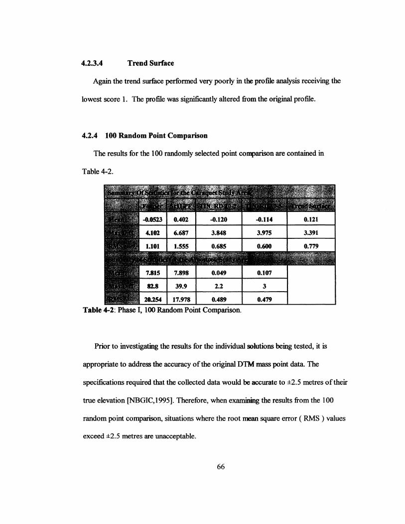
4.2.3.4 Trend Surface
Again the trend surface performed very poorly in the profile analysis receiving the
lowest score 1. The profile was significantly altered from the original profile.
4.2.4 100 Random Point Comparison
The results for the 100 randomly selected point comparison are contained in
Table 4-2.
39.9 2.2 3
17.978 0.489 0.479
Table 4-2: Phase I, 100 Random Point Comparison.
Prior to investigating the results for the individual solutions being tested, it is
appropriate to address the accuracy of the original DTM mass point data. The
specifications required that the collected data would be accurate to ±2.5 metres of their
true elevation [NBGIC,1995]. Therefore, when examining the results from the 100
random point comparison, situations where the root mean square error ( RMS ) values
exceed ±2.5 metres are unacceptable.
66
Further, it is useful to comment on the results from the I 00 randomly selected point
comparison. In general, the results are very good. However, in areas where elevation
changes rapidly over a short distance, the results are not as good. Where changes in local
relief are small, then the surface generated from the randomly generated points is very
similar to the original surface - which is desirable. However, where the relief rapidly
changes, the geometry of the random points can cause the two surfaces to differ and thus
they produce a higher RMS value. It is important to review the results of the I 00 random
point comparison with respect to the degree of relief change for the data set and triangle
geometry resulting :from the pattern generated by the random points.
While the comparison of elevation values between surfaces is a common method of
DTM accuracy assessment [Isaaconand Ripple, I990][Li,I99I] there are those who do
not agree with this method. In particular, Polidori et al. [I99I] suggest the use of fractal.
dimensions at different scales and orientations for the assessment ofDTM accmacy. It is
suggested that generation of an RMS error from random check points is not "sensitive to
interpolation artitacts ... and directional tendency [Polidori et al., I991] ". Certainly, the
research indicates that fractals may be used in detecting the presence of ridging, and
accuracy assessment. The research undertaken here will make use of the more classical
accuracy assessment technique of generating RMS values. Fractals are very useful in
assessing the quality ofDTMs without a reference surface. Further, since we are using
aspect as a detection method, the use of fractals is not necessary.
Scatter plots of the 100 random points comparing filtered and unfiltered elevations for
all the study sites are included in Appendix F.
67

4.2.4.1 LPF Spatial Filtering
Table 4-2 contains the results for comparing 100 randomly selected points between the
unfiltered SNB DTM and a LPF spatial fihered DTM. The results for Caraquet are
reasonable given the accuracy of the data. However, the results were very poor in the
Aroostook test site having the higher relief. Figure 4-5 illustrates a scatter plot for the
Aroostook study site.
Examination of the point where the maximum difference is located shows a small
localized peak(s) that was completely smoothed out by the averaging inherent in LPF
fihering. A resolution of 46 metres means that features that are smaller than 230 metres by
30 metres are subject to major degradation - particularly if the feature is a local maximum
or minimum.
AnloltDok5x1 LPF CCiftiPI'Isan
• • • •
• .... • • •
• • • • • •
• ••
200
~~~------~--------~--------~--------~-------, 200 2!il 1D
5x1LPF El_., tlhftll
Figure 4-5: Scatter Plot ofLPF v. Unfiltered Elevations, Aroostook, NB.
68

Figure 4-5 is a scatter plot that compares the elevations derived from LPF spatial
filtering and the unfiltered elevations for the same 100 randomly selected points. The plot
shows that, for the Aroostook study site, there is a strong linear correlation between the
elevation values except for those elevations where the filtered smoothed out the surfilce.
The linear correlation indicates that the elevation value for the points was similar between
the filtered and unfiltered DTMs. The points affected by the smoothing are shown as
outliers on the upper left hand portion of the graph. Results of this type are similar for all
the study sites.
4.2.4.2 Fourier Transformations
The Fourier techniques performed satisfuctorily in the Caraquet study site but did not
perform adequately in the Aroostook study site. Figure 4-6 illustrates comparison of
Fourier techniques for the Aroostook study site.
The resuhs demonstrate it was easier to separate the noise from the signal in the
Caraquet study site than in the Aroostook study site. Examination of the frequency
(magnitude) image for this study site demonstrated that this was indeed the case. Since
such a relatively large portion of the total DN value is noise (because there is low relief
relative to the magnitude of the ridging), only a small contribution to the DN value is
from elevation. This makes it simpler to pick out the noise.
When relief represents a larger contribution to the DN value, however, it is much more
69
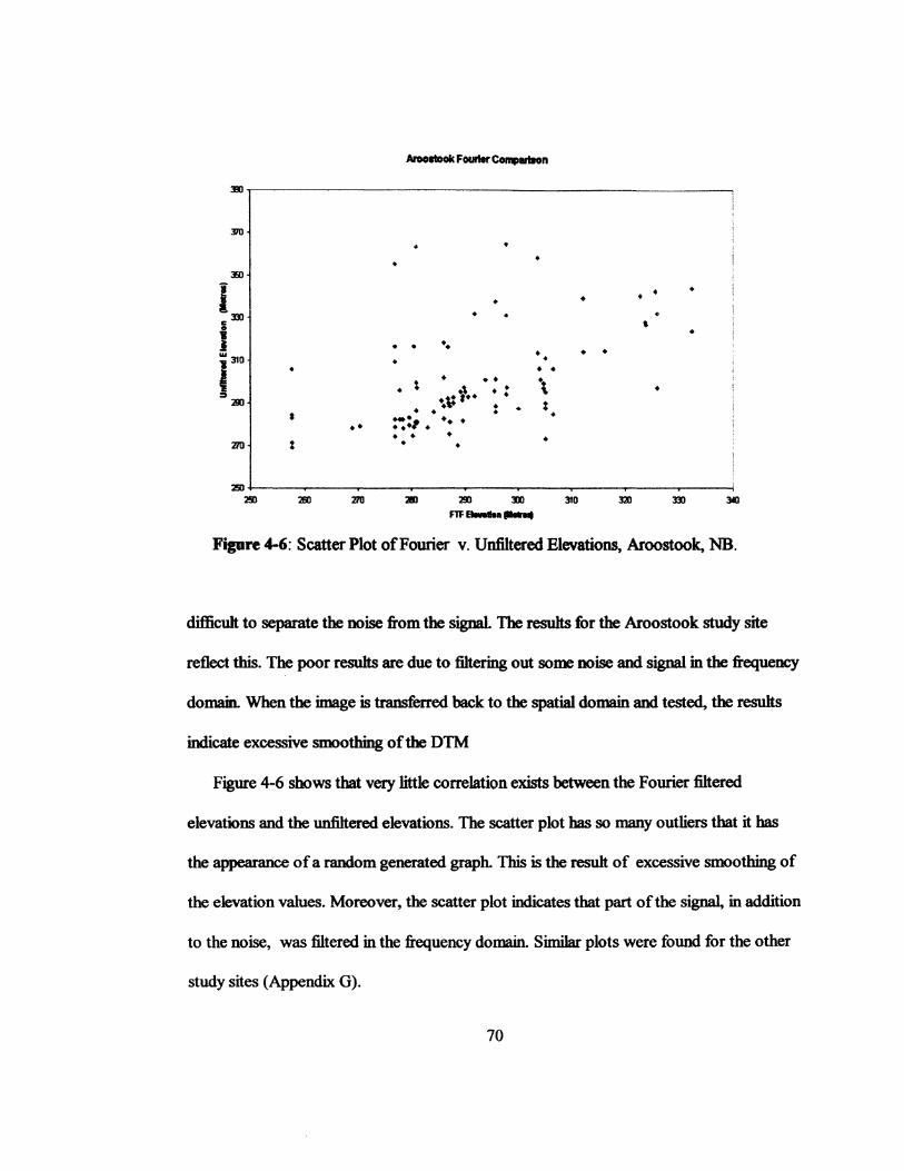
• • •
:sJ
• • • • •
• • • • • • • •• • •• • • • • • •• •t • ~ t\ • • • \t: , •• •
• • . : • • • ~:,. • • • ••
13Jl c • 1 ~~0 • ~
2!11
• • • • • • • 210 :
2!iO 2!iO 2111 311 ~0 Dl 3Jl 311
Figure 4-6: Scatter Plot ofFourier v. Unfiltered Elevations. Aroostook, NB.
difficult to separate the noise ftom the signal. The results for the Aroostook study site
reflect this. The poor results are due to filtering out some noise and signal in the ftequency
domain. When the image is transferred back to the spatial domain and tested, the results
indicate excessive smoothing of the DTM
Figure 4-6 shows that very little correlation exists between the Fourier filtered
elevations and the unfihered elevations. The scatter plot bas so many outliers that it bas
the appearance of a random generated graph. This is the resuh of excessive smoothing of
the elevation values. Moreover, the scatter plot indicates that part of the signal, in addition
to the noise, was filtered in the ftequency domain. Similar plots were found for the other
study sites (Appendix G).
70

4.2.4.3 TIN Random Densification
The results for the 1 00-point comparison of randomly-densified TINS are very
satisfactory for both study areas and both user defined parameters. In contrast to the other
solutions, TIN random densification actually performed better in the higher relief study
site. Examination of the data reveals no conclusive explanation of the better performance
in the Aroostook data.
However, it was found that the maximum differences occurred when the check point
falls in an area having a very steep slope. As a result, it is more difficult to interpolate an
accurate elevation value for the random point.
Figure 4-7 illustrates the scatter plot for the Caraquet study site. The plot exlubits a
positive linear correlation between the derived elevation values. This plot is representative
of the results achieved for all the study sites. For the most part, the outliers full in the
lower right hand quadrant of the graph. These outliers are caused by an increase in the
elevation interpolated during the TIN random densification process. A possible cause of
this is that the original point was a local minimum "pit") that was surrounded by higher
elevations~ when the point's elevation was is interpolated it is assigned a higher value.
71

Caraquet TIN Random o.nmc:atlon Compwtson • 2 Polnta per Original
10,--------------------------------------------
9
8
I I 7
i ... ... 6
I 5
• •
• • • •
•• ..
.,., .... ~· ... ~ .. ••• , ...
::;.. . . • • • • •
•
• •
• •• •
3+-------~----~------~------~------~------~----~ 3 5 6 7 8 9
Figure 4-7: Scatter Plot of TIN Random Densification v. Unfiltered Elevations, Caraquet, NB.
4.2.4.4 Trend Surface
10
The results for the trend surfilce are misleading. The performance in the 100 random
point comparison was deceivingly strong. The Caraquet study area is very flat and the
generalized surfilce is statistically close to the original data. This is reflected in these
results. However, it should not be forgotten that the trend surface completely breaks down
in area of significant relief Figure 4-8 illustrates the scatter plot for the Caraquet site
analysis. The scatter plot illustrates the lack of correlation between the surfaces.
72

C.-.qwl TNnd Swf8c;e COIIII*Inn
10
9
8
I . ~ ••• -<f, ): a . :.~,.· .. 1: 7 . .. . . : 0
l t w . ;.f l 6 • t ... . .. • ::0
5 •
•
3 ~ 5 6 7 8
T.- ..... a...........-Figure 4-8: Scatter Plot ofTrend Surface v. Unfiltered Elevations, Caraquet, NB.
4.2.5 Implications of the Results
• Spatial Filtering removes the detail of relief, therefore, shallow depressions such
as wetlands will be eradicated;
• The Fast Fourier Transform approach is dataset specific - each DTM dataset
must be evaluated and processed individually as opposed to a single "universal"
solution being applied on a jurisdiction-wide basis;
• The FFT approach is complex and may require specialized personnel to maximize
its potential;
73

• Smoothing of the detail (spatial filtering) may be the simplest option when
performing landscape rendering where loss of relief detail is not critical.
Examination of the resuhs of the 3-D visualization and profiles in Phase I clearly
demonstrates that the TIN Random Densification process and the Fourier filtering are
better solutions then either the Trend Surface or the Spatial Filtering. Examination of the
100 random point comparison revealed similar results. The TIN Random Densification
process has the two lowest RMS errors. Of particular note is the lower RMS error in the
Aroostook test patch which has a much higher relief The Fourier filter performed poorer
in this high relief test patch.
One concern arising out of discussions with SNB personnel was the effect of file size
by the various solutions.
Figure 4-9 illustrates the reJative file sizes in Arc View of the various filtering
techniques employed in Phase I. There is a dramatic increase in file size when add five
points per original point (ie. Aroo 1 0-5) as compared with only adding two points per
original point (ie. Arool0-2).
Reviewing the previous results indicates TIN Random Densification specifYing 5
points is only marginally superior to specifying 2 points. However, when file size is
considered, the TIN Random Densification approach specifying 2 points per original point
is superior to TIN Random Densification specifying 5 points per original point.
74

Relative DTM File Sizes 120 ----------------------------------------
100 ----------------------------------------
80 ---------------------------- --------- -----------------------------
60 ---------------------------- --------- -----------------------------
40
20
o~-----------------
Ale Size ( Klobyles )
CARAQUET STUDY SllE • UniBinld liN • liN R8ndom Denllllcdol1 2 Paints per Olglnal
• liN R..., O.lllalion 5 PalnCs per OiWnBI • R....- 0111- 48m Res. D 5x1LPF 1£] Fourier Fill8nld
• • AROOSTOOK STUDY SllE
• liN R..., O.illllcallun 5 Painbl per~ • RMIIrDlM· 48m RM .
• 5x1 LPF CJ Fourier Fltlrq
Figure 4-9: Re1ative File Sizes for Phase I.
4.2.6 Phase I Analysis Decisions and Diseussion
The following is a list of conclusions and recommendations to carry into phase II.
• The results of phase I analysis demonstrate that TIN Random Densification -
specifying 2 points per original point -produced the best results based on the
75

criteria specified for Phase I;
• By its very random nature, any DTM processed by TIN Random Densification is a
unique solution, that is to say if the same DTM was reprocessed, a slightly
different result would be obtained;
• The results from the Fourier filtering were not as good as was expected in
comparison to results obtained by other researchers as described in the
background literature;
• Fourier filtering is more complex than the other solutions and warrants carryover
to Phase II in order to fully explore its possibilities.
4.3 Phase ll Results
Phase II of the testing saw the reintroduction of the Hayesville test site. In addition,
the use of the 1 kmx 1 Ian test patches were abandoned in mvour of testing solutions on
full map sheets.
Only the TIN Random densification and Fourier filtering solutions were tested in this
phase. All the other proposed solutions performed so unsatistactorily in Phase I testing
that it was decided that they didn't warrant carryover into Phase II. Further, under this
writer's direction, Fourier :filtering solutions were performed on the three test sites by
CTM Inc., Boulder Colorado, as part of a pilot study. The criteria of comparison
76

employed in this phase included: contouring, 100 random point comparison, and
hydrological analysis.
4.3.1 Contouring
Contours were generated for each map sheet in each of the three study areas. Plots of
the generated contours are attached as Appendix G. Moreover, for each study area,
contours generated from the unfiltered and filtered data sets were compared in order to
ascertain whether the ridging (which is readily detected when a contaminated dataset is
contoured) can be detected when the filtered DTM is contoured. Figure 4-10 illustrates a
small contoured portion of a contaminated DTM. The ridging is retlected in the
contouring by the long narrow parallel contour lines. Figure 4-11 represents a contoured
DTM filtered using the TIN Random Densification Process. Clearly, the pattern of the
ridging is diminished in the DTM filtered using the TIN Random Densification process.
Figure 4-10. Caraquet, O.Sm Contours from Unfiltered TIN.
77

Figure 4-11: Caraquet, 0.5m Contours from TIN processed with TIN Random Densification.
Figure 4-12. Caraquet ,0.5m Contours from CTM Fourier Filtering.
78

Figure 4-12 illustrates contours derived for the same area as shown above :from the DTM
created by Computer Terrain Mapping (CTM) using their Fourier filtering technique. The
results indicate that significant smoothing of the data has taken place. Undeniably, the
ridging has been removed and the contours are more aesthetically pleasing than those
contours in the previous two figures. However, since the extent of the smoothing is a
concern, the 100 point comparison was also performed on the CTM filtered image in an
attempt to quantify the overall "distortion" of the modified DTM' s.
The results :from the contouring analysis are summarized in Table 4-3. The individual
results of the contouring are assessed on a scale of"1" to "5". A score of"5" indicates
that the generated contours contain no remaining trace of the ridging. A score of"1"
indicates that the ridging still remains in the contoured image.
Caraquet: Unfiltered 1
Caraquet: TIN_RD 10-2 3
Caraquet: Fourier - CTM 5
Aroostook: Unfiltered 2
Aroostook: TIN RD 10-2 3
Aroostook: Fourier - CTM 5
Hayesville: Unfiltered 1
Hayesville: TIN_RD 10-2 3
Table 4-3: Sununary of Contouring Analysis.
The contours generated by Computer Terrain Mapping's Fourier techniques scored
the best results for all the study sites. In general, the contours for CTM's filtered DTMs
79

showed little or no trace of ridging and they also bad an aesthetically pleasing shape.
Contrasting this are the contours generated :from the randomly densified DTM. These
contours definitely show a reduction in ridging but, they have an unpleasing angular
quality to them. Certainly, a thinning or, contour generalization program should be used to
produce a better contour map.
4.3.2 100 Random Point Comparison
The data sets processed by CTM were analysed and compared with TIN Random
Densification process by comparing interpolated values for the same 100 randomly
selected points used in the previous analysis.
0.185 0.149
3.9 4.9 6.7
0.730 1.114 1.525
Table 4-4: Phase II, 100 Random Point Comparison.
Table 4-4 shows the resuhs of this investigation. The results of the 100 random point
80

comparison show that the images filtered by Computer Terrain Mapping {CTM) have
higher RMS errors in test sites having higher relief than the results achieved using TIN
Random Densification. These results are due to excessive smoothing by the process used
byCTM.
• Random PointS Percent Slope
-<~ -7%-141J6 -141J6-211J(, ->281J6
Figure 4-13: Slope based 100 Random Point Comparison, Aroostoo~ NB.
81

14.9 11.000 18.1 10.500
4.439 6.073 9.407 0.849
Table 4-5: Phase ll: Slope Based 100 Random Point Comparison.
The results in Table 4-4 indicated that the performance of the TIN random
densification and CTMs Fourier techniques were affected by the relief: To investigate this,
statistics were generated for 100 randomly selected points that were classified by its
surrounding slope, as illustrated in Figure 4-13. Table 4-5 shows the resuhs ofthis
investigation.
The slope based analysis shows that the amount of smoothing, as indicated by the
maximwn difference, increases with slope, for DTMs processed by CTMs Fourier
techniques. Moreover, the RMS error generally increased with slope for these DTMs. No
82

such conclusion can be drawn for DTMs processed by TIN Random Densification. The
statistics show a random pattern in the statistical measure over the range of slope classes.
4.3.3 Hydrological Analysis
Caraqu,~t Stu~.~~-L .... -·-·"' .. .. ... ~!Sfook S~dy Area ~!~~~~-~--. ~!!~.ct~EI!ISir!llll ~~~ '[If_~~~~ .. -~ •CM!i ~·c.~~
1East 281 . f~ ~Ll.~~-- .. p .!.\~·.: --~---=1rii·1~5% -... 4 Scdh -1003
16:west ! 841. t5:West .m-t.l'f. ·--_ij;~·-·:::.:.~~1~!~ti~: :·.::·· . .. -~64iibth ..... ·:em: . ······ ..
Table 4-6. Summary of Hydrological Analysis.
H~lle Study Aria ........... "' _ . _Chqe~#ttflwyt~~"ti[IJIitctian CMii [lfiaCe!f "~
J_;fa&1__ ·--~. ···--·-4Scah -ltl:-1.1'11 .
. ~ . . .
.. J6.~ -~1114 ____________ .
. . ~Ukd . :4:lf ~~---...
The resuhs of the hydrological analysis are summarized in Table 4-6. The Table shows
the resuhs of the hydrological analysis for the three study sites. The upper half of the table
is for the DTM' s that were filtered using TIN Random Densification. The lower half is for
those DTMs processed in the pilot study with CTM Inc.'s Fourier techniques. For each
study site and filtering method, the difference in the number of cells representing streams
was calculated between the unfiltered and filtered DTM. The table has columns for the
cardinal direction (Cardinal), difference in the number of cells representing streams (Diff
of Cell), and the percentage change for the total number of cells. The rows that are in bold
indicate the cardinal direction along which the mass point profiles were collected. These
83

are the values of greatest interest as a good filtering process will reduce the number of
streams running along the troughs between the ridges.
The results of the hydrological analysis demonstrate that, in general, only TIN Random
Densification reduced the number of cells representing streams running in the same
direction as the original mass point profile lines. CTM's Fourier filtering actually increased
the number of generated phantom streams in all except one case. It is important to note
that, in the Aroostook study area, we are interested in the reduction of cells representing
streams in the east/west directions because the original mass point profile lines also run in
the east/west directions. The final generated stream network coverages may be found in
Appendix I.
4.3.4 Phase II Analysis Decisions and Discussion
The following represent the decisions and recommendations for the analysis carried
out in Phase II.
• Any contamination of a DTM by ridging will bias automatically generated stream
paths.
• Fourier Filtering techniques and TIN Random Densification both have the
advantage of minimal alteration of the original data, or restoration of the
original data, as opposed to spatial filtering or trend surfaces which degrade the
detail of relief
84

• Fourier Filtering has been implemented commercially which reflects the
complexity of this solution.
• TIN Random Densification DTMs can produce contours with a "jagged"
appearance, which may cause another concern with user groups. These contours
could be smoothed to produce more realistic results.
• TIN Random Densification DTMs have larger file sizes than the original
unfiltered datasets.
4.4 Implementation Considerations
Where legacy data is contaminated by the ridging phenomena, fihering solutions may
be implemented in three ways: project by project basis, as required basis, or on a program
basis.
Implementation on a project by project basis means that the agency in charge of the
legacy datasets informs its users of alternative solutions and provides a list of consultant's
having the expertise to commercially perform ridging fihering services. Once provided
with this information, users are then left to solve their own ridging problems
The agency in charge of the contaminated DTMs may opt to provide an executable
program in which users could acquire. Users would then install and use the programs to
filtered their contaminated DTMs. If TIN Random Densification is implemented in this
"as- required" basis, then users must be told to expect slightly different resuhs with each
85
filtered DTM. Moreover, users may encounter problems when comparing results with
others filtering the same DTM using TIN Random Densification. The major benefit of
these first two options is the lowcost of implementation.
The final implementation scheme is to take a program based approach. This is the most
expensive implementation solution. In this scenario, TIN Random Densification ( or what
ever solution is utilized ) is used to process all the DTMs for a particular jurisdiction such
as province or state. The benefits of a program based approach are increased user
confidence and sense of goodwill in the agency and its datasets. Further, tighter quality
control procedures will produce more consistent resuhs.
4.5 Chapter Summary
Based on the testing criteria in the two phases of testing, TIN Random Densification
had the best performance as a method of removal of the ridging effect from SNB DTM
files. Fourier filtering had the second best performance in the testing.
The primary strengths of TIN Random Densification are that it is a ''reorganization" of
the original data rather than a smoothing filter. In addition, TIN Random Densification is
unaffected by the degree of relief in the file and it is a "batch" filtering operation.
The weaknesses inherent in TIN Random Densification are that it produces unique
solutions with each implementation, generates poor contours and increases file size.
TIN Random Densification, or any other solution to the ridging effect, may be
implemented in three ways: project by project basis, as required basis, or on a program
basis.
86
5
CONCLUSIONS
The final chapter of this report will review and summarize the work done herein. First
the project objectives and the analysis approach will be reviewed. Next, the results from
the two phases of testing will be summarized. In particuJar, the testing results from TIN
Random Densification and those obtained from a pilot study with Computer Terrain
Mapping Inc. will be discussed. Based on the analysis performed in this report, the best
solution to minimize the ridging phenomena in SNB D1M datasets will be presented.
Finally, areas for future research and concluding remarks will be given.
5.1 Review of Project Objectives
The objective of this research was to :find the cause and a method of removal for the
ridging effect from Service New Brunswick DTM files. To accomplish this a number of
secondary objectives were studied. These included:
(1) To establish the magnitude of "ridges" and to identify a testing criterion for the
removal of ridging from DTM data. Four testing criteria were developed, as
described in Chapter 3, to provide a foundation for the analysis of solutions to the
ridging effect.
87

(2) To test procedures to automatically identify the existence "ridges" within
datasets. Chapter 3 outlined the investigation into the automatic detection of
ridging and the results of this work were presented in Chapter 4.
(3) To test several alternative compensation procedures to remove or, diminish the
ridging effect. Chapter 2 outlines the background research used to determine four
compensation procedures. Chapter 3 descn"bes the testing design and approach for
the proposed compensation procedures. Chapter 4 presents the result obtained,
over two phases of testing, of the proposed compensation procedures.
(4) Malee a recommendation on the most appropriate method of removal of the
ridging and to explore strategies for implementation of the necessary changes to
the DTM data files. Based on the results :from the testing, the most appropriate
removal method was identified and suggestions were made towards its
implementation.
The report was structured in the following manner. Chapter 1 provided the context
and summarizes the problem of ridging in SNB DTM datasets. The principal objective of
the research is stated and secondary objectives were also described. In addition, the
significance of the research is described. A summary of the proposed approach is
presented along with the constraints of the project.
Chapter 2 summarized the relevant background research including the cause of
88

ridging. In particular, various filtering methods were explored. These included; simple low
pass filtering techniques, Fourier transform filtering, TIN Random densification and trend
surfaces.
Chapter 3 contained descriptions of the testing procedures to detect ridging, and the
testing criteria for contaminated SNB DTM data. In particular, attention was paid to
indicating practical improvements to the data sets. Further, based on the improvement
criteria, various approaches to eliminate or, reduce ridging were discussed.
Chapter 4 contained the summary of analysis, discussion and results obtained in the
investigation undertaken in the previous chapters. In particular, the implications of the
resuhs, analysis decisions and recommendations were presented for the two phases of
testing. Chapter 4 a1so describes the inclusion of a small pilot project with Computer
Terrain Mapping, Boulder Co., who provided a Fourier technique to filter out ridging
primarily for USGS Level-l DEMS.
5.2 SUJDJDary of Testing Results
The testing was broken up into two phases. The first phase was designed to quickly
eliminate proposed solutions whose performance clearly was unsatis:fuctory based on the
testing criteria. The second phase of testing was undertaken to focus on the solutions
whose performance in early testing indicate that they may possibly exh.J.bit the best overall
performance based on the criteria of improvement. Conclusions on the best solution to the
ridging effect will a1so be presented.
89

5.2.1 Phase I Testing Results
The four proposed solutions: LPF spatial filtering, Fourier transformation techniques,
TIN Random Densification, and Trend surfitce generation were tested against three
criteria of improvement. These criteria were: 3-Dim.ensional visualization, profile analysis,
and 100 randomly generated point comparison. In addition, concerns raised by SNB
personnel on the file sizes of the filtered DTMs were addressed. In addition, the testing
was performed using a histogram of aspect values to detect ridging.
The testing revealed that the use of histogram of aspect value of a DTM to detect the
presence of ridging is not a suitable detection method for most types of terrain. While the
results were good for area having low relief: the method fiilled in test sites with more
variable terrain. The fiillure is due to the inability of the histogram to detect the
proportionally smaller contnbution of ridging to the DN values of the DTM and thus the
contribution to aspect.
Filtering solutions based on LPF spatial filtering, Fourier filtering techniques, and trend
surfuce generation performed poorly with respect to the testing criteria for Phase I.
However, software limitations and perhaps user inexperience contributed to the poor
perfonnance of the intriguing Fourier filtering approach. As a resuh, TIN Random
Densification and Fourier filtering techniques were carried over into the second phase of
the testing. LPF spatial filtering, and trend surface generation were not carried over into
the second phase oftesting.
90

5.2.2 Phase ll Testing Results
TIN Random densification and CTM's Fourier filtering techniques performance were
tested against three criteria: contouring, 100 random point comparison, and hydrological
modelling. CTM's solution produced better contours than did TIN Random densification.
However, the contours produced by TIN Random densification were an improvement
over those derived :from the contaminated datasets.
TIN Random Densification showed better performance in the hydrological modelling.
DTMs generated :from randomly densified datasets showed a greater percentage reduction
in the creation of phantom streams than DTMs processed using CTM's Fourier
techniques.
In the 100 random point comparison criteria, TIN random densification performed
better than CTM's solution. Further, the statistics show that significant smoothing results
:from CTM' s Fourier solution. Moreover, breaking down the results of 100 random point
comparison based on slope demonstrated that CTM's solution performed poorly in areas
of higher slope. No such trend was discovered for TIN Random Densification.
Therefore, based on the results for both phases of testing, and in particular giving a
greater weighting to visualization and statistical performance, the most appropriate
method of removal for the ridging efrect :from Service New Brunswick DTM files is TIN
Random Densification followed closely by Fourier filtering as a viable alternative.
91

5.3 Future Research
The research performed in this report has suggests that future areas of research could
include:
• TIN Random Densification has been implemented in this report as a " proof of
concept" only, and any industrial implementation will require several improvements.
For Example: (a) implement the algorithm in a lower level programming language ( i.e.
C) to increase processing speed; (b) address the addition ofbrealdine data; (c) mask
or clip any densified points that fiill within water bodies: and (d) set a minimal
proximity tolerance for all points ( ie no two points shall be closer than X metres
apart), to name a few.
• Any useful implementation will require the investigation of edgematching issues
among randomly densified DTMs. Once a more robust algorithm is produced, it would
be beneficial to undertake a small pilot study to investigate just how adjacent fihered
DTMs would behave. Further, methods must be developed to edgematch adjoining
randomly densified DTMs.
• Any solution should be examined in light of a cost benefit analysis. Given that some
degradation of the data occurs no matter what filtering solution is used, what are the
benefits and costs associated with filtering DTM datasets. In short, is it a worthwhile
endeavour?
92

5.4 Concluding Remarks
No solution to the ridging phenomena will remove all remnants of the ridging. This
research addressed the problem from a data visualization point of view by creating a
solution based TIN Random Densification. However, the data visualization point of view
suggests that the cause of the ridging phenomena is the original method of mass point data
collection. Collection of mass point data along parallel profile lines is seen as fimdamental
cause of ridging by supporters of this view of the problem. Any DTM filtered or not, that
is derived from data collected in this manner is contaminated with ridging. At some point,
consideration must be given to discarding this data and recollecting it using a better
method.
The resuhs of this report have demonstrated that TIN Random Densification is the
best technique, followed closely by Fourier Filtering as a viable alternative.
93

References
Berry, J. (1998). ''Unlock the Statistical Keystone", Beyond Mapping, GeoWorld, Vol 9, No. 11, November, pp.28-29.
Bonham-Carter, G. (1994). Geographic Information Systems for Geoscientists: Modelling with GIS, Pergamon, New York.
Brown, D. and T. Bara, (1994). "Recognition and Reduction of Systematic Error in Elevation and Derivative Surfilces from 7112-Minute DEMs." Photogrammetric Engineering and Remote Sensing, Vol. 60, No.2. February, pp. 189- 194.
Brunson, E.B. and R. W. Olsen (1980). ''Data Digital Elevation Model Collection Systems." Proceedings of the Digital Te"ain Models Symposium, American Society ofPhotogrammetry, St. Louis, Missouri, 9-11 May, pp. 72 - 98.
Coleman, D.J. (1998). Personnel Communication. Chairman, Dept. Geodesy and Geomatics Engineering, University ofNew Brunswick, June.
Cowie, F. (1998). Personnel Communication. Director, Atlantic Salmon Museum, Doaktown, New Brunswick, June.
ESRI (1997). ''Using the Arc View Spatial Analyst, Version 1.1.", Publication of Environmental Systems Research Institute, pp 90-93.
Fredrikson, P. (1980). ''Terrain Analysis and Accuracy Prediction by Means ofthe Fourier Transformation." Proceedings ISP Congress, Comm. IV, Vol. XXIII, Part B4, pp.284-293.
Garbrecht J. and P. Starks (1995). "Note on the Use ofUSGS Levell 7.5-Minute DEM Coverages for Landscape Drainage Analyses." Photogrammetric Engineering and Remote Sensing, Vol61, No. 5. May, pp 519-522.
Hassan, M. (1988). "Filtering Digital Profile Observations." Photogrammetric Engineering and Remote Sensing, Vol.54, No.10, October, 1391-1394.
Isaacson D. and W. Ripple (1990). "Comparison of7.5 Minute and 1-Degree Digital Elevation Models." Photogrammetric Engineering & Remote Sensing, Vol.56, No.ll. November, pp 1523-1527.
Leblon, B. (1997). "Ch V. Spatial Filtering." Class notes for FOR4305, Faculty Forestry and Environmental Management, University ofNew Brunswick.
94

Lee, Y.C. (1998). Personnel Communication. Professor, Dept. Geodesy and Geomatics Engineering, University ofNew Brunswick, July.
Leese, M (1998). Personnel Communication. Computer Systems Manager, Ocean Mapping Group, Dept. Geodesy and Geomatics Engineering, University ofNew Brunswick, November.
Li, Z. (1991). "Effects of Check Points on the Reliability ofDTM Accuracy Estimates Obtained from Experimental Tests." Photogrammetric Engineering & Remote Sensing, Vol.57, No. 10, October, pp. 1330-1340.
Lillesand, T and R. Kiefer (1994). Remote Sensing and Image Interpretation 3rt1 Edition, John Wdey and Sons, New York.
Makarovic, B. (1975 ). "Amended Strategy for Progressive Sampling." The fl'C- Journal 1975- 1.
Miller, C.L. and R.A. LaFlamme (1958). ''The Digital Terrain Model- Theory & Application." Photogrammetric Engineering and Remote Sensing, Vol. 24, No.3, June, pp. 433- 442.
NBGIC, (1995). ''User Guide to The Digital Terrain Model Database." New Brunswick Geographic Information Corporation, Fredericton, New Brunswick.
Pan, J. (1989). "Spectral Analysis and Filtering Techniques in Digital Spatial Processing." Photogrammetric Engineering and Remote Sensing, Vol.55, No. 8, 1989, pp. 1203-1207.
PCI Inc. (1997). ''Using PCI Software", VeiSion 6.2, PublicationofPCI Inc., November.
Polidori L., J. Chorowicz and R. Guillande (1991). "Description of Terrain as a Fractal SurfBce, and Application to Digital Elevation Model Quality Assessment." Photogrammetric Engineering and Remote Sensing, Vol. 57, No.10, October 1991,pp. 1329-1332.
Pearson, M. (1998). Personnel Communication. CEO and Director ofMarketing, GeoNet Technologies Inc., August.
Pegler K.H., and D.J. Coleman (1998)."Removal of the Ridging Effect from New Brunswick Digital Terrain Model Data" Contract proposal prepared by the Dept. ofGeomatics Engineering, Laboratory for Geographical Engineering, University of New Brunswick, Fredericton, N.B., Canada, for Service New Brunswick, Fredericton N.B., July, 7 pp.
95

Russell, E., M. Kumler and H. Ochis, (1995). "Identifying and Removing Systematic Errors on USGS DEMs, GIS in the Rockies Conference Proceedings, Denver, CO (Sept 25-27, 1995).
Russell, E. and H. Ochis, (1996). "Mitigation Methods for Systematic Errors in USGS DEMs." White Paper, Computer Terrain Mapping, Inc. Boulder Colorado.
Schowengerdt, R.A. (1997). Remote Sensing, Models and Methods for Image Processing. 2nd ed., Academic Press, MA.
96

Bibliography
Carnahan, W. and Zhou, G. (1986). "Fourier Transform Techniques for the Evaluation of Thematic Mapper Line Spread Function." Photogrammetric Engineering and Remote Sensing, Vol. 52, No.5, May, pp. 639-648.
Crippen, R.E. (1989). "A simple Spatial Filtering Routine for the Cosmetic Removal of Scan -Line Noise from Landsat TM P-Tape Imagery." Photogrammetric Engineering and Remote Sensing, Vol. 55, No.3, March, pp. 327-331
Hoffi:nan, F. ( 1998 ). "An Introduction to Fourier Theory." http://aurora.phys.utk.edu/-forrest/paperslfourier/index.html, August 20.
Makarovic, B. (1975 ). "Amended Strategy for Progressive Sampling." The lTC- Journal 1975- 1.
Pan, J. and C. Chang (1992). "Destriping ofLandsat MSS Images by Filtering Techniques." Photogrammetric Engineering and Remote Sensing, Vol.58 No.1 0, October 1992, pp. 1417-1423.
Thapa, K. and J. Bossler, (1992). "Accuracy of Spatial Data Used in Geographic Information Systems." Photogrammetric Engineering & Remote Sensing, Vol. 58, No.6, June. pp 835-841.
Walsh, S.J., D.R. Lightfoot and D.R. Butler. (1987). "Recognition and Assessment of Error in Geographic Information Systems." Photogrammetric Engineering and Remote Sensing, Vol, 53, No. 10, October, pp. 1423-1430.
Whitestar Ltd. (1998). "Digital Elevation Data." http://www.whitestar.com/ded.html, 29 July.
97

APPENDIX A
A venue Script: Ridge_ Detector .ave
98

~>>>>>>>>>>>>>>>>>>>>>>>>>>>>>>>>>>>>>>>>>
1 Ridge_ Detector 1 A simple script to detect the occurance of 1 "Ridging" in a data set utilizing the 1 % of a TINs Aspect
1 January 16, 1999 1 By: Kevin H. Pegler
1 Requires that the TIN theme in question 1 to be the active document
~>>>>>>>>>>>>>>>>>>>>>>>>>>>>>>>>>>>>>>>>>
1 Get the active TIN document
1 Inform the user that the TIN theme 1 must be the first theme in TOC
AnswerChar = MsgBox. YesNo ( "Is the TIN Theme first in the TOC & is it Active ?","Warning!", True)
if ( AnswerChar = False ) then Exit
end
1 get the user defined tolerance tolerance= MsgBox.lnput ("Input as a decimal value","User defined% ofParallel TIN Facets Representing Ridging", "0.52") ~>>>>>>>>>>>>>>>>>>>>>>>>>>>>>>>>>>>>>>>
1 Convert the TIN to an aspect GRID
1 including => Spatial.Aspect
1 Spatial.Aspect
the View= av.GetActiveDoc
1 get active theme t = theView.GetActiveThemes.Get(O)
' tum grid or tin into slope grid
99

if (t.GetClass.GetClassName = "GTheme") then g = t.GetGrid r = g.Aspect
elseif(t.GetCJass.GetClassName = "STheme") then theTin = t.GetSurface box= Rect.Make(0@0,1@1) cellSize = 1 ce = AnalysisPropertiesDialog.Show(theView,TRUE,"Output Grid Specification") if(ce =NIL) then
return NIL end ce. GetExtent(box) ce. GetCellSize( cellSize) r = theTin.AspectAsGrid( cellSize,box)
else return NIL
end
1 set name of data set, triggers evaluation aspectFN = av.GetProject.GetWorkDir.Mak.eTmp("aspct", "") r.Rename( aspectFN)
1 check to see if output is valid if(r.HasError) then
return NIL end
1 create a theme gthm = GTheme.Mak.e(r)
1 create appropriate legend for theme theLegend = gthm.GetLegend theLegend.Interval(gtbm, "Value" ,9) flatCo1or = Color.Mak.e flatColor.SetRgbList( { 175,175, 175}) nColor = Color.Mak.e nColor.SetRgbList( {255,0,0}) neColor = Color.Mak.e neColor.SetRgbList( {255, 165,0}) eColor = Color.Mak.e eColor.SetRgbList( {255,255,0}) seColor = Color.Mak.e seColor.SetRgbList( { 0,25 5,0})
100

sColor = Color.Make sColor.SetRgbList( {0,255,255}) swColor = Color.Make swColor.SetRgbList( {0,165,255}) wColor = Color.Make wColor .SetRgbList( { 0,0,255}) nwColor = Color.Make nwColor.SetRgbList( {255,0,255}) labelList ={"Flat (-1)","North (0-22.5,337.5-360)",''Northeast (22.5-67.5)","East (67.5-112.5)",''Southeast (112.5-157.5)",''South (157.5-202.5)","Southwest (202.5-247.5)",''West (247.5-292.5)","Northwest (292.5-337.5)"} rangeList = {"-1 ",''0- 22.5,337.5- 360",''22.5- 67.5",''67.5- 112.5",''112.5-157.5","157.5- 202.5","202.5- 247.5","247.5- 292.5","292.5- 337.5"} theColorList = {flatColor,nColor,neColor,eColor,seColor,sColor,swColor,wColor,nwColor} theLegendCJasses = theLegend.GetClassifications count= 0 for each c in theLegendClasses
c.SetLabel(JabelList.Get( count)) c.SetRangeString(rangeList.Get( count)) count = count + 1 if (count > 8) then break
end end theLegendSymbols = theLegend.GetSymbols count= 0 for each s in theLegendSymbols
s.SetColor(theColorList.Get(count)) count = count + 1 if (count > 8) then
break end
end gthm.UpdateLegend
' set name for theme gthm.SetName("Aspect of"+ t.GetName)
' add theme to the View theView.AddTheme(gthm) ~>>>>>>>>>>>>>>>>>>>>>>>>>>>>>
101

'make the aspect theme the active doc etc.
thecurrentThemes = theView.GetThemes thecurrentThemes.Get(O).SetActive (True) thecurrentThemes.Get(O).SetVisible (True) thecurrentThemes.Get(l).SetActive ( FaJse) thecurrentThemes.Get(l).SetVisible ( FaJse) theView.lnvalidateTOC(nil)
~>>>>>>>>>>>>>>>>>>>>>>>>>>>>>>>>>>>>>>>>>>>>>>>>>>>>>>>>>>
' histogram of the for the aspect data
' Spatial.Histogram
the View= av.GetActiveDoc
' create histogram for each active GTheme for each tin theView.GetActiveThemes
if (t.ls(GTIIEME).Not) then continue end
I apply mask theMaskGTheme = theView.GetExtension(AnalysisEnvironment).GetMask if (theMaskGTheme =NIL) then
valueTheme = t else
valueGrid = t.GetGrid.ExtractByMask(theMaskGTheme.GetGrid) value Theme = GTheme.Make(valueGrid) if (valueGrid.HasError) then
return NIL end valueTheme.SetLegend(t.GetLegend) valueTheme.SetName(t.GetName)
end
' create histogram if (the View.GetGraphics.HasSelected) then
if(theMaskGTheme =NIL) then theChart = valueTheme.Histogram(TRUE, NIL, TRUE)
else theView.AddTheme(valueTheme)
102
theChart = valueTheme.Histogram(TRUE, NIL, TRUE)
theView.DeleteTheme(valueTheme) end theChart.SetName("Histogram of"+ t.GetName +"Within Selected Graphics")
else theChart = valueTheme.Histogram(TRUE, NIL, FALSE) theChart.SetName("Histogram of" + t.GetName)
end
' set chart properties theChartDisplay = theChart.GetChartDisplay theChartDisplay.SetGroupGap(O) theChart.GetWm.Activate
end
~>>>>>>>>>>>>>>>>>>>>>>>>>>>>>>
tstVtab = theChart.GetVtab
nwnrecs = tstVtab.GetNumRecords
~>>>>>>>>>>>>>>>>>>>>>>>>>>>>>>
cntr= 0
theClassList = List.make
theCountList = List.make
theCiassLabelList = List.make
for each record in tstVtab
countField = tstVtab.FindField ( "Count" )
subcntr = tstVtab.ReturnValue ( countField, record)
103

cntr = cntr + subcntr
classField = tstVtab.FindField ("Class")
theClassList.Add ( tstVtab.ReturnValue ( classField, record))
theCountList.Add ( tstVtab.ReturnValue ( countField, record))
Class_labeField = tstVtab.FindField ( "Class_labe")
theClassLabelList.Add ( tstVtab.ReturnValue ( Class_labeField, record))
end
~>>>>>>>>>>>>>>>>>>>>>>>>>>>>>>>>>>>>>>>>>>>>>>>>>>>>
'Loop through the lists and test for ridging
i= 1
while(i<S)
theRidgeNum = theCountList.Get(i) + theCountList.Get(i + 4 )
thePercntRidgNum = theRidgeNum/cntr
if (thePercntRidgNum > tolerance.AsNumber ) then
MsgStr = "The ridging is running: " + theClassLabelList.Get(i) ++ theClassLabelList.Get(i + 4)
MsgBox.Info ( MsgStr, "Ridging Present!") Exit
end i=i + 1
end
104

APPENDIXB
Avenue Script: TIN_RD.ave
105

~>>>>>>>>>>>>>>>>>>>>>>>>>>>>>>>>>>>>>>>>>
'TIN Random Densifier : TIN RD.ave 'By Kevin Pegler. Decl2,1998
'>>>>>>>>>>>>>>>>>>>>>>>>>>>>>>>>>>>>>>>>>
the View= av.GetActiveDoc for each tin theView.GetThemes
if(t.lsVisible) then t.SetVisible(F ALSE) end
end '#Hff#N#If#lf#####lll#l##ffff#JUI#IH/ff#Jflfi!#Nif#IUf/f##f/ffllflfllfll#fiJ#UNIII 'Dec 22 '98 'Create a automatic random point graphic generator 'msgBox.Info ("Auto Random Point Generator", "Info")
theThemes=theView.GetThemes
' Make the first theme active
ptFfheme = theThemes.Get(O) ptFfheme.SetActive( TRUE ) ptFTheme.SetVisible ( TRUE )
•••••••••••••••••••••••••••••••••• 'get user inputs
labels = { "number of points to add per point", "minimum distance" } defaults= { "2", "10" } user List = MsgBox.Multilnput( "User Input", "TIN_ RD", labels, defaults ) 'MsgBox.ListAsString( order, "Here is your order", "LOOK")
Npoints = userList.Get( 0 ).AsNumber Mindist = userList.Get( I ).AsNumber
••••••••••••••••••••••••••••••••••••
106

'get the max min coords for the selected theme
boundingRect = ptFfheme.ReturnExtent
minBigXNum = boundingRect.GetLeft minBigYNum= boundingRect.GetBottom
maxBigXNum = boundingRect.GetRight maxBig YNum =boundingRect.GetTop
ptfeaturesToCheck = ptFfheme.GetFTab total =ptFfheme.GetFTab.GetNumR.ecords
'setup a decent symbol size
'%%%%%%%%%%%%%%%%%%%%%%%%%%%%%%%%%%%%% 'top o the looper for each point in the theme
X_ coord.Field = ptfeaturesToCheck.Find.Field ("X_ coord") Y _ coord.Field = ptfeaturesToCheck.Find.Field ("Y _ coord") for each rec in ptfeaturesToCheck
currentXNum = ptFTheme.GetFTab.ReturnValue( X_coord.Field, rec) currentYNum = ptFTheme.GetFTab.ReturnValue( Y_coord.Field, rec)
'create the local 35m kernal around the current point
kerna1MinXNum = currentXNum- 35
kernalMinYNum = currentYNum- 35
kernalMaxXNum = currentXNum + 35
kernaJMaxYNum = currentYNum + 35
'test the kernal values
if ( kerna1MinXNum< minBigXNum) then kernaJMinXNum = minBigXNum
end if ( kernaJMin YNum <minBig YNum) then
kernalMinYNum = minBigYNum
107

end if ( kemalMaxXNum >maxBigXNum) then
kemalMaxXNum = maxBigXNum end if( kemaiMaxYNum>maxBigYNum) then
kemalMaxYNum = maxBigYNum end
randptCounter = 1
'********************************* while (randptcounter < Npoints) 'puts n points into each point's kernal
XcoordNum = Number.MakeRandom( kernalMinXNum, kernaiMaxXNum) Y coordNum = Number.MakeRandom( kemalMinYNum, kemaJMaxYNum) distNum = ( (XcoordNum- currentXNum)A2 + (YcoordNum- currentYNum)A2 ).Sqrt
if ( distNum > Mindist ) then thePoint = Point.Make(XcoordNum, Y coordNum) theGShape = GraphicShape.Make ( thePoint ) theView.GetGraphics.Add (theGShape) the View .Invalidate randptCounter = randptCounter + 1
end end 'botton of randpt loop ••••••••••••••••••••••••••••••••••
end 'bottom of the pointlooper '%%%%%%%%%%%%%%%%%%%%%%%%%%%%%%%%%%%%% '#fflflflflff/fllf#lflf {f!U/fflfflfffWiffllllffJII fllf/NIIW#Iff!IN/1/fl f/lflf#f/11 fflff/1/#fffiH!/
'Graphic.SelectAll theDoc=av.GetActiveDoc theDoc.GetGraphics.SelectAll
msgBox.Info(11Convert Graphics to a Shape:file11 , 11lnfo11)
' From theEngine=>start.commit
calledScriptreturn = av.run ( 11start.commit11, 1111 )
108

'Make Firstlegendin the TOC the activetheme
the View= av.GetActiveDoc theThemes=theView.GetThemes
' Make the:first theme active theThemes.Get(O).SetActive( TRUE) theThemes.Get(O).SetVisible( TRUE) theThemes.Get(l).SetActive( FALSE) theThemes.Get(l).SetVisible( FALSE)
the View.lnvalidateTOC(nil)
msgBox.lnfo ("Convert :from 2D to 3D", "Info")
'From the Engine =>3D.ConvertTo3DShape
calledScript2retum = av.run("3D.ConvertTo3DShape", "" )
' Make the:first theme active theThemes.Get(O).SetActive( TRUE ) theThemes.Get(O).SetVistble( TRUE ) the Themes. Get( I ).SetActive( FALSE) the Themes. Get( I ).SetVisible( FALSE )
msgBox.lnfo ("Convert 3D to 2D & Elev item", "Info")
'I I I I I I I I I I I I I I I I I I I I I I I I I Ill I I I I I I I I I I I I I I I I I II I I I I I I I I I I I I I I I I I
I I I I I I I I I I I I I I I I I I I I I I I I I
'Convert 3D Theme toa 2D theme with an elevation item
'Name: 3D.To2D
'Title: Convert a 3Dfeaturetheme to 2D
109

' Topics: 3DAnalyst I
' Description: Converts a 3D point, line, orpolygon theme into 2D by removing the 'z values from thevertices. Iftheinput is a 3D pointtheme the user is requested ' for an output field name that willbe added asan attnbute to storethe feature ' height. This will not occur for lines or polygons.Attributevalues from visible 'fields will be copied for all feature types. This script can be runfromviews and ' scenes through a button or menu choice. This script assumesthere is oneactive3D 'point, line, or polygon theme. I
' Requires: 3D Analyst I
'Self:
I Returns:
I Initialsetup
theDoc =av.GetActiveDoc theTheme =theDoc.GetActiveThemes.Get(O) thelnFfab=theTheme.GetFfab thelnShape =thelnFfab.GetShapeCJass.MakeNull thePrj=Prj.MakeNull
' Clone visible fields sovalues can be copied over to output
outFields={} for each fin thelnFfab.GetFields
if{f.lsVisible and f.IsTypeShape.Not) then outFields.Add(f.Clone) end
end
' Get outputname and create file
def=av.GetProject.GetWorkDir.MakeTmp("thm","shp") def=SourceManager.PutDataSet(ftab, "Output2D & Elevation ShapefileName", det: true) if ( def-= NIL) then
exit
110

end inClass =thelnFTab.GetSbapeClass if{inCJass.IsSubclassOftPoint) )then
outCJass = Point zFldNam= MsgBox.Input("Name ofuew attribute field used to storeheights:", "Elevation
Item", "Elevation") if(zFldNam =NIL) then
exit end if(thelnFTab.FindField(zFldNam) <>NIL) then MsgBox.Error("Field name is aJreadyused by another attnbute", "Field Exists") exit
end zFld = Field.Make(zFldNam,#FIELD _FLOAT, 5, 4)
outFields.Add(zFld) elseiftinClass.lsSubcJassOftPolygon)) then outClass =Polygon
elseiftinCJass.lsSubcJassOftPolyLine)) then outClass=Polyline
end theOutFTab=FTab.MakeNew( det:outCJass) theOutFTab.SetEditable(TRUE) theOutFTab.AddFields( outFields)
1 Loop through and write out selectedfeatures I
theBitMap =thelnFTab.GetSelection ifttheBitMap.Count = 0) then theBitMap.SetAll unsetBitmap =TRUE 'reset flag for end of loop
else unsetBitmap =FALSE
end sbapeField =thelnFTab.FindField("Sbape") done=FALSE offset= -1 while(not done)
recNum =theBitmap.GetNextSet( offset) offset =recNum if(recNum <> -1)then thelnFTab.QueryShape(recNum, thePrj,thelnSbape) rec =theOutFTab.AddRecord
111

if{outClass.GetClassName = "Point")then theOutShape =thelnShape.AsPoint
elseif ( outClass.GetClassName ="Polyline") then theOutShape =thelnShape.AsPolyLine
else theOutShape=Polygon.Make(thelnShape.AsPolyLineZ.AsPolyLine.AsList)
end theOutFfab.SetValue(shapeField, rec, theOutShape)
for each fin outFields inField=thelnFTab.FindField(f.GetName) if(inField <>NIL) then attV al--thelnFfab.Return V alue(inField, recNum) theOutFfab.SetValue(t: rec, attVal)
else theOutFfab.SetValue(t: rec, thelnShape.GetZ) end
end else
done=TRUE end
end
' Cleanup
if{unsetBitmap) then theBitmap.ClearAll end theOutFfab.Flush theOutFfab.SetEditable(F ALSE)
' Optionally add output astheme I
if(MsgBox. YesNo("Add 3D shapefile astheme?","Convertto 2DShapefile",TRUE)) then fthm =FTheme.Make(theOutFfab)
theDoc.AddTheme(fthm) end
~>>>>>>>>>>>>>>>>>>>>>
'Clean up
112

1 Make thefirst theme active 1theThemes.Get(O).SetActive( TRUE )
1 theThemes.Get(O).SetVisible( TRUE ) 1 theThemes.Get(l).SetActive( FALSE) 1 theThemes.Get(l).SetVisible( FALSE) 1 theThemes.Get(3).SetActive( TRUE )
1msgBox.lnfo("Merge 2D & Elev Sbapefiles", "Info")
1calledScript3return = av.run("Merge.append", "")
the View= av.GetActiveDoc
for each tin theView.GetThemes t.SetVisible(F ALSE) t.SetActive(F ALSE)
end
theThemes.Get(O).SetActive( TRUE ) theThemes.Get(O).SetVisJ.l>le( TRUE)
msgBox.lnfo("Building TIN", "Info") calledScript4return = av.run("3D.CreateTIN", "")
113

APPENDIXC
A venue Script: TREND.ave
114

~>>>>>>>>>>>>>>>>>>>>>>>>>>>>>>>>>>>>>>>>>>>>>>>>
'Trend.ave 'A script to interpolate a point surface using 'the trend request - based on least squares. ' By Kevin H. Pegler 'February 7th, 1999
~>>>>>>>>>>>>>>>>>>>>>>>>>>>>>>>>>>>>>>>>>>>>>>>>
' Get the active Point Coverage
' Inform the user that the POINT cover ' must be the first theme in TOC
AnswerChar = MsgBox.YesNo ("Is the POINT Theme first in the TOC & is it Active ?","Warning!", True)
if ( AnswerChar = False ) then Exit
end
the View= av.GetActiveDoc
' get active theme
pttheme = theView.GetActiveThemes.Get(O)
~>>>>>>>>>>>>>>>>>>>>>>>>>>>>>>>>>>>>>>>>>>>>>>>
' obtain parameters for the interpolated grid to be created
theCellSizeNum = 46
ExtentRect = pttheme.ReturnExtent
gridsizeList = { theCellSizeNum,ExtentRect}
polyorderNum = msgbox.Input ("Enter the Order ofPolynominal", "Trend Surface Interpolation", "3")
zField = ptTheme.GetFTab.Find.Field("Elevation")
115

anlnterp = Interp.MakeTrend ( polyorderNum.AsNwnber, FALSE) aPrj = Prj.MakeNull theResultGrid =
Grid.MakeBylnterpolation(ptTheme.GetFTab,aPrj,zField,anlnterp,gridsizeList)
' create a theme theGTheme = GTheme.Make(theResultGrid) ' check if output is ok if (theResultGrid.HasError) then
return NIL end 'add a name for the GRID
theResultGrid.SetName("Trend sur:fitce of:"+ pttheme.Getname)
' add theme to the view theView.AddTheme(theGTheme)
'that's all fOlk's ~>>>>>>>>>>>>>>>>>>>>>>>>>>>>>>>>>>>>>>>>>>>>>>>>
116

APPENDIXD
Analysis: Phase I - DTM Plots
117

Not to Scale. Sun Az = 270° Altitude= 30° Vertical Exaggeration lOx Profile from CARAQUET 46 m
Vertical exeggerdon 200 X -~-----·-- -h··---------·-------.- ·----- -~-----.
~ m B m M ~ ~ Distance
Figure: Caraquet, TIN
118

Not to Scale. Sun Az = 270° Altitude= 30° Vertical Exaggeration lOx
115
Figure: Caraquet, TIN
Protle from CARAQUET 46 m
Vertical exaggeration 1.0 X
35Q 525
Distance
119
TQQ §15 1000

Not to Scale. Sun Az = 270° Altitude= 30° Vertical Exaggeration lOx
Profile from CARAQUET 46 m Vertical eqpralion 200 X
.... ----- .... ·- -- ----.---·-······-:--····-······--·· ... ------ ·----- --.
115 1tXI Distance
Figure: Caraquet, 46m Res.
• .
.
.
120
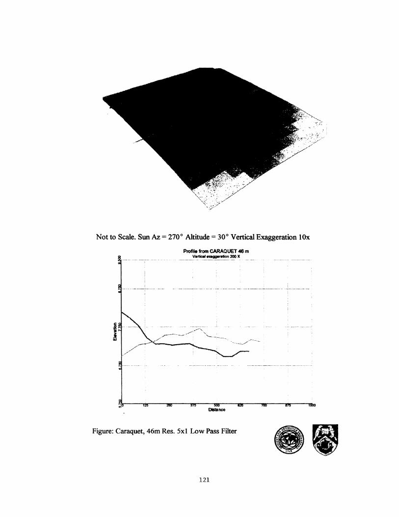
Not to Scale. Sun Az = 270° Altitude= 30° Vertical Exaggeration lOx
Profile from CARAQUET _. m Vertical........,n 200 X
Figure: Caraquet, 46m Res. 5xl Low Pass Filter
• .
. .
121

·~·
Not to Scale. SunAz = 270° Altitude= 30° Vertical Exaggeration lOx Profile from CARAQUET 46 m v~~.~~on 200-~-
.. -·- ---------- --- --··------/~- -··:
I\ I \ .
/ '• I \ \j \ I
·-··- --\ ' .... /-------'------\ I
Distance
Figure: Caraquet, 46m Res., Fourier
122
• .
-

Not to Scale. Sun Az = 270° Altitude= 30° Vertical Exaggeration lOx
I
Profile tam CARAQUET 5m Verbi.,....,.._200X
J d~o-------ft,Mr-----~~--------~szr' ------~~r------,118~·~--~,RMdbo
Distance
Figure: Caraquet, Random TIN Densification, 10-2
123
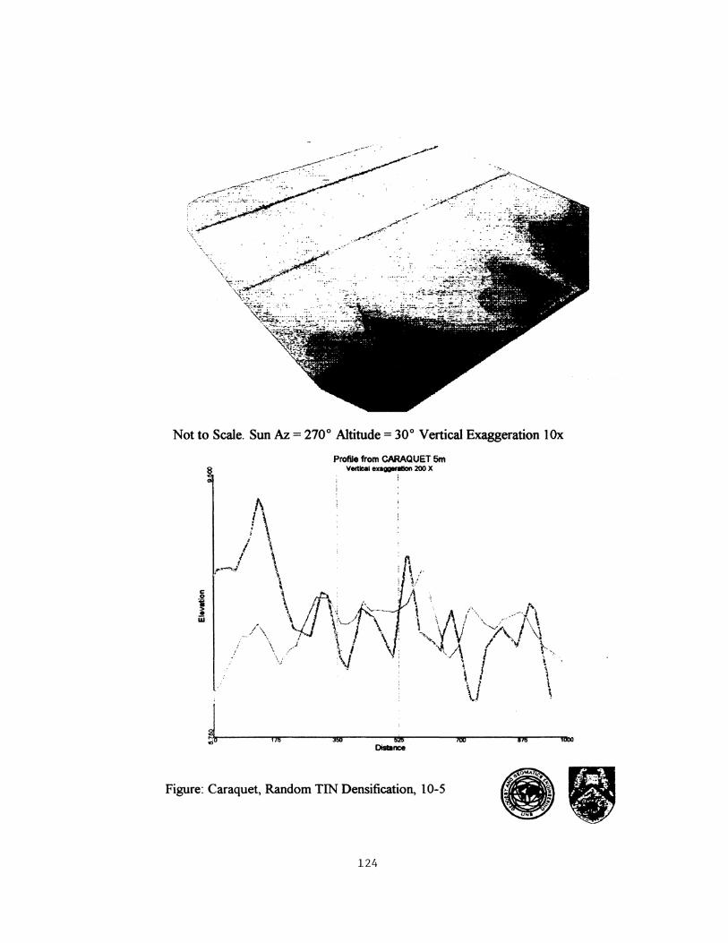
\ ..... ·. '-
--......
Not to Scale. Sun Az = 270° Altitude= 30° Vertical Exaggeration lOx
8
t/6
Profile from CARAQUE.T 5rn VetUclllexaQIIRIICin 200 X
Figure: Caraquet, Random TIN Densification, 10-5
124
IW 11! itiUO
•

Not to Scale. Sun Az = 270° Altitude= 30° Vertical Exaggeration lOx
-,.......,------~ ----------- -~--~~-~ ~~~ ~
Figure: Caraquet, Trend Surface, Order= 3 Vertical Exaggeration = 200x
125
;

.. ··-···..,., . _J
._, .
. :--~··
~······~ .... -. . -< .... -·
Not to Scale. Sun Az = 270 o Altitude = 30 o Vertical Exaggeration 1 Ox
Profile from Whitestar Vertical exaggeration 200 X --- ---- .. --~----·- ··--:----·-·------:-------~-- ------------ -·-- --~
Distance
Figure: Caraquet, 46m Res., Filtered by Whitestar Inc.
126

Not to Scale. Sun Az = 270° Altitude= 30° Vertical Exaggeration l.Sx
Figure: Aroostook, TIN
Profile tram AROOSTOOK !5m V.UC.Iexegger8tlon 8.0 X
127
• ' .
.
.

Not to Scale. Sun Az = 270° Altitude= 30° Vertical Exaggeration l.Sx
Distance
Figure: Aroostook, TIN
• .
,. .
128
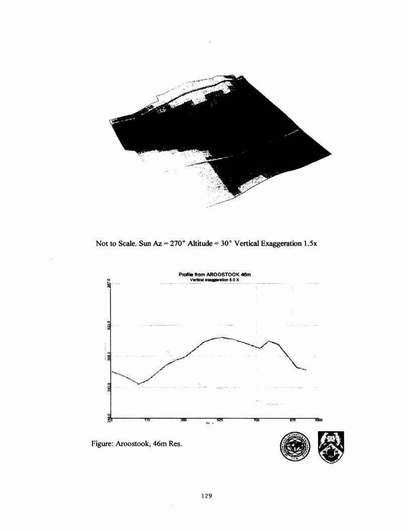
Not to Scale. Sun Az = 270° Altitude= 30° Vertical Exaggeration l.Sx
Profile from AROOSTOOK 46m 0 !ft·--- veracale.....,.aon e.o x
... ········-···-·- . ·-----·-······-·· ....... ··-·--·--·--
··~ ' ...
Figure: Aroostook, 46m Res.
• .
. .
129

Not to Scale. Sun Az = 270° Altitude= 30° Vertical Exaggeration l.Sx
Profile from AROOSTOOK 46m V81tic81-ggeretion 6.0 X
.... --------- ·-------------------------- ... --- ---···-------·· .. ---------------- ------ ··----------------- ---- ----'
Figure: Aroostook, Sxl Low Pass Filter
• .
.
130

Not to Scale. Sun Az = 270° Altitude= 30° Vertical Exaggeration l.Sx
Profile from AROOSTOOK .c&n Vertic:aleaggeration 6.0 X
.-----------.
\ , ..................... ::.;_ ................. .
\..
Figure: Aroostook, Fourier Transform
131 • .. . .

Not to Scale. Sun Az = 270° Altitude= 30° Vertical Exaggeration l.Sx
Profile from AROOSTOOK 5m
·~··---·-········· -----~v-J
Figure: Aroostook, Random TIN Densification, I 0-2
• ' -
132

Not to Scale. Sun Az = 270° Altitude= 30° Vertical Exaggeration 1.5x
Profile from AROOSTOOK 5m Vertica!.!_xaggerdon__ _ e.ox _______ " ____ _
Figure: Aroostook, Random TIN Densification, 10-5
133

Not to Scale, Sun Az = 270° Altitude= 30° Vertical Exag = l.Sx
... --~------ ... --·--·-·--·----·-··-·--··-······ ····- -.----
__./! ' \ ' \
.1
Figure: Hayesville, TIN
134

Not to Scale. Sun Az = 270° Altitude= 30° VE = l.Sx
. ······-··--:--. ····-·-·-·- --·-· -r-·-- ·--··-··-
Figure: Hayesville, 46m Res.
1
\
' ' ' ... ····t·-----------. L .. ---·····
\ \
\ . ~--·---.,
135

-e.~ -~-,
Not to Scale. Sun Az = 270° Altitude= 30° VE = l.Sx
Figure: Hayesville, FFf.
Vertical Exaggeration= 7x
136
• -
.·

Not to Scale. Sun Az = 270° Altitude= 30° VE = l.Sx
-----·--·-·· ---·y_.::::;·--~:::; -----~----- ---··----- ···--···- --·- ·----~---·-----------······ ·-···--· --·--···-_,.,... ; \,\
,-/'/ \\
/ i
r I
"" cD -------·--·· --··-- _____ J... _______ ....... .-:. _______ _
\_Vertical Exaggeration F 7x
' . ·-.
Figure: Hayesville, Random TIN Densification 10-2.
• .
-
.
137

... ~- .. ·· .
. . -~:~· : :
\.;· .. ·~· .... ·."'.. ~ -·'· ·.
! .
Not to Scale. Sun Az = 270° Altitude= 30° VE = l.Sx
r:==/7~~:~-, ----. -:--r
\i
350.0 525.0 700.0 '<
875.0 986.1
Figure: Hayesville, Random TIN Densification 10-5.
Vertical Exaggeration = 7x
138

Image A: Aroostook Study Site - TIN contaminated with Ridging.
Image B: Aroostook Study Site- Randomly Densified TIN.
Figure: Random TIN Densification, Testing: Comparison in Region of High Relief.
139

APPENDIXE
Analysis: Phase II - DTM Plots
140

t-' +:'t-'
_.,. ... ~-·
, _.i~;,.:. ... ol'-·""
~-::.:.·· ..
_.~~··
:.· ... .. -~ .. ... ,.~ --· ,,
·'~ .. .~
/
Caraquet: CTM Fourier Filtering
. ./ "iJ,..- .... __ 4 ••• /~
/
/ _../
, ...
_,·
.•
~:.-:··:~ _.rv::·~~~~ 1;;,·· ..
···:<'-·~·.:.;l:;:~~~t::~_('>'; ·~ >.:·..;.~··· ......
. . .-~"·~: .·- .. __ . ~
.... '" ..... -~ .... ;;;'? •. ,. • ...... ~:
~/;:,:·:.·:~;;•"":.'~ .-·-........ . ...
:.~ ...
I . . ·

• -.
142
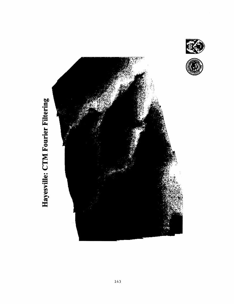
• .
.
.
143

APPENDIXF
Histograms
144
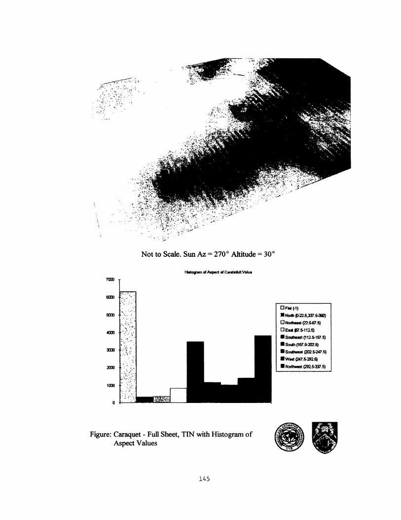
Not to Scale. Sun Az = 270° Ahitude = 30°
Figure: Caraquet - Full Sheet, TIN with Histogram of Aspect Values
145
0 Fill f-1)
• NOIIh P-22.5.337.53110) EJ No!lhelllt (22.5-67.5)
0Eattli7.S.1125)
• Sodhealt (112.5-151.5)
.ScMh{151.S.:l02.5)
·~· (202.5-241.5) •wut c,w.S-2!12.5)
• N""'-1 (292.5-337.5)

..... ~--: ~·· ·~·. '
.~ .......
Not to Scale. Sun Az = 270° Altitude= 30°
Hlst.-n or Aapect or CIIIIII0-2:VIIut
Figure: Caraquet - Full Sheet, TIN Random Densification 10-2, with Histogram of Aspect
Values.
146
DFIIt ~f)
• NOIIh ~22.5,!37.S.3Ei0)
El Nortllttst (22.5-87.5)
0 Etst tu.S-112.5)
8 Southatst (112.5-157.5)
• South (157.S.:m.5)
8 Sout'-11 (202.5-2~7.5)
•·wast (2~7.5-292.5)
8 NorthMst (292.$337.5)
• .

Not to Scale. Sun Az = 270° Altitude= 30°
Figure: Hayesville- Full Sheet, TIN, with Histogram of Aspect Values.
147
EIFitt (-1)
• Nadft P.22.5,337.5-311l)
0 NolthRit (22.567.5)
0 Ent fi7.5-H2.5)
• 5cKllltUt (112.5-157 .5)
• &uh (157.5-312.5)
• SdM.It (m.S-:W.S) .w ... (247.5-292.5)
.No!t~Mast (292.5-337 .5)

Not to Scale. Sun Az = 270° Altitude= 30°
Figure: Hayesville - Full Sheet, TIN Random Densification 10-2, with Histogram of Aspect Values.
148
Ia Rat (-1)
• Nollfl f}-22.5;337.5-300)
Gl Nollhlallt (22.5-67.5)
DE811 f37.5-112.5)
·~heallt (112$-157.5)
• S!Mh (157 .5-2112.5)
• S!Mhwelt Cll2.5-247.5)
•waat (247.5-292.5)
• N..o-at (292.5-337.5)
11 .... , " ,. . .
H • .
.

APPENDIXG
Scatter Plots
149

Caraquet 5x1 LPF Comparison
1 0 ~-·-. ......... ·-·- .. --· ·-·· ·- --······- ········--···. -··- ---·.-----·-··----··----·-···-----·---------·-··-----·-··-·-· ····-···--·-···---·--- ----· ... ·--·--······ --···········-··-····----·····-· -.-··-
3+-------------~------------~--------------~-------------r-------------,------------~ 3 4 5 6 7 8 9
5x1 LPF Elevations (Metres)

c: 0 .,
"1: CIS Q. E 0 0 ... CD "1: :II 0 u.. -.; :II CT f CIS 0
0 ......
•
•
• •
• • •• CIO
• • • ····:: • •
.. I ••• • .,, ..... • • • • ,.:. • •• •• • • • 4 • • • • ••• • • • • "i' • ~ • .. • • • ~ ... ., •• c::
• co 0 ";::;
• ~ • ~ iii lL 1-• lL
1.0
(sa.qaw) suO!:JBAal3 paJa:JnJun
151

Caraquet TIN Random Denification Comparison - 2 Points per Original
10 ~----------------------------------------·
9 I •
• • • • 8 .• ;,··· •
i t-' il .... ~ iJ1 !. N
Ill 7 c 0 ••• :;::; , ... Cll ... ~. > • • Gl ijj • i 6 • .. ! •• • ;;::
4llt c ~
5 • • • • •
4 I • • • I
3 3 4 5 6 7 8 9 10
TIN_RD Elevations (Metres)

I !
I ! I ! I I !
•
I I I
I 7i c: ·o, "i: 0 ... G) c. l! c: 15 0.. 10
c: 0 1i () li: ·; c: ~ E 0 '0 c: aJ a:: z i=
I ••
•
• ~.
:-.. .. t:. ' . ~ ~ ... ' \ • ' •
IX)
153
• •
• • • ••
• ••
•
0 .....
IX)
... r-- G) ... • ~
c 0 ;::;
• IV > G)
iii Q a:
<0 z' i=

m
00
• • Ji .. • • I ... ., ....
• -~· • • • ... , • • • • • c
I 0 • • 'i: -• " -~ :::E a. -E ... • 0 c 0 0
~ CD • • E u co ~
'· iii
:I • • 8 U) • -! "D • c :::1
! • U) "g 1- c
'&) • ! :I • t-C" l! • " • • 0
• •
• •
0) lO
S8J~8W) SU0!~8A813 paJ~I!JUO
154
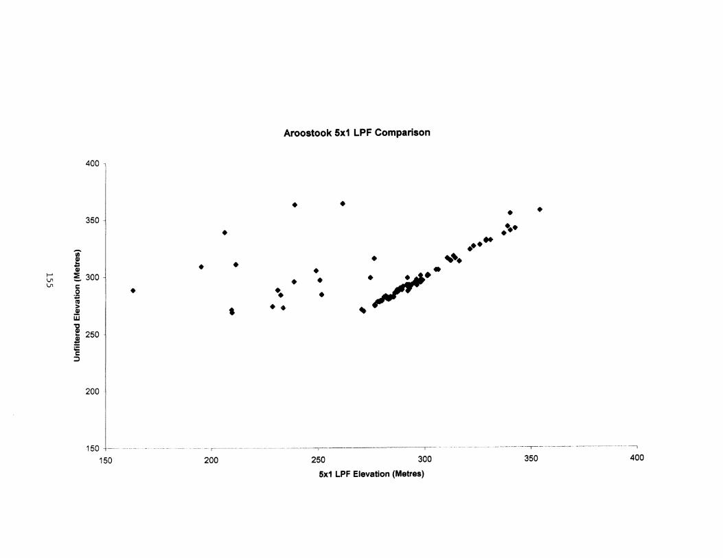
I-' 1..11 1..11
400
350
i .1:1 Gl !. 300 c 0
:1:1 111
~ w
~ 250 s iE ::;)
200
150 --r----
150
•
Aroostook 5x1 LPF Comparison
• • • • • .... . ... •
• • • •
..... • • .·/·· •• •
• • •
----. - ---- -- r--------------------------· ---------,-
200 250 300 350 400
5x1 LPF Elevation (Metres)

Aroostook Fourier Comparison
390 ·-----------------·· .. --
370 I
• • • •
- 350 I
Ul ~ Qj
t-' !. V1 0'\ c 330
:8
• •
• • •
• • • • • I'll
> .! w 1! 310
• ..
• •• • • • • • •
• • ~ ;;:: c
:::::> 290 '
• • • •
• \\Sf·· • • •t
• •
270 ~
•• .... • :
' ... , • • • I
•
• • ••
• • • • •
250+-------~,-------~---------r--------~--------~--------r--------,--------~--------~
250 260 270 280 290 300 310 320 330 340
FTF Elevation (Metres)

1-' V1 "'--
390
370
350 i .. li :::E ~ 330 0
:;:1 Ill
1 w i 310 .. :@ ~ c :::1
290
270 ·'
Aroostook TIN Random Densification 2 Points per Original
.,// ~ .. . ,# •• • -
• ••• ••
-·----
•• • •
250+-----------r-----------r-----------r-----------r-----------r-----------r---------~
250 270 290 310 330 350 370 390
TIN_RD Elevation (Metres)

1--' V1 CXl
390
370
350 Ui' Gl ... ... Gl :E ._.. c 330 .2 ... l'a > Gl w "0 310 ! ! iE c ::)
290
270 ••• •••
Aroostook TIN Random Densification 5 Points per Original
~·· /.,.,.. ~, ,
• • ••
• • • • ••
·-·-----------·]
• •• •
250+---------,---------~--------,---------.---------,---------~--------~
250 270 290 310 330 350 370 390
TIN_RD Elevation (Metres)

APPENDIX&
Analysis: Phase II- Contour Plots
159

Image A: Contours generated from a TIN that is "Contaminated" with Ridging.
;: ~ .
~7: .·' ....... I {~'\. \·'.1~'\\\..'\/ ~:"' /'\ J'.·-...·..j~ ~ ·- ...... · i .r"':: ~~-· ·>,! . -..:;··;li;i ·,· ;,.:_:\\'• ·-·· .... ~· ,./ ... , '·; •· r,: •. -_ .... -.... ta-. ~~~~ ..... f<' \t , _.:• "'\ ""// • ..... .-J'~"rj
~::~:-~;-~~;.~ G,\)1'1._~<,_-_·T·,~'?~F ----~,. ~:·-~~ /·-:;;:;~--~/
Image B: Contours generated from a randomly densified TIN.
Image C: Contours generated from CTM Fourier Filtering.
Figure: Caraquet. 0.5m Contour Comparison
160

Image A: Contours generated ftom a TIN that is "Contaminated" with Ridging.
Image B: Contours generated ftom a randomly densified TIN .
. ' . ·. : ~ .'
. ; ·<.·.-·-
.---·. · .. -- ..
Image C: Contours generated ftom CTM Fourier Filtering.
Figure: Aroostook. 3.0m Contour Comparison
161

Image A: Contours generated from a TIN that is ''Contaminated" with Ridging.
Image B: Contours generated from a randomly densified TIN.
Image C: Contours generated from CTM Fourier Filtering.
Figure: Hayesville. 3.0m Contour Comparison
162

APPENDIX I
Analysis: Phase II - Hydrological
163

1-'
"' ~
/ .!"
/. · ... .. ,(
''
: ·~:;-/ :.,•'
'1 ' .... ....._, !. ; ·~---.·}
···~ -rr.~ . . ' ......
\·
.r'i· :·-:.-· .. ;"$.! ~-:·: ...... ··· ', .. •: .• / i ' • ''''f}. '·· ' /t . ·; . .S~ _~,· : .. · :·~ >-~ .. .:: \__;:
,'':ii:' .. ,;-..... ~·\
/~· ..
/:,
. \ ·' ·.' ~~\- p~>-··· ...... ··- -.... ·,_: ·,,_..._~·5·\~ _ ... ~-
'· '· · .... ·· .. ~:
t, -z..~-~·'"' ---~-... --'·--~-~ ....
\. ~ ·-. ... ·.~·-.
., ... ··~-.. ~; -~·:- .. ............... . .. ·''
;-(,t< :' :::::;"'\;;~~1~1 . _..,·-;:····-~~ '7-~;_.,t;i~- ); .. {.:
... // -~.~: :·· .. c.:~ .<·~ft;~~--~j;~~; ./.. . • ! ., :'·y:-r ·H'h:~l: : " ; · ..J J , ., ·, J. ,. •· ·. I •' · , .. 1 •o·• · ·;:. / ·-:,:.:f:·):\t,v-1,;~}~~-~~~:~1~t:i·; -~. li. r;:~::: __ ...,.~~:. ~r;~.,; ... · .. .
.. • .-"'v . ' . ":, -~i'.'( • \4 .j;'' l' ,,tl·;,, [~~ • .'. •f' .J • '• I ~ I : ""·~··•>' . I ' . ., . , . .-· ·' . •< ' . '... '• . ,, . . •• . . ·~ l . • ... ·" ..... , > . "::- . ; . .i' ;;, .:; ···: . .. ! '' ,. \ ': ,:. :•·q:.li:f ;..J!i ~·f":f ··.' .. -;r:. ; ; < - . "1 '··' ' ·. . ( :: ~:'(. . ' ;. . .. :; i ~,,, :_ . -·- . ; . ' ,• . . . '. "1-·'ll'' . - . . , ··~· ·~· _:L··~. ::it'~" / ___ 'J.i.L ,
Figure: Hydrological Analysis Caraquet: Unfiltered DTM
300 0 300 ~ Meters e i
Legend
I Eaater1y Flowing Stream I ~FlOWing Stream I Westerty Flowing Stream ! Northerly Flowing Stream
rAJ •

...... 0'\ V1
' • ."1.'
·<
:;~~;: · · ... tr;· ;.;. .:.-.. :-..... ...,.., '- t..::-'·' ~~:····."~:~- ·.iJ! ·:_]&.:'-' . :~£ .. -.:; ··; :·:·-·
.. ~-··-=--· .
. , '
:::.;£.
~ ... ~; .
___ .... ,) =
~1: ...
700 0 700 1400 Meters - --
Figure: Hydrological Analysis Caraquet: TIN Random Densification 10-2
Legend
I Easterly Flowing Stream I Southerly Flowing Stream I Westerly Flowing Stream ~ Northerly Flowing Stream
I . '

f-' 0\ 0\
.. ·~~ ("
700
Figure: Hydrological Analysis Caraquet: CTM Fourier Filtering
0 700 1400 Meters
Legend
I Easterly Flowing stream 1 Southerly Flowing Stream 1 Westerly Flowing Stream I Northerly Flowing Stream
I .
.
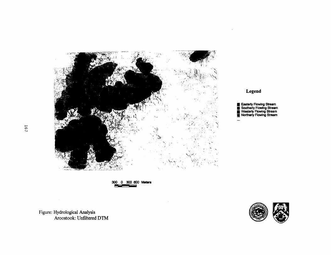
...... 0'\ -...J
Figure: Hydrological Analysis Aroostook: Unfiltered DTM
) ~·
'· ....
300 o 300 eoo MeWs
!I"Si4 -
:./: ':-.·
i ·~. ·• .. .. ';:~:.:;~;;~&r~·•••·"~
.... , . .r:. '::·
•'1.-r.
•.:.; j'
·...:.··- .·i'
····-
'-.\1 ''• ·~:
. ~.·: ? .. ;\,~;
.. ......
. ·~ .· . .::)·i;: ·'. ··'' ·. :> ·.:· .
•.
'.\ .•• <;-·.:·
'
·' . ~·· . . ... · .: 't~;:·. . ·'·~ '·. •' ..
·., .... ,. : ~' ..
.,\,. , .. '.-" ... ... ,. I • , .... ~ .. :.··:
:' ... ~ ~ ..
.... ._..
·,·+·: , . .,.
··\ . .....
"
~ ,•
' ··. \
Legend
• Eastet1y Flowing Stream • Southerly Flowing Stream • Westerly Flowing Stream • Northerly Flowing Stream
I . .

t-' (j\
00
j .. ·'
Figure: Hydrological Analysis
'\'\~: ···.".il-
''\·
. '\;· .... : .. :}:.;·.
··.• •'!.
·.·1 . . ' -~
" . · ... ~:::: ..
-:::.
. ~-···t
'· . . ·~:·., ..... :''; >': . ~ . '-" . . ,I ' ·'}'·:·.-.\., ~;· '· ~;·J
_./i;;>:S .. '-~i · ;.':·\ ·'-•' • 1
: · .. • :. . .. _.,::._ \! ) ,,·~.I '\,_>
. -.•. \ ·,-:_~}~~('
'· ,,. ?;
,. ' '
.. ·:'· ... · .. :~ .. :·· .·, .. ·:· -:(· '':\:f:.· ;,
.. . :-:.~;.z \
i I
Dl o 300 eoo Meters e
--~ ·-.: ·.:·:~:::·'-1 ~' -~tt-. ... :···· .. , .. ''·
Aroostook: TIN Random Densification 10-2
Legend
I Easterly Flowing S1ream I Southerly Flowing Stran I Westerly Flowing Stream ! Northerly Flowing Stream
I '
.

1-' 0'\
"'
Figure: Hydrological Analysis
700 I!!!
Aroostook: CTM Fourier Filtering
0
' ~ < ;. -. . ':. ·<r':':.::, <~::
'~·) ·"'·~:. ·i:::,.:_\1rj~ ·"'" ''~ ... . "'1.\"'.,.~r '"' ;(,;. < ·r~r' ,,;.
·:;~. ..· .. · ··I · .... ·· .. ·
·)._, r·-·.··
·~·.
-- -.~'··: ·. \ .. . ~ ....
' . _, "\~ .. ~: ~~'~:\~~~-,.
\ ,,,~;{(~ '>~: ,. :I " .·;~;·.
_It_
·.·. ' .
.... , .. ;_,(~ "';~, .-- , ..... ~ ·-
700 1400 Meters
Legend
I Easterly Flowing Stream • Southerly Flowing Stream • Westerly Flowing Stream ,! Northerly Flowing Stream

'"'"" -...J 0
'' i
Figure: Hydrological Analysis Hayesville: Unfiltered DTM
:_, .. ....
300 o 300 eoo Meters I'"'"- I
;:....-:· ...... . ~ .. )~:~ -~~~~ ·•. '·
. :.... . ~;. ·_; . ~ ..- .t: .. ..... '.:
Legend
• Easterly Flowing Stream a Southerly Flowing Stream I Westerly Flowing Stream !J Northerly Flowing Stream
I ' .

1-' "'-I-'
Figure: Hydrological Analysis
D) 0 ~ 600 Meters t"1
Hayesville: TIN Random Densification 10 -2
Legend
I Easterly Flowing Stream I Southerly Flowing St'-'1 1 Westerly Flowing Stream I Northerly Flowing Stream
I .
.

~ -...J N
700 0 700 1400 Meters
Figure: Hydrological Analysis Hayesville: CTM Fourier Filtering
Legend
- Easterly Flowing Stream - Southerly Flowing Stream - Westerly Flowing Stream - Northerly Flowing Stream
I . . .

Vita
Candidate's Full Name:
Place and Date of Birth:
Permanent Address:
School Attended:
Universities Attended:
Degree Obtained:
Colleges Attended:
Diplomas Obtained:
Kevin Huntly Pegler
Weston, Ontario Canada 19 Apri11961
175 Topcliffe Crescent Fredericton, New Brunswick E3B4P8
King City Secondary School King City, Ontario
Ryerson Polytechnic University Toronto, Ontario
Bachelor of Technology Survey Engineering June 1994
Algonquin College Ottawa, Ontario
College of Geographic Sciences (COGS) Lawrencetown, Nova Scotia
Dipl. GIS (Honours) May 1995
Graduate Dipl. Remote Sensing May 1996
Publications: Pegler, K., D. Coleman, and R. Castonguay (1999). "TIN Random Densification: A Process to Minimize the Ridging Phenomenon in DTMs." Proceedings of the 1999 URISA Annual Conference, Chicago, Illinois. (August 20-26) pp. 223-230.