an experimental approach to teaching the concept of
TRANSCRIPT

East Tennessee State UniversityDigital Commons @ East
Tennessee State University
Electronic Theses and Dissertations Student Works
5-2002
An Experimental Approach to Teaching theConcept of Functional Diversity.Cory McKelvey StanleyEast Tennessee State University
Follow this and additional works at: https://dc.etsu.edu/etd
Part of the Biology Commons
This Thesis - Open Access is brought to you for free and open access by the Student Works at Digital Commons @ East Tennessee State University. Ithas been accepted for inclusion in Electronic Theses and Dissertations by an authorized administrator of Digital Commons @ East Tennessee StateUniversity. For more information, please contact [email protected].
Recommended CitationStanley, Cory McKelvey, "An Experimental Approach to Teaching the Concept of Functional Diversity." (2002). Electronic Theses andDissertations. Paper 637. https://dc.etsu.edu/etd/637

An Experimental Approach to Teaching
the Concept of Functional Diversity
A thesis
presented to
the faculty of the Department of Biological Sciences
East Tennessee State University
____________________
In partial fulfillment
of the requirements for the degree
Masters in Science
by
Cory McKelvey Stanley
May 2002
Foster Levy, CoChair
Cecilia McIntosh, CoChair
Dan Johnson
Keywords: Teaching, Biological Diversity, Functional Diversity, Conservation, Science.

2
ABSTRACT
An Experimental Approach To Teaching The Concept Of Functional Diversity
by
Cory McKelvey Stanley
This study tested an experimental approach to use in teaching the concept of functional diversity. The project culminated in a laboratory exercise for use in high schools. Experimental design consisted of representatives of 3 functional groups of plants, (legumes, grasses, and forbs), planted singly, and in 2, or 3 species combinations. Legumes were represented by Trifolium repens and Medicago lupulina, grasses were represented by Cynodon dactylon and Festuca rubra, and forbs were represented by Helianthus annus and Raphanus sativa. Plants were grown inside a controlled growth chamber. During the growth phase, measurements were taken to highlight temporal differences in development. After 2 months, wet and dry weights of aboveground and belowground portions were measured as indicators of productivity. Research showed unique developmental patterns of functional groups. Secondly, functional combination, not functional group number, produced a significant difference in biomass. Laboratory use involves group discussion, active-learning, and higher understanding of conservation.

3
CONTENTS
Page
ABSTRACT... ........................................................................................................................ 2
LIST OF TABLES................................................................................................................. 5
LIST OF FIGURES .............................................................................................................. 6
Chapter
1. INTRODUCTION .......................................................................................................... 7
The �Big Question�..................................................................................................... 7
Restoration Techniques and Functional Diversity...................................................... 8
Recent Studies............................................................................................................. 8
Global Effects ............................................................................................................. 10
Goals�. ...................................................................................................................... 11
2. MATERIALS AND METHODS .................................................................................. 15
Experimental Approach ............................................................................................. 15
Initial Trial (Field) .............................................................................................. 15
Second Trial (Growth Chamber) ........................................................................ 19
Final Trial (Growth Chamber) ............................................................................ 19
Biomass Assays ......................................................................................................... 22
3. RESULTS ...................................................................................................................... 24
Temporal Development ............................................................................................. 24
Plant Biomass............................................................................................................. 31
Functional Group Variance........................................................................................ 36

4
Chapter Page
4. DISCUSSION ................................................................................................................... 43
Classroom Adventures .............................................................................................. 43
Methods...................................................................................................................... 44
Growth Area............................................................................................................... 45
Data Collection .......................................................................................................... 46
Data Presentation ....................................................................................................... 47
Functional Group Number ......................................................................................... 48
Functional Group Combination ................................................................................. 49
Less Variance, More Stability.................................................................................... 50
Concluding Remarks.................................................................................................. 50
BIBLIOGRAPHY.................................................................................................................. 53
APPENDICES ....................................................................................................................... 54
Appendix A: Lesson Plans for an Inexpensive Experiment on Functional Diversity. 55
Appendix B: Data Table for Bi-weekly Analyses .................................................... 61
VITA................. ...................................................................................................................... 62

5
LIST OF TABLES
Table Page
1. Trial 1 Field Design .................................................................................................... 17
2. Time, Temperature, and Light Settings for the Growth Chamber����..��� 18
3. Trial 3 Design ............................................................................................................. 20
4. Spacing for Pot Growth Conditions ............................................................................ 21
5. Results of One-way ANOVA to Test the Effect of Number of Functional Groups on
Aboveground Dry-weight Biomass ........................................................................ 32
6. Results of one-way ANOVA to Test the Effect of Number of Functional Groups on
Aboveground Dry-weight Biomass ......................................................................... 32
7. Results of One-way ANOVA to Test the Effect of Number of Functional Groups on
Belowground Dry-weight Biomass.......................................................................... 33
8. Results of One-way ANOVA to Test the Effect of Type of Functional Groups on
Belowground Dry-weight Biomass.......................................................................... 33
9. Growth Pot Combinations.......................................................................................... 34
10. Results of One-way ANOVA to Test the Effect of Number of Functional Groups on Total
Dry-weight Biomass ................................................................................................ 35
11a. Results of One-way ANOVA to Test the Effects of Type of Functional Groups on Total
Dry-weight Biomass ................................................................................................ 37
11b. A Posteriori (Tukey�s) Test to Show the Location of Differences Associated with the
One-way ANOVA... ................................................................................................ 37
12. Results of the Test of Homogeneity of Variance Between 1, 2, and 3 Functional
Groups����������������.��.����������� 41

6
LIST OF FIGURES
Figure Page
1. Alfalfa: Number of Leaves in Pure and Mixed Culture............................................... 25
2. Clover: Number of Leaves in Pure and Mixed Culture .............................................. 26
3. Bermuda: Number of Leaves in Pure and Mixed Culture .......................................... 27
4. Fescue: Number of Leaves in Pure and Mixed Culture .............................................. 28
5. Sunflower: Number of Leaves in Pure and Mixed Culture ........................................ 29
6. Radish: Number of Leaves in Pure and Mixed Culture .............................................. 30
7. Total Aboveground Dry-weight Biomass per Number of
Functional Groups..................................................................................................... 38
8. Total Belowground Dry-weight Biomass per Number of Functional Groups.............. 39
9. Total Dry-weight Biomass per Number of Functional Groups .................................... 40
10. Mean Biomass per Number Functional Groups (+/- SEM).......................................... 42
7
CHAPTER 1
INTRODUCTION
The �Big� Question
Recent controversy in the field of conservation biology stems from the question: Is the
number of species (biological diversity) more important to maintaining ecosystem stability and
productivity than the number of representatives or combinations of different functional groups
(functional diversity/functional composition)? Biological diversity can be defined as �the variety
of living organisms considered at all levels of organization, including the genetic, species, and
higher taxonomic levels, and the variety of habitats and ecosystems, as well as the processes
occurring therein� (Meffe 1997).
Functional diversity can be defined as the variety and/or combination of phenotypic
characters contributing to an organism�s or a community�s survival and productivity. Functional
group delineation consists of placing organisms with similar functions into the same groups. The
questions and controversies behind the biological and functional diversity argument highlight
differences in the environmental and emotional values of biodiversity. The goal of maintaining
biological diversity is inherently attractive scientifically because extinction of a species results in
the loss of unique genotypes. Similarly, biological diversity appeals to emotional values held by
many people, because as human beings we tend to strive to protect other organisms from harm or
extinction, rather than to destroy things around us (Wilson 1984).
8
Restoration Techniques and Functional Diversity
The ultimate goals of a pragmatic conservation program are to protect and restore ecosystems
while maintaining productivity and sustainability of local and global communities. In the search
for innovative restoration techniques, several groups of scientists have studied the effects of
functional diversity on ecosystem processes. Categories for defining functional diversity
include: morpho-physiological similarity, functional roles, functional combinations, and
functional groupings. The morpho-physiological basis of different organisms characterizes their
effects on surrounding organisms based on physical, biochemical, or genetic factors. The effects
on the environment may be positive, negative, or nil. The functional role of any organism is its
overall effect on an individual level, a community level, or even on a global scale. Functional
combinations are the mixtures of different functional roles in a community. These varied
combinations are at the heart of both this study and the future of conservation biology. Tilman et
al. (1997) stated that certain aspects of plant growth and productivity including, percent nitrogen,
plant total nitrogen, and light penetration were affected by functional diversity and functional
composition. With this in mind, major environmental changes can occur through the alteration
of functional diversity and functional composition.
Recent Studies
Recent research efforts in conservation biology have been directed toward measuring and
comparing biological diversity because selected species may gain additional security from local
extinction by having more biomass through increased biological diversity (Naeem and Li 1997).
A more recent study suggests that functional diversity is more important than species diversity in

9
ecosystem processes (Tilman et al. 1997). Hector (1999) also found that there was a reduction in
the amount of aboveground biomass as the number of functional groups decreased.
Most studies to assess the role of functional diversity were carried out in large field plots,
manipulating the numbers of species, functional groups, and functional group combinations.
Past studies showed that the number of functional groups as well as the unique functional group
combinations produced a greater change in aboveground biomass production than did the
number of species in the field plot (Tilman et al. 1997). Larger studies can last a number of
years, including a 7-year experiment that contained plots of 16 species, which gained 2.7 times
more biomass than a monoculture (Tilman et al. 2001).
Almost all-recent studies have used the similar methods of combining different functional
groups in field plots to test effects on resultant biomass. Biomass production was the main, and
sometimes only, measure of productivity recorded in these field studies.
Three functional groups (forbs, legumes, and grasses) represent the only functional groups
used and identified for research purposes in past studies, and they are included in this study
because of their near universal recognition. Legumes represent species harboring nitrogen-fixing
bacteria, which bring fixed nitrogen to the plant roots. As these plants decay, fixed nitrogen is
added to the soil. Grasses often contain smaller leaf blades than forbs, which allow more
sunlight penetration through the canopy, as well as massive root structures that create crowded
root growing mediums. Forbs, like many other functional groups, are somewhat lacking in
concrete characteristics, other than the fact that they are very different from the other 2
functional groups. Two species representing the legume group were alfalfa (Medicago lupulina)
and red clover (Trifolium repens). The 2 species from the grass group were bermuda (Cynodon
dactylon) and red fescue (Festuca rubra). The forb group representatives were radish (Raphanus

10
sativa) and sunflower (Helianthus annuus). Many other species, including forbs, require further
research. Some of these same species and functional groups have been used in other studies.
Examples include C4 (warm season) and C3 (cool season) grasses that present different growth
processes and possibly different functions. Identification of other functional groups are at the
forefront of research, and their identification will be a major step for the proper combining of
functional groups to create more stable and productive ecosystems. Possible groups may arise
concerning developmental time, root growth patterns, decay patterns, spore production, or plant
color. Students should have the opportunity to develop their own ideas.
Global Effects
Determining the value of functional diversity is an important focus of conservation biology
research, mainly because of declining ecosystem stability and the increasing human population.
Human expansion causes not only a loss of biodiversity (Naeem et al. 1994), but in recent studies
it has even produced predictable functional shifts as new traits are replacing old ones (Loreau et
al. 2001). This loss of diversity is a loss of life, as well as the loss of rare and perhaps
functionally important species. Many times there have been alien species introduced into an
ecosystem, and the invader would completely take over the system and drastically decrease both
species diversity and functional diversity. Functional groups are not completely defined. For
example, unnamed functions of rare species may be important to ecosystem function as
evidenced by the observation that removing rare species from certain communities has been
shown to cause an invasion of exotics (Lyons and Swarts 2001).
Conservation biology is also in dire need of more research directed toward understanding
varying types of functional roles that may define an ecosystem, and how the roles may or may

11
not be combined. China�s serious, yet undefined problem with rice production was partially
answered by simply growing two different strains of rice together, one standard strain that does
not succumb to rice blast fungus, and another more economically valuable strain that does (Yoon
2000). The 2 strains filled functional roles that, in combination with one another, assisted in
boosting total growth and productivity. Functional roles of these 2 rice plants were straight-
forward. The more economically valuable sticky rice plant was tall and enjoyed sunny, warm,
and dry conditions. The standard disease-resistant rice plants were shorter, allowing the sticky
rice plants to have optimal conditions and become less prone to disease because the spores were
not traveling between rows or fields. This is a simple functional combination, involving plant
height characteristics, a struggle for resources, and blocking of airborne spores while in a
heterogeneous mixture instead of a homogeneous mixture. In theory, optimal combinations of
other functional roles could help agricultural systems to increase stability and productivity of
food producing species (Yoon 2000).
Increased productivity could assist in filling needs for resources to support the increasing
human population, which is causing a degradation of our biosphere, and an extinction of
organisms and the habitats in which they live (National Research Council 1992). Economics
may be linked to functional diversity research, because as the rice project has shown, functional
combinations can increase biomass production in crop species. Therefore, farmers and
corporations can be expected to fund related research projects.
Goals
The goal of this study was to design and analyze an experiment that could be adapted for use
in a classroom setting in order to educate secondary education students about the concept of

12
functional diversity. Activities related to preparation of experiments and gathering different types
of data had the beginner student in mind. Three observable plant growth measurements (number
of leaves, length of largest leaf blade, and shoot height) that were based on easily recognizable
characteristics were used throughout the entire growth phase. Having students measure the
plants during the growth phase would allow the students to stay actively involved in a weekly
task while observing and comparing growth characteristics.
Research is commonly seen as an overwhelming task, but when the task is broken into many
smaller parts and a class is divided into groups, a more positive feeling toward research may be
achieved. As the experiment is broken down into smaller components (planting, growing, and
final data collection) the components can be used in a cooperative classroom where students
assist each other in reaching a common goal (Henton 1996). In addition to benefits associated
with a cooperative classroom, students learn at a higher rate when the information is correlated to
some type of hands-on activity, something that they can see in action. �Students do not just
absorb content or learn by taking copious notes and studying for exams, but by critically
analyzing, discussing, and using content in meaningful ways� (Meyers and Jones 1993).
Conservation biology is a subject that should be important in school curricula because
students need to be aware of degrading environmental quality. Past topics concerning
conservation biology have been directed more toward the overuse of resources and ways to be
efficient in daily life. Research presented in this paper does not show how to recycle paper or
use less water, rather it teaches basic principles of ecosystem processes and allows the student to
visualize a �real life� experiment to help a �real life� problem. There is an importance to
preserving all species because of their (perhaps) unknown function in the environment. This

13
project will show students how scientists use an experimental approach to understand the
potential value of a species from components of biodiversity.
The initial indoor trial, conducted in a growth chamber, tested the procedures for measuring 3
physical characteristics that could be followed during the entire life of the plants. There were 25
separate pots (plots), an amount that is close to the number of students in a classroom. Plant
species were chosen for the functional groups based on familiarity, availability of seeds, and
easily observable traits. For example, athletes may know Bermuda grass for its wide use on
athletic fields. Agriculture students may recognize radish plants, or alfalfa for its use in
combination with hay in feeding livestock. Sunflowers are bright and vibrant plants that are
easily identifiably by students. Any and all possible methods that grab the interests of students
should be used. The design that was used may be replicated using windowsills if a growth
chamber is not available.
Helping students understand the concept of functional roles can be accomplished with
discussions concerning societies as well as personalities. Working communities are based on the
presence of different work trades. Without a mechanic, a community would have too many non-
functional cars, but with too many mechanics, there would not be enough teachers for education.
This very simple example shows the work trades can be assigned to functional roles.
Personalities can represent competition between species, and individuals can be assigned varying
personalities, then the personalities combined in different ways to see consequences similar to
those in an ecosystem. Many different lessons can stem from this experiment, but the main goal
is to let students get hands on experience with the importance of functional diversity and the
need for conservation, because the curricula of many secondary and other higher education
biology classes do not contain sections on functional diversity. A brief overview of current
laboratory manuals shows that biodiversity is still stressed more than functional diversity.

14
Sections on diversity stick to the idea that many species are good, but they do not present
reasons. A need for conservation is growing and details behind the topic will need to be stressed.
Studying functional diversity is the next step in saving our ecosystem and having more
productive communities, because �to the degree that we come to understand other organisms, we
will place greater value on them, and ourselves� (Wilson 1984).

15
CHAPTER 2
MATERIALS AND METHODS
Experimental Approach
Initial Trial (Field)
The experimental approach of the project was to grow plants in plots that differed in the
number of functional groups, as well as in combinations of functional groups. The species
chosen were assigned to 1 of 3 functional groups: legumes, grasses, and forbs. Two species
representatives from each functional group were used in order to determine if outcomes differ
between species within the same functional group. Similar outcomes would imply that
functional group identity is more important than species identity. The 2 species from the legume
group were alfalfa (Medicago lupulina) and red clover (Trifolium repens); from the grass group,
bermuda (Cynodon dactylon) and red fescue (Festuca rubra); and from the forb group, radish
(Raphanus sativa) and sunflower (Helianthus annuus).
The field design consisted of different species grown in different functional combinations.
The combinations included 1, 2, or 3 functional groups per plot, represented by 7 different types
of unique functional group mixtures. In the field, the study unit was a 15 cm2 plot. Eighteen
plots contained only 1 species each, consisting of 3 replicates of each of the 6 species. Another
36 plots were used for the 2 functional group combinations consisting of 12 combinations each
replicated 3 times, and the final 21 plots were used for the 3 functional group combinations
consisting of 7 different combinations, each replicated 3 times (Table 1).

16
The 1st set of trials was conducted in a field plot south of the outdoor track on the East
Tennessee State University campus. The area was enclosed in a fence to prevent herbivore
damage. Each of the 15 cm2 plots was set apart by plywood in a checkerboard fashion. Plywood
was used to minimize unwanted weeds surrounding the test plot. Plots were weeded by hand
weekly. Water supply was partially controlled; during times in which the rain was scarce, water
was added to field capacity.
Seedlings were propagated in a growth chamber at East Tennessee State University in order
to stock the field plots. Seeds were germinated on filter paper that was folded into 2.5 cm x 2.5
cm x 7.5 cm hollow devices known as phytometers. Phytometers were placed side by side in a
flat filled with potting mix (Fafard 3B) and a seed was added to each. The flat was filled with
water, never letting the level in the flat drop to zero, a method that kept the soil water at field
capacity. Light and temperature variations in the growth chamber simulated the changing
outside environment (Table 2). Seeds were allowed to germinate and grow for approximately 5
weeks, and then the seedlings were transplanted into the field plots. The transplantation process
involved digging a small hole to hold the phytometer. The phytometer along with the seedling
was then inserted into the soil and watered. There were many problems associated with the
transplantation process, such as phytometers sticking together and breaking, outside soil being
much harder than Fafard 3B, and excess weeds. These problems led to further research indoors.
Conducting the project indoors eliminated both the need to transplant and the problem

17
Table 1. Trial 1 Field Design
1 2 3 4 5 6 7 8 9
A 26A 5C 18A 4B 7A 1C 21A 15B 11A B 13B 5A 14C 15A ctrl 11B 2A 10C 19B C 12C 8B 22B 24A 10A 25B 21C 26B 6B D 14A 7C 20A 25C 1B 4C 16A 19C 4A E 20B 17C 16B 1A 23C 18B 9A ctrl 10B F 5B 6A 8C 12B 20C 23A 6C 13C 22A G 9B 25A ctrl 2B 17A 24C 3A 24B 16C H 19A 2C 13A 11C 22C 9C 21B 26C 7B I 17B 23B 15C 14B 8A 18C 3B 3C 12A

18
Table 2. Time, Temperature, and Light Settings for the Growth Chamber.
Time Temperature (0C) Lights
flourescent Incandescent
700 18 0 2 800 19 2 2 Dawn 900 20 3 3
1000 22 4 4 1100 22 4 4 1200 22 4 4 1300 22 4 4 1400 22 4 4 1500 22 2 2 1600 22 2 2 1700 20 2 2 1800 19 0 2 Dusk 1900 19 0 2 2000 18 0 0
*2000-0700 (nighttime)

19
of weed invasion. Indoors also provided a more controlled environment.
Second Trial (Growth Chamber)
A 2nd experiment was conducted in a growth chamber. 15 cm3 pots were used as the
individual test plots, and 6 were placed in each flat inside the growth chamber. Soil was kept at
field capacity by preventing the water level in the flats from reaching zero. Temperature and
light simulated daily rhythms. The experiment ran for 9 weeks during which growth phase
measurements were taken every 2 weeks. Vegetative characters assayed were height of the
above ground plant, length of largest leaf blade, and the number of leaves.
Final Trial (Growth Chamber)
The final phase of the project used design modifications that incorporated improvements
gained from the first 2 trials. Seeds were planted at a depth of 2 to 3 centimeters in the 15 cm3
pots and given the maximum amount of distance apart from each other in the test pot (Table 3).
Individuals were arranged in pots of mixed species to maximize distances between conspecific
neighbors (Table 4). Only 2 pots were placed in each flat in order to spread the plants and
reduce potential crowding and/or shading effects that may have been caused by plants outside a
plant�s own pot. Watering in the early stages was only as needed to prevent over-saturation.
Watering after a 3-week period was from the top of the pot with a small stream. Flats were filled
to the top in order to give the plants plentiful water, but not an amount that would simulate

20
Table 3. Trial 3 Design.
Pot 1
Pot 6 Pot 11
Pot 16
Pot 21
1a 1d 6a 6d 11a 11d 16a 16d 21a 21d 1b 1e 6b 6e 11b 11e 16b 16e 21b 21e 1c 1f 6c 6f 11c 11f 16c 16f 21c 21f
Pot 2
Pot 7 Pot 12
Pot 17
Pot 22
2a 2d 7a 7d 12a 12d 17a 17d 22a 22d 2b 2e 7b 7e 12b 12e 17b 17e 22b 22e 2c 2f 7c 7f 12c 12f 17c 17f 22c 22f
Pot 3
Pot 8 Pot 13
Pot 18
Pot 23
3a 3d 8a 8d 13a 13d 18a 18d 23a 23d 3b 3e 8b 8e 13b 13e 18b 18e 23b 23e 3c 3f 8c 8f 13c 13f 18c 18f 23c 23f
Pot 4
Pot 9 Pot 14
Pot 19
Pot 24
4a 4d 9a 9d 14a 14d 19a 19d 24a 24d 4b 4e 9b 9e 14b 14e 19b 19e 24b 24e 4c 4f 9c 9f 14c 14f 19c 19f 24c 24f
Pot 5
Pot 10
Pot 15
Pot 20
Pot 25
5a 5d 10a 10d 15a 15d 20a 20d 25a 25d 5b 5e 10b 10e 15b 15e 20b 20e 25b 25e 5c 5f 10c 10f 15c 15f 20c 20f 25c 25f

21
Table 4. Spacing for Pot Growth Conditions.
One Species Two Species Three Species
1 1 1 2 1 3 1 1 2 1 2 1 1 1 1 2 3 2
1= Functional group representative #1 2= Functional group representative #2 3= Functional group representative #3

22
flooding. The plants were then allowed to grow for 9 weeks. During the 9-week growth phase,
bi-weekly assays included measuring the number of leaves per plants. Other optional
measurements include length of largest leaf blade, and possibly shoot height. Measurements
were taken with a simple ruler.
Biomass Assays
Plants were harvested following the 9-week growth phase. Plants were weighed to determine
the above and belowground biomass. First, the plant was severed at ground level and the
aboveground biomass was placed in labeled plastic bags. Capturing the belowground biomass
was a task, for the roots were easy to break while attempting to separate the soil from them. The
best method was to remove the entire soil mass from the pot, manually massage the soil, and
then soak it in a tub of water. After the soil was removed, the root mass was transferred to a sink
and running water was used for final soil removal. The resultant belowground biomass was then
placed in a labeled plastic bag. Wet weight was determined by weighing on a balance.
Dry weight was assayed by pressing and drying the plants, similar to the process used to
prepare herbarium specimens. Each plant was placed between sheets of newspaper, then the
plants were pressed in a plant press and placed in a drying cabinet. The drying process lasted 17
days at 51.7o C. The lengthy process was needed to fully dry the thick sunflowers and the radish
roots. Following drying, the dry-weights were obtained in the same manner as the wet-weights.
Results were plotted on a bar graph based on the average plant biomass per pot and showing
results based on functional group number.
Statistical methods that were used included one-way analysis of variance (ANOVA). The
analysis consisted of 2 treatment types: number of functional groups and type of functional

23
combinations. The ANOVAs compared 3 dependent variables: total biomass, aboveground
biomass, and belowground biomass. Finally, a Tukey�s test (a posteriori test) pointed out where
the significant differences between the means of functional combinations were located. This
basically compared the means of all combinations and monocultures to determine if a significant
difference did exist.
These types of analyses (gathering data, graphical presentation, statistical analysis, and
written communication) are all tools for students to use in answering the experiment�s dynamic
goal: �What is the effect of functional diversity on biomass production in a test plot?�

24
CHAPTER 3
RESULTS
Temporal Development
Results from bi-weekly measurements are highlighted in 6 graphs (Figures 1-6) that indicate
the number of leaves produced per control plant in comparison with combinations that contain
the same species. These graphs can be used to see trends in temporal development. For
example, Figure 1 compares alfalfa and combinations that contain alfalfa. Alfalfa and forbs are
not productive functional combinations, because alfalfa only yielded an average of 13 leaves
when combined with a forb, far from the average 45 to 50 leaves in other groupings (Figure 1).
The alfalfa/bermuda and the alfalfa/radish/fescue combinations diverged initially, but they ended
the 5-week growth period with similar measurements. There was a leveling off of clover leaf-
number at the 3-week time period (Figure 2). Only 3 of the groups grew continually, and they
were the control, clover/sunflower, and the clover/sunflower/fescue combinations.
The number of leaves that grew in the combinations that contained bermuda showed trends
associated with the bermuda such as an extra week for germination and a leveling-off in growth
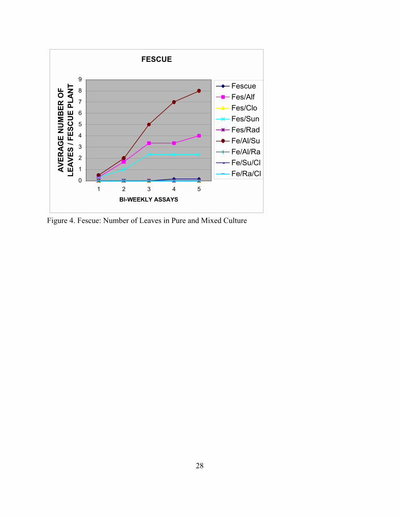
after week 4 (Figure 3). Fescue had a low rate of survival. The combinations that did survive
were combinations that contained alfalfa, sunflower, or both (Figure 4).

25
Figure 1. Alfalfa: Number of Leaves in Pure and Mixed Culture
ALFALFA
0
10
20
30
40
50
60
1 2 3 4 5
BI-WEEKLY ASSAYS
AVER
AGE
NU
MB
ER O
F LE
AVES
/ AL
FALF
A PL
ANT Alfalfa
Alf/BerAlf/FesAlf/SunAlf/RadAl/Su/BeAl/Ra/BeAl/Su/FeAl/Ra/Fe

26
Figure 2. Clover: Number of Leaves in Pure and Mixed Culture
CLOVER
0
5
10
15
20
25
30
35
1 2 3 4 5
BI-WEEKLY ASSAYS
AVER
AGE
NU
MB
ER O
F LE
AVES
/ALF
ALFA
PLA
NT Clover
Clo/BerClo/FesClo/SunClo/RadCl/Su/BeCl/Ra/BeCl/Su/Fe

27
Figure 3. Bermuda: Number of Leaves in Pure and Mixed Culture
BERMUDA
00.5
11.5
22.5
33.5
44.5
5
1 2 3 4 5
BI-WEEKLY ASSAYS
AVER
AGE
NU
MB
ER O
F LE
AVES
/ B
ERM
UD
A PL
ANT Bermuda
Ber/AlfBer/CloBer/SunBer/RadBe/Su/AlBe/Ra/AlBe/Su/ClBe/Ra/ClBe/Su/Cl
28
Figure 4. Fescue: Number of Leaves in Pure and Mixed Culture
FESCUE
0
1
2
3
4
5
6
7
8
9
1 2 3 4 5
BI-WEEKLY ASSAYS
AVER
AGE
NU
MB
ER O
F LE
AVES
/ FE
SCU
E PL
ANT Fescue
Fes/AlfFes/CloFes/SunFes/RadFe/Al/SuFe/Al/RaFe/Su/ClFe/Ra/Cl

29
Figure 5. Sunflower: Number of Leaves in Pure and Mixed Culture
SUNFLOWER
0
2
4
6
8
10
12
14
16
1 2 3 4 5
BI-WEEKLY ASSAYS
AVER
AGE
NU
MB
ER O
F LE
AVES
/ SU
NFL
OW
ER
PLAN
T
Sunflower
Sun/Alf
Sun/Clo
Sun/Ber
Sun/Fes
Sun/Alf/BerSu/Al/Fes
Su/Cl/Be
Su/Cl/Fe

30
Figure 6. Radish: Number of Leaves in Pure and Mixed Culture
RADISH
0
2
4
6
8
10
12
1 2 3 4 5
BI-WEEKLY ASSAYS
AVER
AGE
NU
MB
ER O
F LE
AVES
/ R
ADIS
H P
LAN
TRadish
Rad/Alf
Rad/Clo
Rad/Ber
Rad/Fes
Ra/Al/Be
Ra/Al/Fe
Ra/Cl/Be
Ra/Fe/Cl

31
The sunflower combinations showed the similar trends as the control group, except for the
combination with alfalfa that showed an increase and the combination with clover that showed a
decrease (Figure 5). Finally, the radish leaf number changed little between the 2nd and 5th weeks
in the control group, and between the 3rd and 5th weeks with many of the other groups (Figure 6).
Plant Biomass
Neither the number of functional groups (p =.349) nor the type of functional group
combination (p = .148) caused significant differences in aboveground biomass (Tables 5 and 6).
Belowground biomass was similarly unaffected by the number of functional groups (p = .506)
(Table 7). However, belowground biomass was marginally influenced by the type of functional
group combination (p = .066) (Table 8).
Similar amounts of plant biomass were found for total plant biomass (Figure 9) and
aboveground biomass (Figure 7). The significant variations in biomass were found in the radish
plot as a control group. Two other areas with related biomass reduction were the
alfalfa/radish/fescue and the clover/radish/fescue combinations (Figure 8). The radish plant is a
plant in which the total plant biomass is overwhelmingly controlled by belowground
components. Differences in biomass result from the ratio of above and belowground biomass for
every combination that contains the radish (Figure 9). Total plant biomass, aboveground
biomass, and belowground biomass of both individual functional group plots and of the
combined functional group plots are shown in Figures 7, 8, and 9. A presentation of the unique
functional group combinations by plot numbers is presented in Table 9.
The number of functional groups (p = .318) caused no significant difference in the total plant biomass (Table 10). However, the type of functional combination (p = .002) resulted in a

32
Table 5. Results of One-way ANOVA to Test the Effect of Number of Functional Groups on Aboveground Dry-weight Biomass. Source DF SS MS F P Number of 2 271 136 1.11 0.349 Functional Groups Error 22 2698 123 Total 24 2969
Table 6. Results of One-way ANOVA to Test the Effect of Type of Functional Combination on Aboveground Dry-weight Biomass.
Source DF SS MS F P Type of 6 1128 188 1.84 0.148 Functional Combination Error 18 1841 102 Total 24 2969

33
Table 7. Results of One-way ANOVA to Test the Effect of Number of Functional Groups on Belowground Dry-weight Biomass.
Source DF SS MS F P Number of 2 23.4 11.7 0.70 0.506 Functional Groups Error 22 366.7 16.7 Total 24 390.1
Table 8. Results of One-way ANOVA to Test the Effect of Type of Functional Combination on Belowground Dry-weight Biomass.
Source DF SS MS F P Type of 6 175.4 29.2 2.45 0.066 Functional Combination Error 18 214.7 11.9 Total 24 390.1

34
Table 9. Growth Pot Combinations. Pot # Combination Functional
type 1 ALFALFA Legume 2 CLOVER Legume 3 BERMUDA Grass 4 FESCUE Grass 5 SUNFLOWER Forb 6 RADISH Forb 7 ALFALFA/BERMUDA Leg/Gra 8 ALFALFA/FESCUE Leg/Gra 9 CLOVER/BERMUDA Leg/Gra 10 CLOVER/FESCUE Leg/Gra 11 ALFALFA/SUNFLOWER Leg/For 12 ALFALFA/RADISH Leg/For 13 CLOVER/SUNFLOWER Leg/For 14 CLOVER/RADISH Leg/For 15 BERMUDA/SUNFLOWER Gra/For 16 BERMUDA/RADISH Gra/For 17 FESCUE/RADISH Gra/For 18 FESCUE/SUNFLOWER Gra/For 19 ALFALFA/RADISH/BERMUDA Leg/For/Gra 20 SUNFLOWER/ALFALFA/FESCUE Leg/For/Gra 21 ALFALFA/RADISH/FESCUE Leg/For/Gra 22 CLOVER/RADISH/BERMUDA Leg/For/Gra 23 CLOVER/SUNFLOWER/BERMUDA Leg/For/Gra 24 CLOVER/FESCUE/SUNFLOWER Leg/For/Gra 25 CLOVER/RADISH/FESCUE Leg/For/Gra

35
Table 10. Results of One-way ANOVA to Test the Effect of Number of Functional Groups on Total Dry-weight Biomass.
Source DF SS MS F P Number of 2 326 163 1.21 0.318 Functional Groups Error 22 2965 135 Total 24 3291

36
significant difference in the total plant biomass (Table 11a). Of the 7 possible functional
combinations, the Legume-only type (L) had significantly lower biomass than either the
Legume/Grass (L/G) or Forb (F) types (Table 11b). Obviously, genetically larger plants can
acquire more biomass than genetically smaller plants, but a closer examination of Figures 7,8,
and 9 highlights the differences of particular functional combinations. Some combinations are
merely an average between the biomass of the 3 or 3 component species in the mixture. In some
cases, the largest species appeared unimpacted by neighbors as exemplified by the fact that the
clover and sunflower, bermuda and sunflower, and the fescue and sunflower combinations� total
aboveground biomass is at the same height as the sunflower alone. In contrast, both the bermuda
and fescue showed a large increase over their control plots when combined with the radish
(Figure 7).
Functional Group Variance
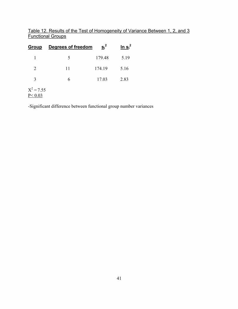
Final analyses of variance linked to functional group number indicated that stability was
gained through increasing the number of functional groups. A comparison between 1, 2, and 3
functional groups showed a significant difference (p< 0.03), and the variances associated with
increased functional group number declined (Table 12). The variance of 3 groups was
significantly lower than the variance of either 1 group (p< 0.01) or 2 groups (p< 0.01), but there
was no significant difference between 1 and 2 functional groups (p= 0.99). In addition, figure 10
shows individual variances and standard errors to relate stability to increased functional group
number.

37
Table 11a. Results of One-way ANOVA to Test the Effects of Type of Functional Combination on Total Dry-weight Biomass. Source DF SS MS F P Type of 6 2116.4 352.7 5.41 0.002 Functional Combination Error 18 1174.5 65.3 Total 24 3290.9
11b. A Posteriori (Tukey�s) Test to Show the Location of Differences Associated with the One-way ANOVA. TYPE OF COMBINATION: L/F F G/F L/G/F L/G G L
MEAN: 29a 27a 19ab 12ab 11ab 11ab 0.9b
- L(legume), G(grass), F(forb). - Means followed by different superscripts are significantly different.

38
Figure 7. Total Aboveground Dry-weight Biomass per Number of Functional Groups
TOTAL ABOVEGROUND BIOMASS
0
5
10
15
20
25
30
35
40
FUNCTIONAL COMBINATIONS1 GROUP 2 GROUPS 3 GROUPS
DYR
-WEI
GH
T B
IOM
ASS
(GR
AM
S)
ACBFSR
A/BA/FC/BC/FA/SA/RC/SR/CB/SB/RF/RS/F
A/R/BS/A/FA/R/FC/R/BC/S/BC/F/SC/R/F

39
Figure 8. Total Belowground Dry-weight Biomass per Number of Functional Groups
TOTAL BELOWGROUND BIOMASS
0
2
4
6
8
10
12
14
FUNCTIONAL COMBINATIONS1 GROUP 2 GROUPS 3 GROUPS
DRY-
WEI
GHT
BIO
MAS
S (G
RAM
S)A
C
B
F
S
R
A/B
A/F
C/B
C/F
A/S
A/R
C/S
R/C
B/S
B/R
F/R
S/F
A/R/B
S/A/F
A/R/F
C/R/B
C/S/B
C/F/S
C/R/F

40
Figure 9. Total Dry-weight Biomass per Number of Functional Groups
TOTAL BIOMASS
0
5
10
15
20
25
30
35
40
45
FUNCTIONAL COMBINATIONS1 GROUP 2 GROUPS 3 GROUPS
DRY-
WEI
GHT
BIO
MAS
S (G
RAM
S)ACBFSR
A/BA/FC/BC/FA/SA/RC/SR/CB/SB/RF/RS/F
A/R/BS/A/FA/R/FC/R/BC/S/BC/F/SC/R/F
41
Table 12. Results of the Test of Homogeneity of Variance Between 1, 2, and 3 Functional Groups Group Degrees of freedom si
2 ln si2
1 5 179.48 5.19 2 11 174.19 5.16 3 6 17.03 2.83 X2 = 7.55 P< 0.03 -Significant difference between functional group number variances

42
Figure 10. Mean Biomass per Number of Functional Groups (+/- SEM)
MEAN BIOMASS PER NUMBER OF FUNCTIONAL GROUPS
0.00
5.00
10.00
15.00
20.00
25.00
30.00
NUMBER OF FUNCTIONAL GROUPS1 2 3
BIO
MAS
S (G
RAM
S)

43
CHAPTER 4
DISCUSSION
Classroom Adventures
An effective biology classroom is one in which students learn by participating in different
activities. The best classroom adventures would include many subtopics that build on a larger
common educational goal. As the shifts in subtopics proceed, students will be able to gain the
experience of a researcher not only through learning biology but also by applying mathematics,
statistics, data collection, and writing. Biological research and the scientific method are based on
answering a question, and for the beginning student peripheral knowledge and experience is
gained during the research project. Research projects are able to give students a discovery
process because the experience is theirs (Henton 1996).
Along with the individual quest for knowledge and experience, students need to be able to
work in a group and understand that there are many different types of opinions and unique ideas.
In a society full of star athletes and a need to be the best, we sometimes forget that one idea is
not the best, rather a combination of parts of many different ideas may create the most accurate
answer. Similarly, scientific knowledge results from an accumulation and synthesis of diverse
ideas and experiences. Group involvement may also assist students with skills that will help
them mature into more outgoing and confident people. Small groups are able to strengthen skills
related to active learning such as talking, listening, reading, writing, and reflecting (Meyers and
Jones 1993). From this type of research approach, active learning will be achieved through the
experiments and the interaction with peers.
44
Methods
The planning behind this experiment on functional diversity included active learning and
group participation. Biology is a subject that can easily be used in an active learning classroom.
This research project was designed to excite the student with a topic that is both current and a
subject of considerable debate between opposing views among conservation biologists. The
concept of functional diversity is easily understood and can be related to many aspects of a
student�s life and thought processes. Some students have difficulty relating some subjects and/or
topics to their present or future lives, but functional diversity relates to 1 aspect of all lives:
eating. Students will be able to relate to the need for food as well as the impact that the
increasing world population will have on the requirement for better farming methods. Mixtures
encompassing functional diversity have already been used to double rice yields and nearly
eliminate devastating rice diseases in China, remarkably without using chemical treatments or
extra money (Yoon, 2000). Active learning is used as the students gain knowledge through
actively setting the experiment up, collecting data, analyzing data, and presenting results.
The proposed classroom project places students into research teams that interact over a period
of months. There will be 3 teams (Team 1: 1 functional group; Team 2: 2 functional groups; and
Team 3: 3 functional groups). Using teams will give the opportunity to enhance organization,
generate a wider range of ideas, and build teamwork. There are many different kinds of
�intelligence�: some students are good at writing; some are good at mathematics; while others
are good with computers or organization. A research project that involves the scientific method
allows a group of students to bring their better qualities together, and helps other students to
learn from others whose strengths differ. The scientific method involves answering questions

45
and allows the use of other skills including; organization, writing, mathematics, computer,
library, and other important skills.
At the end of the growing process, each group will be able to present information in it�s
unique way. This could be a first encounter with the scientific method for many students, and
the teacher would need to assist the students with creating testable ideas and answerable
questions. Questions have to come from some observation gained through nature or past studies.
1 question that relates to many recent studies is; does the number of species or the number of
functional groups produce more biomass? Another question could cover functional composition,
and concern the number of functional groups or the type of functional combination in regards to
biomass. Most classrooms do not have the option of visiting research sites or setting up large or
lengthy experiments, so current papers will be a good start. Finally, the ideas and hypotheses
created from the questions need to be testable within the bounds of a classroom. As we move
into experimental designs, students need to be accustomed to basic design features, which
include experimental groups, control groups, replication, and the experimental variable being
tested. Examples used with the functional diversity experiment are simple and easy to use.
Growth Area
An outdoor growth area, used initially for the development of this experiment, is an option,
depending on the soil conditions, confidence in transplantation, availability for weed removal,
and nutrient attention. The area that was used for the 2nd testing phase of the experiment was a
large growth chamber with automatic settings for light and temperature (Table 2). In a
classroom without a growth chamber, a large table and a windowsill will work for the growth
area. The use of items that are available to students at home could lead to a discussion about

46
early researchers who had only limited and simple research tools. Extra credit could be given to
students who would be willing to grow replicates at home under similar environmental
conditions as those in the classroom.
Data Collection
The data collection process has been designed in a manner that allows students to collect and
observe plants during the growth phase and also at the end of the experiment. Having collection
times during the growth phase helps keep students engaged throughout the experiment.
Observations can be conducted weekly. Plant vigor indicators such as leaf number, length of the
largest leaf blade, and shoot height can be plotted over time to show developmental trends.
Tracking trends may help students appreciate significant differences that arise from further
analysis. In addition to the importance that the timed observations give to uncovering trends,
they also keep the student actively participating in the project. Watering will have to been done
every 2 to 3 days and it is a routine task that does not require much mental involvement yet does
incorporate the responsibilities behind research methods. Weekly measurements will take about
10 to 20 minutes per student, which gives students a closer identity to their individual plants and
to the project as a whole.
The final data collection process requires more precision and patience from the students than
the weekly measurements. The teacher will need to show the students in a detailed manner the
process behind removing aboveground biomass, paying careful attention to the removal of soil
from belowground biomass. This final data collection of the experiment should have been
discussed throughout, and the younger students should know that careful attention is needed.
The aboveground removal is an easy step that only requires the cutting of the aboveground

47
biomass at the soil level. The belowground removal requires more attention and patience
because the roots will break easily. Containment of the plants in plastic bags is simple and
cheap. Bag number correlates to the group number obtained early in the project, lessening
confusion.
Aboveground and belowground wet weight measurements can be taken to assess the drastic
differences between the wet and dry weight of plants, giving students an idea of how much water
is inside a plant. Weighing of the wet plants is also good practice for the final dry weighing of
the plants. Wet weighing does not require removal of the plant from the plastic bag, as the bag is
included when taring the balance prior to the weighing procedure. Dry weighing is more time
consuming because plants must be dried in an oven. If a drying oven is not available, then
drying can be accomplished by leaving the plants in a press for a more extended amount of time
or a kitchen oven.
Showing students the process of pressing and drying plants allows the teacher to present
another activity of importance to biological research. Some students may become interested in
plant collection and choose to make it an ongoing activity. During the drying process, the plants
will have been labeled with a number on the newspaper beside the plant. Weighing the dry
plants can be done with the same balances as before. The plants will be out of the plastic bags
from the drying process, and the placement of the plants back into the bags would be a good idea
so the plants may be used for any future analyses.
Data Presentation
Data presentation is the final aspect of the scientific method, and there are many ways to
analyze and present data. Students who have just started high school may be unfamiliar with

48
statistical methods. Therefore, a statistical analysis is optional, depending on the age group and
grade level of the class. The teacher should present some basic forms of statistical analysis such
as comparing means, standard deviations, standard errors of the mean, and speak of their
importance. ANOVAS should be avoided for classes that have not learned about them.
Graphical analysis is an important aspect to science investigations, and a graphical presentation
should be included in all student reports because they efficiently convey results.
Data can be presented in a variety of different ways depending upon grade level and student
skills. Graphic, verbal and statistical analyses can be tailored to the students� level. Computers
may also assist the student. Graphs of weekly growth measurements, wet
aboveground/belowground/total biomass, and dry aboveground/belowground/total biomass all
need to be included in the analyses to observe trends related to the functional number or the
functional combination.
Functional Group Number
The 1st factor considered in the results was; Does the number of functional groups impact
total biomass? This question represents a modern perspective on species diversity. The role of
functional diversity, is 1 of the 2 aspects of biodiversity that distinguishes opposing sides of the
current controversy in conservation biology. The data produced from this experiment showed
the number of functional groups in a sample plot does not lead to differences on ecosystem
productivity or sustainability. There were no significant differences between the aboveground,
belowground, or the combined plant biomass when comparing the numbers of functional groups.
49
Functional Group Combinations
The 2nd factor considered relates to varying types of functional group combinations in a
biological community. This factor is also a leading part of the argument for maintaining
functional diversity. Particular functional combinations may have evolved to work together,
while other possibly positive combinations that are set apart by genetic, physical, or
environmental barriers may never combine without human intervention. Many future research
projects await defining and identifying functional groups and experimentation with different
combinations of the functional groups.
Is there a difference in biomass from unique combinations of functional groups? In this
experiment there were significant differences in the type of functional group combinations. The
total plant biomass showed higher significant differences in the Grass/Forb, Legume/Grass/Forb,
Legume/Grass, and Grass combinations. The belowground biomass showed a marginally
significant difference, but the aboveground did not. Special attention needs to be paid to the fact
that both the aboveground and belowground were not significantly impacted by functional
combinations, but the total biomass was. A likely reason underlying this difference is that the
ratios of aboveground and belowground biomass are different between the plant species used.
Radish plants have a huge belowground biomass in comparison to their aboveground biomass,
while sunflowers are the opposite. Difference between the radish and the sunflower present
differences between the forb group�s species. Students will need to understand that these are
early-stages in the defining of functional groups and that their ideas can be used in the search for
more defining characteristics. This adds to the inquiry-based process behind the experiment.

50
Less Variance, More Stability
In addition to the biomass assays, a final analysis was directed toward the expectation that
there will be less plot-to-plot variance in more stable communities. Therefore, variation can be
used as an indicator of stability. A simple Bartlett�s test comparing the variance between 1, 2,
and 3 functional groups revealed that there was more stability with increasing numbers of
functional groups. We may expect communities to maintain a more constant level of
productivity as functional groups are added (Figure 10).
Concluding Remarks
The need for new and innovative teaching methods grows constantly. The way that students
learn is related to the changing times and their attitudes toward education. Educators need to
focus on the minds and environments of students as well as involving them in active learning.
Teachers may not be able to make students interested in every aspect of their educational goals,
but we can attempt to introduce students to different types of learning techniques: writing,
computers, experimenting, talking, mathematical analysis, etc. Along with new innovative
techniques, there are past methods that may work for students such as memorization and
extensive lecturing. A teacher is not just a presenter of information, but a psychologist, an
inventor, and most importantly, a person who believes that the student can learn through various
strategies. This project attempts to aid students in answering a current and ongoing argument in
the field of conservation biology. Many students enjoy a good argument as much as they love
challenging authority, so the topic suits teenage personalities. Beyond this there is an interactive
system that allows the students to work in dynamic groups. This provides the students with

51
skills that they will use in a working society, on an athletic team, or at home. Grouping also
enables teachers to focus on smaller groups instead of 20 to 25 students at a time.
Using the scientific method is an integral aspect of the project. Students have the opportunity
to use and understand how this method can be adapted in their coursework in biology and other
classes. Reading recent studies will give the students some suggestions by which they may learn
how others use the scientific method. Students can create their own hypothesis prior to their own
attempt. The set up by which the hypotheses can be tested is also related to recent studies, and it
is simple enough for beginner students to understand. Results from the experiment may vary for
different classrooms, and the results will require methods for analysis.
If the students stick to using graphs for analysis, the weekly measurements will be a good
start in finding trends in the data (Figures 4-10). Figure 10 represents the mean amount of
biomass in relation to the number of functional groups combined and represents added stability
or predictability through increased functional groups. The conclusion that stability and
predictability of the system is strengthened is derived from a demonstration that the standard
error is reduced. Recent studies have also found similar results (Lehman and Tilman 2000). The
graphs on plant biomass are important for analysis because they represent biomass differences
from unique functional combinations of all species together (Figures 1-3). Other combination
differences are found in graphs, which represent all the different types of plant mixtures based on
the comparison of one individual species (Figure 11). These graphs can be broken down into
aboveground and belowground biomass (Figures 11-12). Other figures can be produced to
represent other species� combinations. These 2 figures show trends related to radish growth with
varying numbers of functional groups. Belowground biomass has better biomass production
when in 3 functional groups (Figure 12). Aboveground biomass production follows similar
trends, yet contains an increase with grass combinations (Figure 11). Students should
accomplish a comparison of other combinations. If the classes are ready for statistics, then a

52
statistical analysis discussion based on means, standard deviations, standard errors of the mean,
t-tests, and ANOVAS will be appropriate for use. These steps to the scientific method are
pertinent to know in the field of biology, as the scientific method is discussed in several high
school biology classrooms and in all college level courses including ecology, genetics,
biochemistry, and conservation biology. The above courses can be combined or used separately
in an attempt to identify functional roles of plant species and combinational effects.

53
BIBLIOGRAPHY
Hector, A. 1999. Plant diversity and productivity experiments in European grasslands. Science 286: 1123-1127. Henton, M. 1996. Adventures in the Classroom. Kendall/Hunt Publishing Company, Dubuque, Iowa. Lehamn, C., and D. Tilman. 2000. Biodiversity, stability, and productivity in competitive communities. American Naturalist 156: 534-551. Loreau, M., S. Naeem, P. Inchausti, J. Bengtsson, J. P. Grime, A. Hector, D. U. Hooper, M. A.
Huston, D. Raffaelli, B. Schmid, D. Tilman, and D.A. Wardle. 2001. Biodiversity and ecosystem functioning: current knowledge and future challenges. Science 294. 804-808.
Lyons and Swarts. 2001. Contributions large and small. Science 293: 1017. Meffe, G. K., C. R. Carroll., and Contributors. 1997. Principles of Conservation Biology, Second
Edition. Sinauer Associates, Inc. Publishers, Sunderland, Massachusetts. Meyers, C., and T. Jones. 1993. Promoting Active Learning. Jossey-Bass Publishers, San Fransisco. Naeem, S., and S. Li. 1997. Biodiversity enhances ecosystem reliability. Nature
390: 507-509. Naeem, S., L. J. Thompson, S. P. Lawler, J. H. Lawton and R. M. Woodfin. 1994.
Declining biodiversity can alter the performance of ecosystems. Nature 368: 734-737. National Research Council. 1992. Conserving biodiversity. National Academy Press, Washington, D.C. Tilman, D., J. Knops, D. Wedin, P. Reich, M. Ritchie, and E. Siemann. 1997. The influence of functional diversity and composition on ecosystem processes.
Science 277: 1300-1302. Tilman, D., P. Reich, J. Knops, D. Wedin, T. Mielke and C. Lehman. 2001. Diversity and
productivity in a long-term grassland experiment. Science 294: 843-845. Wilson, E. O. 1984. Biophilia. Harvard University Press, Cambridge, Mass. Yoon, C. K. 2000. Simple method found to increase crop yields vastly. The New York
Times/Science. Tuesday, August 22.

54
APPENDICES

55
APPENDIX A
Lesson Plans for an Inexpensive Experiment on Functional Diversity
Day 1. * Discuss the scientific method. * Discuss Biodiversity (the variety of organisms on the planet). * Ask students to explain Biodiversity in their own words (groups of 4). * Talk about current events and studies surrounding Biodiversity. * Present a movie concerning biodiversity to excite the students. * (Homework) Have students bring in a picture and description of their favorite organism(s). Day 2. * Discuss homework. * Introduce concept of functional diversity. * Compare and contrast functional diversity and biological or species diversity. * Describe possible functions of the students� chosen organisms. * Explain different functions already identified (nitrogen-fixation, strong roots, allelopathy, etc.). * Assign previously identified functions to students and have them combine their functions in a manner that could be positive for the environment. * Ask students to explain why certain combinations would and would not be expected to work. * Search for other plant characteristics that would be considered as different functions (current topic). * Discuss the first and second parts of the scientific method (observation and asking questions). * Ask the class what they observe about biological and/or functional diversity and have them think of questions from the observations. * Explain the reasons for doing the experiment and the questions being asked. * (Homework) Write in your own words a comparison/contrast of functional and biological diversity. Ask some questions that arise concerning the topic. Day 3. * Discuss homework. * Have the class discuss their own experimental approach. * Discuss the experimental variable, control group, experimental group, constants, and types of comparisons. * Present the design used in this study. * Prepare to plant the seeds on Day 4. * Assign students their individual functional combination and combination number. * Pass out and explain data sheets (attachment B). * Explain the phenotypic characters to measure (shoot height, leaf number, and largest leaf blade).
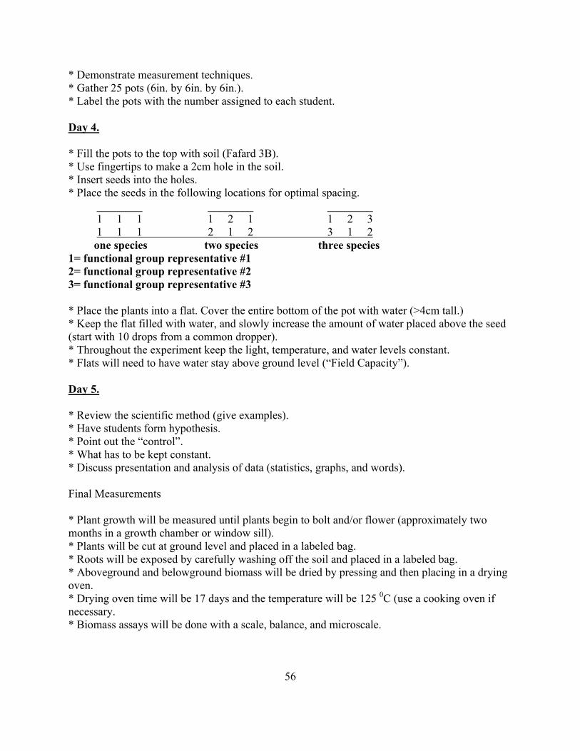
56
* Demonstrate measurement techniques. * Gather 25 pots (6in. by 6in. by 6in.). * Label the pots with the number assigned to each student. Day 4. * Fill the pots to the top with soil (Fafard 3B). * Use fingertips to make a 2cm hole in the soil. * Insert seeds into the holes. * Place the seeds in the following locations for optimal spacing. ________ ________ ________ 1 1 1 1 2 1 1 2 3 1 1 1 2 1 2 3 1 2 one species two species three species 1= functional group representative #1 2= functional group representative #2 3= functional group representative #3 * Place the plants into a flat. Cover the entire bottom of the pot with water (>4cm tall.) * Keep the flat filled with water, and slowly increase the amount of water placed above the seed (start with 10 drops from a common dropper). * Throughout the experiment keep the light, temperature, and water levels constant. * Flats will need to have water stay above ground level (�Field Capacity�). Day 5. * Review the scientific method (give examples). * Have students form hypothesis. * Point out the �control�. * What has to be kept constant. * Discuss presentation and analysis of data (statistics, graphs, and words). Final Measurements * Plant growth will be measured until plants begin to bolt and/or flower (approximately two months in a growth chamber or window sill). * Plants will be cut at ground level and placed in a labeled bag. * Roots will be exposed by carefully washing off the soil and placed in a labeled bag. * Aboveground and belowground biomass will be dried by pressing and then placing in a drying oven. * Drying oven time will be 17 days and the temperature will be 125 0C (use a cooking oven if necessary. * Biomass assays will be done with a scale, balance, and microscale.

57
APPENDIX B
Data Table for Bi-weekly Analyses
Plant ID #
ID germination date
leaf number
shoot height
Length of largest blade
aboveground biomass
belowground biomass
1a A 1b A 1c A 1d A 1e A 1f A 2a C 2b C 2c C 2d C 2e C 2f C 3a B 3b B 3c B 3d B 3e B 3f B 4a F 4b F 4c F 4d F 4e F 4f F 5a S 5b S 5c S 5d S 5e S 5f S 6a R 6b R

58
Data Table for Bi-Weekly Analyses
Plant ID #
ID germination date
leaf number
shoot height
Length of largest blade
aboveground biomass
belowground biomass
6c R 6d R 6e R 6f R 7a A 7b B 7c A 7d B 7e A 7f B 8a A 8b F 8c A 8d F 8e A 8f F 9a C 9b B 9c C 9d B 9e C 9f B 10a C 10b F 10c C 10d F 10e C 10f F 11a A 11b A 11c S 11d A 11e S 11f S 12a A 12b R 12c A

59
Data Table for Bi-weekly Analyses Plant ID #
ID germination date
leaf number
shoot height
length of largest blade
aboveground biomass
belowground biomass
12d R 12e A 12f R 13a C 13b S 13c C 13d S 13e C 13f S 14a C 14b R 14c C 14d R 14e C 14f R 15a B 15b S 15c B 15d S 15e B 15f S 16a F 16b S 16c F 16d S 16e F 16f S 17a B 17b R 17c B 17d R 17e B 17f R 18a F 18b R 18c F 18d R

60
Data Table for Bi-weekly Analyses Plant ID #
ID germination date
leaf number
shoot height
length of largest blade
aboveground biomass
belowground biomass
18f R 19a F 19b S 19c F 19d S 19e F 19f S 20a A 20b A 20c R 20d R 20e B 20f B 21a A 21b A 21c S 21d S 21e F 21f F 22a A 22b A 22c R 22d R 22e F 22f F 23a C 23b C 23c S 23d S 23e B 23f B 24a C 24b C 24c R 24d R 24e B

61
Data Table for Bi-weekly Analyses Plant ID #
ID germination date
leaf number
shoot height
Length of largest blade
aboveground biomass
belowground biomass
25a C 25b C 25c S 25d S 25e B 25f B 26a C 26b C 26c S 26d S 26e F 26f F 27a C 27b C 27c F 27d F 27e R 27f R

62
VITA
CORY M. STANLEY
Personal Data: Date of Birth: March 31, 1977 Place of Birth: Brevard, North Carolina Marital Status: Single Education: Public Schools, Brevard, North Carolina Mars Hill College, Mars Hill, North Carolina;
Biology, B.S., 1999 East Tennessee State University, Johnson City, Tennessee;
Biology, M.S., 2002 Professional Experience: Graduate Teaching Assistant, East Tennessee State University, College of
Biological Sciences, 1999 � 2002 .