An Experimental Evaluation of Constrained ApplicationProtocol Performance over TCP

Laura Pesola

Helsinki January 30, 2020

Master’s thesis

UNIVERSITY OF HELSINKIDepartment of Computer Science

Faculty of Science Department of Computer Science

Laura Pesola

An Experimental Evaluation of Constrained ApplicationProtocol Performance over TCP

Computer Science

Master’s thesis January 30, 2020 75 pages

CoAP, TCP, CoAP over TCP, congestion control, IoT protocols, performance analysis

The Internet of Things (IoT) is the Internet augmented with diverse everyday and industrial objects,enabling a variety of services ranging from smart homes to smart cities. Because of their embeddednature, IoT nodes are typically low-power devices with many constraints, such as limited memoryand computing power. They often connect to the Internet over error-prone wireless links with lowor variable speed. To accommodate these characteristics, protocols specifically designed for IoT usehave been designed.

The Constrained Application Protocol (CoAP) is a lightweight web transfer protocol for resourcemanipulation. It is designed for constrained devices working in impoverished environments. Bydefault, CoAP traffic is carried over the unreliable User Datagram Protocol (UDP). As UDP is con-nectionless and has little header overhead, it is well-suited for typical IoT communication consistingof short request-response exchanges. To achieve reliability on top of UDP, CoAP also implementsfeatures normally found in the transport layer.

Despite the advantages, the use of CoAP over UDP may be sub-optimal in certain settings. First,some networks rate-limit or entirely block UDP traffic. Second, the default CoAP congestion controlis extremely simple and unable to properly adjust its behaviour to variable network conditions, forexample bursts. Finally, even IoT devices occasionally need to transfer large amounts of data, forexample to perform firmware updates. For these reasons, it may prove beneficial to carry CoAPover reliable transport protocols, such as the Transmission Control Protocol (TCP). RFC 8323specifies CoAP over stateful connections, including TCP. Currently, little research exists on CoAPover TCP performance.

This thesis experimentally evaluates CoAP over TCP suitability for long-lived connections in aconstrained setting, assessing factors limiting scalability and problems packet loss and high levelsof traffic may cause. The experiments are performed in an emulated network, under varying levelsof congestion and likelihood of errors, as well as in the presence of overly large buffers. For TCPresults, both TCP New Reno and the newer TCP BBR are examined. For baseline measurements,CoAP over UDP is carried using both the default CoAP congestion control and the more advancedCoAP Simple Congestion Control/Advanced (CoCoA) congestion control.

This work shows CoAP over TCP to be more efficient or at least on par with CoAP over UDP in aconstrained setting when connections are long-lived. CoAP over TCP is notably more adept thanCoAP over UDP at fully utilising the capacity of the link when there are no or few errors, evenif the link is congested or bufferbloat is present. When the congestion level and the frequency oflink errors grow high, the difference between CoAP over UDP and CoAP over TCP diminishes, yetCoAP over TCP continues to perform well, showing that in this setting CoAP over TCP is morescalable than CoAP over UDP. Finally, this thesis finds TCP BBR to be a promising congestioncontrol candidate. It is able to outperform the older New Reno in almost all explored scenarios,most notably in the presence of bufferbloat.

ACM Computing Classification System (CCS):Networks → Network performance evaluationNetworks → Application layer protocolsNetworks → Cross-layer protocolsNetworks → Transport protocols

Tiedekunta — Fakultet — Faculty Laitos — Institution — Department

Tekijä — Författare — Author

Työn nimi — Arbetets titel — Title

Oppiaine — Läroämne — Subject

Työn laji — Arbetets art — Level Aika — Datum — Month and year Sivumäärä — Sidoantal — Number of pages

Tiivistelmä — Referat — Abstract

Avainsanat — Nyckelord — Keywords

Säilytyspaikka — Förvaringsställe — Where deposited

Muita tietoja — övriga uppgifter — Additional information

HELSINGIN YLIOPISTO — HELSINGFORS UNIVERSITET — UNIVERSITY OF HELSINKI

ii

Contents

1 Introduction 1

2 Communication In The Internet of Things 3

2.1 Internet of Things . . . . . . . . . . . . . . . . . . . . . . . . . . . . . 3

2.2 Constrained Application Protocol (CoAP) . . . . . . . . . . . . . . . 7

2.3 CoAP over TCP . . . . . . . . . . . . . . . . . . . . . . . . . . . . . 10

3 Congestion Control 13

3.1 Congestion . . . . . . . . . . . . . . . . . . . . . . . . . . . . . . . . . 13

3.2 TCP Congestion Control . . . . . . . . . . . . . . . . . . . . . . . . . 15

3.3 CoAP Congestion Control . . . . . . . . . . . . . . . . . . . . . . . . 21

3.4 Alternatives to CoCoA . . . . . . . . . . . . . . . . . . . . . . . . . . 26

4 Experiment Setup 29

4.1 Experiment Design and Workloads . . . . . . . . . . . . . . . . . . . 29

4.2 Network Setup and Implementation Details . . . . . . . . . . . . . . . 31

4.3 Metrics . . . . . . . . . . . . . . . . . . . . . . . . . . . . . . . . . . . 34

5 Related Results 35

5.1 CoAP over UDP . . . . . . . . . . . . . . . . . . . . . . . . . . . . . 35

5.2 CoAP over TCP for Short-Lived Connections . . . . . . . . . . . . . 38

6 CoAP over TCP in Long-Lived Connections 43

6.1 Error-Free Link Results . . . . . . . . . . . . . . . . . . . . . . . . . . 43

6.2 Error-Prone Link Results . . . . . . . . . . . . . . . . . . . . . . . . . 51

6.3 Summary . . . . . . . . . . . . . . . . . . . . . . . . . . . . . . . . . 66

7 Conclusion 68

References 70

1

1 Introduction

The Internet of Things, in a very broad sense, means the augmentation of theInternet with nodes other than traditional computers and smartphones [XQY16].These diverse physical objects are equipped with electronics and software that allowthem to communicate with each other, and to integrate with the existing Internetinfrastructure [RJR16, AIM10, XQY16]. A wide variety of services ranging fromhealthcare and social networking to smart homes, smart factories, and even smartcities can be built using these devices [AIM10]. Relatedly, IoT devices differ innumerous ways—for example, in their traffic patterns and where they are located.

Typical for IoT devices—regardless of whether they are simple sensors or morecomplicated objects—is their small size and limited availability of resources such asenergy, CPU, and memory. IoT devices also often fit the definition of a constraineddevice [BEK14]. A network formed by constrained devices is typically a low-poweredlossy network [Vas14] or a constrained network where a low bit rate and high errorrate cause problems such as congestion and frequent packet loss [BEK14]. Thecharacteristics of such networks challenge the assumptions made in the Internet oftoday, rendering the current Internet protocols suboptimal for IoT traffic [RJR16],leading to a need for more suitable protocols.

The Constrained Application Protocol (CoAP) [SHB14] is a lightweight web trans-fer protocol for resource manipulation for constrained devices in impoverished en-vironments. It is a simple protocol with low overhead, suitable for machine to ma-chine communication. CoAP operates using a request-response model, much like theHyper-Text Transfer Protocol [FR14], which it is modelled after. The two can easilybe used together, but CoAP also differs from HTTP. The most important differenceis that CoAP implements features typically found in the transport layer such asreliability and congestion control. However, the congestion control in CoAP is verystraightforward and cannot take into account the conditions of the network: it isunable to adapt to, for example, fluctuations in connection speed. This makes CoAPcongestion control ill-suited for handling sudden changes such as bursts [BGDP16].These drawbacks have motivated the work on new, more adaptive and efficient con-gestion control mechanisms for CoAP. The most established of these alternativesis the CoAP Simple Congestion Control/Advanced (CoCoA) [BBGD18] which hasbeen shown to outperform the Default CoAP congestion control [BGDP16, JDK15,BGDP15, BGDK14, BGDP13, BKG13]. In addition to CoCoA, other new andexisting congestion control mechanisms have been studied in constrained settings.These include, for example, the Peak Hopper [BGDP16, JDK15] and the LinuxRTO [BGDP16, BGDP13] retransmission timeout algorithms, as well the more com-plex congestion control algorithms such as CoCoA 4-state-strong [BSP16] and therecent FASOR RTO and congestion control mechanism for CoAP [JRCK18a].

By default, CoAP operates over the User Datagram Protocol, UDP [Pos80], whichis well-suited to resource-restricted environments due to its minimal headers andconnectionless communication model. While the choice has its benefits, it can alsoprove problematic as there are networks that do not forward UDP traffic [BLT+18].

2

Certain networks may also rate-limit [BK15] or completely block it [EKT+16]. Fur-ther, even though CoAP traffic most typically consists of only intermittent request-response pairs, sometimes large amounts of data need to be transferred as well,for example to perform firmware updates. In these kinds of situations it might benecessary to carry CoAP traffic over a reliable protocol such as the TransmissionControl Protocol, TCP [Pos81]. CoAP over TCP, TLS, and WebSockets [BLT+18](RFC 8323) specifies a CoAP version suitable for use over stateful connections.As the specification is relatively new, little research currently exists. One prelimi-nary study suggests that CoAP over TCP might perform poorly compared with theDefault CoAP [ZFC16], whereas another argues many of the issues attributed tocarrying CoAP over TCP could also be easily solvable or not very consequential atall [GAMC18]. The scope of these studies is limited and their results inconclusive,motivating the need for further research.

This work experimentally evaluates the performance of CoAP over TCP in an em-ulated wireless network, under diverse conditions such as in the presence of buffer-bloat [GN11], as well as varying levels of congestion and likelihood of packet losscaused by link-errors. The aim is to assess the performance of CoAP over TCP byexploring which factors limit scalability and what kind of problems high levels oftraffic and packet loss may cause. The experiments are carried out in real hosts overan emulated wireless link. For baseline measurements, UDP is used as the transportprotocol with both the Default CoAP and the CoCoA congestion controls. The cor-responding measurements are carried out using a CoAP over TCP implementationon top of TCP New Reno [HFGN12]. A subset of the experiments also employ therecent TCP BBR [CCG+16], a model-based congestion control. These key resultsare compared to the baseline measurements. The focus of this thesis is on a scenariowhere the connections are long-lived due to the large amount of data transferred.

This thesis is arranged as follows. Chapter 2 offers an overview of communicationin the Internet of Things, presenting constrained networks and their key proper-ties to motivate the design of, and the need for CoAP. Chapter 3 introduces theconcept of congestion, describes the most central TCP and CoAP congestion con-trol mechanisms in necessary detail, and shortly summarises alternative CoAP overUDP congestion controls as well as their performance. Chapter 4 describes the testenvironment and the design of the experiments of this thesis, as well as the metricsused in evaluating the results. Chapter 5 reviews other results achieved in the setupdescribed in the Chapter 4, focusing mostly in CoAP over UDP but ending with abrief overview of CoAP over TCP for short-lived connections. Chapter 6 presentsthe results of this thesis. Finally, Chapter 7 concludes this thesis.

3

2 Communication In The Internet of Things

This Chapter briefly introduces the Internet of Things and outlines the character-istics of communication in the Internet of Things. The Constrained ApplicationProtocol and its features are introduced in the extent that is needed for understand-ing the results of this thesis. The aim of this chapter is to explain and to motivateCoAP design and the need for a specific protocol for constrained devices. Morethorough portrayals of CoAP and CoAP over TCP can be found in the respectiveRequests for Comments.

2.1 Internet of Things

The Internet of Things (IoT) consists of ubiquitous physical objects—things—whichuse electronics, software, and network connectivity to enable interaction with thephysical world. These things may sense and control the physical world or they maybe remotely sensed and controlled themselves. They collect and exchange data, bothbetween themselves and with the outside world. Further, they are extremely variedin their use and nature, which range from everyday items to very specialised equip-ment [AIM10, RJR16, XQY16]. Often called edge devices, these enhanced objectstypically communicate with edge routers, which in turn connect to the Internet us-ing gateways. Edge devices may also form sub-networks consisting only, or mostly,of edge devices. Typically, the data collected by the edge devices is processed bypowerful servers in the Internet, since the edge devices lack the necessary computa-tional capacity [RJR16]. This manner of setup is illustrated in Figure 1. However,the gateways may also perform some manner of pre-treatment or other processingof the data they receive [RJR16]. The low latency achieved by performing the com-putation at the edge of the network is becoming more common as it crucial or atleast useful for many IoT applications [MNY+18].

Gateway Gateway

Edge

router Edge

routerInternet

Figure 1: Edge devices communicate with servers that process the data collected bythe edge devices. The edge devices are connected to an edge router using a low-powerlossy link, while the edge routers are connected to the Internet via gateways.

4

While useful, embedding electronics into varied physical objects poses many chal-lenges. For example, if the devices are incorporated into clothing, the electronicsused for communication must fit in very small spaces [AIM10]. Limited space meanslimited capabilities, and most IoT devices are indeed low-power [AIM10, RJR16]and have constraints on energy expenditure [RJR16]. Additionally, they sufferfrom limited available computational capacity as very advanced chips require morespace [AIM10].

A device that is limited in all its resources—CPU, memory, and power—is a con-strained device [BEK14]. Such devices may not be able to take all the same actionsthat typical modern Internet nodes can, and they may not perform as well. Forexample, if a constrained device is not mains-powered but instead needs to use bat-teries, it might need to conserve energy and bandwidth. Constrained nodes mayalso have very little Flash or read-only memory (ROM) available, inhibiting codecomplexity. Additionally, having little RAM limits the ability to store state or em-ploy buffers. Low processing power limits the amount of computation the devicesmay feasibly perform in a given time frame. As these various constraints are foundtogether, they may amplify each other’s effects.

Terminology

Constrained nodes are classified based on their capabilities [BEK14]. Class 0 devicesare severely limited, typically sensor motes. The only feasible way for them toparticipate in the Internet safely is with the help of other, more capable devices,by using proxies or other similar solutions. Class 1 devices, on the other hand, areable to employ more complex protocols. They are advanced enough to take part inan IP network as they are capable of implementing the security measures requiredfor safe usage of a large network. Still, they need to be conservative about howspace is used for code, how much they can have state, and typically also abouttheir energy usage. These limitations mean that they are too impoverished to easilyimplement the full HTTP stack. Thus, in order to communicate in the Internet,they need special protocols that take into account their limited nature [BEK14].The Constrained Application Protocol is an example of such a protocol. Finally,Class 2 devices are quite capable compared to the other two classes, and as suchmight not necessarily need a protocol specifically designed for constrained nodes.However, these devices may still benefit from using a protocol such as CoAP inorder to, for example, minimise bandwidth and energy use. Likewise, even morecapable devices might opt to employ CoAP for similar reasons.

These constraints may also limit the connectivity of the devices. Limited spacemay, for example, mean restricting the number of antennas to only one [RAVX+16],which limits network capabilities of the device. Reduced computational complex-ity may lead to a low bandwidth or few transmission modes [RAVX+16]. Theselimitations of the nodes and also the limited capability of the used link may leadto congestion [BSP16]. Limits on energy expenditure might also require that thedevice employ duty cycling, and that the cycles are kept low so that the device is

5

only active for a small portion of the time [RJR16]. Further, IoT devices commonlyemploy short-range wireless transmission technologies, which are not suitable forlong distance connections and cannot provide high speeds [XQY16]. Finally, IoTdevices typically employ wireless links that are prone to link errors [AIM10, RJR16].

In such cases, the networks might be constrained, too. A constrained network is anetwork that lacks some features and capabilities standard in the current-day In-ternet [BEK14]. Such a network might have a low throughput and its nodes maybe reachable only intermittently if they alternate between sleep and wake cycles.Further, links may be asymmetric in their operation. Larger packets are penalised.For example, fragmenting packets may cause frequent losses. A constrained networkeither does not have, or has limited, availability of advanced Internet services likemulticast. In general, packet loss may be frequent or vary greatly. These constraintsmay arise, among other things, from the constraints of the nodes themselves, en-vironmental challenges such as being operated under water, or regulations such aslimited available spectra. A constrained node network is a network which consistsmostly of constrained nodes. The constraints of the nodes affect the characteris-tics of the network. A constrained node network might suffer, for example, fromunreliable channels or it may have limited or unpredictable bandwidth, as well afrequently changing topology. A constrained node network is a constrained networkbut not all constrained networks are constrained node networks.

An often-used class of constrained networks is a Low-Power Wireless Personal AreaNetwork (LoWPAN). It is a wireless network formed by devices conforming to theIEEE 802.15.4-2003 standard that have limited power [KMS07]. The participatingdevices typically are low-cost, constrained devices, which have short range, low bitrate, limited power, and little memory. Applications used within a LoWPAN donot have to achieve a high throughput [BEK14], and indeed a LoWPAN may onlyoffer low bandwidth. Achieved data rates vary depending on the physical layer used,typically ranging from 20 kbps to 40, but even higher data rates of up to 250 kbpsmay be achieved. Another distinguishing feature is very small packet size. For thephysical layer, the maximum size is only 127 bytes, which only allows for 81 octetsof payload data, taking into account overhead such as security. Finally, the devicesin a LoWPAN may move or be deployed in an ad-hoc fashion so that they do nothave a pre-defined location [KMS07]. Despite the name, LoWPANs are suggestedfor uses such as building automation and urban and industrial monitoring. Origi-nally, LoWPAN technology was focused on IEEE 802.15.4, but it may also refer toother similar physical layer techonologies [BEK14]. Finally, another term related toconstrained networks is a Low-Power and Lossy Network (LLN) [BEK14]. An LLNalso consists of embedded devices that are constrained, using either IEEE 802.15.4or low-power Wi-Fi. Like LowPANs, LLNs are found in industrial monitoring, build-ing automation systems, and similar applications. They are prone to losses at thephysical layer, and exhibit both variable delivery rates and short-term unreliability.Notably, an LLN in reliable enough to warrant constructing directed acyclic graphsfor routing purposes [BEK14].

6

Data link layer protocols for IoT

A number of data link layer protocols are used in the Internet of Things. These in-clude both general-use cellular services as well as protocols specifically designed forIoT use. While different, these protocols share certain characteristics. For example,their wireless nature makes them more prone to link errors than wired connections.Typically they also provide low data rates compared to what is typically achievedwith wired connections in the modern day Internet. The following have been em-ployed in Constrained Application Protocol performance research [BGDP16, JDK15,BGDP15, BGDK14, BGDP13, BSP16, JRCK18a, JPR+18], but other protocols suchas SigFox, LoRa, and WiMaxb, exist as well.

Since the 1990s, cellular networks have progressed through five generations, all ofwhich have been used with IoT [LDXZ18]. The first to offer practical data transferwas the second generation (2G) General Packet Radio Service (GPRS) [Ake95]. Be-fore GPRS, data transfer in the Global System for Mobile Communications (GSM)was possible, but employed circuit-switched data bearer services, which made it veryinefficient in face of bursty Internet traffic. GPRS was standardised already in the1990s [HMS98] but is still researched and deployed in real-world scenarios, especiallyin outdoor monitoring [LNV+17, HZA19, NV19, ZW16], which is natural consider-ing it covers a significant portion of all population [LDXZ18]. The theoretical datarate for GPRS varies from few to 170 kbits [BBCM99] but actual data rates dependon error rate and whether the endpoint is stationary—a moving endpoint achievesa much lower data rate [OZH07]. Generally, the achieved data rates fall between15 and 45 kbits [FO98, HMS98, CG97, OZH07], with 30 to 40 kbps being the mosttypical [OZH07].

After GPRS, the LTE data rates have grown considerably: 3rd generation (3G)EDGE could achieve a data rate of 384 kbps [HWG09, ASHA18] while the 4thgeneration (4G) is able to achieve a rate of up to 1Gbps [LDXZ18]. Both 3Gand 4G are used widely with IoT, although they are not perfectly optimised forIoT use [LDXZ18]. For example, 4G is easily disrupted by other signals such as mi-crowaves or physical objects [ASHA18]. However, the latest in the cellular evolution,the 5th generation (5G), which is expected to be commercially available by 2020, hasbeen designed to accommodate IoT needs. While 3G and 4G mostly brought withthem increased data rates, 5G is hoped to also improve support for hotspots andwide-area coverage, mobility and high device density, as well as increased capacityand data rates of up to 10 Gbps [LDXZ18]—without sacrificing energy-efficiency orreliability [SMS+17, LDXZ18]. 5G design should be suitable for a wide range ofservices with differing needs, ranging from ultra-reliable low-latency applications toapplications with massive numbers of low-cost devices with high data-volume thatdo not have strict requirements for low latencies [SMS+17]. Due to this flexibilityand its other improvements, 5G is expected to be important in future IoT [LDXZ18].

ZigBee is typical in smart home systems [BPC+07]. The two lower layers of theZigBee protocol stack, physical and MAC layer, are defined by the IEEE 802.15.4standard while the network and the application layer are defined by the ZigBee

7

specification [GP10, MPV11]. ZigBee is developed by an association of companies,the ZigBee alliance, that develops standards and products for low-power wirelessnetworking [GP10, BPC+07]. ZigBee attempts to minimise power consumption toenable networking for devices that are not mains-powered or that, for other reasons,need to conserve energy. ZigBee supports different topologies [MPV11] and providessecurity across the network and the application layers [GP10]. Ranges achieved withZigBee depend on the number of nodes: a range for a typical node is 10 meters, butsome implementations may have a higher range of even 100 meters. As a ZigBeenetwork may contain thousands of nodes, if messages are relayed through othernodes, the ranges may grow longer [SM06]. The data rates supported by IEEE802.15.4, and as such by ZigBee, range from 20 kbps to 40 kbs, although even a rateof 250 kbps may be achieved [MPV11].

Narrowband IoT (NB-IoT) is a recent low-power, wide-area cellular technologyspecifically designed for general IoT use, accommodating the special requirementsand restrictions of IoT devices [RAVX+16, WLA+16]. NB-IoT targets low-power,non-complex, stationary devices—such as sensors—that may reuse the bands ofexisting cellular technologies, and for which low data-rate is acceptable. WhileNB-IoT is not entirely backwards compatible, it is able to coexist with legacy tech-nologies such as GPRS. NB-IoT can support numerous devices in one cell and has asignificantly extended coverage compared with the existing, older cellular technolo-gies [WLA+16]. NB-IoT reaches data rates of 50 kbps for uplink, and 30 kbps fordownlink [RAVX+16]. Theoretically, even a data rate of up to 250 kbps is achiev-able. Notably, under certain conditions, NB-IoT may also provide very low, sub10-second, latencies for critical applications such as alarms [WLA+16]. Multicastand 5G support as well as improved positioning are underway [WLA+16].

2.2 Constrained Application Protocol (CoAP)

IoT nodes are often constrained, and as such they may not be able to use protocolsthat are not designed to accommodate their limitations. The Constrained Appli-cation Protocol (CoAP) [SHB14] is specifically designed for these devices. It is alightweight RESTful [FTE+17] protocol for controlling and transferring resourcesin impoverished environments. As a web transfer protocol it is modelled after thehyper-text transfer protocol (HTTP) [FR14], and can easily be mapped to it. LikeHTTP, CoAP employs the client-server interaction model: An endpoint acting asthe client sends a request to an endpoint acting as the server. The endpoint actingas the server receives the request, attempts to act on it, and finally informs the clientof the result. During its lifetime, an endpoint may act in the role of both the clientand the server. For example, a server may query a sensor to acquire its currentreadings, and additionally the sensor may send updates to the server periodically,or as a response to an external event. A request in this model is an action the serverexecutes on a resource that typically is specified in the request. An action fetches,updates, uploads, or deletes data. Possible actions in CoAP are get, head, post, put,

8

and delete. While similar, the semantics of the actions are not exactly the same forCoAP and HTTP.

CoAP differs from HTTP in a few notable ways that make it suitable for machine-to-machine communication and constrained devices. First, CoAP is simpler andhas less overhead. Second, CoAP supports multicast and resource discovery. Third,by default, CoAP uses the unreliable UDP as its transport protocol. The choiceis sensible as UDP has less overhead than TCP that HTTP relies on, but it alsoforces CoAP to settle for the possibility of messages arriving out of order or notarriving at all—unless it implements the reliability itself. This is the final differencebetween CoAP and HTTP. CoAP is cross-layer in that it implements functionalitytraditionally found in the transport layer, including congestion control and optionalreliability. CoAP messages may be non-confirmable or confirmable. The latteroffer TCP-like reliability based on acknowledgements. All the experiments of thisthesis were carried out using the reliable confirmable messages, so the unreliablenon-confirmable messages are not discussed further.

When using confirmable messages, a new message is sent to an endpoint only afterthe acknowledgement for the previous one has been received. However, sendingmessages to other endpoints is allowed as long as the previous message to thatendpoint has already been acknowledged. This keeps the number of messages inflight decidedly low. CoAP response arriving from the server can be piggybacked inthe acknowledgement of the request if the results are immediately available, or, ifnot, sent as a separate message. A piggybacked response does not need a separateacknowledgement.

Much of the lightweight nature of CoAP is due to the short, four byte basic headershown in Table 1. It consists of the message type T, code, message id, token lengthTKL, and protocol version number Ver fields.

The types of messages in CoAP are Confirmable, Non-confirmable, Acknowledge-ment, and Reset. The first two, as discussed above, indicate whether acknowledge-ments are expected. The acknowledgement messages are used together with theConfirmable messages to indicate that the other end has received the request thatwas sent. Finally, a Reset message is sent in response to a request the other end wasnot able to process. The code field is used to mark the message as either a responseor a request. In a request, the code field also defines the action: get, post, put,or delete. In a response the code field indicates success or failure. The code field

1 2 3 4 5 6 7 8 1 2 3 4 5 6 7 8 1 2 3 4 5 6 7 8 1 2 3 4 5 6 7 8Ver T TKL Code Message IDToken, if definedOptions, if anyPayload marker Payload, if any

Table 1: The CoAP header.

9

also includes the explanatory return code for the result. The Message ID is used forduplicate detection and for matching acknowledgements and resets to the requests.

A token is used to match a response to a request. Similar to the Message ID,the token can be also be used when the response is not piggybacked. The tokenis optional. A servers echos the token set in the request so that the client mayrecognise which request the message is a response to. Considering that the headeris only four bytes, the token field may be reasonably long, up to 8 bytes. This isfor security reasons. A token is not mandatory. If not used, the token length fieldis set to 0 to indicate a zero byte token. If used, the token length field is set toa non-zero value that indicates the length of the token field, and the token itselffollows immediately after the header.

To enable further control over the communication, CoAP includes a set of options.Options may, for example, specify the path of the resource the request targets, queryproxies, specify the format of the content, or indicate the version of the resource.Some options are critical: they must not be ignored. If a CoAP endpoint does notsupport a critical option, it must reject all messages that include the option. Arange of option numbers is reserved for private and vendor-specific options. If used,they are placed after the token.

The rest of the datagram is reserved for the payload that is preceded by the payloadmarker, a 1-byte padding field. In case a message does not include any payload, itmust not include a payload marker either.

Block-Wise Transfer

Originally CoAP was designed to handle small requests and responses, and so themessaging model is not perfectly suitable for transferring larger amounts of data.To avoid IP and adaptation-layer fragmentation, the size of datagrams should staysmall. On the other hand, a small maximum datagram size limits the amount ofdata that can be transferred, if connection state cannot be tracked. To enablelarger messages within the messaging model of CoAP, a new critical CoAP option,the Block-Wise option, was introduced [BS16]. In Block-Wise Transfer, a largemessage is split into multiple parts, so-called blocks. Each block is treated as if itwas a single CoAP message. However, to the receiver the Block option indicatesthat, semantically, the message is only a part of a larger message.

The size of a block ranges from 16 to 1024 bytes: the connection ends negotiate thesize to be used. The size may be negotiated after the requesting end has received thefirst response, or, if it anticipates a Block-Wise Transfer, in the first request itself.After the block size has been negotiated, all blocks must be of the same size, exceptfor the last block which may be smaller than the previous blocks. While both endsmay express a wish to use a certain size, the specification recommends the sendingend respects the request of the receiving end.

As both requests and replies may be large, there are two types of block options,Block1 and Block2. The former is used with requests and the latter with replies. A

10

CoAP message may include both Block1 and Block2 options. Whenever a Block1option appears in a response or a Block2 option in a request, it controls the way thecommunication is handled. For example, it can be used to indicate that a certainblock was received, to signal which block is expected next, or to request anotherblock size. Otherwise it merely describes the payload of the current message. Ablock option consists of three fields. These specify the size of the block, where inthe sequence the current block is, and whether this block is the last block of thecurrent Block-Wise Transfer.

2.3 CoAP over TCP

In certain situations it may prove useful to carry CoAP traffic over a reliable trans-port protocol. Such a situation may arise for example when data needs to be carriedover a network that rate-limits [BK15], does not forward [BLT+18], or completelyblocks [EKT+16] UDP traffic. A reliable transport protocol may also be beneficialin case a large amount of data needs to be transferred. RFC 8323 [BLT+18] specifieshow CoAP requests and responses may be used over TCP, and the changes that arerequired in the base CoAP specification.

First, Acknowledgement messages are no longer needed as TCP takes care of re-liability. Second, the messaging model is different since TCP is stream-based andsplits the sent data into TCP segments regardless of the CoAP content. The request-response model is still retained, but the stop-and-wait model of baseline CoAP isabandoned. That is, the client no longer needs to wait for the response to a previousrequest before sending a subsequent one. Likewise, the server may respond in anyorder: tokens are used to distinguish concurrent requests from one another.

The specification mandates that responses must use the connection that was used bythe request, and that the connection is bidirectional, meaning that both ends maysend requests. Otherwise all connection management, including any definitions offailure and appropriate reactions to failure, is left to the implementation, which mayopen, close, and reopen connections whenever necessary and in any way suitable forthe specific application. For example, an implementation may keep a connectionopen at all times, or it may close the connection during idle periods, and reopenit only when it has prepared a new request. The protocol is designed to workregardless of connection management scheme. This also means that either end ofthe first request may initiate the connection: it is not necessarily the responsibilityof the client.

1 2 3 4 1 2 3 4 1 2 3 4 5 6 7 8 1 2 3 4 5 6 7 8 1 2 3 4 5 6 7 8Len TKL Code Token (if any, TKL bytes)Options, if anyPayload marker Payload, if any

Table 2: CoAP over TCP header without the extended length field.

11

The changes in the messaging model are also reflected in the CoAP over TCPheader as shown in Table 2. As TCP is responsible for reliability, deduplication,and connection termination, there is no need to track the type or the ID of messagesand therefore these fields are no longer present. The version field has also beenomitted because no new versions of CoAP have been introduced. Additionally,unlike in the baseline CoAP specification, CoAP over TCP headers have variablelength. The length depends on the newly introduced length field. A length field isnecessary since TCP is stream-based, and necessitates message delimitation. Thelength is a 4-bit unsigned integer between 0 and 15 such that 0 denotes an emptymessage and 12 a message of 12 bytes, counting from the beginning of the Optionsfield. The last three values signify so-called extended length. The extended lengthis an extra field in the header, placed between the token length and the code fields.The extended length field is an unsigned integer of 8, 16 or 32 bits, correspondingto the three special length field values. The field contains the combined length ofoptions and payload, of which a value corresponding to the three special length fieldvalues is subtracted: 13 for 13, 269 for 14 and 65805 for 15. CoAP over TCP headerwithout the extended length field is shown in Table 2. Table 3 shows CoAP overTCP header in case an extended length field of 8 bits is used.

Finally, CoAP over TCP introduces so-called signalling messages. These includeCoAP Ping and CoAP Pong, serving a keep-alive function, and the Release andthe Abort messages, which allow communicating the need for graceful and abruptconnection termination. For this thesis, the most significant type of the signallingmessages is the capabilities and settings message (CSM). It is used to negotiatesettings and to inform the other end about the capabilities of the sending end, forexample, whether it supports block-wise transfer. A CSM must be sent after theTCP connection has been initialised and before any other messages are sent. Thisis illustrated in Figure 2. The connection initiator sends the CSM as soon as itcan: it is not allowed to wait for the CSM of the connection acceptor. As soon asit has sent the initial CSM, it can send other messages. The connection acceptor,on the other hand, may wait for the initial CSM of the initiator before sending itsinitial CSM. For the connection initiator, waiting for the CSM of the acceptor beforesending any other messages might prove useful since the acceptor could communicateabout capabilities that affect the exchange, for example the maximum message size.If necessary, further CSM messages may be sent any time during the connectionlifetime by either end. Missing and invalid CSM messages result in an abortedconnection.

1 2 3 4 1 2 3 4 1 2 3 4 5 6 7 8 1 2 3 4 5 6 7 8 1 2 3 4 5 6 7 81101 TKL Extended Length Code TKL bytesOptions, if anyPayload marker Payload, if any

Table 3: CoAP over TCP header with the length field set to 13, denoting an 8-bitextended length field.

12

Figure 2 shows a single request-response pair exchange performed using CoAP overTCP, complete with the connection establishment and termination. As can be seen,the four extra messages of connection termination add 1.5 RTT to the overall con-nection time. However, the connection termination does not cause any delays forthe message exchange so its effect is negligible. Additionally, unless the connectioninitiator decides to wait for the CSM of the acceptor, sending of the CSM does notdelay the sending of the request more than the time it takes to push the bits intothe link. The CSM does take up a fraction of the link capacity but this should beinconsequential in most cases. Still, using TCP adds a heavy overhead. First, thenumber of messages is greater. The three extra messages of TCP connection estab-lishment add one RTT. However, by far a larger effect on the overhead is causedby the TCP headers. At the least, when no special TCP header fields are used, theTCP header adds 40 bytes to each segment. Thus the three-way handshake addsan extra 120 byte overhead. Likewise, the CSM messages add 80 bytes. Togetherthis adds up to a 200 byte TCP header overhead caused by messages that do notcarry the actual payload. Finally, the request and the reply message each add 40bytes, making the total 280 bytes assuming both the request and the reply fit intosingle TCP segments. This total does not include the variable-length CoAP overTCP headers. Their effect may be small if the message sent is minimal, containingjust the length, token length, code and token fields. On the other hand, if extendedlength is used, the headers may grow up to 7 bytes. The difference to CoAP overUDP is notable: for a similar exchange, CoAP over UDP only needs two messagesand their altogether 8 bytes of headers.

SYN

Server CSM

ACK

SYN-ACK

FIN

FIN-ACK

FIN-ACK

FIN

Client CSM

Request

Response

Figure 2: A single request-response pair sent using CoAP over TCP. The client ini-tiates the connection, sends its CSM message immediately followed by the request.After the exchange of this one request-response pair, the connection is closed. Greenarrows show messages carrying actual payload while black ones are related to con-nection establishment and termination.

13

3 Congestion Control

This Chapter offers a brief overview of congestion, related phenomena, and conges-tion control for both TCP and CoAP. In this Chapter, the key congestion controlalgorithms governing TCP functionality and a number of TCP extensions relatedto loss recovery are outlined. Additionally, TCP BBR, a new TCP congestion con-trol is presented. This is followed by an introduction to CoAP congestion controltogether with a summary of earlier research into CoCoA performance. Finally, thisChapter ends with descriptions of certain alternatives to CoCoA congestion controland short notes about their performance in the constrained setting.

3.1 Congestion

A network is said to be congested when some part of it faces more traffic than ithas the capacity for. This results in packet loss as some of the packets attempt-ing to traverse the link cannot fit in the buffers along the route and need to bedropped. Congestion threatens the stability, throughput efficiency, and fairness ofthe network [MHT07].

An extremely pathological example of congestion is a congestion collapse. In thestate of congestion collapse, useful network throughput is very low: the networkis filled with spurious retransmissions to such extent that little useful work can bedone, and the link capacity is wasted. Congestion collapse may occur when a reliabletransfer protocol is used, and the network receives a sudden, large burst of data.The sudden burst makes the actual time it takes a packet to traverse the link toone direction and back grow faster than the sending end can update its estimate ofhow long such a round-trip should take. If, as a consequence, the RTT grows largerthan the time the sender waits before attempting to send again, then a copy of thesame segment is sent over and over again, and the functionality of the network isreduced [Nag84].

Congestion deteriorates the functionality of the Internet for all its users and leadsto suboptimal utilisation of the available bandwidth. Therefore it is important toavoid overburdening the network. On the other hand, the capacity of the networkshould be utilised as efficiently as possible. The goal of congestion control is twofold:to efficiently and fairly use all the available bandwidth, without causing congestion.Different networks pose different challenges to this goal. For example, if the band-width is on the scale of kilobits, full utilisation is achieved quickly, but there maybe a high risk of congestion so sending should be cautious. On the other hand, ifthe bandwidth is on the scale of gigabits, a too cautious approach may lead to thelink staying underutilised for unnecessarily long [MHT07].

To behave in an appropriate manner, an endpoint needs to estimate the link capacityas accurately as possible. However, achieving reliable measurements is difficult. Thecapacity of the links in a particular path is not known and neither is the numberof other senders using the links or how much data they are sending. Even if the

14

state of the network was known precisely for some point in time, this informationwould quickly become stale as new routes become available and old ones becomeunavailable or too costly. Likewise, the number of other connections using the samepaths changes, causing fluctuations in traffic levels [MHT07].

One particular challenge in choosing the correct behaviour is that the routers alonga path may have varying sizes of buffers. Some buffers are shallow, reacting quicklyto congestion, while others can fit many packets and are in turn slower to re-act [MHT07]. If router buffers are overly large, they hide the actual capacity ofthe link from congestion control algorithms that use loss to detect congestion. Thisphenomenon of overly large buffers is called bufferbloat [GN11]. Some amount ofbuffering is necessary. As traffic levels fluctuate, it is useful to be able to accommo-date occasional large bursts of data. However, if early losses caused by filled buffersare prevented too aggressively, the consequence may again be reduced functionality:high and fluctuating latency and even failure for certain network protocols such asDynamic Host Configuration Protocol. This is because the large buffer may causethe algorithm to overestimate the capacity of the link. First, some data is sent.This fills the link, but as the buffer is large, it can hold all the data and none ofit is lost—to the sender this looks as if the link is not yet fully utilised, and so itkeeps sending more data. The longer it keeps sending, the higher its estimate foran appropriate send rate grows. When finally some data is lost, the send rate isalready too high [GN11].

Finally, even if the link state may be estimated to some extent, there is still thedifficulty of choosing appropriate behaviours: what is a suitable send rate, whento assume data has been lost instead of merely delayed, and when should the datadeemed lost be resent. The question of retransmit logic is particularly challenging.In the case a segment is expected to be lost because of congestion, it is important tolower the send rate so that the congestion has a chance to dissipate. On the otherhand, if the loss is expected to be due to an intermittent link error, it is importantto resend as quickly as possible. Here, the type of the network that a protocol isdesigned to be used in again affects the behaviour of the protocol. An optical fibreis not very prone to errors so it is sensible to assume losses signal congestion whilea moving endpoint employing a wireless connection likely suffers from intermittentlink errors, and consequently losses likely reflect that instead of congestion.

In addition to congestion control algorithms for connection endpoints, other tools tohelp prevent congestion exist, too. These include, for example, explicit congestionnotifications [RFB01], which allow routers to communicate congestion they detect tothe connection endpoints without dropping packets, and active queue managementalgorithms such as random early detection (RED) [FJ93] and the newer controlleddelay (CoDel) [NJ12], which let routers intelligently manage queues instead of merelynot letting new data enter.

15

3.2 TCP Congestion Control

Transmission Control Protocol (TCP), is a connection-oriented, reliable transportprotocol. It needs to ensure that a message is successfully delivered to the receiver,and that the amount of data it sends is proportional to the capacity of the link soas to avoid causing congestion. Originally defined in RFC 793 [Pos81], the protocolhas since received many updates.

The four key congestion control algorithms governing TCP functionality are SlowStart, Congestion Avoidance, Fast Retransmit, and Fast Recovery [APB09]. A TCPconnection starts in the Slow Start phase after the three-way handshake that ini-tialises the connection. It is followed by the Congestion Avoidance phase. Fast Re-transmit and Fast Recovery control loss recovery procedure. Specifically, this thesispresents the newer version of Fast Recovery, the New Reno Fast Recovery [HFGN12].

In Slow start, a TCP connection aims to utilise the capacity of the link as wellas possible. It achieves this by making the congestion window (cwnd) as large aspossible. The congestion window limits the number of unacknowledged segmentsthat can be in flight. During Slow Start, if an acknowledgement covers new data,the congestion window is increased by one maximum segment size (MSS). This isdone until the Slow Start threshold is reached or a loss occurs. The initial value ofthe Slow Start threshold is set as high as possible to allow full utilisation of the link.The Slow Start threshold and the congestion window are set during the connectioninitialisation. During the Slow Start, the congestion window is nearly doubled oneach round-trip time. When the Slow Start threshold is reached, TCP enters theCongestion Avoidance phase. In congestion avoidance, the congestion window isincreased by up to one MSS per RTT until a loss is assumed.

There are two events that lead TCP to deduce that a loss has occurred. The firstone is the expiration of the retransmission timer (RTO) [PACS11]. The RTO timerattempts to conservatively estimate the round-trip time (RTT). That is, how long itshould take for a segment to reach the receiver and for the acknowledgement from thereceiver to reach the sender. It is set for the first unacknowledged segment. The valuefor the RTO timer, shown in Equation (1), is based on two variables: the smoothedround-trip time, SRTT, and the round-trip time variation, RTTVAR [PACS11]. Forthe first RTT sample S, RTTVAR is calculated as in Equation (2), and SRTTas in Equation (3). For subsequent measurements, RTTVAR is calculated as inEquation (4), and SRTT as in Equation (5). The variation, RTTVAR, is alwayscalculated first and the smoothed round-trip time only after that. Clock granularityis denoted with G while K is a constant set to four. In case RTTVAR multipliedwith K equals zero, the variance must be rounded to G seconds.

If the RTO timer expires, TCP enters the Slow Start phase again, with the SlowStart threshold set to half the current congestion window value while the congestionwindow is set to 1 MSS.

RTO := SRTT +max(G,K · RTTVAR) (1)

16

RTTVAR :=S

2(2)

SRTT := S (3)

RTTVAR :=7

8· RTTVAR +

1

8· ‖SRTT − Sn‖ (4)

SRTT :=3

4· SRTT +

1

4· S (5)

The other loss event is receiving multiple, consecutive acknowledgements for thesame segment: these are said to be duplicate acknowledgements. TCP considersthree duplicate acknowledgements, that is, altogether four acknowledgements forthe same segment, to be a loss event. In this case, it is not necessary to act asconservatively as it is in the case of RTO expiration—the network has been capableof transferring at least some segments. In this case, the recovery begins with a FastRetransmit : the requested segment is immediately sent, before its retransmissiontimer expires. This is followed by the Fast Recovery, and the Slow Start phase isentirely bypassed.

TCP New Reno

TCP New Reno [HFGN12] introduced a subtle but important improvement over theearlier TCP Reno [APB09] to the Fast Recovery phase. In case there are multiplelosses in one send window, the Reno Fast Recovery algorithm must wait for time-outs or three duplicate acknowledgements separately for each lost segment. This isinefficient. In contrast, when three duplicate acknowledgements are received in NewReno, the sequence number of the latest sent segment is saved in a variable calledrecover. Then New Reno to continues in Fast Recovery until it receives an acknowl-edgement covering recover arrives. At that point all data that was outstandingbefore entering Fast Recovery has been acknowledged.

However, it is possible that an ACK does not acknowledge all outstanding dataeven though it does cover new, previously unacknowledged data. Such ACKs arecalled partial. During Fast Recovery, whenever an ACK arrives, there are threepossibilities: the ACK was duplicate, the ACK was partial, or the ACK coveredrecover. If the ACK was duplicate, 1 MSS is added to the congestion window. If theACK was partial, the first outstanding segment is resent and the congestion windowis reduced by the amount of data that the partial ACK acknowledged. If that amountwas at least equal to MSS, 1 MSS is added to congestion window. Additionally,on the first partial ACK, the RTO timer is reset. On both partial and duplicateacknowledgements, new, unsent data may be sent in case the congestion windowallows it, and there is new data to send. Finally, if the ACK covered recover, Fast

17

Recovery is exited. Fast Recovery is also exited upon an RTO timeout. OtherwiseNew Reno continues in Fast Recovery.

Recovery-related extensions

There are numerous extensions to the TCP protocol, each updating some part ofit or adding a new functionality. This thesis outlines some extensions that governhow recovery is performed, namely Limited Transmit [ABF01], Proportional RateReduction [MDC13], and Selective Acknowledgements [MMFR96].

Limited Transmit [ABF01] is a slight modification to TCP that increases the prob-ability to recover from loss or reordering, using Fast Recovery instead of the costlyRTO recovery. Limited Transmit is designed for situations where the congestionwindow is too small to allow generating three duplicate acknowledgements. In sucha case, if three segments are sent, and one of them is lost, the receiver will not be ableto generate three duplicate acknowledgements. Consequently the sender will need towait until the RTO expires. A similar problem may also occur if multiple segmentsare lost. With Limited Transmit, a new data segment is sent upon the first andthe second duplicate acknowledgements, provided the receive window allows, andthere is new data to send. Sending new data is more useful than retransmitting oldsegments in case the segments were merely reordered. Limited Transmit follows thepacket conservation principle: one segment is sent per arriving ACK. As there is noreason to assume congestion, no congestion-related actions are needed, and thus soLimited Transmit follows the spirit of TCP congestion control principles. LimitedTransmit can be used with or without selective acknowledgements.

Proportional Rate Reduction [MDC13] (PRR) updates the way the amount of sentdata is calculated during Fast Recovery. It sets a bound to how much the con-gestion window can be reduced, regardless of whether the reduction is caused bylosses or the sending application pausing for a while or for another reason. PRRattempts to balance the window adjustments so that the window is not reduced toomuch, which would reduce performance, but so that bursts are avoided as well. Thecongestion control algorithm in use sets the Slow Start threshold. Then, upon anacknowledgement, in case PRR deems that the estimated number of outstandingsegments is higher than the Slow Start threshold, the number of segments to sendis calculated using the PRR formula. Otherwise either of two possible reduction-bounding algorithm is used. An implementation may choose between a more and aless conservative algorithm.

Selective acknowledgements (SACK) [MMFR96] allow the receiver to communicateexactly which segments it has received and consequently which it has not: this letsthe sender to quickly retransmit only those segments that have actually been lost.In contrast, in a TCP connection without SACKs, if multiple segments are lost, ittakes long for the sender to know about it as only one lost segment can be indicatedin an RTT. A limitation of SACKs is that the SACK information is communicated

18

in the headers: the size of the options field in the TCP header may not always allowcommunication all missing segments to the sender.

TCP BBR

TCP New Reno is loss-based: it assumes lost segments indicate congestion. Thisassumption was sensible in the networks of past but the relationship between the twois no longer as straightforward. In contrast, Bottleneck Bandwidth and Round-trippropagation time (BBR) is a model-based congestion control [CCG+16]. Instead ofreacting to perceived events such as losses or delays, it attempts to build an accuratemodel of the current state of the network it is operating in and adjusts its behaviouraccordingly. The aim of TCP BBR is to operate at the exact point where the bufferof the bottleneck link is full, but where there is no queue yet. At that point, thelink is optimally utilised, and no packet drops occur due to queue overflowing. Toachieve this, the send rate must not exceed the bandwidth of the bottleneck link,and the amount of in-flight data should be close to the bandwidth-delay product.

The core of the BBR network model is to estimate the rate and the bandwidth of thebottleneck link of the path. TCP BBR uses two variables to track these estimates:RTprop and BtlBW. RTprop is a minimum of all the RTT measurements over awindow of ten seconds. A single RTT measurement is the interval calculated fromthe first transmission of a packet until the arrival of its ACK or, if available, fromthe TCP timestamp option [BBJS14]. BtlBW is the maximum of delivered datadivided by the elapsed time over a widow of 10 RTT. BtlBW is naturally limited bythe send rate as it would be impossible to have the delivery rate be higher than thesend rate. Likewise, RTprop cannot be lower than the actual RTT of the link. Theproduct of BtlBW and RTprop is the estimated bandwidth-delay product (BDP) ofthe link. Finally, TCP BBR discards samples it deems unsuitable to prevent themfrom distorting the model. Such samples are application-limited : they were sentwhen the send rate was limited by the sending application not having data to sendwithin in the measurement window.

As usual, the amount of in-flight data is limited by the congestion window, cwnd,which is simply a product of the BDP estimate and cwnd_gain, a variable usedto scale the bandwidth-delay product estimate. BBR adjusts this gain factor asneeded to reach a suitable value for the congestion window. Notably, in TCP BBR,the congestion window is not an exact strict limit like it commonly is in othercongestion controls. However, it is involved in the calculation of the allowed amountof in-flight data. In-flight data also has a lower bound of 4 SMSS, except right afterloss recovery. This ensures sufficient amount of data in transit even in a situationwhere the estimated BDP is low due to, for example, delayed ACKs. Finally, therate at which data can be sent, the pacing_rate is simply a product of the BtlBWand the scaling factor pacing_gain, which controls the draining and the filling ofthe link. If pacing_rate is less than one, the send rate is less than the bottleneckcapacity, and vice versa. In particular, if the current send rate is lower than theBtlBW and the send rate is increased, the RTT is not affected. This is easy to see:

19

as long as the link can fit all the segments sent, the exact number of the segmentshas no effect on the RTT as there is no queuing delay involved.

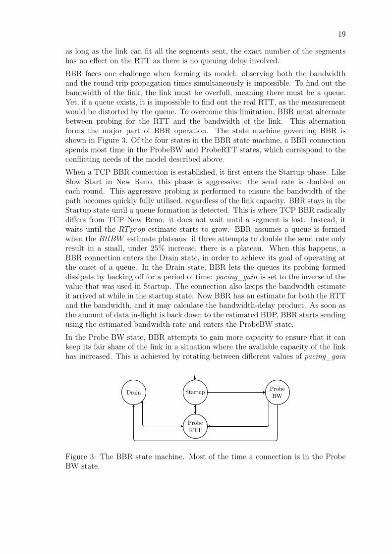
BBR faces one challenge when forming its model: observing both the bandwidthand the round trip propagation times simultaneously is impossible. To find out thebandwidth of the link, the link must be overfull, meaning there must be a queue.Yet, if a queue exists, it is impossible to find out the real RTT, as the measurementwould be distorted by the queue. To overcome this limitation, BBR must alternatebetween probing for the RTT and the bandwidth of the link. This alternationforms the major part of BBR operation. The state machine governing BBR isshown in Figure 3. Of the four states in the BBR state machine, a BBR connectionspends most time in the ProbeBW and ProbeRTT states, which correspond to theconflicting needs of the model described above.

When a TCP BBR connection is established, it first enters the Startup phase. LikeSlow Start in New Reno, this phase is aggressive: the send rate is doubled oneach round. This aggressive probing is performed to ensure the bandwidth of thepath becomes quickly fully utilised, regardless of the link capacity. BBR stays in theStartup state until a queue formation is detected. This is where TCP BBR radicallydiffers from TCP New Reno: it does not wait until a segment is lost. Instead, itwaits until the RTprop estimate starts to grow. BBR assumes a queue is formedwhen the BtlBW estimate plateaus: if three attempts to double the send rate onlyresult in a small, under 25% increase, there is a plateau. When this happens, aBBR connection enters the Drain state, in order to achieve its goal of operating atthe onset of a queue. In the Drain state, BBR lets the queues its probing formeddissipate by backing off for a period of time: pacing_gain is set to the inverse of thevalue that was used in Startup. The connection also keeps the bandwidth estimateit arrived at while in the startup state. Now BBR has an estimate for both the RTTand the bandwidth, and it may calculate the bandwidth-delay product. As soon asthe amount of data in-flight is back down to the estimated BDP, BBR starts sendingusing the estimated bandwidth rate and enters the ProbeBW state.

In the Probe BW state, BBR attempts to gain more capacity to ensure that it cankeep its fair share of the link in a situation where the available capacity of the linkhas increased. This is achieved by rotating between different values of pacing_gain

Drain Startup

Probe

RTT

Probe

BW

Figure 3: The BBR state machine. Most of the time a connection is in the ProbeBW state.

20

in a predefined manner, as shown in Figure 4, using eight phases lasting roughly theestimated round trip propagation time. If, as a result of increasing pacing_gain, thebandwidth estimate changes, BBR keeps the new estimate and the ensuing highersend rate. If it does not change, BBR backs off by lowering the send rate in a waythat allows any queues that were possibly formed to drain using a decreased valuefor pacing_gain. More precisely, the probing phase sets pacing_gain to 5/4, whilethe following phase sets it to 3/4, respectively, to clear possible queues. In the sixother phases, pacing_gain is kept at one. While the order of the phases is set, thefirst phase is randomly chosen. The randomisation lessens the likelihood of multipleBBR streams being synchronised in their probing, as well as ensures fair cooperationwith possible other algorithms using the same link. Only the phase that decreasesthe rate is excluded from being the first phase. This is natural as the decrease isonly used to dissipate possible queues. Changing the values of pacing_gain in thismanner results in a wave-like send rate pattern as depicted in Figure 5.

Whenever a TCP BBR flow has been sending continuously for the duration of anentire RTprop window, and it has not observed a RTT sample that would eitherdecrease the current RTprop value or match it for ten seconds, the Probe RTTstate is entered. Most commonly this is from the Probe BW state. In this statethe congestion window is set to four. The goal of the Probe RTT state is to ensureall concurrent BBR flows are sending with this small window simultaneously for atleast a short period of time so that any possible queue in the bottleneck is drained,and the minimum RTT can be accurately estimated. After maintaining this statefor at least 200 milliseconds and one RTT, the state is exited. If the estimates at theend of Probe RTT show that the pipe is not full, the next state is Startup, whichattempts to fill the pipe. Otherwise the next state is Probe BW.

5/4

3/4

1

1

1

1

1

1

Figure 4: When in the Probe BW state, TCP BBR alternates between eight differentstates in a circular fashion, and pacing_gain is set according to the state. Any ofthe eight states except for the one that sets pacing gain to 3/4 may be accessed first.

21

TCP BBR also differs from the other common congestion control algorithms inthe way it handles losses [JCCY19]. It assumes that a loss event signals changesin the path, warranting a more conservative approach. Further, it considers anRTO expiration to signal the loss of all unacknowledged segments, and thereforebegins the recovery by retransmitting them. It then saves the current value ofthe congestion window. If the RTO expires and there is no other data waiting tobe acknowledged, the congestion window is set to one. BBR then sends a singlesegment and continues afterwards to increase send rate as it normally would, basedon the number of successfully delivered segments, either up to the target congestionwindow, or without a boundary. On the other hand, if there is some data in flightwhen the timer expires, the congestion window is set to equal the in-flight data. BBRthen begins to packet conservation: on the first round of recovery, it sends as manysegments as it receives acknowledgements. On the following rounds, it may send upto two times that number of segments. Once an RTT has passed, conservation ends.When the loss recovery is finished, BBR restores congestion window to the value ithad before entering recovery.

0.7

0.8

0.9

1

1.1

1.2

1.3

0 5 10 15 20 25 30 35

Gain

fact

or

for

send r

ate

Phase in ProbeBW

Fluctuations in the gain factor for send rate

Figure 5: The send rate fluctuates as pacing gain values are rotated in the ProbeBW state.

3.3 CoAP Congestion Control

A single smart object might not generate a significant amount of data. However,even IoT devices may need congestion control as a large number of these smalldevices together may cause congestion, if they are using the same bottleneck linkat the same time. For example, a sensor network consisting of accelerometers maydetect the same seismic event at the same time. When all of the nodes react tothe event simultaneously, they cause a spike in traffic. This in turn may causecongestion [BGDP16].

22

The Default CoAP congestion control

CoAP needs to be usable even in extremely constrained IoT devices. These devicesmay have very little RAM, which limits, for example, the amount of state informa-tion that can be kept at a time. Consequently, CoAP lacks sophisticated congestioncontrol. The main congestion control mechanism of CoAP is to limit the numberof outstanding interactions to a particular host to one, as described in Chapter 2.2.Additionally, it employs a simple exponential back-off in case a message is deemedlost. When a new confirmable message is sent, the RTO timer is set to a randomvalue between two and three seconds. If no acknowledgement is received before thetimer expires, the timer value is doubled for the next attempt, and the message isretransmitted. By default, after four failed retransmission attempts, the messageis discarded. At most, the retransmission timeout can be 48 seconds: this is forthe fourth retransmission. A message that requires all the four retransmissions butnever receives an acknowledgement may at maximum require altogether 93 secondsof waiting for the expiration. Figure 6 shows the timing of the transmissions insuch a case. As only one message can be in flight at a time for a given connection,there are no holes to be filled and thus no duplicate acknowledgements that wouldindicate some messages did arrive while others are still missing. Thus the expira-tion of the retransmission timer is the only way for CoAP to deduce that it shouldresend a message. The CoAP specification allows implementations to change boththe maximum number of retransmissions and the number of concurrent outstandinginteractions (NSTART).

3 s6 s 12 s

45 s 93 s

4th retransmission3rd retransmission

2nd retransmission

1st retransmission

Initial transmission

Transmission discarded

0 s3 s

9 s 21 s24 s 48 s

Figure 6: CoAP transmissions for a message when the initial RTO is set to threeseconds. The lower numbers are the binary exponential back-off value while theupper numbers show the time.

CoCoA

The stateless CoAP default congestion control of is extremely straightforward andconsequently may perform poorly. The more sophisticated CoAP Simple Con-gestion Control/Advanced (CoCoA) congestion control, aims to remedy the situ-ation [BBGD18]. CoCoA has been shown to improve the throughput, the latency,and the ability to recover from bursts in many different settings and scenarios,and to perform at least as well as the Default CoAP congestion control [BGDP16,BGDP15, JDK15]. The most notable difference between CoCoA and the DefaultCoAP congestion control is that CoCoA keeps more state information, allowing it to

23

take into account the state of the network. Namely, CoCoA continuously measuresthe RTT between endpoints, attempts estimates the actual RTT of the link basedon these samples, and changes its RTO value based on the estimate. Consequently,CoCoA is able react to network events in a more flexible way than the Default CoAPcongestion control.

The RTO estimation in CoCoA is modelled after the TCP RTO estimation. How-ever, to be better adapted to constrained networks, some changes were introduced.Unlike TCP, which must use Karn’s algorithm [KP87], CoCoA does not discardambiguous RTT samples [PACS11]. That is, samples measured from segments thatwere retransmitted before receiving an acknowledgement. These samples are am-biguous because it is not clear whether the ACK was sent based on the originaltransmission or one of the later ones. The ambiguous samples are taken into ac-count in CoCoA because it is expected that in IoT networks packet loss indicateslink errors rather than congestion [BGDP16]. This is also why CoCoA employs twoRTO estimators: the strong (6) and the weak estimator (7). The strong estimator isupdated when an acknowledgement arrives before any retransmissions are required.Conversely, the weak estimator is updated when an acknowledgement for a first ora second retransmission arrives: that is, if the acknowledgement arrives before thethird retransmission has been sent. Any responses arriving after the third retrans-mission is sent are ignored. The current RTO estimate is based on the estimatorthat was last updated. In this way CoCoA can benefit from the less reliable sampleswithout placing undue weight on their importance. In case retransmissions are re-quired, it is ambiguous which transmission of a message is being acknowledged. Forthis reason, when updating the weak estimator, CoCoA calculates the RTT usingthe initial transmission time instead of any of the later transmission attempts.

RTOnew := 0.5 · Estrong + 0.5 ·RTOprevious (6)

RTOnew := 0.25 · Eweak + 0.75 ·RTOprevious (7)

Backoff logic for CoCoA differs from the Default CoAP. Both the weak and thestrong estimator are based on the algorithm for computing TCP’s retransmissiontimer [PACS11], presented in Section 3.2. However, some differences exist. First, avariable back-off (VBF) is used. In case the current RTO is less than a second, thenew RTO will be 3 ·RTO so that the retransmissions are spread out sufficiently anddo not expire too quickly, even if the initial RTO was very low. For example, if theRTO is 0.9 seconds it is multiplied by 3 as per the lower limit of the variable back-off,resulting in an RTO estimate of 2.7 seconds. If the RTO falls between one and threeseconds, the new RTO will be 2 ·RTO as in the base CoAP definition. Finally, if thecurrent RTO is higher than three seconds, the new RTO is 1.5 ·RTO. This ensuresthat retransmissions can be handled within the specified maximum time a transmitmay take, even if the initial RTO was large. Second, the initial RTO is doubled inCoCoA, and is thus two seconds unless the endpoint communicates with multipleendpoints, in which case the initial RTO is two seconds times the number of parallel

24

exchanges. Third, the constant K used in the RTO estimation as a multiplier forRTTVAR has been decreased from four to one for the weak estimator, in orderto ensure a high RTTVAR does not lead to a rapid growth of the RTO estimate.This could easily happen in a situation where an ambiguous measurement is madeafter one or two retransmits. For the strong estimate, K is kept four. Finally,the exponential back-off is not allowed to grow over 32 seconds. CoCoA dithersretransmissions between 1·RTO and 1.5·RTO as in the CoAP base definition.

RTO := 1s+ (0.5 ·RTO) (8)

Another distinct feature of CoCoA is ageing. Both small and large estimator valuesare aged if they do not receive updates. An estimator is doubled, if its value staysunder one second without updates for 16 times its current value. This is helpful inpreventing spurious RTOs. If after a long period of low, below 1 second, RTOs theconnection suddenly worsens considerably, and no new RTT measurements are madebecause of packet losses and long delays, aging ensures that the RTO estimate isquickly increased. Likewise, if the value of an estimator is higher than three secondsand it is not updated for four times its current value, the value is set according toequation 8. For example, if the RTO has reached 4.5 seconds, and is not updated for18 seconds (4·4.5 = 18), it is reduced to 3.25 seconds (1s+0.5·4.5 = 3.25). This waythe ageing mechanisms help CoCoA more quickly return to normal function aftera burst. Finally, the recommended minimum time to keep an RTO value is 255seconds, a little over 4 minutes. This is to diminish the chance that an unsuitableinitial RTO value is used when a better estimate would be available.

CoCoA and CoAP performance

CoCoA achieves better throughput than Default CoAP when congestion level is highbecause it can adapt the RTO value to the traffic level, and consequently needs fewerretransmissions. Default CoAP has been found to outperform CoCoA only underlight load. In this case CoCoA suffered from occasional spurious retransmissions ifits RTO estimate tracked the RTT too closely. Default CoAP avoids such problemsbecause of its fixed RTO range [BGDP13]. However, this observation was madeusing an older version of CoCoA. The current version includes the variable backofffactor and other changes to the RTO calculation that should prevent the problem.

In contrast, a later study found CoCoA to use too high RTO values during highcongestion. This motivated an improved version of CoCoA, CoCoA+, that aimedto limit extreme RTO values. CoCoA+ was found to be more reliable in comparisonto both Default CoAP and the CoCoA draft of the time. It better handled suddenchanges and also adapted to different levels of congestion: in 5 out 8 cases CoCoA+also achieved the lowest settling time after a burst. In the two cases where thethen-current CoCoA did settle faster than CoCoA+, the ratio of successfully sentsegments to all segments was still better for CoCoA+: it sacrificed settling speedfor reliability. [BGDP15]

25

Another study employing CoCoA+ with minor tweaks to variable values confirmedthese results [BGDK14]. The changes introduced in CoCoA+ have been incorpo-rated into the CoCoA draft after some further refinements, and so these resultsshould be applicable to current CoCoA as well.

However, CoCoA still occasionally suffers from too high RTO values, caused bythe contributions of the weak estimator [JRCK18a, BSP16, JDK15]. This mayhappen when the traffic level is high [JDK15], when the buffer size is small, or whenthe environment is bufferbloated and the connection state frequently reset so thathistorical data is not readily available [JRCK18a]. The variable backoff factor limitsextremities, which might cause further retransmissions. In such a case CoCoA hasbeen seen to have generally high RTOs and yet require notably many retransmissionscompared with Default CoAP [JRCK18a]. On the other hand, Default CoAP isalso shown to often retransmit unnecessarily under high load. This is especiallypronounced when buffer size is very large. Default CoAP resets the RTO for eachnew message, even if for the previous one the default value was found to be too low.As the link is congested, some spurious retransmissions are dropped from the routerqueue, yet consuming resources of the link, and causing delay for useful traffic.Indeed, when congestion level is high, and the buffer in the bottleneck is large,CoCoA is able to complete a transfer faster than the Default CoAP, and it likewiserequires fewer retransmits. Finally, when errors are introduced into the network,CoCoA flows complete quicker than Default CoAP flows, especially when the errorrate is high. This again is because of the adaptive RTO, which is often lower thanfor Default CoAP [JRCK18a].

Newer results confirm the efficiency of CoCoA over Default CoAP [BGDP16, JDK15,JRCK18a, JRCK18b], although under certain specific conditions Default CoAP maystill outperfom CoCoA [BSP16, JRCK18a]. CoCoA is found to have higher through-put, shorter flow completion time, and fewer retransmits than CoAP [JDK15]. Evenwhen the network is lossy, CoCoA is able to adjust the RTO correctly and avoidbogus values. In contrast, CoAP does not adapt so it cannot perform as well asCoCoA. It uses a fixed range of RTO values, cutting off values low and high thatmight be useful under certain conditions. If the RTT is actually lower than theRTO range allows, the capacity of the link is not utilised well as retransmitting isdone too conservatively. On the other hand, if RTT is equal to, or, greater thanwhat the RTO range allows, spurious retransmissions are likely. [BGDP16] If suchunnecessary retransmissions occur, they may even lead to a worse congestive state,causing further losses and thereby making transmission times ever longer as RTOvalues are backed off [JDK15]. CoCoA is able to keep sane RTO values because ofthe variable backoff factor and ageing: without them, the RTO values might growtoo large, and the overall RTO would not decay towards the default unless new up-dates were available. There would be a risk of the RTO staying artificially inflatedafter a period of inactivity [BGDP16]

26

3.4 Alternatives to CoCoA

In addition to the Default CoAP congestion control and the improved CoCoA con-gestion control, various other algorithms have been studied in the constrained set-ting. The congestion control algorithms discussed here include some specificallydesigned for use by CoAP, such as CoCoA-Fast, CoCoA-S, and CoCoA-Strong, aswell as CoAP implementations of RTO algorithms originally designed for TCP butadapted to CoAP, namely Linux RTO, and Peak-Hopper. These alternatives arecompared to CoCoA, as it has been shown to perform better than CoAP, and animproved congestion control algorithm should be able to outperform it.

Simple CoCoA variants

The key improvement of CoCoA over CoAP is the ability to react to the networkenvironment by keeping track of the measured RTT values and adjusting the RTOtimer accordingly. CoCoA attempts to leverage the information available in the formof acknowledgements arriving after retransmissions despite the ambiguous nature ofsuch RTT values. Consequently, the study of CoCoA has focused on tuning therelated parameters and mechanisms.

CoCoA+ featured improvements that proved to be useful, and so were incorporatedinto the current CoCoA specification after some modifications. These include re-ducing the value of K to 1, replacing the original binary exponential backoff witha variable backoff factor, and ageing for values that are high as before CoCoA onlyaged low RTO values [BGDP15].

CoCoA-Strong does not react to a single loss: on subsequent losses and otherwiseit behaves exactly as CoCoA. The reasoning behind the change is the expectationthat losses are due to link errors rather than congestion. While this behaviour maycause worse congestion in case the first loss was indeed due to congestion, it mayalso help in sending more promptly in the face of link errors. [BSP16]

CoCoA-Fast also behaves as CoCoA but the values of the variable backoff factorsand the backoff threshold, as well as both the initial and the maximum RTO, arereduced to make its behaviour more aggressive: CoCoA RTO values have beenshown to reach values too high above the actual RTT. This is especially pronouncedin an environment where wireless loss is frequent: CoCoA is not able to distinguishbetween congestion and link errors. CoCoA-Fast is shown to have more realisticRTO values yet it is claimed to still be too conservative. [BSP16]

CoCoA-S [BGDP16, BGDP13] only employs the strong estimate, but is otherwisethe same as CoCoA. It requires less state information, making it a lightweight al-ternative to the full CoCoA [BGDP13]. The lack of the weak estimator preventsCoCoA-S from achieving accurate RTT estimates, especially when the link faces highlevels of traffic [BGDP13], and it tends to have lower RTO values than baseline Co-CoA [BGDP16]. Consequently CoCoA outperforms it. CoCoA-S does have shorteridle periods after losses [BGDP13], but at the same time it is too aggressive in face of

27

bursts, and the lower RTOs increase the likelihood of spurious retransmissions whenthe RTT estimate is very close to the actual RTT [BGDP16]. This makes CoCoA-Sless efficient in reducing the number of packets in buffers, leading to more droppedpackets, that is, less efficient usage of the available bandwidth [BGDP13]. Despitethese shortcomings, CoCoA-S outperforms Default CoAP as it can adapt the RTOto the conditions of the network [BGDP13]. Variable back-off factor and the ageingmechanism help it to avoid too high RTO values [BGDP16]. CoCoA-S is especiallysuitable for low-RTT connections over a link that suffers few losses [BGDP16].

Alternative RTO algorithms

Some alternative RTO algorithms have also been studied in the constrained set-ting [BGDP16, JDK15, BKG13]. Here are discussed two well-known TCP RTOalgorithms, Peak-Hopper [EL04] and Linux RTO [SK02]. Both identify problemswith the RFC 6298 [PACS11] RTO algorithm, preceded by RFC 2988 [PA00], andaim to remedy those.

Linux RTO identifies two problems. The first one is too high RTO caused by suddendrops in RTT that make RTTVAR grow, while the second one is spurious retrans-missions caused by the RTO tracking the RTT too closely. Linux RTO introducestwo changes. First, the effect that the variance term has on the SRTT is loweredin cases where the RTT sample measured is notably lower than the smoothed av-erage. RTO is not increased if the most recent RTT sample shows that the RTTis decreasing below the RTT values that were available before. This enables it toavoid RTO peaks when it deems the link conditions to be improving. It does decaythe RTO value if the following RTT samples stay low. Second, Linux RTO uses aspecial mean deviance variable to reduce the effect of RTTVAR. It may be updatedmore often than RTTVAR, which may only be reduced once in an RTT. If thisvariable produces a higher estimate, RTTVAR is increased immediately, so that ineffect RTTVAR is a maximum of this variable and the last RTT. [SK02]

Peak-Hopper identifies more problems, the key ones being slow response to RTTpeaks, conservative reaction to sudden low RTT, too short history of RTT sam-ples, and too low minimum RTO. Peak-Hopper was designed for situations whereother means of detecting loss are unsuitable, for example, when there are too fewacknowledgements in flight to enable the use of a more sophisticated loss recoverymechanism. The key idea in Peak-Hopper is that the reaction to a decreasing RTTestimate should be cautious and that, on the other hand, a growing RTT estimatewarrants an aggressive reaction. Additionally, the RTO should depend on the RTTvariance. Like CoCoA, Peak-Hopper employs two RTO algorithms: the short-termhistory and the long-term history. The first one takes into account the currentsituation and recent events. It responds to a growing RTT. The latter is used toslowly decay the current RTO. Peak-Hopper always chooses the maximum of thesetwo RTO estimates. In case the short-term history captures an increase in RTT,the long-term history is reset, and the RTO calculation is based on the short-termestimate. [EL04]

28

CoCoA might be more suitable for IoT settings than the protocols that have beendesigned for more general use cases [BGDP16]. Compared to two other RTT-basedalgorithms, namely Linux RTO and Peak-Hopper, CoCoA behaves in a stable way:all flows complete in roughly the same time compared to Peak-Hopper, for whichsome flows take notably long time to finish [JDK15].

The two algorithms perform similarly in constrained settings. Both are clearly animprovement over the Default CoAP fixed range RTO, but comparing to CoCoA,the results are mixed. As neither takes into account ambiguous samples, they maysometimes have low RTO values and resend too aggressively. Linux RTO [BGDP16]or both [JDK15] have been noted to use very low RTO values. Too aggressive RTOvalues lead to spurious retransmissions, and both have been shown to need more re-transmissions than CoCoA [BGDP16, JDK15]. Consequently, both may have worseaverage throughput than CoCoA [BGDP16], and during very high congestion, LinuxRTO and Peak-Hopper clients may take notably long to finish their transactions,which is partly explained by the number of retransmissions [JDK15]. As the retrans-missions have exponential backoffs, the delays caused may be very long [JDK15].

Additionally, both have also been shown to maintain these large backed off RTOvalues, and to reuse them for new transactions when multiple retransmissions havetaken place. If packets are frequently lost, idle periods due to high RTO occuroften [BGDP16]. For Peak-Hopper specifically, the way it quickly reacts to signs ofincreasing traffic may lead to high RTO values that are kept too long because theRTO does not decay quickly enough. In case the RTT naturally fluctuates, whichmay be typical in an IoT scenario, the quick increase in RTO may be unwarranted:when packets are lost, an unnecessarily high RTO value is used because the RTOis not lowered quickly enough, delaying retransmissions [BGDP16]. Finally, thenature of Peak-Hopper is visible in burst recovery, which may be time-consuming:RTT peaks cause the RTO value to grow quickly but new samples showing a lowerRTT have no such effect: instead the RTO decays slowly [BGDP16].

Due to these phenomena, Linux RTO and Peak-Hopper are not able to outper-form CoCoA, and in general do not adapt well to IoT communication patterns andenvironments [BGDP16]. The algorithms might benefit from including weak sam-ples [BGDP16] but including only unambiguous samples has the benefit of avoidingneedlessly high RTO values [JDK15]. For example, if there are many retransmis-sions, the weak estimator of CoCoA makes the RTO grow very high. As these twoalgorithms ignore ambiguous samples, they are able to act more efficiently. Thus,when congestion is high, they have also been shown to outperform CoCoA. In suchhigh congestion scenarios some Linux RTO and Peak-Hopper clients were very slowto finish transactions, yet still the median completion times these algorithms at-tained were low compared to CoCoa. It should be noted that in this study themaximum RTO value for Peak-Hopper and Linux RTO was 60 while for CoCoA itwas the default 32 seconds, which may in part explain these long tails. Additionally,they also were able to successfully finish a CON-ACK pair transaction on the firstattempt more often [JDK15].

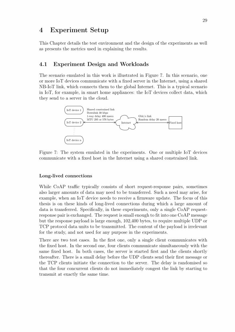
29

4 Experiment Setup

This Chapter details the test environment and the design of the experiments as wellas presents the metrics used in explaining the results.

4.1 Experiment Design and Workloads

The scenario emulated in this work is illustrated in Figure 7. In this scenario, oneor more IoT devices communicate with a fixed server in the Internet, using a sharedNB-IoT link, which connects them to the global Internet. This is a typical scenarioin IoT, for example, in smart home appliances: the IoT devices collect data, whichthey send to a server in the cloud.

IoT device n

IoT device 1

IoT device 2

Shared constrained link

Downlink 30 kbps

1-way delay 400 msecs

MTU 295 or 576 bytes

Internet Fixed host

Gbit/s link

Random delay 20 msecs

Figure 7: The system emulated in the experiments. One or multiple IoT devicescommunicate with a fixed host in the Internet using a shared constrained link.

Long-lived connections

While CoAP traffic typically consists of short request-response pairs, sometimesalso larger amounts of data may need to be transferred. Such a need may arise, forexample, when an IoT device needs to receive a firmware update. The focus of thisthesis is on these kinds of long-lived connections during which a large amount ofdata is transferred. Specifically, in these experiments, only a single CoAP request-response pair is exchanged. The request is small enough to fit into one CoAPmessagebut the response payload is large enough, 102,400 bytes, to require multiple UDP orTCP protocol data units to be transmitted. The content of the payload is irrelevantfor the study, and not used for any purpose in the experiments.

There are two test cases. In the first one, only a single client communicates withthe fixed host. In the second one, four clients communicate simultaneously with thesame fixed host. In both cases, the server is started first and the clients shortlythereafter. There is a small delay before the UDP clients send their first message orthe TCP clients initiate the connection to the server. The delay is randomised sothat the four concurrent clients do not immediately congest the link by starting totransmit at exactly the same time.

30

UDP transfer details

Figure 8 illustrates the progression of a UDP flow. In this case, Block-Wise Transferpresented in Section 2.2 needs to be used. First, the server is started. Then, theclient sends a request to the server—the request does not include Block-Wise options.The server then responds with the first block of the transfer, including in the messagethe necessary Block-Wise options. When the client in this way has received the firstblock, it requests the subsequent block. Again, the server responds and the clientrequests a new block. This is repeated until the client has received the block withthe More bit unset, indicating that this block is the last one. The block size in thissetting is 256 bytes, and the client accepts this size without further negotiation.

CON 1, GET, /hello

ACK 1, 2.05 Content, 2:0/1/4 (256)

CON 2, GET, /hello, 1:1/0/4 (256)

ACK 2, 2.05 Content, 2:1/1/4

CON 3, GET, /hello, 2:2/0/4

ACK 400, 2.05 Content, 2:400/0/

4

Client Fixed host

Figure 8: Transferring a large payload using block-wise transfer with the Blockoption 2. A client requests a resource which is too large to fit into a single CoAPmessage. The server indicates it will use block-wise transfer such that the block sizeis set to 4, that is, 256-bit blocks are transferred. The client agrees with the sizeand requests the block it wishes to receive next. The More bit is set in all but thelast block the server sends.

TCP transfer details

A CoAP over TCP flow proceeds as follows. First, the server is started. It doesnot wait for the client to send its CSM before sending its own. Before initiating aconnection to the fixed host, the client waits for a random period of time. After theinitiation, the client sends its CSM, immediately followed by its request. Finally,

31

when the server receives the request of the client, it starts sending the large reply.When the traffic is carried over TCP, Block-Wise Transfer is not used. Instead,the large reply is a single CoAP message, carried in multiple TCP segments, out ofwhich only the first one includes the CoAP headers.

Like the payload, the CSM messages are not significant, and are discarded. They areonly included to conform with the specification and to provide additional burden onthe network. As the CoAP over TCP headers include the message length, the clientknows when the transfer is complete. The MTU for the link is 296 bytes, leaving256 bytes for payload after the IP and TCP headers. Thus the entire transfer takes401 TCP segments, which is roughly the same as in the UDP setup.

Short-lived connections

In addition to the results presented in this thesis, also short-lived connectionswere evaluated in the environment described in this Chapter [JPR+18, JRCK18a,JRCK18b]. In the workload for short-lived connections, the clients exchange short60-byte CoAP messages with the same fixed server. Two types of clients were em-ployed: continuous and random. Continuous clients keep exchanging messages untilaltogether 50 have been exchanged. Random clients exchange altogether 50 mes-sages, in random-sized batches of 1 to 10 messages. The connection state is resetafter each batch, meaning that all congestion control related variables are set to theirdefault values, and that a TCP client will initiate a new connection. The numberof simultaneous clients is varied between 1 and 400.

4.2 Network Setup and Implementation Details

The network setup emulates an NB-IoT-type link as detailed in Table 4. Down-stream, the link has a data rate of 30 kbps and a one-way delay of 400 milliseconds.Upstream, the link has a data rate of 60 kbps and a one-way delay of 200 millisec-onds. The maximum transfer unit (MTU) for the link is 296 bytes. To emulatea variable delay for the rest of the path between the last-hop router and the fixedhost, a 10-20 millisecond delay with random variation is used.

Retransmissions and other congestion control-related events are triggered accordingto the mechanisms of the congestion control mechanism employed in each particular

Downlink UplinkNB-IoT data rate 30 kbps 60 kbps1-way delay 400 msecs 200 msecsBottleneck buffer size 2500 B, 14100 B, 28200 B, or 14100 BMTU 296 B

Table 4: Network parameters of NB-IoT and the bottleneck buffer size used in theexperiments.

32

test case. For CoAP over UDP both the CoAP default congestion control and themore advanced CoCoA congestion control are used. For CoAP over TCP trafficboth TCP New Reno and TCP BBR are used.

In the experiments, four different sizes of buffers are used for the bottleneck router.The smallest buffer is only 2500 bytes, which is approximately the bandwidth-delayproduct (BDP) of the link. In contrast, the largest buffer size is 1,410,000 bytes,which can easily fit all of the payload. This buffer size is also referred to as theinfinite buffer. The middle-sized buffers are 14,100 bytes and 28,200 bytes. Thethree largest buffers cause bufferbloat.

The likelihood of bit-errors in the link is also varied. In the base case, the networkis entirely free of errors, and all packet loss is due to congestion. To study how thecongestion controls differ in their ability to recover from packet loss, three differenterror profiles are used.

These three states are low, medium, and high, detailed in Table 5. In the case ofthe low error rate, the packet error rate is a constant 2%. In the other two casesthe error rate varies, resulting in an average of 10% and 18% for the medium andthe high error profile, respectively. The errors are introduced using a Markov modelthat alternates in suitably short intervals between two states: the error-burst and thelow-error state. Notably, in this test setup, it is possible for multiple retransmissionsof the same packet to be lost, making recovery particularly challenging.

Low constant 2%Medium 10% in average alternating between 0% and 50%High 18% in average alternating between 2% and 80 %

Table 5: Packet error profiles and their states.

Network emulation details

Figure 9 i) shows the test environment, which consists of four physical Linux hostsconnected by high-speed physical links. The client software emulating the IoT de-vices is deployed in host 1, while the fixed server software is deployed in host 4. Hosts2 and 3 are used to emulate the network using two instances of the netem networkemulator. The first instance emulates the upstream and the second instance thedownstream. In this way, a message passing through the emulated network alwayspasses through two instances of emulators in total. The first emulator emulates thebit rate of the bottleneck link and the buffer of the bottleneck router. The secondemulator emulates the propagation delay and the packet loss occurring in the wire-less link, in the event there are any. The second emulator has a very large bufferto ensure no packets are dropped due to congestion. This setup ensures the routerbuffer size is correctly emulated, and that the capacity of the link is consumed as itshould, even when a packet is dropped due to an emulated wireless error.

33

Figure 9 ii) explains the role of each host on the path of a packet that travels fromthe fixed host to an IoT device.

The server and client programs are implemented in C99 using the libcoap CoAPlibrary for C [libcoap]. The libcoap library was extended to implement support forCoAP over TCP.

Host 3

Fixed HostInternet

Downstream netememulates:- bitrate- buffer of thebottleneck router

Upstream netememulates:- propagation delay- packet losses

Host 4

Fixed Host

Host 2

Upstream netememulates:- bitrate- buffer of thebottleneck router

Downstream netememulates:- propagation delay- packet losses

IoT device 1

IoT device 2

IoT device n

Host 1

IoT device

Wirelesslink

i)

ii)

Propagation delay

Packet loss rate:average 0-30%

Low bitrate link:downlink30 kbps

Last hop routerBuffer size:bandwidth-delay product orbufferbloat

Figure 9: The test setup. i) shows the role of each real host. ii) the role of all thehosts in the emulation of a downlink connection.

Implementation details

In the experiments, Default CoAP is implemented as per RFC7252 [SHB14], CoCoAas per the draft [BBGD18] and CoAP over TCP as per the draft [BLT+17]. TheLinux TCP implementation is altered in the following way: Cubic [RXH+18, HRX08]congestion control, Selective Acknowledgements [MMFR96], and Forward RTO-Recovery [SKYH09] are disabled in order to use TCP New Reno congestion con-trol [HFGN12]. Further, Control Block Interdependence [Tou97] is disabled and theTCP Timestamp [BBJS14] option is not used. This configuration is to make theLinux kernel TCP implementation more akin to the standardised TCP and moresuitable for constrained devices. Tail Loss Probe [DCCM13], RACK [CCD18], andTCP Fast Open [CCRJ14] are disabled as well. The Initial Window [AFP02] valuein the experiments is set to four segments. Finally, the Linux TCP implementationis configured to use an initial RTO of two seconds, and to send delayed acknowl-edgements with timer set to a constant 200 milliseconds.

Some changes are introduced to the CoAP congestion control, too. MAX_RETRANSMITis set to 20, EXCHANGE_LIFETIME and MAX_TRANSMIT_WAIT are adjusted according

34

to the CoAP specification [SHB14], and, to avoid premature failures, SYN andSYN/ACK retries in the Linux TCP are increased to 40 and 41, respectively. Thisis to avoid too early termination in the case the network is highly congested.

The default upper bound for RTO timeout in the Linux TCP implementation is120 seconds and is left as-is. CoCoA [BBGD18] truncates the binary exponentialbackoff at 32 seconds. For Default CoAP, 60 seconds is used, as no maximum valueis defined and very long retransmission timeouts are undesirable.

4.3 Metrics

The primary metric is the Flow Completion Time (FCT). This is the time elapsedfrom when the client sends a request until the client receives the last protocol dataunit of the requested object. In the case of TCP, this metric does not include theconnection initialisation which is measured separately. For the four client case, theFCT is calculated separately for single flows within a test run, and not the time ittook for the whole test run to be finished.

Other, secondary, metrics are used in explaining the phenomena contributing to theachieved FCT. These secondary metrics include:

1. Packet loss rate

2. Number of RTO timeouts

3. Frequency of transmissions: the number of (re)transmissions needed for thesuccessful exchange of a request-response pair

4. Number of protocol data units sent in total

These metrics are available for both connection ends but for the most part the fixed-end results are discussed as the client only sends a single, short request. All the testsare replicated at least 20 times. The results of all the replications are included incalculating the metrics. The metrics are derived from tcpdump traces collected fromall the interfaces of all the nodes in the test environment.

For TCP, the secondary metrics relating to RTOs are calculated from the pre- andpost-run metrics attained from the Linux kernel, and as such they may have slightinaccuracies that do not affect the general observations that can be made from them.

The payload in the Firmware Update Traffic test case is 102,408 bytes which consistsof the actual payload of 102,400 bytes and the 8-byte CoAP over TCP headers.With a MSS of 296 bytes this results in 401 segments since the minimal TCP andIP headers take 40 bytes of each segment. This means that for one Firmware Updatetransfer 16,040 bytes of headers are transferred altogether. This does not includethe handshake, the initial request, or the CSM message headers. In the ideal case,the TCP-based transfers should take 32.2 seconds per client.

35

5 Related Results

This Chapter discusses recent research in CoAP congestion control and CoAP overTCP performance. All results presented here were obtained in the environmentdescribed in the previous Chapter, using the short-lived connection workload. ThisChapter begins with an explanation of how baseline CoAP and CoCoA may lead tocongestive collapse, and how to prevent it. This is followed by an introduction toan improved congestion control for CoAP over UDP. Last presented are the resultsof our evaluation of CoAP over TCP performance for short-lived connections.

5.1 CoAP over UDP

Congestion collapse risk in CoAP and CoCoA

CoCoA clearly improves the ability to react to congestion when using CoAP. How-ever, recently both CoAP and CoCoA have been shown to be vulnerable to conges-tion collapse in a highly congested, bufferbloated environment [JRCK18b]. As thebuffer sizes grow and the amount of traffic in the link is high, the queuing delaysfor CoAP grow in an unsustainable way. The buffer is filled with unneeded re-transmissions, wasting the link capacity. CoCoA behaves better than Default CoAPcongestion control, but under certain traffic patterns, namely, when the connec-tions are short-lived, it shows the same symptoms of congestion collapse as DefaultCoAP. In this case, with a large number of concurrent senders, the collapse is evenworse for CoCoA. Because of its variable back-off factor, CoCoA ends up using lowerRTO values than Default CoAP. However, both congestion controls may be modi-fied so that they are no longer prone to cause congestion collapse [JRCK18b]. Thesecongestion-safe variants are called Full Backoff 1 and Full Backoff 2.

Full Backoff 1 for CoAP changes the baseline CoAP behaviour so that if a CoAPsender needs to retransmit a message, it will retain the backed off RTO value untilit is able to exchange a CON-ACK pair without retransmits. If the backed offtimer expires during the next exchange, the regular binary exponential backoff isapplied. If a successful exchange is achieved, the initial RTO is returned to. Whilethis change was shown to prevent a congestion collapse, the resulting behaviour isstill quite aggressive in cases where latency is high, so an additional variant, FullBackoff 2 was created. Using Full Backoff 2, if a successful exchange is achieved,the backed off RTO is halved after each successful exchange until the RTO is backat the initial value.

Full Backoff 1 for CoCoA retains the backed off RTO. However, this does not takeinto account the weak RTO estimator updates: updating the weak estimator maylead to a notable increase in the RTO. In order to address that concern, Full Back-off 2 picks the maximum of the current RTO and the newly updated RTO. Thebacked off RTO is then based on the maximum, and used for the following exchange.

36

For CoAP, Full Backoff 1 is clearly more safe than the regular Default CoAP con-gestion control while Full Backoff version 2 has an even larger impact on number ofunneeded retransmissions. This effect is also visible when the random clients wereevaluated. Random clients are more challenging, since the senders reset their stateconstantly, and consequently cannot benefit from historical data.

Full Backoff versions for CoCoA also manage to completely avoid the congestioncollapse that would otherwise be a risk with the random-type workload and thelargest buffer. As was the case with Default CoAP, the more conservative version2 is even more effective than the version 1. Although CoCoA is not susceptible tocongestion collapse when the traffic is continuous, or when the traffic is random andthe buffers are small and the number of concurrent clients is low, it still benefitsform the Full Backoff variants. In all random traffic scenarios the FCT is improved,and in the continuous traffic scenarios Full Backoff variants do at least as well orslightly better than baseline CoCoA.

All the Full Backoff variants have a clear effect on the median flow completion timeon the large buffers—especially when the largest buffer is used and the traffic is at itshighest. The more conservative behaviour is well reflected in the median number ofspurious retransmissions: at most, there is an 88% improvement compared with thecongestion-unsafe version. Full Backoff 2 variants remedy the problems that wereuncovered, and clients employing these congestion controls complete much fasterthan the original versions. They are also shown to be slightly more efficient thanthe 1 variants. Especially the number of spurious retransmissions is lowered.

FASOR

The congestion safe versions of CoCoA proved to be more efficient than the faultyCoCoA under most circumstances [JRCK18b]. However, the usefulness of CoCoAand similar approaches is diminished if the clients send data infrequently [JDK15].To achieve a more versatile congestion control, an entirely different approach mightbe needed. One way to achieve more granular control over suitable RTO values andbetter ability take into account historical data is to use a state machine to makedecisions about suitable RTO values and back off logic. Two such models haverecently been introduced [JRCK18a, BSP16]. Here presented is FASOR, Fast-SlowRetransmission Timeout and Congestion Control Algorithm for CoAP [JKRC18].FASOR introduces a new backoff logic and algorithm for RTO computation forcongestion control. FASOR aims to distinguish between bit errors and congestion,and to react efficiently to both. FASOR achieves this by employing two distinctRTO algorithms and a state machine that dictates the way the RTO is backed off.

Fast RTO is computed as defined in RFC 6298 [PACS11] with the exception of notsetting a lower bound: as RTO is the only way CoAP can detect losses, it shouldbe able to reflect RTT values below 1 second. Fast RTO is only calculated usingunambiguous samples, tracking closely the actual RTT. If link errors are assumed,Fast RTO is used to ensure a quick retransmit.

37

Slow RTO, on the other hand, is calculated beginning from the very first transmissionuntil the first acknowledgement, regardless of whether and how many retransmissionshave occurred. It always includes the worst-case RTT, making it very conservative.An RTO higher than the RTT lets the link drain of duplicate copies, and in this waySlow RTO ensures unambiguous samples for FASOR even in the presence of heavybufferbloat or congestion. Slow RTO is sparingly used because it may lead to longdelays.

There are three states in FASOR: Fast, Slow-Fast, and Fast-Slow-Fast. A connectionalways starts in the Fast state, and upon unambiguous samples, returns to that state,regardless of the state it was in. Upon ambiguous samples, the connection movesfrom the Fast state to the Fast-Slow-Fast, and finally to Slow-Fast, where it willstay until an unambiguous measurement is made. Ambiguous samples also triggerthe update of the Slow RTO.

The current state dictates how the connection backs off. In the Fast state, RTO iscalculated using only the Fast RTO with a binary exponential backoff. However, forthe two other states, a more complicated series of backoff logic is used first, beforereturning to the binary exponential backoff. In Fast-Slow-Fast, the RTO sequenceis: FastRTO , max (SlowRTO , 2 ·FastRTO), FastRTO ·21, . . . , 2i ·FastRTO . In Slow-Fast the RTO sequence is SlowRTO , FastRTO , FastRTO · 21, . . . , 2i · FastRTO .In the Fast-Slow-Fast state the first Fast RTO acts as a kind of a probe to see ifthe loss only reflected an intermittent error: if a second retransmit is needed, this isunlikely, and so Slow RTO is employed to drain the link. In the Slow-Fast state thepresence of congestion is already deemed likely and so Slow RTO is the first RTO.

FASOR may also be used with the token field carrying a counter that denotes whichretransmission the current message is. It makes all samples unambiguous withoutrequiring any changes to the server. FASOR also supports including retransmissioncount in the headers.

Both FASOR and FASOR with token were evaluated against the Default CoAPcongestion control, baseline CoCoA, and CoCoA Full Backoff 1, the congestion-safeCoCoA variant. FASOR performs well in all the error-free scenarios, even when the

Fast Fast-Slow-Fast Slow-Fast

Unambiguoussample

AmbiguoussampleUnambiguoussample

Unambiguoussample

AmbiguoussampleAmbiguoussample

Figure 10: The FASOR state machine.

38

number of concurrent clients is high. When the buffer size is high as well, CoCoAneeds to retransmit often. However, for both FASOR and FASOR with token, thenumber of retransmissions is negligible. The average RTT is similar regardless ofthe algorithm used, except when the client type is random and the bufferbloatedbuffer size is used. In this scenario, both the Default CoAP congestion control andCoCoA have notably high RTT values compared to either of the FASOR variants.The difference to the safe CoCoA is smaller.

Both the token and the token-free FASOR versions perform better when the trafficis continuous compared to the random traffic scenario. The random traffic type ischallenging for any congestion control mechanism, since the controlling variables arereset often. Further, typically the actual RTT is higher than the initial RTO, whichcauses at least some spurious retransmissions that waste bandwidth. Despite this,both FASOR versions manage to quickly find out a realistic RTO. This is due tothe Slow RTO, which backs of sufficiently so that an unambiguous sample may beobtained. Especially the token-employing version of FASOR fares well since it isable to achieve a realistic RTT estimate even when it needs to retransmit.

When the likelihood of errors is low and the number of clients is small enoughto not cause congestion, the differences between the congestion controls are againnon-existent. However, when the error rate is high, FASOR clearly outperformsboth the safe CoCoA and the Default CoAP. The FASOR versions also performsomewhat better than CoCoA. There is not much difference between the token andthe regular versions of FASOR. However, the median RTO is lower for the tokenversion. When the error rate grows high, it is especially crucial to estimate the RTTright. Using the token helps with this: RTO can go back to a low level faster whenthe token is employed. Indeed, when the error rate is high, the token version employsclearly lower RTOs than the non-token version. Finally, even though the randomworkflows are especially demanding, FASOR is able to perform well, outperformingboth unsafe CoCoA and the Default CoAP congestion control, despite them havingunfair advantage due to their aggressive RTO calculation.

These results indicate that FASOR and FASOR with token perform notably betterthan Default CoAP and better than CoCoA. While FASOR with token does notconsistently outperform the regular version, it proves very useful with the random-type clients, especially when the error rate is high.

5.2 CoAP over TCP for Short-Lived Connections

In addition to the results presented in this thesis, CoAP over TCP was also evaluatedfor short-lived connections in the environment detailed in the previous chapter.These results are presented here shortly. More detailed discussion of these results isavailable in our conference article [JPR+18] as well as a master’s thesis [Rai19].

In the baseline scenario where there are no errors and the number of clients is only50, the difference between TCP and UDP is insignificant. Continuous CoAP overTCP clients take approximately 200 milliseconds longer to complete than Default

39

CoAP or CoCoA clients. This is naturally due to the TCP headers. The differenceis more pronounced with the random clients, since they reset their state regularly.

As the number of the clients is increased to 50, the median FCT grows more for CoAPover TCP than it does for its UDP counterparts. However, in this setting, CoAPover TCP clients still only require roughly 5% more time than the UDP counterparts.Increasing the number of clients also causes an increase in the queuing delay. Asmore messages are introduced in the router, the perceived RTT grows. As theheaders are larger, the effect of queuing delay is also more notable, especially usingthe infinite buffer, which can hold all segments. Median FCT for the continuous TCPclients using the largest buffer is roughly 11% higher than for its UDP counterparts.When random clients are used, retransmissions are sometimes needed to completethe 3-way handshake.

As the number of clients is increased to 100, the FCT values are substantially largerbecause of the increased packet loss when using the smaller buffers and the increasedqueuing delay when using the larger buffers. With this level of congestion the ben-efits of CoAP over TCP become visible: especially when using the infinite buffer.CoAP over TCP performs clearly better than either UDP counterpart. This is be-cause it is able to better react to congestion. Karn’s algorithm makes TCP keep thebacked off RTO value until a new data segment that did not require retransmissionsis acknowledged. As a result, CoAP over TCP requires fewer retransmissions thanits UDP counterparts. On the smallest buffer, on the other hand, the CoAP overTCP FCT varies somewhat: some clients back off and consequently finish slow whileothers do not need the backing off and so finish quickly. The slowest clients finishnotably slower than the slowest clients using either CoCoA or Default CoAP. Still,even in this setup, the median value is lowest for CoAP over TCP. With this numberof clients, random clients employing Default CoAP and CoCoA perform similarlyto the continuous ones when the smallest buffer is used. CoAP over TCP, on theother hand, again is slowed down because of the overhead of the three-way hand-shake, especially if SYN and ACK segments are lost. With the largest buffer size,FCT increases for both CoCoA and CoAP over TCP compared with the continuousresults. This is due to the fact that new connections employ the initial RTO, whichis often too small in face of the now-long queuing delay, which then causes spuriousretransmits.

The flow completion times for 200 and 400 simultaneous clients are shown in Fig-ure 11. Here the link is highly congested and the difference between Default CoAPand the more advanced congestion controls grows large. On the smallest bufferCoAP over TCP clearly outperforms both Default CoAP and CoCoA with CoCoAperforming the worst. On the larger buffers, CoAP over TCP and CoCoA clearlyoutperform Default CoAP, achieving roughly similar results so that when the num-ber of simultaneous clients is 200, CoCoA achieves lower flow completion times butwhen the number of clients grows to 400, the situation is reversed. Both CoCoAand TCP measure RTT and so they are able to adjust RTO in accordance with thetraffic level. Their RTO values converge towards the actual RTT leading to a lownumber of spurious retransmissions. The advantage CoCoA has over CoAP over

40

TCP is mostly explained by the larger header overhead of TCP. Despite this, whenthe number of simultaneous clients is increased to 400, CoAP over TCP achieveslower median flow completion times. With the larger buffers the difference is notgreat but with the smallest buffer, the TCP clients complete roughly 21% fasterthan CoCoA clients.

0

200

400

600

800

1000

2500B 28200B Infinite

Flo

w c

om

ple

tion t

ime

(sec

s)

Default CoAP CoCoA CoAPoverTCP

0

500

1000

1500

2000

2500

3000

2500B 28200B Infinite

Flo

w c

om

ple

tion t

ime

(sec

s)

Default CoAP CoCoA CoAPoverTCP

Figure 11: Left to right, flow completion times for 200 and 400 simultaneous con-tinuous clients in the error-free setup [JPR+18].

The flow completion times for 10 simultaneous clients using the different error pro-files are shown in Figure 12. Similar phenomena as could be seen with the error-freenetwork is also seen in the figure. When the continuous workload is used, CoAPover TCP is able to handle high levels of congestion and random errors very well.When the error level is medium, the median FCT of Default CoAP is roughly 38 %higher than the median FCT of CoAP over TCP. Likewise, the median FCT of Co-CoA is roughly 12 % higher than the median FCT of CoAP over TCP. When theerror level is high, the differences are 35 % and 13 %, respectively, to the favourof CoAP over TCP. TCP uses a more accurate RTO calculation algorithm thanDefault CoAP or CoCoA, resulting in RTO values closer to the actual RTT thanwhat the UDP counterparts can achieve. CoCoA employs an additional weight of0.5 when it uses the strong samples in the RTO calculation: this makes it slow toreach a more realistic RTO value. It also uses the weak samples, so RTO valuesmay grow unnecessarily high. When the error rate is high, TCP results show highvariability. Even though the median FCT for continuous clients is clearly lowest forCoAP over TCP, some clients take almost as long as the slowest clients employingDefault CoAP, and longer than the slowest clients employing CoCoA. This is be-

41

cause of Karn’s algorithm, which makes recovery from random losses slow comparedwith CoCoA and Default CoAP. Thus, when consecutive segments are lost due torandom errors, CoAP over TCP waits slightly longer than the UDP variants beforeresending a segment. However, in the face of congestion, this strategy proves effi-cient, highlighting the need to react differently to losses caused by congestion andintermittent network errors.

0

50

100

150

200

250

300

350

error-free med 0/50% high 2/80%

Flo

w c

om

ple

tion t

ime

(sec

s)

Default CoAP/continuousCoCoA/continuousCoAPoverTCP/continuousDefault CoAP/randomCoCoA/randomCoAPoverTCP/random

Figure 12: Flow completion times for 10 simultaneous clients, both continu-ous and random, in the error-free and error-prone setups using the 2,500 bytebuffer [JPR+18].

Figure 13 shows the flow completion times for 200 and 400 simultaneous randomclients in the error-free setup. The random clients should prove the most problematicfor CoAP over TCP as these clients have very limited historical data available tothem and since the three-way handshake adds an overhead of at least one RTTper each random client. Indeed, as expected, in most cases CoCoA achieves clearlylower flow completion times than CoAP over TCP. Even Default CoAP performsbetter than CoAP over TCP when the two smallest buffers are used, regardless ofthe number of clients. Interestingly, however, when the number of clients is 400,the network is free of errors and the largest buffer is used, CoAP over TCP veryclearly outperforms CoCoA and Default CoAP. CoCoA is twice as slow as CoAPover TCP to complete in this setting, while Default CoAP is 134 % slower thanCoAP over TCP. As the clients are random, CoCoA is not able to adjust the RTOvalue in a timely manner. Further, queuing delay is high due to the bufferbloatedenvironment, making RTT very high. CoCoA uses RTO values similar to Default

42

CoAP, causing it to resend more aggressively than Default CoAP as it uses thevariable backoff factor of 1.5 with high RTO values instead of the higher value oftwo that Default CoAP uses. Consequently, for each message, CoCoA may need upto six retransmits. CoAP over TCP on the other hand only suffers from few spuriousretransmits, even though the handshake and the CSM message occasionally need tobe retransmitted. The number of retransmissions CoAP over TCP needs is notablylower, explaining the great performance difference.

On the other hand, in the error-prone environment, the situation with random clientsis different. This is illustrated in Figure 12, showing the flow completion times for10 simultaneous clients. Unlike in the case of continuous clients under the error-prone network, where CoAP over TCP achieved notably lower median FCT thanthe UDP counterparts, now that random clients are used, CoAP over TCP performsthe worst, especially if the likelihood of errors is high. The three-way handshakeand the CSM messages proved problematic even in the error-free setup, and lossescaused by errors further amplify the problem. With random clients, the differencebetween TCP and UDP grows smaller as the error rate increases. When the link iserror-free, the median FCT for CoAP over TCP is roughly 43% higher than it is foreither CoCoA or Default CoAP. When the error-rate is high, the median FCT forCoAP over TCP is only roughly 37% higher than for CoCoA.

0

200

400

600

800

1000

2500B 28200B Infinite

Flo

w c

om

ple

tion t

ime

(sec

s)

Default CoAP CoCoACoAPoverTCP

0

500

1000

1500

2000

2500

3000

2500B 28200B Infinite

Flo

w c

om

ple

tion t

ime

(sec

s)

Default CoAP CoCoA CoAPoverTCP

Figure 13: Left to right, flow completion times for 200 and 400 simultaneous randomclients in the error-free setup [JPR+18].

43

6 CoAP over TCP in Long-Lived Connections

This Chapter presents the results of this thesis, achieved under the setup describedin Chapter 4. First presented are the results achieved over an error-free link. Thisis followed by the results achieved under the three different link error profiles. Bothsetups include two test cases: one with a single client and the other with fourconcurrent clients. The Default CoAP congestion control is called Default CoAPfor brevity. TCP BBR was found to behave very erroneously when multiple flowswere using the link simultaneously. For this reason, these results were left out, andthe four client test cases only include results for New Reno.

6.1 Error-Free Link Results

One client

The flow completion times of a single client over an error-free link are shown inFigure 14 with the detailed completion time data shown in Table 6. As no errorsare introduced to the network, all packet loss is due to congestion. Variances in theflow completion times are low in general, with the only exception being BBR, whichhas some trouble when using the 2,500 byte buffer.

When there is only a single flow, the median FCT for Default CoAP and CoCoA isroughly 285 seconds. There is little difference between the lowest and the highest

0

50

100

150

200

250

300

2500B D

efaultCOAP

2500B C

oCoA

2500B N

ew R

eno

2500B T

CP B

BR

14100B N

ew R

eno

14100B T

CP B

BR

28200B N

ew R

eno

28200B T

CP B

BR

infinite New

Reno

infinite TCP B

BR

Flo

w C

om

ple

tion T

ime

(sec

onds)

Figure 14: The median, minimum, maximum, 25th, and 75th percentiles for oneflow with error-free link and different bottleneck buffer sizes.

44

FCT values for them. Compared to this baseline, a notable benefit is gained fromusing TCP. As expected, both BBR and New Reno are able to complete much fasterin all the cases. Even in the worst case scenarios, the TCP clients are an order ofmagnitude faster than the UDP clients. The median FCT of both Default CoAPand CoCoA is three to nine times higher than the median FCT of TCP.

Unsurprisingly, flows using UDP take long to finish, even if the conditions are good.With NSTART set to 1, the default in the CoAP specification, there may only beone outstanding CoAP message at a time. Thus, even if the link conditions are good,and the link could carry more data, the capacity is artificially limited. In contrast,the send window of a TCP connection is controlled by the congestion window, whichadapts to the network conditions.

TCP New Reno achieves the lowest median FCT in this scenario: using the infinitebuffer, it is 32.9 seconds, which is only 2% higher than the ideal. All segments fitin the infinite buffer, and as the queuing delay does not grow high enough to causeRTO timeouts, no segments need to be resent.

However, the 2,500 byte buffer median FCT is not far behind the infinite buffer.With a four second difference, it is 12.5% higher than the ideal. TCP New Renoallows the sender to send unsent segments for each new duplicate acknowledgement.When the buffer is small, the first losses occur early, and there are still many pre-viously unsent segments. The following duplicate acknowledgements trigger FastRecovery, allowing the sending of new data. The transmit window is utilised effi-ciently despite losses. This is visible in the time-sequence graph shown in Figure 15

More notably, New Reno does not perform as well when the middle-sized buffers areused. This is an artefact resulting from a particular set of parameters, the buffer sizecombined with this amount of data. It is most clearly visible with the 28,200 bytebuffer: using it, the median FCT is the highest in this setup. It also occurs withthe 14,100 byte buffer. When using the middle-sized buffers, New Reno needs toresend notably many segments compared with the other two buffer sizes. There areroughly four times more lost segments using the middle buffers than there are usingthe smallest buffer. Using the largest buffer, no drops occur. These lost segmentsexplain the high completion time. In the case of the 28,200 byte buffer, the mediannumber of lost segments is 99. The serialisation delay for them is roughly 8 seconds,and sending them takes 59.4 seconds: adding this to the ideal FCT, 32.2 seconds,results in roughly 92 seconds which is very close to the actual median FCT for thiscase.

Table 6: Flow completion time of 1 client (seconds)Buffer CC algorithm min 10 25 median 75 90 95 max2500B DefaultCOAP 285.692 285.693 285.694 285.695 285.696 285.697 285.698 285.7072500B CoCoA 285.691 285.692 285.693 285.696 285.697 285.758 285.758 285.7632500B New Reno 36.212 36.212 36.213 36.213 36.214 36.214 36.214 36.2142500B TCP BBR 51.684 52.083 64.228 68.993 73.388 77.094 79.347 79.39714100B New Reno 58.234 58.234 58.234 58.235 58.235 58.236 58.236 58.23614100B TCP BBR 34.567 34.567 34.568 34.568 34.568 34.568 34.568 34.56828200B New Reno 95.137 95.137 95.138 95.138 95.139 95.139 95.139 95.13928200B TCP BBR 34.567 34.568 34.568 34.568 34.568 34.568 34.568 34.568infinite New Reno 32.866 32.866 32.867 32.867 32.867 32.868 32.868 32.868infinite TCP BBR 34.567 34.567 34.568 34.568 34.568 34.568 34.568 34.568

45

Using the middle buffers the possibility to send unsent data during Fast Recoveryis underutilised. For the 28,200 byte buffer, the first duplicate acknowledgementoccurs after all the segments have been sent once. At this point, the sender canonly send one segment at a time. Thus, after the first duplicate acknowledgement,TCP New Reno reverts to sending only one segment per RTT. This phenomenon isclearly shown in Figure 16. The smaller 14,100 byte buffer faces the same problem.However, because the buffer is smaller, the first drops occur before all data hasbeen sent, so during Fast Recovery some of it can be sent on each new duplicateacknowledgement, which helps utilise the link better. However, there is not muchdata to be sent this way, so the improvement over the 28,200 byte buffer case is notlarge.

When the smallest buffer is used, the median FCT of TCP BBR is 112% higher thanTCP New Reno median FCT. The situation is reversed when the two middle buffersare used: New Reno median FCT is 68% higher than TCP BBR median FCT whenthe buffer size is 14,100B and 175% higher when the buffer size is 28,200B. Withthe infinite buffer the situation once again turns around, only this time with a muchsmaller difference: the median FCT of BBR is 5% higher than the median FCT ofNew Reno.

Using any of the buffers except for the smallest one, TCP BBR is not far from theideal result as the median FCT for all those buffers is approximately 35 seconds,

0 10 20 30 40

0

20000

40000

60000

80000

100000

One client, 2500 byte buffer, no errors, New Reno

Time (seconds)

Seq

uen

ce n

um

ber

Figure 15: Time-sequence graph for a single TCP New Reno flow. Sent segmentsare blue, received acknowledgements green, and dropped segments red. First dropsoccur early: three duplicate ACKs trigger Fast Recovery. New data can be sentupon each ACK, and the transmit window is efficiently used.

46

roughly 7% higher than the ideal completion time. BBR sends more aggressivelythan New Reno but it avoids overfilling the buffer and as such does not suffer fromexcessive packet loss, with the exception of the smallest buffer.

TCP BBR has trouble estimating the bandwidth-delay product accurately for the2,500 byte buffer, which leads to an aggressive send-rate that quickly overfills thebuffer, causing a significant number of drops, as seen in Figure 17. Indeed, the totalnumber of sent segments is very high for this test case. When using the larger buffers,the median number of segments sent from the fixed host to the client is 405, whichis close to the ideal case. In contrast, using the smallest buffer, the median for thetotal of sent segments is 677. The problem a high number of dropped segments posesis exacerbated by the way TCP BBR treats losses. If the RTO expires, TCP BBRconsiders all unacknowledged segments lost, and so it sends them again even thoughthis might not always be necessary. After roughly 13 seconds has passed, the RTOexpires for a segment. At that point a large number of segments has been sent, butthey have not yet been acknowledged. Consequently all of them are resent. However,in reality, only some of those segments were lost, and unnecessarily retransmittingall of them takes roughly 5 seconds. This occurs multiple times during the test run.This phenomenon is clearly seen in Figure 17, and indeed in all the test runs for thiscase. The problem of overestimating the BDP when buffers are shallow has beenpreviously reported [SJS+19].

0 1 0 2 0 3 0 4 0 5 0 6 0 7 0 8 0 9 0 100

Time (seconds)

Seq

uen

ce n

um

ber

One client, 28,200 byte buffer, no errors, NewReno

0

20000

40000

60000

80000

100000

Figure 16: Time-sequence graph for a single TCP New Reno flow. Sent segmentsare blue, received acknowledgements green, and dropped segments red. Image showsovershooting in Slow Start. Most data cannot fit in the buffer and is dropped.Resending is slow as only one segment can be sent per ACK.

47

BBR benefits greatly from the largest buffers. However, in this setting, it is slightlyslower at completing the transfer than New Reno, even when using the largest buffer.The difference is insignificant, and explained by BBR going to the Probe RTT stateroughly every 10 seconds. This makes its send rate slow down for a short period oftime. As there are no competing flows or errors, this small difference is enough tomake BBR less efficient than New Reno. On the other hand, when using the middlebuffers, New Reno suffers from the large number of retransmissions described earlier,underperforming BBR, while BBR behaves the same as it did when using the largestbuffer.

0 1 0 2 0 3 0 4 0 5 0 6 0 7 0

Time (seconds)

Seq

uen

ce n

um

ber

0

20000

40000

60000

80000

100000

One client, 2,500 byte buffer, no errors, BBR

Figure 17: Time-sequence graph for a single TCP BBR flow. Sent segments areblue, received acknowledgements green, and dropped segments are red. BBR cannotcorrectly estimate the BDP: it sends too aggressively. When RTO expires, it resendsall in-flight data and ends up resending a large number of segments.

Four concurrent clients

The flow completion times of four concurrent clients over an error-free link are shownin Figure 18 with the detailed flow completion times shown in Table 7. There areno notable differences between the one and four client cases. As expected, for UDP,the median FCT values are roughly the same as they were in the single client case.Since CoAP over UDP can only have one message in flight at a time, the link is notwell utilised and can therefore easily fit the additional traffic. There is only littlevariance within a single test case, as shown in Figure 18. Differences in median FCTbetween CoCoA and Default CoAP are less than a second. As was the case with

48

only a single client, the median FCT values for TCP are notably lower than theyare for UDP. However, the difference is smaller than in the single client test case.

In the TCP results, however, the additional traffic in the link is visible. TCPflows are now slower to complete than they were in the single client test case. Thedifference is greatest in the case of the second largest buffer where the median FCTfor four concurrent clients is 75% higher than it was with a single client. In contrast,the difference is smallest with the 2,500 byte and the infinite buffer. The medianFCT for four concurrent clients is 28% and 32% higher than in the single client casefor these two buffer sizes respectively. As with the single client case, for New Reno,the median FCT is lowest with the infinite buffer and highest with the 28,200 bytebuffer, the latter being roughly 16% higher. However, this difference between thebuffers is now smaller than it was in the single client case. In general, the differencesin the median FCT between the buffers are small. Only the infinite buffer achievesa notably lower median FCT than the other buffers.

In the case of the smallest buffer, the four flows within a single test run behavesimilarly. The differences in FCT between the flows are simply explained by timing.A flow able to send data when there is room in the buffer also finishes faster. Theones whose timing is more unfortunate, suffer from more drops, and so take longerto finish. The drops are evenly distributed, and typically only one or two segmentsare lost per window, so recovering from them is easy.

With the 14,100 byte buffer, all the test runs are similar in that three of the flowsbehave the same way, while one is slower to finish and progresses slightly differently.

0

50

100

150

200

250

300

2500B D

efaultCOAP

2500B C

oCoA

2500B N

ew R

eno

14100B N

ew R

eno

28200B N

ew R

eno

infinite New

Reno

Flo

w C

om

ple

tion T

ime

(sec

onds)

Figure 18: The median, minimum, maximum, 25th, and 75th percentiles for fourconcurrent flows with error-free link and different bottleneck buffer sizes.

49

Table 7: Flow Completion Time of 4 clients (seconds)Buffer CC algorithm min 10 25 median 75 90 95 max2500B DefaultCOAP 285.595 285.596 285.608 285.963 286.064 286.152 286.154 286.1632500B CoCoA 285.594 285.600 285.772 286.001 286.100 286.157 286.189 286.2542500B New Reno 99.169 102.815 120.066 125.964 129.026 130.211 131.456 134.78514100B New Reno 113.727 113.728 113.731 121.516 124.349 126.808 126.809 126.80928200B New Reno 122.786 122.786 122.788 127.502 129.029 129.144 129.144 129.144infinite New Reno 91.894 91.894 91.894 109.228 115.063 126.746 126.747 126.747

The size of this difference varies between the test runs. Roughly halfway, threeof the flows finish recovery that is caused by them overshooting in Slow Start,thereby overfilling the buffer. Afterwards, only single segments are intermittentlylost, and New Reno is able to quickly recover from them. In the single client case,the problem caused by overshooting was notable. Here, as the buffer is shared, thedrops occur earlier, and consequently the flows are able to adapt earlier and losefewer segments per flow. Even though the last flow to start suffers the least fromthe initial overshooting, and is able to fully recover from that much earlier than theothers, it is the last to finish. However, the differences in starting time are smallerthan the differences in finishing time. The three flows that suffer from most lossesstill have enough new, unsent data to send during the recovery, and so the losses donot affect adversely them compared with the one flow that has fewer losses.

The test runs using the 28,200 byte buffer show similar phenomena, visible in Fig-ure 19. Like in the single client case, overshoot occurs during slow start: a largenumber of segments is dropped from the buffer in the beginning. For one of theflows this happens in two batches. Three of the flows spend the majority of theirtime in recovery, but as they are able to simultaneously send new data, this is nota significant drawback. In a very rough sense, the flows can be said to take turnssending: there are periods of time when only one of them is active. For one of theflows, these periods slightly overlap with the active periods of the other flows. Thisis the flow that is able to finish the recovery much earlier than the others.

As there now are competing flows, a single flow must transmit less aggressively thanwhen there was only one flow, and so the overshoot effect is much less serious thanit was in the single client case. There are periods of time during which the flowsdo not receive acknowledgements that would allow them to send more data. Thisprevents filling buffers too quickly, which caused problems in the single client caseas the sender ran out of new data to send. From the perspective of a single flow, thebuffer fills more quickly now, and first duplicate acknowledgements arrive earlier,enabling a more timely reaction to losses. This is why the results are now moreuniform across the buffers. In the single client case the overshooting problem madethe FCT artificially high for the middle buffers. Here, all clients regardless of thebuffer need to wait for the acknowledgements from the server, greatly diminishingthe effect the buffer has on the results. In the case of the infinite buffer this is veryclearly visible, as shown in Figure 20. The infinite buffer can easily fit all the data,but the flows are highly synchronised, taking turns in sending. Each client is ableto send large amounts of data for a little while but as it then needs to wait foracknowledgements, another flow is able to use the link.

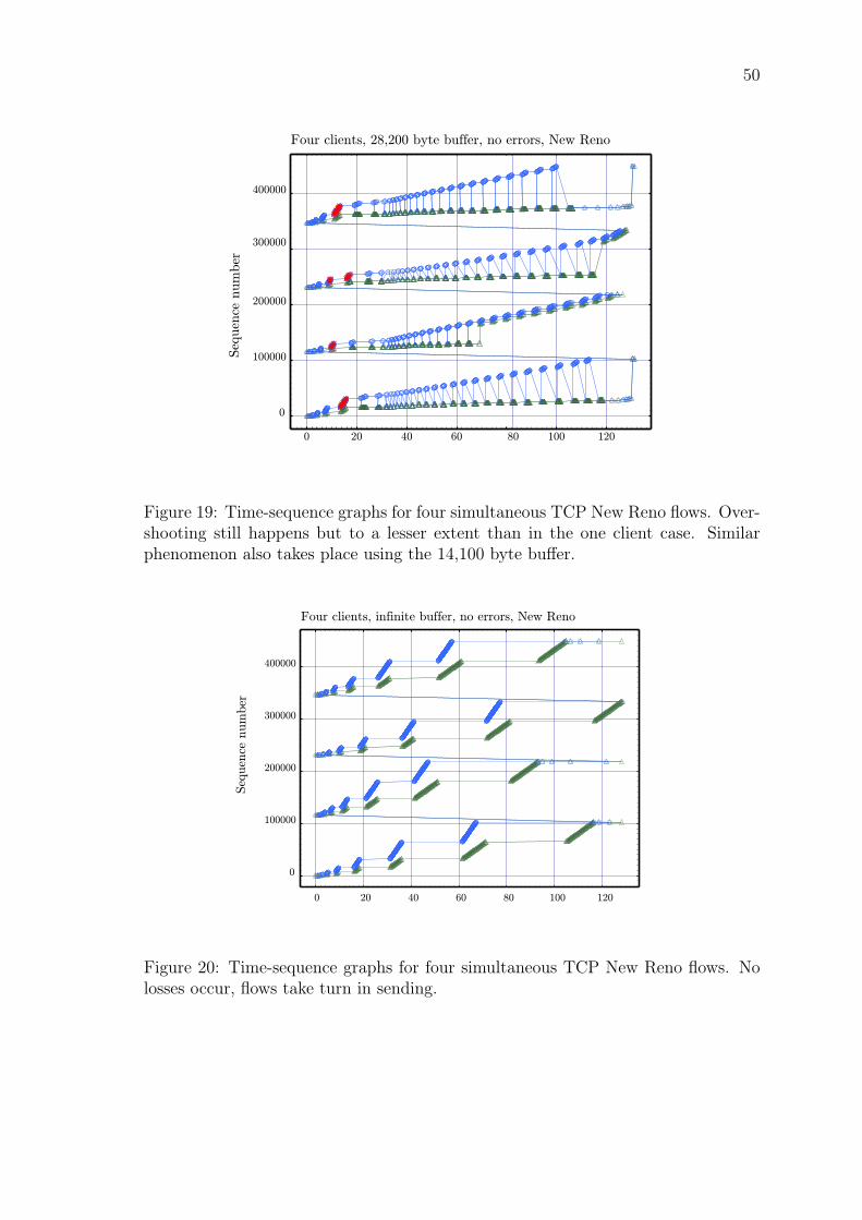
50

0 20 40 60 80 100 120

0

400000

300000

200000

100000

Four clients, 28,200 byte buffer, no errors, New Reno

Seq

uen

ce n

um

ber

Figure 19: Time-sequence graphs for four simultaneous TCP New Reno flows. Over-shooting still happens but to a lesser extent than in the one client case. Similarphenomenon also takes place using the 14,100 byte buffer.

0 20 40 60 80 100 120

0

400000

300000

200000

100000

Four clients, infinite buffer, no errors, New Reno

Seq

uen

ce n

um

ber

Figure 20: Time-sequence graphs for four simultaneous TCP New Reno flows. Nolosses occur, flows take turn in sending.

51

6.2 Error-Prone Link Results

One client, low error rate

The flow completion times for a single client in the low error rate link are shownin Figure 21 with the detailed flow completion times shown in Table 8. The resultsdo not yet differ much from the results of the error-free environment. The medianFCT for Default CoAP is 336 seconds, roughly 10% higher than the median FCT forCoCoA which is 304 seconds. As in the error-free case, both New Reno and BBRhave significantly lower flow completion times than UDP, regardless of the buffersize. The median FCTs for TCP range from 37 to 69 seconds. There is much morevariance between the test runs, but TCP still consistently outperforms the baseline.Even the slowest client—again, one using TCP BBR with the smallest buffer—isable to complete notably faster than any Default CoAP or CoCoA client.

In the error-free link, TCP New Reno exhibited problematic behaviour when themiddle buffers were used. Overshooting in the beginning, it suffered from massivepacket loss. This artefact was especially pronounced in the 28,200 byte buffer. Now,as errors are introduced into the network, the problematic behaviour is preventedbecause early on in the connection some segment is lost. Consequently most TCPNew Reno transfers complete quickly. However, there is one unfortunate case inwhich the first loss occurs quite late. This is why it overshoots in the beginning,repeating the behaviour witnessed in the error-free case. As a result, there is massivepacket loss: altogether 123 segments require retransmitting. For the other test runs,

0

50

100

150

200

250

300

350

400

2500B D

efaultCOAP

2500B C

oCoA

2500B N

ew R

eno

2500B T

CP B

BR

14100B N

ew R

eno

14100B T

CP B

BR

28200B N

ew R

eno

28200B T

CP B

BR

infinite New

Reno

infinite TCP B

BR

Flo

w C

om

ple

tion T

ime

(sec

onds)

Figure 21: The median, minimum, maximum, 25th, and 75th percentiles for oneflow with low error probability and different bottleneck buffer sizes.

52

the number stays well under 50. This case is the one with the highest maximumFCT for any run using TCP, and occurs when the 14,100 byte buffer is used withTCP New Reno. While the other maximum FCT values are close to 60 seconds,this test run takes roughly 90 seconds to complete, so the difference is notable. Atits highest, the RTO timer reaches a value close to 30 seconds, which is high, butstill far from the maximum. The gaps in sending due to the reliance on the RTOtimer explain the notably high FCT.

Otherwise New Reno fares well across the buffers. The median completion time onthe two largest buffers is roughly 42 seconds. There is a small difference of half asecond to the advantage of the infinite buffer—this is the lowest measured medianFCT for New Reno in this setting.

There is not much difference between the results achieved using the second largestand the largest buffer. The slight differences that do exist, are explained by theslightly higher number of lost segments when the smaller buffer is used. Likewise,the differences between the test runs within a buffer are caused by the varyingnumber of lost segments and the differences in when the losses occur.

The difference in the median completion times between New Reno and BBR areroughly 5 to 7 seconds for all the large buffers, with BBR achieving lower values.TCP BBR also achieves very stable results across the buffers, especially when com-pared to New Reno, except with the 2,500 byte buffer. This was the case in theerror-free link, too. The lowest median FCT of all the algorithms and buffers isachieved by TCP BBR: on all buffers but the smallest, the median FCT is close to37 seconds, with the infinite buffer FCT being slightly lower than the FCT for theother two buffers.

Like in the error-free case, the 2,500 byte buffer size proves problematic. ThoughTCP in general is much more efficient than UDP, the median FCT for TCP BBR isnotably high here, almost 70 seconds. Compared with New Reno, in the worst caseit takes more than twice as long for this BBR client to complete. This phenomenonis the same as it was in the error-free setting. If RTO expires, TCP BBR resendsall outstanding segments. In the 2,500 byte buffer RTO expirations happen as BBRis unable to correctly estimate the BDP and so it sends too aggressively, congestingthe link. This is very similar to the phenomenon shown earlier in Figure 17, exceptmuch more pronounced, since now some losses occur also because of link errors.Only five test runs in this setup are faster to complete than the slowest of the NewReno test runs.

Table 8: Flow Completion Time of 1 client with low error rate (seconds)Error-Rate Buffer CC algorithm min 10 25 median 75 90 95 maxlow 2500B DefaultCOAP 311.039 316.381 319.161 336.859 345.589 346.888 349.030 350.080low 2500B CoCoA 297.593 297.899 299.088 304.267 308.842 313.886 316.132 316.991low 2500B New Reno 40.448 41.608 43.166 48.844 56.610 59.681 60.859 62.464low 2500B BBR 42.839 47.385 53.591 69.648 84.973 104.351 127.506 132.084low 14100B New Reno 34.206 34.694 39.792 44.521 54.080 57.299 60.220 90.239low 14100B BBR 34.804 34.856 35.819 37.973 40.465 44.058 49.177 49.391low 28200B New Reno 34.773 36.375 39.820 42.888 51.375 55.159 57.447 61.355low 28200B BBR 34.795 34.856 35.118 37.870 40.391 43.792 49.512 50.903low infinite New Reno 34.209 34.694 38.484 42.432 51.630 56.328 58.812 61.874low infinite BBR 34.721 34.804 35.823 37.048 39.940 41.475 43.920 49.505

53

One client, medium error rate

The flow completion times for one client in the medium error rate link are shownin Figure 22 with the detailed flow completion times shown in Table 9. Where theresults for the low error rate were very similar to the error-free results, here the effectsof the growing error rate start to become visible. The difference between DefaultCoAP and CoCoA grows larger here, with CoCoA being able to benefit better fromits advanced congestion control mechanisms. The median FCT for Default CoAP isroughly 601 seconds, 22% higher than the median FCT of CoCoA. Again, both NewReno and BBR perform better than the baseline but the difference between TCPand UDP is now smaller, especially the difference between New Reno and CoCoA.Compared with TCP, UDP results are more stable—they do not have long tailssuch that BBR or New Reno do on most buffer sizes. Still, the UDP median FCTvalues are notably high. With the exception of the 28,200 byte buffer, New Renomaximum FCT values are lower than the median UDP FCT values. With the twolargest buffer sizes, this is also the case for TCP BBR. However, with the smallestbuffer BBR continues to misbehave. While the median FCT is low, the maximumFCT is notably higher than it is for any other protocol and buffer combination.

Here all the test runs take longer to complete than in the error-free case. For TCPNew Reno, the median FCT values are almost, or over, 200% higher. The differenceis not quite as large for BBR, especially when using the smallest buffer, as its medianFCT was already quite high with the low error rate. For the other buffer sizes themedian BBR FCT values are now very roughly 150% higher. Not surprisingly,

0

500

1000

1500

2000

2500

2500B D

efaultCOAP

2500B C

oCoA

2500B N

ew R

eno

2500B T

CP B

BR

14100B N

ew R

eno

14100B T

CP B

BR

28200B N

ew R

eno

28200B T

CP B

BR

infinite New

Reno

infinite TCP B

BR

Flo

w C

om

ple

tion T

ime

(sec

onds)

Figure 22: The median, minimum, maximum, 25th, and 75th percentiles for oneconcurrent flow with medium error probability and different bottleneck buffer sizes.

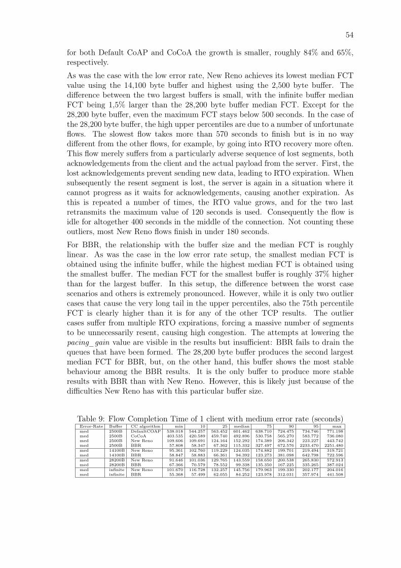
54

for both Default CoAP and CoCoA the growth is smaller, roughly 84% and 65%,respectively.

As was the case with the low error rate, New Reno achieves its lowest median FCTvalue using the 14,100 byte buffer and highest using the 2,500 byte buffer. Thedifference between the two largest buffers is small, with the infinite buffer medianFCT being 1,5% larger than the 28,200 byte buffer median FCT. Except for the28,200 byte buffer, even the maximum FCT stays below 500 seconds. In the case ofthe 28,200 byte buffer, the high upper percentiles are due to a number of unfortunateflows. The slowest flow takes more than 570 seconds to finish but is in no waydifferent from the other flows, for example, by going into RTO recovery more often.This flow merely suffers from a particularly adverse sequence of lost segments, bothacknowledgements from the client and the actual payload from the server. First, thelost acknowledgements prevent sending new data, leading to RTO expiration. Whensubsequently the resent segment is lost, the server is again in a situation where itcannot progress as it waits for acknowledgements, causing another expiration. Asthis is repeated a number of times, the RTO value grows, and for the two lastretransmits the maximum value of 120 seconds is used. Consequently the flow isidle for altogether 400 seconds in the middle of the connection. Not counting theseoutliers, most New Reno flows finish in under 180 seconds.

For BBR, the relationship with the buffer size and the median FCT is roughlylinear. As was the case in the low error rate setup, the smallest median FCT isobtained using the infinite buffer, while the highest median FCT is obtained usingthe smallest buffer. The median FCT for the smallest buffer is roughly 37% higherthan for the largest buffer. In this setup, the difference between the worst casescenarios and others is extremely pronounced. However, while it is only two outliercases that cause the very long tail in the upper percentiles, also the 75th percentileFCT is clearly higher than it is for any of the other TCP results. The outliercases suffer from multiple RTO expirations, forcing a massive number of segmentsto be unnecessarily resent, causing high congestion. The attempts at lowering thepacing_gain value are visible in the results but insufficient: BBR fails to drain thequeues that have been formed. The 28,200 byte buffer produces the second largestmedian FCT for BBR, but, on the other hand, this buffer shows the most stablebehaviour among the BBR results. It is the only buffer to produce more stableresults with BBR than with New Reno. However, this is likely just because of thedifficulties New Reno has with this particular buffer size.

Table 9: Flow Completion Time of 1 client with medium error rate (seconds)Error-Rate Buffer CC algorithm min 10 25 median 75 90 95 maxmed 2500B DefaultCOAP 538.018 544.257 563.452 601.462 638.710 724.475 734.746 771.198med 2500B CoCoA 403.535 420.589 459.740 492.896 530.758 565.270 583.772 736.080med 2500B New Reno 109.606 109.691 124.164 152.292 174.389 206.342 223.227 443.742med 2500B BBR 57.808 58.347 67.362 115.332 327.497 672.576 2233.470 2251.480med 14100B New Reno 95.361 102.760 119.229 124.035 174.882 199.701 219.494 319.721med 14100B BBR 58.847 58.883 66.361 94.392 123.273 381.098 642.798 722.596med 28200B New Reno 91.646 101.036 129.765 143.559 158.650 200.538 265.830 572.913med 28200B BBR 67.366 70.579 78.552 99.338 135.350 167.225 335.265 387.024med infinite New Reno 101.670 116.728 132.257 145.756 179.963 199.330 202.177 204.016med infinite BBR 55.368 57.499 62.055 84.252 123.978 312.031 357.974 441.508

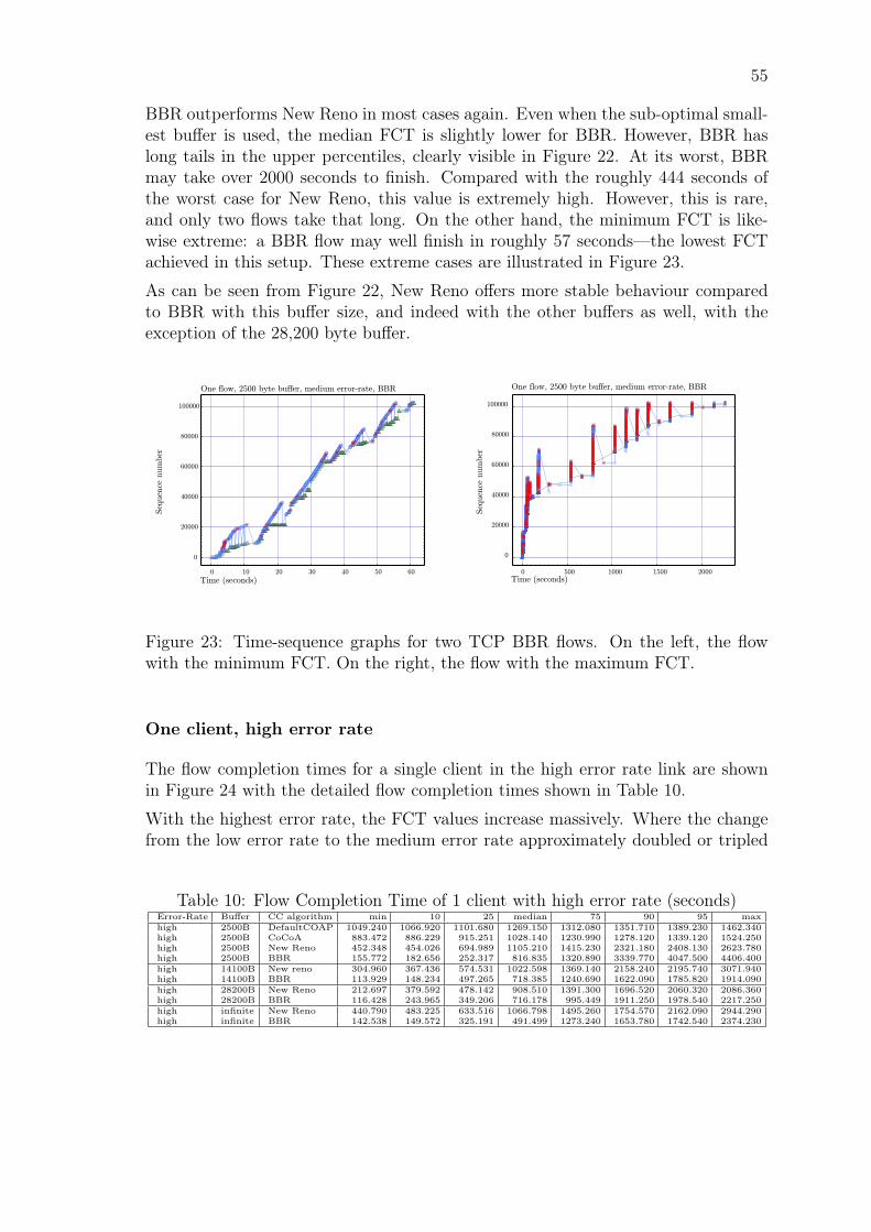
55

BBR outperforms New Reno in most cases again. Even when the sub-optimal small-est buffer is used, the median FCT is slightly lower for BBR. However, BBR haslong tails in the upper percentiles, clearly visible in Figure 22. At its worst, BBRmay take over 2000 seconds to finish. Compared with the roughly 444 seconds ofthe worst case for New Reno, this value is extremely high. However, this is rare,and only two flows take that long. On the other hand, the minimum FCT is like-wise extreme: a BBR flow may well finish in roughly 57 seconds—the lowest FCTachieved in this setup. These extreme cases are illustrated in Figure 23.

As can be seen from Figure 22, New Reno offers more stable behaviour comparedto BBR with this buffer size, and indeed with the other buffers as well, with theexception of the 28,200 byte buffer.

0 10 20 30 40 50 60

0

20000

40000

60000

80000

100000

One flow, 2500 byte buffer, medium error-rate, BBR

Time (seconds)

Seq

uen

ce n

um

ber

0 500 1000 1500 2000

0

20000

40000

60000

80000

Time (seconds)

Seq

uen

ce n

um

ber

100000

One flow, 2500 byte buffer, medium error-rate, BBR

Figure 23: Time-sequence graphs for two TCP BBR flows. On the left, the flowwith the minimum FCT. On the right, the flow with the maximum FCT.

One client, high error rate

The flow completion times for a single client in the high error rate link are shownin Figure 24 with the detailed flow completion times shown in Table 10.

With the highest error rate, the FCT values increase massively. Where the changefrom the low error rate to the medium error rate approximately doubled or tripled

Table 10: Flow Completion Time of 1 client with high error rate (seconds)Error-Rate Buffer CC algorithm min 10 25 median 75 90 95 maxhigh 2500B DefaultCOAP 1049.240 1066.920 1101.680 1269.150 1312.080 1351.710 1389.230 1462.340high 2500B CoCoA 883.472 886.229 915.251 1028.140 1230.990 1278.120 1339.120 1524.250high 2500B New Reno 452.348 454.026 694.989 1105.210 1415.230 2321.180 2408.130 2623.780high 2500B BBR 155.772 182.656 252.317 816.835 1320.890 3339.770 4047.500 4406.400high 14100B New reno 304.960 367.436 574.531 1022.598 1369.140 2158.240 2195.740 3071.940high 14100B BBR 113.929 148.234 497.265 718.385 1240.690 1622.090 1785.820 1914.090high 28200B New Reno 212.697 379.592 478.142 908.510 1391.300 1696.520 2060.320 2086.360high 28200B BBR 116.428 243.965 349.206 716.178 995.449 1911.250 1978.540 2217.250high infinite New Reno 440.790 483.225 633.516 1066.798 1495.260 1754.570 2162.090 2944.290high infinite BBR 142.538 149.572 325.191 491.499 1273.240 1653.780 1742.540 2374.230

56

the median FCT values, here the FCT values are close to being ten times as high.Additionally, here the gap between UDP and TCP narrows notably.

The first observation is, again, that the UDP results are more stable. UDP guar-antees low FCT in the face of high error rate: the worst case scenario FCT valuesfor both CoCoA and Default CoAP are much lower than they are for TCP. On theother hand, UDP is not able to achieve as low completion times as TCP. Addition-ally, median FCT values in general are slightly lower for TCP than UDP with theexception of the CoCoA median FCT being lower than the New Reno median FCTwith the smallest and the largest buffer. The Default CoAP congestion control hasthe highest median FCT in this scenario. New Reno and CoCoA median FCT arevery close to each other while BBR achieves clearly lower values, especially whenusing the infinite buffer. Despite the instability of TCP results, TCP does not per-form altogether badly. Compared to the baseline, most TCP flows are able to finishin a reasonable time, as seen in the 75th percentile results. The 75th percentile flowcompletion times are roughly 11 to 22 percent higher for New Reno than for CoCoA.For BBR, the difference is much smaller. At its lowest, it is under one percent withthe 14,100 byte buffer and, at its highest, seven percent with the 2,500 byte buffer.With the 28,200 byte buffer the 75th percentile FCT is three percent higher forCoCoA than for BBR.

For New Reno, when using the 2,500 byte buffer, altogether five test runs are slowerto finish than the slowest of the Default CoAP flows. These flows exhibit similarpatterns as the outlier flows in the medium error rate environment. Some segments

0

500

1000

1500

2000

2500

3000

3500

4000

4500

2500B D

efaultCOAP

2500B C

oCoA

2500B N

ew R

eno

2500B T

CP B

BR

14100B N

ew R

eno

14100B T

CP B

BR

28200B N

ew R

eno

28200B T

CP B

BR

infinite New

Reno

infinite TCP B

BR

Flo

w C

om

ple

tion T

ime

(sec

onds)

Figure 24: The median, minimum, maximum, 25th, and 75th percentiles for oneflow with high error probability and different bottleneck buffer sizes.

57

are lost so that further segments cannot be sent because of missing acknowledge-ments. Consequently the flows spend long periods of time idle, waiting for the RTOto expire. Often, the RTO reaches the maximum value already quite early on. Ad-ditionally, both the infinite and the 14,100 byte buffer test cases include one test runthat is an extreme outlier, explaining the long tails for those buffers. In the infinitebuffer case, shown in Figure 25, the outlier flow suffers from multiple RTO timeoutsin the very beginning. It loses the first segment it sends after the handshake andimmediately goes into recovery: the retransmitted segment is lost as well. A dupli-cate acknowledgement for it arrives, but because of the delayed acknowledgements,the RTO for the segment expires first. The RTO is not yet very high. However,a previously unacknowledged segment sent during the recovery is lost. The clientsends altogether six acknowledgements for it, but five of them are lost. Thus theserver cannot send the next segment, and has to rely on RTO timeouts for retrans-missions. The flow continues in this way for roughly the first 1,400 seconds. Afterthe flow manages to recover from these first losses, it suffers a few more RTOs, butstill behaves in the same way as the other test runs. The outlier flow in the 14,100byte buffer case shows similar though less extreme behaviour twice during its run.This flow also has the most RTO timeouts out of all the test runs in the 14,100 bytebuffer test case. It should be noted that the maximum RTO for TCP is 120 sec-onds, higher than for Default CoAP and CoCoA, which may, at least partly, explainthe difference in the upper percentiles. When link errors dominate, such high RTOvalues are not optimal.

0 200 400 600 800 1000 1200 1400 1600 1800 2000 2200 2400 2600 2800 3000

0

5000

10000

15000

20000

25000

30000

35000

40000

45000

50000

55000

60000

65000

70000

75000

80000

85000

90000

95000

100000

105000

Seq

uen

ce n

um

ber

One client, 1,410,000 byte buffer, high error rate, NewReno

Figure 25: Time-sequence graph for the slowest TCP New Reno flow using theinfinite buffer in the high error rate environment. The flow is idle for a long periodof time.

58

The median FCT values achieved with TCP New Reno do not fluctuate much frombuffer to buffer. The lowest median FCT is achieved using the 28,200 byte bufferwhile the 2,500 byte buffer produces the highest median FCT for New Reno. The2,500 byte buffer median FCT is 21% higher than the 28,200 byte buffer medianFCT. This seems natural, at least in the sense that the smallest buffer should suffermore congestion-related losses than the larger buffers, in addition to the quite highnumber of losses caused by intermittent errors. In the error-free and low-errorscenarios, the 28,200 byte buffer was not suitable for New Reno. In contrast, here itproduces the overall best results for New Reno. Both the median and the minimumFCT are the lowest achieved by New Reno and the outlier cases are less extreme.The outliers not withstanding, New Reno fares better than Default CoAP and isvery similar to CoCoA. As the plot in Figure 24 shows, 75% of the New Reno flowsfinish in or a little under 1500 seconds, making the majority of the test runs completein roughly similar times.

BBR continues to still show sub-optimal behaviour with the BDP-sized buffer. Whileit does finish faster than New Reno in most cases, three test runs are clearly slower.Compared with New Reno, the BBR results using this buffer are unstable. Thesethree flows have a clearly higher number of lost segments than the other flows. At itslowest, the number of lost segments for the outlier flows is 475: for all other flows thenumber stays below 166. Likewise, these flows require more than 1000 retransmis-sions to finish while the rest of the flows only need at most 500. Supporting this, theLinux kernel TCP metrics show these flows retransmitting more than 600 segmentsduring RTO recovery whereas for other flows only 300 retransmissions take placeduring RTO recovery. However, this metric is not very precise, especially for BBR.The outlier flows tend to start sending earlier, being quicker to finish the handshake.They also send very aggressively already in the beginning. Like the New Reno out-lier flows, sometimes these flows lose multiple acknowledgements, which leads tothe expiration of the RTO timer. BBR then retransmits all unacknowledged data.With the small buffer, the effect is especially detrimental due to the trouble BBRhas estimating the link capacity when the buffers are shallow. It ends up sendingtoo much, making the problem worse as even more segments are dropped. Again,the behaviour of these extreme examples is very similar to the medium error casesshown in Figure 23, except that the effect is more pronounced.

Despite the problematic behaviour of BBR with the small buffer, all the medianFCT values stay clearly under 1000 seconds. Again, the larger buffers are shown tobe most suitable for BBR—the lowest median FCT of this scenario is achieved usingthe infinite buffer. The median FCT of the smallest buffer is 66.2% higher. On theother hand, it has somewhat slower outlier cases than the 28,200 byte buffer, whichreaches slightly lower 75th percentile and maximum FCT values.

BBR has consistently lower median and minimum FCT than New Reno regardlessof the buffer. Despite showing unstable behaviour on the BDP-sized buffer, it nowperforms better compared to New Reno using that buffer than it did when the errorrate was lower. In 75% of the test runs using the smallest buffer BBR flows completeslightly faster than New Reno. Since now New Reno also has long tails in the upper

59

percentiles using the smallest buffer, the difference between the two is diminished.On the larger buffers the difference is completely erased and the tails New Reno hasare longer. Further, New Reno is unable to reach quite as low completion times asBBR. Regardless of the buffer or the error rate, BBR sends more segments in totalthan New Reno. This is explained by it resending all outstanding data upon an RTOexpiration: New Reno retransmit logic is more sophisticated even without selectiveacknowledgements. However, this is not enough to make New Reno altogether moreefficient than BBR.

Four clients, low error rate

The flow completion times of four simultaneous clients in the low error link areshown in Figure 26 with the detailed flow completion times shown in Table 11. Themedian FCT values for TCP are still significantly lower than for UDP. In fact, withthe exception of there being longer tails in both the upper and the lower percentiles,the results are very similar to the error-free case.

Unsurprisingly, the maximum FCT values are now higher than they were in theerror-free setup: roughly 10%, 18%, 19%, and 15%, from the smallest to the largestbuffer, respectively. This showcases the kind of instability that introducing errors tothe network causes, even though the effect is not very dramatic at this low error level.For Default CoAP and CoCoA the relative change is somewhat more moderate, 15%

0

50

100

150

200

250

300

350

400

2500B D

efaultCOAP

2500B C

oCoA

2500B N

ew R

eno

14100B N

ew R

eno

28200B N

ew R

eno

infinite New

Reno

Flo

w C

om

ple

tion T

ime

(sec

onds)

Figure 26: The median, minimum, maximum, 25th, and 75th percentiles for fourconcurrent flows with low error probability and different bottleneck buffer sizes.

60

and 6% respectively. The difference is small because the median FCT was very highin the error-free case, too.

However, for TCP, there are a few interesting observations. First, the infinite buffermedian FCT is 11% higher now than it was when there were no errors—for all theother buffers the difference is very close to one second to either direction. Second,the median FCT of the 28,200 byte buffer is actually slightly higher for the error-freecase. The longer tails are also more pronounced for the 28,200 byte buffer, whichis likely explained by the overshoot behaviour it displayed with the error-free singleclient case.

Third, and more noteworthy, is the observation that now the minimum FCT valuesare lower than they were in the error-free case. For the deeper buffers this is quitenotable: the FCT minima are 50, 97, and 81 percent higher in the error-free casefor the 14,100 byte, 28,200 byte, and the infinite buffers, respectively. That is, thedifference is 38 seconds with the 141,000 byte buffer, 60 seconds with the 28,200byte buffer and 41 with the infinite buffer. For Default CoAP and CoCoA there areno such notable differences. However, the minimum results are of course due to asingle outlier flow. The 10th percentile, meaning two test runs, only shows notabledifference for the middle buffers. For the infinite buffer, the difference is only 7,5percent, while the 10th percentile FCT for the 2,500 byte buffer is lower in the error-free case. Finally, when looking at the 25th percentile, a notable difference existsonly for the infinite buffer, which is 20 seconds, or, roughly 20%, lower for the lowerror case than the error-free case. The overshoot which afflicted the single clienterror-free case does not take place anymore, despite the error rate being low. Thiswas indeed the case with a single client as well: even few errors early on prevent theovershoot behaviour.

The behaviours of the TCP flows in the test runs are very uniform in the case ofthe 2,500 byte buffer. This is also true for most of the runs using the infinite buffer,but roughly half of the infinite buffer test runs include one aggressive flow that isable to finish quickly. This is shown in Figure 27. This phenomenon takes placewhen the other three flows suffer unfortunately timed losses in the very beginning,and consequently are not able to grow their congestion window as quickly as theone lucky flow. When the one flow not suffering from the early drops is able tosend more aggressively, little bandwidth is left for the other flows that then sufferRTOs. In the error-free case, there were no drops when the infinite buffer was used.The clients took turns in sending: each could fully utilise the link for a while whenthe others were waiting for acknowledgements. This phenomenon is prevented bythe drops: now the clients send in a continuous way, occasionally losing one or two

Table 11: Flow Completion Time of four clients with low error rate (seconds)Error-Rate Buffer CC algorithm min 10 25 median 75 90 95 maxlow 2500B DefaultCOAP 301.282 315.217 321.354 327.584 333.751 343.894 349.042 358.129low 2500B CoCoA 292.040 297.829 300.165 303.276 308.191 311.140 312.774 320.116low 2500B CoAPoverTCP 94.996 110.472 119.988 126.763 132.638 137.093 140.320 148.640low 14100B CoAPoverTCP 75.590 97.789 112.165 122.251 131.915 134.896 140.636 149.394low 28200B CoAPoverTCP 62.215 82.883 113.127 126.246 132.409 140.026 143.477 153.626low infinite CoAPoverTCP 50.535 85.503 112.425 121.251 129.525 134.852 137.875 145.880

61

segments. No segments were lost using the infinite buffer whereas some packet lossoccurred using all the other buffers, even in the error-free setup. This explains whythe infinite buffer is the only buffer to have a notably higher median FCT here.For the 28,200 byte buffer, flows that do not suffer early drops have a tendencyto overshoot in the Slow Start and consequently lose many packets in row. This,however, is not very consequential since there is new data to be sent during the FastRecovery.

Despite these phenomena, even in the worst case, TCP is again shown to performvery well compared to UDP. Further, there is not much difference between the buffersizes. The differences of both the median and the maximum FCT values betweenthe buffers stay under 5 seconds.

0 20 40 60 80 100 120 140

0

100000

200000

300000

400000

Four clients, infinite buffer, low error-rate, New Reno

Time (seconds)

Seq

uen

ce n

um

ber

Figure 27: Time-sequence graphs for four simultaneous TCP New Reno flows usingthe infinite buffer. One flow may send aggressively and complete faster than theother three flows.

Four concurrent clients, medium error rate

The flow completion times of 4 simultaneous clients in the medium error rate linkare shown in Figure 28 with the detailed flow completion times shown in Table 12.

As in the single client case, here the difference between UDP and TCP starts togrow smaller. Again, there is very little change for UDP: Default CoAP medianFCT is only 0.7% higher in this case than in the single client case. Also the medianFCT values for TCP are still significantly lower than for UDP. However, the longtails of the TCP results in the upper percentiles exceed the UDP median values,and in the case of the 2,500 byte buffer, even the maximum FCT values.

62

0

100

200

300

400

500

600

700

800

900

2500B D

efaultCOAP

2500B C

oCoA

2500B N

ew R

eno

14100B N

ew R

eno

28200B N

ew R

eno

infinite New

Reno

Flo

w C

om

ple

tion T

ime

(sec

onds)

Figure 28: The median, minimum, maximum, 25th, and 75th percentiles for fourconcurrent flows with medium error probability and different bottleneck buffer sizes.

With this higher error rate, the median FCT and the lower percentiles are verysimilar for TCP across the buffers, but unlike in the low error rate case, there aredifferences in the worst case scenarios.

For New Reno, the two middle-sized buffers achieve the lowest median FCT, butthe difference between them is almost non-existent. Like in the case of the low errorrate, the 2,500 byte buffer median FCT is the highest. There are fewer RTOs inthe 28,200 byte buffer than the 2,500. The total number of timeouts per test runranges from 4 to 16 for the smallest buffer with the median being 11.5. For the2,500 byte buffer case, in 11 out of the 20 test cases, all the flows within a test runbehave similarly. Additionally, five test runs include one flow taking slightly longerthan the others. The rest do not fit this model, and these test runs also include theflows visible in the long tails—both the maximum and minimum values.

Table 12: Flow Completion Time of 4 clients with medium error rate (seconds)Error-Rate Buffer CC algorithm min 10 25 median 75 90 95 maxmed 2500B DefaultCOAP 507.392 547.025 577.940 606.591 651.701 688.765 701.939 761.204med 2500B CoCoA 407.314 435.597 454.252 485.037 515.270 578.340 619.615 730.671med 2500B CoAPoverTCP 114.059 148.351 169.372 198.457 255.709 344.401 400.574 826.577med 14100B CoAPoverTCP 120.564 138.062 157.013 187.923 237.336 327.006 347.524 688.100med 28200B CoAPoverTCP 114.766 141.211 160.975 187.216 234.331 324.613 352.025 584.447med infinite CoAPoverTCP 124.602 140.403 166.157 189.877 233.989 327.948 386.531 653.078

One of the slowest flows of all the flows considered loses three out of four segmentssent in a window right after the handshake. It manages to receive one ACK, butunable to send new data, the RTO expires. This happens a few times during theconnection duration: the receiver is not able to receive enough acknowledgements

63

to trigger a fast retransmit as too many consecutive segments are lost. It cannotsend new data, so it has to rely on the RTO timer, which grows progressively larger.However, the maximum RTO value of 120 seconds is not yet often used here asthe error rate is not yet that high. These cases of unfortunate drop sequences thatlead to the use of RTO instead of duplicate acknowledgements as a loss detectionmechanism explain the differences in the upper percentiles.

Four concurrent clients, high error rate

The flow completion times of 4 simultaneous clients in the high-error link are shownin Figure 29 with the detailed flow completion times shown in Table 13.

When the error rate is at its highest, and there are 4 clients competing for theirshare of the link, the flow completion times explode for all the protocols and buffers.When the error rate was only medium, the maximum FCT of all protocol and buffercombinations stayed under 900 seconds but here the maximum FCT values of TCPare close to 3000 seconds and the UDP maximum FCT is over 1500 seconds. Themedian FCT for UDP is almost doubled. In contrast with the lower error rate cases,there is also a notable increase compared to the single-client high-error case.

A notable observation here is that the difference between the protocols has nowdiminished almost entirely. This also did occur with the single-client high-errorcase. TCP does still achieve lower median FCT than UDP, but it is also more

0

500

1000

1500

2000

2500

3000

2500B D

efaultCOAP

2500B C

oCoA

2500B N

ew R

eno

14100B N

ew R

eno

28200B N

ew R

eno

infinite New

Reno

Flo

w C

om

ple

tion T

ime

(sec

onds)

Figure 29: The median, minimum, maximum, 25th, and 75th percentiles for fourconcurrent flows with high error probability and different bottleneck buffer sizes.

64

unstable as some flows take notably longer to finish than others. UDP does notproduce such outliers.

Default CoAP produces the highest median FCT: roughly 1220 seconds. This is only0,2% higher than in the single-client high-error case. The median values are clearlybetter for TCP than for UDP, while CoCoA and Default CoAP perform similarly.On the other hand, TCP results have long tails. This is partly due to the test setup:the maximum RTO is much higher for TCP than for UDP. As acknowledgements getlost, RTO often dominates as the retransmission trigger, and if it is allowed to growvery large, this leads to long idle periods. As there are many retransmissions, it maybe difficult to get strong samples. Due to Karn’s algorithm, only the strong samplesare taken into account, and consequently TCP may keep a very high, backed-off RTOvalue for a long time. To further accentuate the difference to UDP, the maximumRTO for UDP is lower, so that the idle periods for it are shorter as well. If themaximum RTO used was the same for all the congestion controls, the differencebetween UDP and TCP might be smaller. This is especially true for CoCoA, as italso includes the weak samples into in its RTT estimate.

Here, New Reno does not benefit from the large buffers, except that the results areslightly more uniform using it. New Reno achieves the smallest median FCT usingthe two smallest buffers, with the lowest FCT being achieved using the 14,100 bytebuffer. However, the difference is insignificant, and all the median FCT values arequite close to each other. At this point, there are so many errors that the differencesbetween the buffers seen in the setups with fewer errors are mostly erased.

For the smallest buffer, there is great variability in how the flows behave within atest run. Typically, however, one flow takes notably longer than others. In the worstcase flow, the RTO value very quickly grows to the maximum, 120 seconds. The highRTO value causes long, repeated idle periods when segments or their correspondingacknowledgements are consecutively lost. At times, none of the clients are sendingbecause of this. As an extreme example, one unfortunate segment of this worst-caseflow requires altogether eight transmit attempts. The time elapsed from sendingthe original segment to the first acknowledgement covering it is 8 minutes. Thisis the first such idle period for the flow: time-wise it is not the longest, as theRTO is not yet at 120 seconds for the first few retransmits. But already for thefourth retransmission this maximum value is used. Due to the pattern in which thesegments are lost, this particular flow runs into a similar situation four times, andso takes roughly 48 minutes to finish. This is shown in Figure 30.

For another flow, a similar situation requiring 7 transmit attempts causes an idleperiod of 12 minutes. In contrast, the quickest flow requires only 350 seconds. It is

Table 13: Flow Completion Time of 4 clients with high error rate (seconds)Error-Rate Buffer CC algorithm min 10 25 median 75 90 95 maxhigh 2500B DefaultCOAP 853.327 1008.290 1081.500 1195.690 1338.900 1424.720 1505.240 1562.090high 2500B CoCoA 861.019 933.229 988.545 1125.690 1247.840 1362.670 1404.440 1582.330high 2500B CoAPoverTCP 350.317 467.601 575.476 957.814 1379.940 1722.680 1961.920 2929.610high 14100B CoAPoverTCP 329.074 464.011 593.755 849.291 1226.080 1617.160 1971.760 2477.840high 28200B CoAPoverTCP 358.083 449.452 625.488 980.736 1259.400 1554.140 1749.070 2934.550high infinite CoAPoverTCP 293.360 464.545 627.286 1005.390 1339.050 1710.390 1963.010 2569.410

65

lucky: only 22 segments require retransmitting, and of those only two require fourretransmits. For most segments, one or two retransmits suffice. Maximum RTO isroughly 60 seconds. In this test run, the other two flows take roughly 600 and 1,200seconds while the fourth one takes more than 2,600 seconds so that the pattern ofone flow being notably slower than the others is again observed.

The differences between the flows are due to the way the occurrence of the errors arepatterned: in a lucky flow, the same segment is only lost once or twice. Acknowl-edgements are not dropped, at least not a large part of them, so three duplicateacknowledgements arrive, preventing the slow RTO recovery.

For the 2,500 byte buffer, the small size combined with the higher number of sendersalso causes segments to be dropped due to queue overflow. It can be seen in thatalready in the beginning of the connection, many segments are lost in a short amountof time. For the flows using infinite buffer, the number of segments dropped withinthe first minutes is lower. On the other hand, the deep buffer may also cause longqueuing delays, making the flows in general take longer. The middle-sized bufferslikely offer a working balance between the two extremes.

Interestingly, for New Reno, the median FCT for 1 client is higher than for fourclients, except when the 28,200 buffer is used. For the 2,500 byte, 14,100 byte, andthe infinite buffer the differences are roughly 15%, 22%, and 6% respectively, so thatthe single client FCT is higher. The four client case median FCT of 28,200 bytebuffer is roughly 8% higher. Notably this buffer size was clearly most suitable for

0 500 1000 1500 2000 2500 3000

0

100000

200000

300000

400000

Seq

uen

ce n

um

ber

Four clients, 2500 byte buffer, high error-rate, New Reno

Figure 30: Time-sequence graph for four simultaneous TCP New Reno flows. Oneflow waits for an acknowledgement repeatedly, altogether for more than eight min-utes.

66

New Reno in the one client case, outperforming the others both when judging by themedian an the upper percentiles. This phenomenon is somewhat unnatural—moretraffic in the link should increase the number of lost segments and make the flowscomplete slower because of the need to retransmit so many segments. This couldpartly be explained by the metric itself. When only a single flow is using the link,the timing and pacing of the errors may affect the flow significantly: in a lucky casethe flow is not much bothered by them, in an unlucky case the flow is constantlywaiting for the RTO timer that has reached the maximum value. On the otherhand, when there are four flows, typically only one of them is unlucky in such away: the other four may complete notably fast. As the FCT metric only considerssingle flows and not entire test runs, these lucky flows may come to dominate eventhe middle percentiles. However, in this case the maximum FCT values should stillbe higher in the four client case, but this is true for the 2,500 byte and 28,200 bytebuffers only.

6.3 Summary

In the error-free setting, with only one client, TCP completion time is very closeto ideal, showing it can efficiently fill the link. In contrast, in the same scenario,Default CoAP and CoCoA are only able to use a portion of all the available capacityof the link. This is demonstrated by the stability of the UDP results. As the numberof clients is increased to four, Default CoAP and CoCoA show little change fromthe single client case, regardless of the error rate. Both are severely limited bytheir back-to-back approach: they may only have one message in flight at a time.A larger NSTART value has been shown to increase efficiency by allowing moredata in-flight, but this approach is not scalable, as it does not react to perceivedchanges in the network. TCP, on the other hand, reacts to higher traffic as expected.When the number of concurrent clients is increased to four, median FCT becomesroughly two times higher, both in the error-free and low- error settings. However,the difference between the one and four client cases becomes less visible as error rategrows to medium and beyond. With high error rate, the errors dominate so muchthat differences between the one and four client cases are erased.

The difference between UDP and TCP is at its greatest when there are no or fewerrors. In high-error settings, the difference between UDP and TCP diminishes. Themedian FCT values become very similar, and additionally certain test runs usingTCP take notably long to finish. These outliers are explained by a few recurring phe-nomena. First, New Reno suffers massive losses when using the middle-sized buffers.This is an artefact due to the way the workload and the buffers are configured. TCPNew Reno clients overshoot in Slow Start, lose a significant number of segments, andcannot benefit from the possibility to send new data during Fast Retransmit. This isespecially pronounced with the 28,200 byte buffer but also happens with the 14,100buffer. Second, BBR fails to properly estimate the link capacity when the smallestbuffer is used. BBR flows continuously send too aggressively, fail to drain the linkin Probe RTT, and run into RTOs which make them resend all unacknowledged

67

segments—a large portion of them unnecessarily. Finally, both TCP variants alsosuffer unlucky sequences of lost segments that hinder the flows. A typical conse-quence for New Reno is repeated RTOs. As the RTO value reaches a high value, theflow may spend long periods of time idle, waiting for the RTO to expire. However,despite these phenomena, the median FCT values for TCP are lower in all the four-client test cases and those one-client cases where the error rate is below high. In thehigh-error single-client case, New Reno median FCT is lower than Default CoAPFCT and very close to CoCoA, while BBR achieves clearly lower FCT values. BBRalso proved to be robust in face of high error rate and bufferbloat, outperformingNew Reno in almost all scenarios, despite its difficulties with the bandwidth-delayproduct sized buffer. These problems may be attributed to the non-standard config-uration of the host, namely, the disabling of selective acknowledgements. However,constrained devices might not be able to run a full TCP/IP stack that implementsall TCP extensions. Thus hosts communicating with constrained devices should beable to work with a minimal TCP implementation.

68

7 Conclusion

The Internet of Things consists of various objects that are typically less capable thanregular, modern Internet nodes, for example due to limited memory and processingpower, and because they often use low-speed links prone to errors. The ConstrainedApplication Protocol (CoAP) is a lightweight resource manipulation protocol specif-ically designed for constrained settings. By default, the transport layer for CoAPis UDP. Due to its connectionless nature and low overhead, UDP is well-suited fortypical IoT traffic consisting of intermittent exchanges of short messages

However, IoT devices may also need to transfer large amounts of data, for exampleto perform firmware updates. Further, the number of IoT devices is expected togrow, and since IoT devices partake in the global Internet, IoT protocols need tobe congestion-safe. CoAP implements a straightforward congestion control mecha-nism, but it has been shown to be vulnerable to congestion collapse. In contrast,TCP congestion control is robust and well-understood. RFC 8323 specifies how tocarry CoAP over reliable, stateful protocols, including TCP. As the specification isrelatively new, little research exists.

This work showed CoAP over TCP to be an efficient and scalable choice for long-lived connections in a constrained setting. Changes in the network were reflectedin TCP behaviour: TCP was found to better utilise the capacity of the link whenerrors were infrequent, even in the presence of congestion and bufferbloat. TCPflows also clearly slowed down as the traffic level was increased. In contrast, CoAPover UDP was not scalable in this sense. UDP flows were slow to complete when thelink was good, and as the traffic level grew, they showed little change, as expected.

On the other hand, in high-error settings, regardless of the traffic level, TCP be-haviour was shown to be unstable: some TCP flows were extremely slow to complete.In contrast, UDP behaved predictably, and the differences between the slow and thefast flows were much smaller than they were for TCP. However, the extremely slowflows were mere outliers explained by unfortunately timed losses, and most TCPflows were faster than UDP flows. Some TCP flows reached notably low completiontimes, and clearly outperformed all UDP flows.

This thesis also evaluated the performance of TCP BBR, finding it a promisingcandidate for TCP congestion control. However, some shortcomings were found,motivating further research. These included problems in the Linux kernel BBRimplementation as well as confirming the previous finding that TCP BBR has troubleadjusting its send rate to buffer sizes smaller than or equal to the bandwidth-delayproduct of the link. When such a buffer was used, BBR behaved erratically, leadingto some BBR flows being extremely slow. In the error-free and low-error setting,when this buffer size was used, New Reno outperformed BBR. Otherwise, BBRoutperformed New Reno, and was shown to be both error-tolerant and efficient inthe presence of bufferbloat.

Previous work shows that for very short connections, when the link is prone toerrors, the header overhead may grow too large. However, this work shows that

69

when connections are long-lived, carrying CoAP over TCP is beneficial. TCP isable to react to losses in a sophisticated way, utilising link capacity to the fullestwhen there are no errors or congestion, while also being able to reduce the sendrate in face of congestion. In contrast, both the Default CoAP congestion controland CoCoA were shown to be inefficient when the amount of data to transfer islarge. This work also showed TCP BBR to be efficient in a high-error environmentwith bufferbloat, clearly outperforming both UDP and TCP New Reno. While NewReno occasionally struggled with the large buffers, BBR avoided such problems bymore accurately estimating the link capacity. Default CoAP may be useful in veryconstrained devices that exchange messages infrequently, but if a large amount ofdata needs to be transferred and the expected traffic level is high, carrying CoAPtraffic over the robust and well-understood TCP is an efficient choice.

70

References

ABF01 M. Allman, H. Balakrishnan and S. Floyd, Enhancing TCP’s Loss RecoveryUsing Limited Transmit. rfc 3042, January 2001.

AFP02 M. Allman, S. Floyd and C. Partridge, Increasing TCP’s Initial Window.rfc 3390, November 2002.

AIM10 L. Atzori, A. Iera and G. Morabito, The Internet of Things: A survey.Computer Networks, 54,15(2010), pages 2787 – 2805.

Ake95 S. Akesson, GPRS, general packet radio service. International Conferenceon Universal Personal Communications. IEEE, Nov 1995, pages 640–643.

APB09 M. Allman, V. Paxson and E. Blanton, TCP Congestion Control. rfc 5681,September 2009.

ASHA18 G. A. Akpakwu, B. J. Silva, G. P. Hancke and A. M. Abu-Mahfouz, ASurvey on 5G Networks for the Internet of Things: Communication Technologiesand Challenges. IEEE Access, 6, pages 3619–3647.

BBCM99 L. Brignol, J. Brouet, P. Charriere and F. Mercier, Effects of traffic char-acteristics on the General Packet Radio Service (GPRS) performance. VehicularTechnology Conference, volume 2. IEEE, 1999, pages 844–848.

BBGD18 C. Bormann, A. Betzler, C. Gomez and I. Demirkol, CoAP SimpleCongestion Control/Advanced. Internet Draft, February 2018. URL https://tools.ietf.org/html/draft-ietf-core-cocoa-03. Work in progress.

BBJS14 D. Borman, B. Braden, V. Jacobson and R. Scheffenegger, TCP Extensionsfor High Performance. rfc 7323, September 2014.

BEK14 C. Bormann, M. Ersue and A. Keranen, Terminology for Constrained-NodeNetworks. rfc 7228, May 2014.

BGDK14 A. Betzler, C. Gomez, I. Demirkol and M. Kovatsch, Congestion Controlfor CoAP Cloud Services. Conference on Emerging Technology and FactoryAutomation. IEEE, September 2014, pages 1–6.

BGDP13 A. Betzler, C. Gomez, I. Demirkol and J. Paradells, Congestion Control inReliable CoAP Communication. International Conference on Modeling, Analysisand Simulation of Wireless and Mobile Systems. ACM, 2013, pages 365–372.

BGDP15 A. Betzler, C. Gomez, I. Demirkol and J. Paradells, CoCoA+: An Ad-vanced Congestion Control Mechanism for CoAP. Ad Hoc Networks, 33, pages126–139.

BGDP16 A. Betzler, C. Gomez, I. Demirkol and J. Paradells, CoAP congestioncontrol for the internet of things. IEEE Communications Magazine, 54,7(2016),pages 154–160.

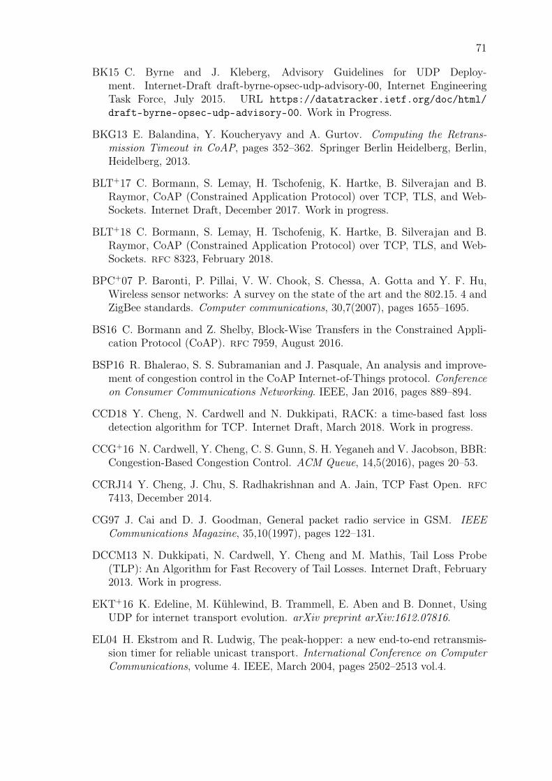
71

BK15 C. Byrne and J. Kleberg, Advisory Guidelines for UDP Deploy-ment. Internet-Draft draft-byrne-opsec-udp-advisory-00, Internet EngineeringTask Force, July 2015. URL https://datatracker.ietf.org/doc/html/draft-byrne-opsec-udp-advisory-00. Work in Progress.

BKG13 E. Balandina, Y. Koucheryavy and A. Gurtov. Computing the Retrans-mission Timeout in CoAP, pages 352–362. Springer Berlin Heidelberg, Berlin,Heidelberg, 2013.

BLT+17 C. Bormann, S. Lemay, H. Tschofenig, K. Hartke, B. Silverajan and B.Raymor, CoAP (Constrained Application Protocol) over TCP, TLS, and Web-Sockets. Internet Draft, December 2017. Work in progress.

BLT+18 C. Bormann, S. Lemay, H. Tschofenig, K. Hartke, B. Silverajan and B.Raymor, CoAP (Constrained Application Protocol) over TCP, TLS, and Web-Sockets. rfc 8323, February 2018.

BPC+07 P. Baronti, P. Pillai, V. W. Chook, S. Chessa, A. Gotta and Y. F. Hu,Wireless sensor networks: A survey on the state of the art and the 802.15. 4 andZigBee standards. Computer communications, 30,7(2007), pages 1655–1695.

BS16 C. Bormann and Z. Shelby, Block-Wise Transfers in the Constrained Appli-cation Protocol (CoAP). rfc 7959, August 2016.

BSP16 R. Bhalerao, S. S. Subramanian and J. Pasquale, An analysis and improve-ment of congestion control in the CoAP Internet-of-Things protocol. Conferenceon Consumer Communications Networking. IEEE, Jan 2016, pages 889–894.

CCD18 Y. Cheng, N. Cardwell and N. Dukkipati, RACK: a time-based fast lossdetection algorithm for TCP. Internet Draft, March 2018. Work in progress.

CCG+16 N. Cardwell, Y. Cheng, C. S. Gunn, S. H. Yeganeh and V. Jacobson, BBR:Congestion-Based Congestion Control. ACM Queue, 14,5(2016), pages 20–53.

CCRJ14 Y. Cheng, J. Chu, S. Radhakrishnan and A. Jain, TCP Fast Open. rfc7413, December 2014.

CG97 J. Cai and D. J. Goodman, General packet radio service in GSM. IEEECommunications Magazine, 35,10(1997), pages 122–131.

DCCM13 N. Dukkipati, N. Cardwell, Y. Cheng and M. Mathis, Tail Loss Probe(TLP): An Algorithm for Fast Recovery of Tail Losses. Internet Draft, February2013. Work in progress.

EKT+16 K. Edeline, M. Kühlewind, B. Trammell, E. Aben and B. Donnet, UsingUDP for internet transport evolution. arXiv preprint arXiv:1612.07816.

EL04 H. Ekstrom and R. Ludwig, The peak-hopper: a new end-to-end retransmis-sion timer for reliable unicast transport. International Conference on ComputerCommunications, volume 4. IEEE, March 2004, pages 2502–2513 vol.4.

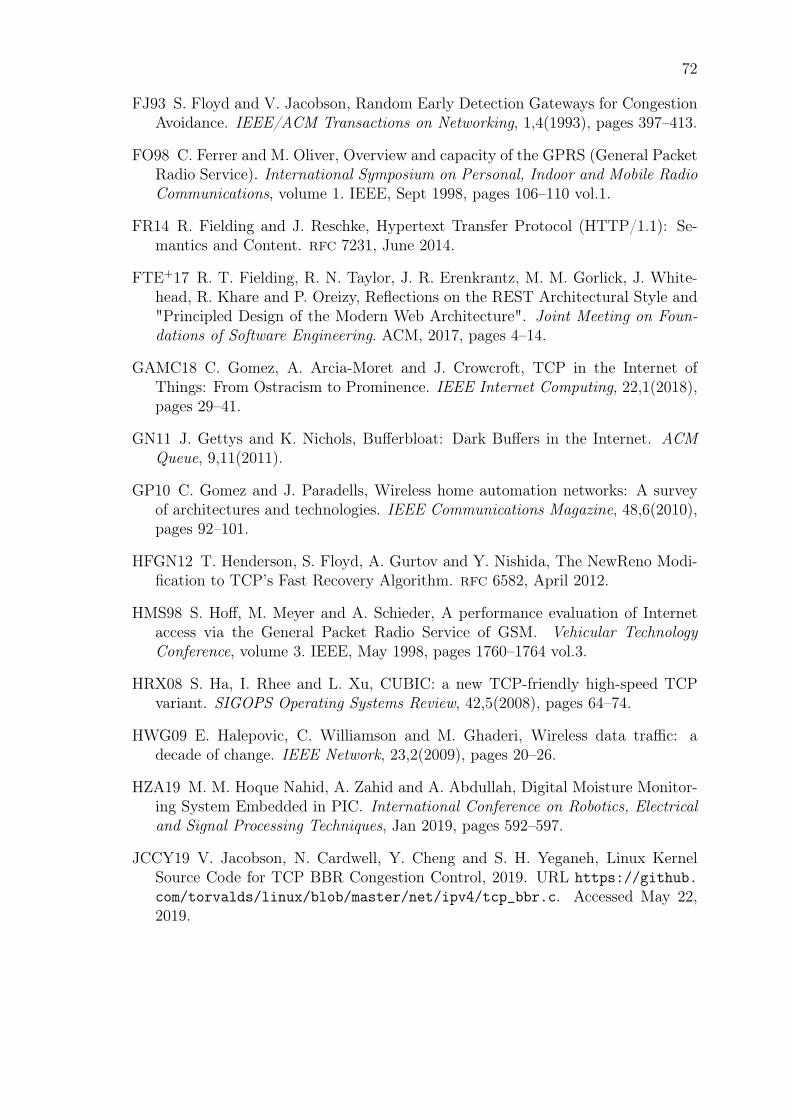
72

FJ93 S. Floyd and V. Jacobson, Random Early Detection Gateways for CongestionAvoidance. IEEE/ACM Transactions on Networking, 1,4(1993), pages 397–413.

FO98 C. Ferrer and M. Oliver, Overview and capacity of the GPRS (General PacketRadio Service). International Symposium on Personal, Indoor and Mobile RadioCommunications, volume 1. IEEE, Sept 1998, pages 106–110 vol.1.

FR14 R. Fielding and J. Reschke, Hypertext Transfer Protocol (HTTP/1.1): Se-mantics and Content. rfc 7231, June 2014.

FTE+17 R. T. Fielding, R. N. Taylor, J. R. Erenkrantz, M. M. Gorlick, J. White-head, R. Khare and P. Oreizy, Reflections on the REST Architectural Style and"Principled Design of the Modern Web Architecture". Joint Meeting on Foun-dations of Software Engineering. ACM, 2017, pages 4–14.

GAMC18 C. Gomez, A. Arcia-Moret and J. Crowcroft, TCP in the Internet ofThings: From Ostracism to Prominence. IEEE Internet Computing, 22,1(2018),pages 29–41.

GN11 J. Gettys and K. Nichols, Bufferbloat: Dark Buffers in the Internet. ACMQueue, 9,11(2011).

GP10 C. Gomez and J. Paradells, Wireless home automation networks: A surveyof architectures and technologies. IEEE Communications Magazine, 48,6(2010),pages 92–101.

HFGN12 T. Henderson, S. Floyd, A. Gurtov and Y. Nishida, The NewReno Modi-fication to TCP’s Fast Recovery Algorithm. rfc 6582, April 2012.

HMS98 S. Hoff, M. Meyer and A. Schieder, A performance evaluation of Internetaccess via the General Packet Radio Service of GSM. Vehicular TechnologyConference, volume 3. IEEE, May 1998, pages 1760–1764 vol.3.

HRX08 S. Ha, I. Rhee and L. Xu, CUBIC: a new TCP-friendly high-speed TCPvariant. SIGOPS Operating Systems Review, 42,5(2008), pages 64–74.

HWG09 E. Halepovic, C. Williamson and M. Ghaderi, Wireless data traffic: adecade of change. IEEE Network, 23,2(2009), pages 20–26.

HZA19 M. M. Hoque Nahid, A. Zahid and A. Abdullah, Digital Moisture Monitor-ing System Embedded in PIC. International Conference on Robotics, Electricaland Signal Processing Techniques, Jan 2019, pages 592–597.

JCCY19 V. Jacobson, N. Cardwell, Y. Cheng and S. H. Yeganeh, Linux KernelSource Code for TCP BBR Congestion Control, 2019. URL https://github.com/torvalds/linux/blob/master/net/ipv4/tcp_bbr.c. Accessed May 22,2019.

73

JDK15 I. Järvinen, L. Daniel and M. Kojo, Experimental Evaluation of AlternativeCongestion Control Algorithms for Constrained Application Protocol (CoAP).World Forum on Internet of Things. IEEE, December 2015.

JKRC18 I. Järvinen, M. Kojo, I. Raitahila and Z. Cao, Fast-Slow Retransmissionand Congestion Control Algorithm for CoAP. Internet Draft, June 2018. Workin progress.

JPR+18 I. Järvinen, L. Pesola, I. Raitahila, Z. Cao and M. Kojo, Performance Eval-uation of Constrained Application Protocol over TCP. IEEE Vehicular Technol-ogy Conference, Aug 2018, pages 1–7.

JRCK18a I. Järvinen, I. Raitahila, Z. Cao and M. Kojo, FASOR RetransmissionTimeout and Congestion Control Mechanism for CoAP. Conference on GlobalCommunications. IEEE, December 2018, pages 1–7.

JRCK18b I. Järvinen, I. Raitahila, Z. Cao and M. Kojo, Is CoAP Congestion Safe?Proceedings of the Applied Networking Research Workshop 2018. ACM, July2018, pages 43–49.

KMS07 N. Kushalnagar, G. Montenegro and C. Schumacher, IPv6 over Low-PowerWireless Personal Area Networks (6LoWPANs): Overview, Assumptions, Prob-lem Statement, and Goals. rfc 4919, August 2007.

KP87 P. Karn and C. Partridge, Improving Round-trip Time Estimates in Reli-able Transport Protocols. Workshop on Frontiers in Computer CommunicationsTechnology. ACM, August 1987, pages 2–7.

LDXZ18 S. Li, L. Da Xu and S. Zhao, 5G Internet of Things: A survey. Journal ofIndustrial Information Integration, 10, pages 1–9.

libcoap libcoap: C-Implementation of CoAP. URL https://libcoap.net/.

LNV+17 M. Lauridsen, H. Nguyen, B. Vejlgaard, I. Z. Kovacs, P. Mogensen and M.Sorensen, Coverage Comparison of GPRS, NB-IoT, LoRa, and SigFox in a 7800km2 Area. Vehicular Technology Conference. IEEE, 2017.

MDC13 M. Mathis, N. Dukkipati and Y. Cheng, Proportional Rate Reduction forTCP. rfc 6937, May 2013.

MHT07 L. Mamatas, T. Harks and V. Tsaoussidis, Approaches to congestion controlin packet networks. Journal of Internet Engineering, 1,1(2007).

MMFR96 M. Mathis, J. Mahdavi, S. Floyd and A. Romanow, TCP Selective Ac-knowledgment Options. rfc 2018, October 1996.

MNY+18 C. Mouradian, D. Naboulsi, S. Yangui, R. H. Glitho, M. J. Morrow andP. A. Polakos, A Comprehensive Survey on Fog Computing: State-of-the-Artand Research Challenges. IEEE Communications Surveys Tutorials, 20,1(2018),pages 416–464.

74

MPV11 L. Mainetti, L. Patrono and A. Vilei, Evolution of wireless sensor networkstowards the Internet of Things: A survey. International Conference on Software,Telecommunications and Computer Networks. IEEE, Sep. 2011, pages 1–6.

Nag84 J. Nagle, Congestion Control in IP/TCP Internetworks. rfc 896, January1984.

NJ12 K. Nichols and V. Jacobson, Controlling Queue Delay. ACM Queue,10,5(2012).

NV19 T. P. Nam and N. Van Doai, Application of Intelligent Lighting Controlfor Street Lighting System. International Conference on System Science andEngineering. IEEE, July 2019, pages 53–56.

OZH07 A. Othman, M. Zakaria and K. A. Hamid, TCP performance measurementin different GPRS network scenarios. Asia-Pacific Conference on Applied Elec-tromagnetics. IEEE, 2007, pages 1–5.

PA00 V. Paxson and M. Allman, Computing TCP’s Retransmission Timer. rfc2988, November 2000.

PACS11 V. Paxson, M. Allman, J. Chu and M. Sargent, Computing TCP’s Re-transmission Timer. rfc 6298, June 2011.

Pos80 J. Postel, User Datagram Protocol. rfc 768, August 1980.

Pos81 J. Postel, Transmission Control Protocol. rfc 793, September 1981.

Rai19 I. Raitahila, Congestion Control Algorithms for the Constrained ApplicationProtocol (CoAP). Master’s thesis, University of Helsinki, 2019.

RAVX+16 A. Rico-Alvarino, M. Vajapeyam, H. Xu, X. Wang, Y. Blankenship, J.Bergman, T. Tirronen and E. Yavuz, An overview of 3GPP enhancements on ma-chine to machine communications. IEEE Communications Magazine, 54,6(2016),pages 14–21.

RFB01 K. Ramakrishnan, S. Floyd and D. Black, The Addition of Explicit Conges-tion Notification (ECN) to IP. rfc 3168, September 2001.

RJR16 S. Ray, Y. Jin and A. Raychowdhury, The Changing Computing ParadigmWith Internet of Things: A Tutorial Introduction. IEEE Design Test, 33,2(2016),pages 76–96.

RXH+18 I. Rhee, L. Xu, S. Ha, A. Zimmermann, L. Eggert and R. Scheffenegger,CUBIC for Fast Long-Distance Networks. rfc 8312, February 2018.

SHB14 Z. Shelby, K. Hartke and C. Bormann, The Constrained Application Proto-col (CoAP). rfc 7252, June 2014.

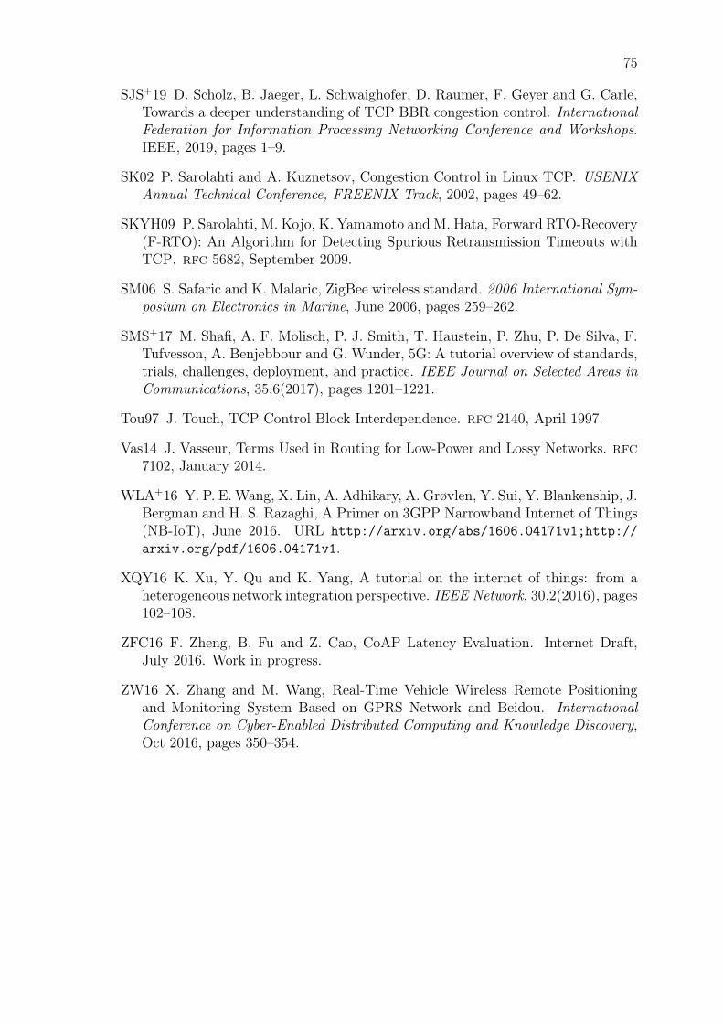
75

SJS+19 D. Scholz, B. Jaeger, L. Schwaighofer, D. Raumer, F. Geyer and G. Carle,Towards a deeper understanding of TCP BBR congestion control. InternationalFederation for Information Processing Networking Conference and Workshops.IEEE, 2019, pages 1–9.

SK02 P. Sarolahti and A. Kuznetsov, Congestion Control in Linux TCP. USENIXAnnual Technical Conference, FREENIX Track, 2002, pages 49–62.

SKYH09 P. Sarolahti, M. Kojo, K. Yamamoto and M. Hata, Forward RTO-Recovery(F-RTO): An Algorithm for Detecting Spurious Retransmission Timeouts withTCP. rfc 5682, September 2009.

SM06 S. Safaric and K. Malaric, ZigBee wireless standard. 2006 International Sym-posium on Electronics in Marine, June 2006, pages 259–262.

SMS+17 M. Shafi, A. F. Molisch, P. J. Smith, T. Haustein, P. Zhu, P. De Silva, F.Tufvesson, A. Benjebbour and G. Wunder, 5G: A tutorial overview of standards,trials, challenges, deployment, and practice. IEEE Journal on Selected Areas inCommunications, 35,6(2017), pages 1201–1221.

Tou97 J. Touch, TCP Control Block Interdependence. rfc 2140, April 1997.

Vas14 J. Vasseur, Terms Used in Routing for Low-Power and Lossy Networks. rfc7102, January 2014.

WLA+16 Y. P. E. Wang, X. Lin, A. Adhikary, A. Grøvlen, Y. Sui, Y. Blankenship, J.Bergman and H. S. Razaghi, A Primer on 3GPP Narrowband Internet of Things(NB-IoT), June 2016. URL http://arxiv.org/abs/1606.04171v1;http://arxiv.org/pdf/1606.04171v1.

XQY16 K. Xu, Y. Qu and K. Yang, A tutorial on the internet of things: from aheterogeneous network integration perspective. IEEE Network, 30,2(2016), pages102–108.

ZFC16 F. Zheng, B. Fu and Z. Cao, CoAP Latency Evaluation. Internet Draft,July 2016. Work in progress.

ZW16 X. Zhang and M. Wang, Real-Time Vehicle Wireless Remote Positioningand Monitoring System Based on GPRS Network and Beidou. InternationalConference on Cyber-Enabled Distributed Computing and Knowledge Discovery,Oct 2016, pages 350–354.