an experimental study of roman dropshaft operation : hydraulics, two-phase … · · 2016-08-08an...

AN EXPERIMENTAL STUDY OF ROMAN DROPSHAFT OPERATION : HYDRAULICS, TWO-PHASE FLOW, ACOUSTICS

by

Hubert CHANSON M.E., ENSHM Grenoble, INSTN, PhD (Cant.), DEng (Qld)

Eur.Ing., MIEAust., MIAHR Reader in Environmental Fluid Mechanics and Water Engineering

Dept of Civil Engineering, The University of Queensland, Brisbane QLD 4072, Australia Email: mailto:[email protected]

Url : http://www.uq.edu.au/~e2hchans/

REPORT No. CH 50/02 ISBN 1864996544

Department of Civil Engineering The University of Queensland

December, 2002

Prototype P2 in operation with a regime R3a

ii

Synopsis : A Dropshaft is an energy dissipator connecting two channels with different invert elevations. In the present study, the hydraulics of vertical, rectangular dropshafts was systematically investigated in two prototypes and five smaller models. Experimental observations showed three basic flow regimes for dropshaft configurations with 180 degree outflow direction. For dropshaft configurations with 90 degree outflow direction, only two flow regimes were observed. At low flow rates, the rate of energy dissipation in the dropshafts was nearly 95%. In the models, the pool depth had little effects on the hydraulic properties of the dropshaft, but larger rate of energy dissipation was consistently observed with 90º outflow direction. Neutrally-buoyant particles were used to record particle residence times in the shafts. For low flow rates and deep shaft pools, the probability distribution functions of residence times exhibited a bi-modal distribution in both model and prototype. Detailed air-water flow and acoustic measurements were conducted in one prototype dropshaft under controlled flow conditions. Void fraction measurements demonstrated a strong aeration of the shaft pool for all flow regimes, but regime R2. The air-water content distributions were basically two-dimensional . At low flow rates, the data were successively compared with an analytical solution of the air bubble advective diffusion equation. Pseudo-bubble chord size measurements showed a broad range of entrained bubble sizes, from less than 0.5 mm to more than 25 mm, with mean pseudo-bubble chords between 10 and 20 mm. The distributions of chord sizes were skewed with a preponderance of small bubbles compared to the mean. Analysis of the streamwise distributions of bubbles indicated a fair proportion of bubbles associated with a cluster structure and the large majority of clusters consisted of 2 bubbles only. Acoustic signatures of the bubbly flow characterised accurately the changes in flow regimes. However the transformation from acoustic frequencies to bubble radii underestimated the entrained bubble sizes and it did not predict the shape of bubble size probability distribution functions measured with intrusive conductivity probes. Although basic hydraulic characteristics were similar between model and prototype based upon a Froude similitude, observations of dimensionless bubble penetration depths and neutrally-buoyant particle residence times showed some discrepancies between model and prototype results. It is believed that these differences highlight the limitations of a Froude similitude for studies of air entrainment, residence times and mass transfer in dropshaft even with a geometric scaling ratio LR = 3.1 as in the present work.

iii

TABLE OF CONTENTS

Page

Synopsis ii

Table of contents iii

Notation iv

About the writer vii

1. Introduction 1

2. Experimental setup

3. Flow patterns

4. Hydraulic properties

5. Particle residence times

6. Air-water flow properties

7. Acoustic characteristics of the shaft

8. Discussion : Roman dropshaft design

9. Conclusion

Acknowledgments

APPENDICES

Appendix A. Jet trajectory calculations : application to dropshaft operation A-1

Appendix B. Experimental results (1) Hydraulic performances A-5

Appendix C. Experimental results (2) Particle residence times A-8

Appendix D. Experimental results (3) Void fractions and bubble count rates A-16

Appendix E. Experimental results (4) Bubble chord time distributions A-24

Appendix F. Bubble clustering analysis A-31

Appendix G. Acoustic data analysis A-33

References R-1

Internet references R-3

Bibliographic reference R-5

iv

NOTATION ao Minnaert factor (m/s) (Eq. (7-2)); B dropshaft width (m); b open channel width (m); C air concentration defined as the volume of air per unit volume of air and water; it is also called

void fraction; Cmax maximum air concentration in the air bubble diffusion layer; Cp specific heat at constant pressure (J/kg.K); Cv specific heat at constant volume (J/kg.K); ch chord length (m); chab pseudo bubble chord length (m) : chab = Vi * tch; chw pseudo water chord size (m); D 1- conduit diameter (m); 2- conduit height (m); Dab bubble penetration depth (m) measured vertically from the free-surface; Dt turbulent diffusivity (m2/s) of air bubbles in two-dimensional plunging jet flow; D# dimensionless turbulent diffusivity for two-dimensional plunging jets; D* dimensionless turbulent diffusivity for circular plunging jets; d flow depth (m) measured perpendicular to the channel bed; db brink depth (m) : i.e., depth at the edge of a drop;

dc critical flow depth (m); in a rectangular channel : dc = 3

q2/g;

di nappe thickness (m) at impact : i.e., thickness of the free-falling jet at impact; F air bubble count rate (Hz) defined as the number of detected air bubbles divided by the scanning

time; Fmax maximum bubble count rate (Hz) at a given cross-section; Fr Froude number; for a rectangular channel : Fr = V/ g*d = Q/ g*d3*b2 ; g gravity constant (m/s2); g = 9.80 m/s2 in Brisbane; H total head (m); H2 residual head (m) : H2 = H1 - ∆H; H1 upstream total head (m); h drop (m) in invert elevation; L dropshaft length (m); LR geometric scaling ratio : i.e., ratio of prototype to model dimensions; l brink overhanging (m) over the shaft; P (shaft) pool height (m), measured from the shaft bottom to the downstream conduit invert; Patm absolute atmospheric pressure (Pa); Q total volume discharge (m3/s) of water; Qair quantity of entrained air (m3/s); Q' dimensionless discharge number;

v

1- Q' = Q/ g*b2*D3 for rectangular channels; 2- Q' = Q/ g*π2*D5/16 for circular conduits; q discharge per meter width (m2/s); for a rectangular channel : q = Q/b; r radial distance (m); T particle residence time (s) in the shaft; t time (s); tch chord time (s); V flow velocity (m/s); Vb brink flow velocity (m/s); Vc critical flow velocity (m/s); for a rectangular channel : Vc = g*dc;

Vi velocity (m/s) at nappe impact; Vol shaft pool volume (m3) : Vol = (P+yp)*B*L; x horizontal Cartesian co-ordinate (m) measured from the downstream shaft wall; y transverse distance (m) measured from the shaft centreline; yp free-surface height (m) in a shaft pool above the downstream conduit invert; z vertical distance (m) the pool free-surface, positive downwards;

Greek symbols ∆H head loss (m) : i.e., change in total head; γ specific heat ratio : γ = Cp/Cv;

µ water dynamic viscosity (Pa.s); ν water kinematic viscosity (m2/s) : ν = µ/ρ ; π π = 3.141592653589793238462643; ρ water density (kg/m3); ∅ diameter (m); ∅ab equivalent bubble diameter (m) deduced from acoustic measurements;

Subscript ab air bubble; c critical flow conditions; i nappe impact flow conditions; 1 upstream or inflow conditions; 2 downstream or outflow conditions; w water chord;

Abbreviations D/S (or d/s) downstream; DO dissolved oxygen; DOC dissolved oxygen content; R1 flow regime R1;

vi

R2 flow regime R2; R3 flow regime R3; U/S (or u/s) upstream.

vii

ABOUT THE WRITER Hubert Chanson received a degree of 'Ingénieur Hydraulicien' from the Ecole Nationale Supérieure

d'Hydraulique et de Mécanique de Grenoble (France) in 1983 and a degree of 'Ingénieur Génie Atomique' from the 'Institut National des Sciences et Techniques Nucléaires' in 1984. He worked for the industry in France as a R&D engineer at the Atomic Energy Commission from 1984 to 1986, and as a computer professional in fluid mechanics for Thomson-CSF between 1989 and 1990. From 1986 to 1988, he studied at the University of Canterbury (New Zealand) as part of a Ph.D. project. He was awarded a Doctor of Engineering from the University of Queensland in 1999 for outstanding research achievements in gas-liquid bubbly flows.

Hubert Chanson is a Reader in environmental fluid mechanics and water engineering at the University of Queensland since 1990. His research interests include design of hydraulic structures, experimental investigations of two-phase flows, coastal hydrodynamics, water quality modelling, environmental management and natural resources. He is the author of four books : "Hydraulic Design of Stepped Cascades, Channels, Weirs and Spillways" (Pergamon, 1995), "Air Bubble Entrainment in Free-Surface Turbulent Shear Flows" (Academic Press, 1997), "The Hydraulics of Open Channel Flows : An Introduction" (Butterworth-Heinemann, 1999) and "The Hydraulics of Stepped Chutes and Spillways" (Balkema, 2001). He co-authored a fifth book "Fluid Mechanics for Ecologists" (IPC Press, 2002), while his textbook "The Hydraulics of Open Channel Flows : An Introduction" has already been translated into Chinese (IWHR) and Spanish (McGraw-Hill). His publication record includes over 190 international refereed papers and his work was cited over 700 times since 1990. Hubert Chanson has been active also as consultant for both governmental agencies and private organisations.

He has been awarded five fellowships from the Australian Academy of Science. In 1995 he was a Visiting Associate Professor at National Cheng Kung University (Taiwan R.O.C.) and he was Visiting Research Fellow at Toyohashi University of Technology (Japan) in 1999 and 2001.

Hubert Chanson was the keynote lecturer at the 1998 ASME Fluids Engineering Symposium on Flow Aeration (Washington DC), at the Workshop on Flow Characteristics around Hydraulic Structures (Nihon University, Japan 1998), at the first International Conference of the International Federation for Environmental Management System IFEMS'01 (Tsurugi, Japan 2001) and at the 6th International Conference in Civil Engineering (Isfahan, Iran). He gave an invited lecture at the International Workshop on Hydraulics of Stepped Spillways (ETH-Zürich, 2000). He lectured several short courses in Australia and overseas (e.g. Taiwan, Japan).

His Internet home page is {http://www.uq.edu.au/~e2hchans}. He also developed a gallery of photographs website {http://www.uq.edu.au/~e2hchans/photo.html} that received more than 2,000 hits per month since inception.

1

1. INTRODUCTION A Dropshaft is an energy dissipator connecting two channels with different invert elevations (Fig. 1-1 and 1-2). This type of structure is commonly used in sewers (e.g. MERLEIN et al. 2002) and storm water systems (e.g. Paris, Tokyo). Small dropshafts are also used upstream and downstream of culverts (e.g. APELT 1984), while large spillway shafts were built (e.g. VISCHER and HAGER 1998). The dropshaft is an ancient design. For example, some Roman aqueducts included series of dropshafts (CHANSON 2002) (see section 8). Figure 1-3 shows the recent excavation of a Roman dropshaft on the Yzeron aqueduct (Lyon, France). There is however some controversy if these dropshafts were used solely for energy dissipation or in combination with flow re-aeration. Despite such long usage, the hydraulics of dropshafts has not been systematically documented : e.g., APELT (1984), RAJARATNAM et al. (1997), MERLEIN et al. (2002). It is the purpose of this paper to detail the hydraulics and free-surface aeration properties of a dropshaft design. New air-water flow and acoustic measurements were performed with a large-size facility. The data are compared with the re-analysis of existing data and with geometrically-similar smaller dropshaft models. The results provide an unique characterisation of the two-phase flow properties in the shaft, including acoustics and particle residence times. Fig. 1-1 - Vortex dropshaft model at ETH-Zürich (∆H = 120 m in prototype) (A) Top view looking down into the shaft and the swirling flow for low to medium flow rate

2

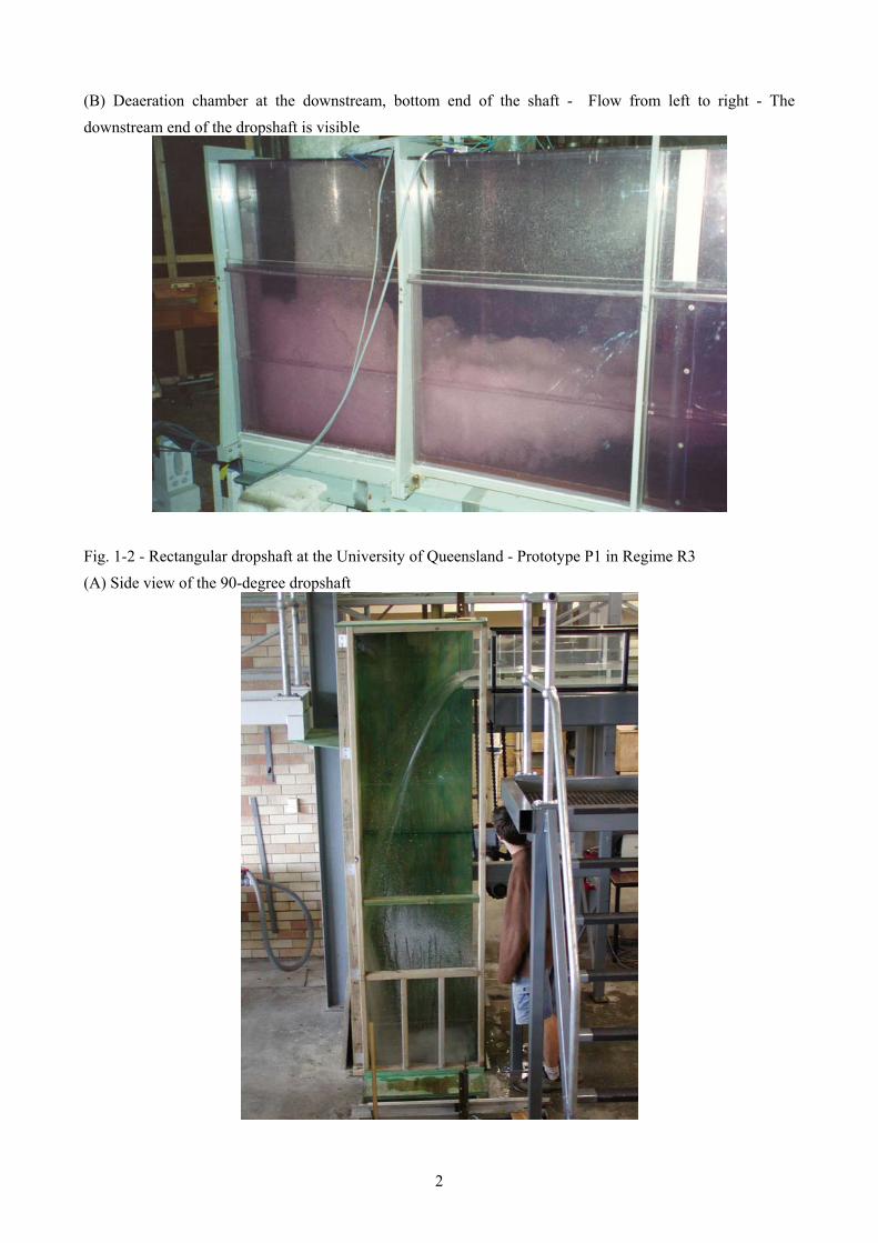
(B) Deaeration chamber at the downstream, bottom end of the shaft - Flow from left to right - The downstream end of the dropshaft is visible

Fig. 1-2 - Rectangular dropshaft at the University of Queensland - Prototype P1 in Regime R3 (A) Side view of the 90-degree dropshaft

3

(B) Looking into the shaft - At bottom end, the flow turns and exit to the right

Fig. 1-3 - Excavation of a dropshaft on the Yzeron Roman aqueduct (Lyon, France) : Puit Gouttenoire, Recret in November 2000 (Courtesy of Jean-Claude LITAUDON)

4

2. EXPERIMENTAL SETUP Five dropshaft geometries were studied basically in two flumes (Table 2-1, Fig. 2-1). Five models were built in marine plywood and perspex with a vertical rectangular shaft. The upstream channels were open while the downstream conduits were covered and ended with a free overfall. Both upstream and downstream channels were horizontal. For two geometries, two geometrically scaled shafts were built and tested : i.e., prototype P1 corresponding to Model 4, and prototype P2 corresponding to Model 5 (Table 2-1, Fig. 2-2). These configurations were designed to be geometrically similar based upon a Froude similitude with undistorted scale (e.g. HENDERSON 1966, CHANSON 1999). The geometric scaling ratio was LR = 3.1 in each case. Similar experiments were conducted for identical dimensionless inflow critical depth dc/h where dc is the critical depth at the brink and h is the invert drop in elevation. Measurements were performed at similar locations. Table 2-1 - Experimental investigations of rectangular dropshafts

Ref. h P L B l b1 D1 (1) b2 D2 Outflow direction

Remark

m m m m m m m m m deg. (1) (2) (3) (4) (5) (6) (7) (8) (9) (10) (11) (12)

Present 2.70 0 0.755 0.763 0.12 0.50 0.30 0.65 0.20 90 Prototype P1. study 1.70 1.00 0.755 0.763 0.12 0.50 0.30 0.50 0.30 180 Prototype P2. 0.87 0 0.243 0.246 0.039 0.161 0.25 0.209 0.064 90 Model 4. 0.548 0.322 0.243 0.246 0.039 0.161 0.25 0.209 0.097 180 Model 5. 0.548 0.322 0.243 0.246 0.039 0.161 0.25 0.209 0.097 90 Model 6. 0.548 0 0.243 0.246 0.039 0.161 0.25 0.209 0.097 180 Model 7. 0.548 0 0.243 0.246 0.039 0.161 0.25 0.209 0.097 90 Model 8. CHANSON 0.505 0.365 0.30 0.30 0 0.144 0.25 0.15 0.25 180 Recret model. (2002) 0.668 0.201 0.20 0.30 0 0.110 0.25 0.11 0.21 90 Valdepuentes

model 1. 0.668 0.201 0.20 0.30 0 0.110 0.25 0.11 0.21 180 Valdepuentes

model 2. APELT (1984)

0.325 0 0.152 0.152 0 Pipe : Ø = 0.152 m

Pipe : Ø = 0.152 m

180

Notes : (1) : sidewall height; Notation : see Figure 2-1.

Instrumentation In the smallest flume, the discharges were deduced from the brink depth measurements which were first calibrated in-situ with volume-per-time discharge data. A calibration curve was obtained for each model. In the largest dropshaft configurations, the flows rates were estimated from bend meters which were calibrated in-situ with a 90-degree V-notch weir. Free-surface elevations were recorded with pointer gauges in the upstream and downstream channels, while the free-surface height in the shaft was measured with rulers. The total head was measured with a total head tube (∅ = 1 mm). Measurements were conducted at 5 transverse profiles and averaged over the cross-section. [The averaging method was particularly important in the 90-degree bend dropshaft configurations and in the largest shafts.]

5

Fig. 2-1 - Definition sketch of rectangular dropshafts

Particle residence times were recorded using neutrally-buoyant particles (1) made of wax and aluminium. Several particle sizes were used : 3.3, 3.9, 5, 9 & 15 mm. The four smallest sizes were used in the models while the three largest sizes were used in the prototypes. The particles were introduced, one at a time, in the inflow channel about 1 m upstream of the brink and each particle was collected at the downstream end of the outflow channel, before the next particle was injected. The total travel times were recorded with digital chronometers. The residence time in the shaft was deduced by subtracting the calculated travel times in the inflow and outflow channels to the measured time. Air-water flow properties were measured with a single-tip conductivity probe (needle probe design). The probe consisted of a sharpened rod (platinum wire ∅ = 0.35 mm) which was insulated except for its tip and set into a metal supporting tube (stainless steel surgical needle ∅ = 1.42 mm) acting as the second electrode. The probe was excited by an electronics (Ref. AS25240) designed with a response time less than 10 µs and calibrated with a square wave generator. Further details on the probe design and electronic system were reported by CHANSON (1995) and CUMMINGS (1996). During the present study, the probe output signal

1Relative density between 0.95 and 1.05.

6

was scanned at 5 kHz for three minutes. Raw probe outputs were recorded at 20 kHz for 10 seconds to calculate bubble chord time distributions. Underwater acoustics were measured with a hydrophone (Dolphin Ear™) connected to a charge amplifier. The amplifier had a high-pass filter cut-off set at 400 Hz (2). The hydrophone was located at 20 mm beneath the free-surface and 20 mm away from the impingement perimeter for most experiments (3). Acoustic recordings were conducted for fifteen minutes. The signal was digitised with a SoundBlaster 16 card at 44.1 kHz, implying an alias frequency of about 22 kHz. The range of jet conditions caused a difference in acoustic signal power and the charge amplification range was selected for each experiment to deliver optimal recorded quality and corrected for during the signal processing. The data were processed by a bubble-acoustic software StreamTone™ (MANASSEH et al. 2001). Additional information were obtained with high-speed photography and video-camera.

Data processing The measurement principle of conductivity probes is based upon the difference in electrical resistivity between air and water. The resistance of water is one thousand times lower than the resistance of air bubbles. When the probe tip is in contact with water, current will flow between the tip and the supporting metal; when it is in contact with air no current will flow. Although the signal is theoretically rectangular, the probe response is not square because of the finite size of the tip, the wetting/drying time of the interface covering the tip and the response time of the probe and electronics. The air concentration, or void fraction C, is the proportion of time that the probe tip is in the air. Past experience showed that the probe orientation with the flow direction has little effect on the void fraction accuracy provided that the probe support does not affect the flow past the tip (e.g. SENE 1984, CHANSON 1988). In the present study, the probe tip was aligned with the flow direction. The bubble count rate F is the number of bubbles impacting the probe tip. The measurement is sensitive to the probe tip size, bubble sizes, velocity and discrimination technique, particularly when the sensor size is larger than the smallest bubble sizes. The bubble chord time is defined as the time spent by the bubble on the probe tip. Bubble chord times were calculated from the raw probe signal scanned at 20 kHz for 10 seconds at six different locations, per cross-section, selected next to the location of maximum void fraction and maximum bubble frequency. The signal was processed using a single threshold technique and the threshold was set at about 25% of the air-water voltage range. (An incomplete sensitivity analysis, conducted with thresholds between 10 and 35% of the voltage range, showed little effect of the threshold on chord time results. The results showed little effect of the threshold on chord time results.) The chord time results are presented in terms of pseudo-bubble chord length chab defined as : chab = Vi * tch (2-1)

2That is, it reached 100% at 400 Hz, admitting all frequencies above 400 Hz unchanged, and rolling off below 400 Hz. Hence acoustic data below 400 Hz can be disregarded. 3The hydrophone was attached to a hard-plastic support. The relative flexibility of the support ensured that its resonance frequency did not disturb the sound recordings.

7

where Vi is the jet impingement velocity and tch is the measured bubble chord time. CHANSON et al. (2002) compared Equation (2-1) with chord length measurements by CHANSON and BRATTBERG (1996) and CUMMINGS and CHANSON (1997b). The results showed that Equation (2-1) predicts the exact shape of bubble size probability distribution functions although it overestimates the bubble chord lengths by about 10 to 30%. The acoustic data were analysed following principles detailed in MANASSEH et al. (2001). A discrete, pulse-wise analysis was used. The technique can give good accuracy on the true bubble frequencies, but the conversion to bubble size spectra relies upon a questionable assumption that bubbles of different sizes are perturbed to the same proportional extent. It also assumes that the bubbles do not interact acoustically (CHANSON and MANASSEH 2003). The Streamtone™ software was set with a sound sampling rate of 11,025 Hz, a data length of 1000 samples, a trigger level of 0.1 Volt and a SuperWindow factor of 2.0 or 5.0. For four experiments (Q = 0.0076 and 0.016 m3/s, Regime R1; Q = 0.038 and 0.067 m3/s in Regime R3), the Streamtone™ software was also set with a sound sampling rate of 40,100 Hz, a data length of 1000 samples, a trigger level of 0.1 Volt and a SuperWindow factor of 20.0.

Experimental flow conditions The upstream and downstream channels operated as free-surface flow for all investigated flow conditions. All experiments were conducted with subcritical inflow conditions, while the outflow channel operated always with supercritical flows. CHANSON (2002) and RAJARATNAM et al. (1997) reported a similar finding. [Note that the outflow channels were relatively short and ended with a free overfall.]

8

Fig. 2-2 - Geometry of the prototype dropshafts (A) Prototype P1

9

(B) Prototype P2

10

3. FLOW PATTERNS

3.1 Presentation During the experiments, basic flow patterns were observed as functions of the flow rate and shaft configurations (Fig. 3-1 and 3-2). For a 180-degree shaft configuration with a deep pool (Fig. 3-1), the free-falling nappe impacted into the shaft pool at low flow rates (regime R1, Fig. 3-2A). Significant air was entrained at the jet impingement and large numbers of entrained air bubbles were observed in the shaft pool. For intermediate discharges, the jet flowed in between the inlet invert and obvert and the nappe impacted into the downstream channel invert (regime R2, Fig. 3-2B). Visually the rate of energy dissipation appeared smaller, and strong splashing and spray was seen in the downstream conduit associated with shock waves. The pool free-surface level increased significantly, and little air bubble entrainment was observed in the pool. At large flow rates, the free-jet impacted onto the opposite wall, above the downstream conduit obvert (regime R3, Fig. 3-2C and 3-2D). A vertical downward 'film' of water ran downwards along the wall, and the central section was deflected into the downstream conduit as a high velocity shooting flow. Significant water deflection took place in the shaft. Nappe impact onto the opposite wall was associated with the formation of a small roller described by RENNER (1973,1975) and RAJARATNAM et al. (1997). For the largest flow rate, the outflow channel inlet becomes submerged (Regime R3b, Fig. 3-2D). These observations were consistently noted in both model and prototype. They are consistent with the earlier study of CHANSON (1998,2002), although the downstream conduit was higher and the sub-regime R3b was not observed. For a 90-degree shaft configuration with a deep pool, the above observations were generally valid, but the regime R2 did not exist (CHANSON 2002). Only Regimes R1, R3a (free-surface outflow channel inlet) and R3b (submerged outflow channel inlet) were observed. In the models with no pool (i.e. P = 0), the above observations were basically valid, but air entrainment in the shaft pool was limited by the shaft invert (Fig. 1-2). However greater splashing was visually noticed in the shaft.

3.2 Transition between flow regimes In the present study, the transitions between regimes R1 and R2, and R2 and R3 were recorded and the results are presented in Tables 3-1 and 3-2. The experimental observations compared favourably with the analytical model of CHANSON (1998) (App. A). Table 3-1 - Flow conditions for the change in flow regimes - (1) 180 degree shaft configurations

Configuration Transition Remarks R1-R2 R2-R3a R3a-R3b

(1) (2) (3) (4) (5) Prototype P2 0.037 0.046 -- P = 1.0 m. Model 5 0.039 0.051 0.10 P = 0.32 m. Model 7 0.038 0.046 0.099 P = 0. Recret model 0.09 0.175 -- P = 0.36 m. CHANSON (2002). Valdepuentes model 2 0.029 0.042 -- P = 0.20 m. CHANSON (2002).

11

Table 3-2 - Flow conditions for the change in flow regimes - (2) 90 degree shaft configurations

Configuration Transition Remarks R1-R3a R3a-R3b

(1) (2) (3) (4) Prototype P1 0.013 -- P = 0. Model 4 0.017 0.060 P = 0. Model 6 0.037 0.12 P = 0.32 m. Model 8 0.035 0.11 P = 0. Valdepuentes model 2 0.028 -- P = 0.2 m. CHANSON (2002).

Fig. 3-1 - Definition sketch of rectangular dropshafts (180-degree configuration)

12

Figure 3-2 - Photographs of the various flow regimes (A) Regime R1 in Model 5 (h = 0.548 m, P = 0.322 m, 180-degree turn)

(B) Regime R2 in Prototype P2 (h = 1.7 m, P = 1.0, 180-degree turn)

13

(C) Regime R3a in Model 4 (h = 0.870 m, P = 0, 90-degree turn)

(D) Regime R3b in Model 4 (h = 0.870 m, P = 0, 90-degree turn)

14

4. HYDRAULIC PROPERTIES Basic hydraulic properties were recorded in the inflow and outflow channels, and in the shaft. The results are presented below. All experimental data are presented in Appendix B.

4.1 Dropshaft with deep shaft pool and 180 degree outflow direction Residual energy data are presented in Figure 4-1. The data are presented as H2/H1 as a function of the dimensionless flow rate dc/h where H2 is the residual head in the downstream channel, H1 is the upstream total head measured above the downstream channel invert, dc is the critical depth in the upstream channel and h is the drop in invert elevation. The results are compared with the data of CHANSON (2002). Low residual heads, associated with high energy dissipation, are achieved at low flow rates (Regime R1) (Fig. 4-1). Poor dissipation performances are observed in regime R2. In regime R3, the dimensionless residual head ranges from 20 to 35% depending upon the model geometry. Note the relatively good agreement between model and prototype data. Pool free-surface height data are reported in Figure 4-2 where yp is the free-surface height above downstream invert. Model and prototype data are close : they show an increase in pool height with increasing discharges. The results are consistent with the observations of RAJARATNAM et al. (1997), but differ from the data of APELT (1984) and CHANSON (2002). In the latter configurations, the outflow channel was taller and the obvert was not submerged. As a result, a slower increase in pool height with increasing flow rates was observed for Q' = Q/ g*b2*D3 > 0.4 (CHANSON 2002). The dimensionless bubble penetration depth is plotted in Figure 4-3 as a function of the dimensionless flow rate dc/h. In flow regimes R1 and R3, substantial flow aeration took place, the bubbles plunged deep down to the shaft pool and the bubble cloud occupied a sizeable shaft pool volume. The entrained bubbles enhance the air-water interface area and the air-water gas transfer : i.e., re-aeration. The flow regime R2 was less efficient in entraining air because the nappe interacted with the downstream conduit inlet. Interestingly, visual observations of bubble penetration depth showed smaller bubble swarm depths in the prototype. This visual result was consistent with air concentration measurements conducted in the shaft pool (section 6). It is likely that the result is related to some form of scale effects. Indeed air entrainment cannot be scaled by a Froude similitude (WOOD 1991, CHANSON 1997).

Discussion Compared with modern designs, the "Roman dropshaft" design exhibits an unusual shape : i.e., a deep wide shaft pool (CHANSON 1998,2000). Modern dropshafts do not include a pool, the shaft bottom being at the same elevation as the downstream channel bed to minimise construction costs. In Roman dropshafts, the pool of water acts as a cushion at nappe impact, preventing scour at the shaft bottom. The shaft pool facilitates further the entrainment (by plunging jet) of air bubbles deep down, maximising the bubble residence time and hence air-water mass transfer. The design contributes successfully to an enhancement of the DO content (dissolved oxygen content). Roman dropshafts had a wider shaft (i.e. B/b > 2) than modern designs (i.e. B/b = 1 to 1.5). It is believed that the wider shaft was selected for an easier construction and maintenance (e.g. BURDY 1996).

15

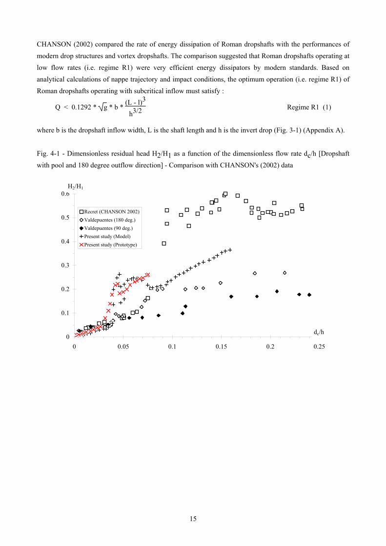
CHANSON (2002) compared the rate of energy dissipation of Roman dropshafts with the performances of modern drop structures and vortex dropshafts. The comparison suggested that Roman dropshafts operating at low flow rates (i.e. regime R1) were very efficient energy dissipators by modern standards. Based on analytical calculations of nappe trajectory and impact conditions, the optimum operation (i.e. regime R1) of Roman dropshafts operating with subcritical inflow must satisfy :

Q < 0.1292 * g * b * (L - l)3

h3/2 Regime R1 (1)

where b is the dropshaft inflow width, L is the shaft length and h is the invert drop (Fig. 3-1) (Appendix A). Fig. 4-1 - Dimensionless residual head H2/H1 as a function of the dimensionless flow rate dc/h [Dropshaft with pool and 180 degree outflow direction] - Comparison with CHANSON's (2002) data

0

0.1

0.2

0.3

0.4

0.5

0.6

0 0.05 0.1 0.15 0.2 0.25

Recret (CHANSON 2002)Valdepuentes (180 deg.)Valdepuentes (90 deg.)Present study (Model)Present study (Prototype)

dc/h

H2/H1

16

Fig. 4-2 - Dimensionless pool height yp/D as a function of the dimensionless flow rate Q' = Q/ g*b2*D3 [Dropshaft with pool and 180 degree outflow direction] - Comparison with the data of APELT (1984), RAJARATNAM et al. (1997) and CHANSON (2002)

0

0.2

0.4

0.6

0.8

1

1.2

1.4

1.6

1.8

0 0.2 0.4 0.6 0.8 1

APELT B/D=1APELT B/D=1.3RAJARATNAMRecret (CHANSON 2002)Valdepuentes (180 deg.)Valdepuentes (90 deg.)Present study (model)Present study (Prototype)

Q'

yp/D

Fig. 4-3 - Dimensionless bubble penetration depth Dab/(yp+h) as a function of the dimensionless flow rate dc/h [Dropshaft with pool and 180 degree outflow direction] - Comparison with CHANSON's (2002) data

0

0.2

0.4

0.6

0.8

1

0 0.05 0.1 0.15 0.2 0.25

Recret (CHANSON 2002)Valdepuentes (180 deg.)Valdepuentes (90 deg.)Present study (Model)Present study (Prototype)

dc/h

Dab/(yp+P)

Regime R2 (Recret)

Regime R2 (Valdepuentes 180 deg)

Regime R2 (Present study)

17

4.2 Effects of pool depth and outflow direction The effects of pool depth and outflow direction were systematically investigated for two shaft pool depths (P = 0 & 0.32 m) and two outflow directions (90º & 180º) in models, all other dropshaft parameters being kept constant. That is, with Model 5 (P = 0.32 m, 180º), Model 6 (P = 0.32 m, 90º), Model 7 (P = 0, 180º) and Model 8 (P = 0, 90º). All other shaft characteristics were identical (Table 2-1). Figures 4-4 and 4-5 present some comparative results. The full data set is presented in Appendix B. Comparative results showed that the absence of pool had little effect on the residual energy (Fig. 4-4). But greater rate of energy dissipation was observed with the 90º outflow direction (all other parameters being identical). The result is illustrated in Figure 4-4, where the dimensionless residual head in Models 6 and 8 (90º outflow direction) are consistently smaller than those in Models 5 and 7, especially in regimes R2 and R3. The findings agree with the study of CHANSON (2002) on the Valdepuentes dropshaft models. The pool depth and outflow direction had little effects on the water depth in the shaft pool (Fig. 4-5), while the outflow direction had little impact on the bubble penetration depth, but in flow regime R2. Fig. 4-4 - Dimensionless residual head H2/H1 as a function of the dimensionless flow rate dc/h - Model studies with P = 0 & 0.32 m, and 90-degree and 180-degree outflow directions

0

0.1

0.2

0.3

0.4

0 0.05 0.1 0.15

Model 5 P=0.32m, 180 degModel 6 P=0.32m, 90 degModel 7 P=0, 180 degModel 8 P=0, 90 deg

dc/h

H2/H1Model studies (h = 0.55 m)

18

Fig. 4-5 - Dimensionless pool height yp/D as a function of the dimensionless flow rate Q' = Q/ g*b2*D3 - Model studies with P = 0 & 0.32 m, and 90-degree and 180-degree outflow directions

0

0.5

1

1.5

2

0 0.1 0.2 0.3 0.4 0.5 0.6

Model 5 P=0.32m, 180 degModel 6 P=0.32m, 90 degModel 7 P=0, 180 degModel 8 P=0, 90 deg

Q'

yp/DModel studies (h = 0.55 m

19

5. PARTICLE RESIDENCE TIMES

5.1 Introduction The residence times of neutrally-buoyant particles were measured in the shaft. The shaft residence time is defined from take-off at the brink of the inflow channel to the entry into the outflow channel. Experiments were repeated with three to four particle sizes for each configuration and flow rate, and for at least 40 to 50 times with each particle size. A summary of the data is presented in Table 5-1. Experimental data are presented in Appendix C. First the results showed that the data were basically independent of the particle sizes (3.3 to 9 mm in model, 5 to 15 mm in prototype) for all flow regimes and configurations. Thereafter the data are regrouped for all particle sizes. Second, for one dropshaft configuration and one flow regime, the probability distribution functions of dimensionless residence time T*Vc/dc were basically independent of the flow rate, where dc is the critical depth at the inflow channel brink and Vc is the corresponding critical velocity. In turn, the data for one geometry and one flow regime (1) were collated together. The particle residence times provide some information on the water particle transit times. A related study was conducted by ELATA and IPPEN (1961), although their focus was on the interactions between neutrally-buoyant spherical particles and turbulence.

5.2 Basic results Typical probability distribution functions of dimensionless residence times are presented in Fig. 5-1 for two dropshaft configurations with deep pools and 180-degree angle between inflow and outflow channel directions. Both data sets exhibit similar trend. A third data set is presented for an identical model configuration but with a 90-degree outflow direction (Fig. 5-1C).

5.2.1 Dropshaft with deep pool and 180 deg. outflow direction In regime R1, the dimensionless particle residence time was comparatively the greatest, corresponding to the entrainment of particles in the shaft pool and, sometimes, their trapping in large-size vortical structures for a significant duration. In the regime R2, the free-falling nappe flowed directly into the outflow channel. Most particles were directly entrained into the outflow conduit, corresponding to a very-small residence time. The residence time was about the free-jet trajectory time. In the regime R3, particles were sometimes entrained down the shaft pool but most exited the shaft rapidly. The same trends were observed in both model and prototype, and they are emphasised by mean particle residence time results (Table 5-1, column 5). Figure 5-2 presents a comparison between model and prototype data, for a dropshaft geometry with deep pools and 180-degree between inflow and outflow channel directions. Figures 5-2A, 5-2B and 5-2C regroups respectively regime R1, R2 and R3 data. In regime R1, the residence time probability distributions exhibit a bi-modal shape. For the data shown in Figure 5-2A, the Mode 1 is centered around T*Vc/dc = 66 and 33 for model and prototype respectively, while Mode 2 is centered roughly around T*Vc/dc = 1770 and 1230 for model and prototype (Table 5-1, columns 11 and 12). These values may be compared with the average filling

1Typically for the flow regimes R1 and R3.

20

time of the shaft pool of about T*Vc/dc = 770 (Table 5-1, column 13). Physically, about 40-50% of the particles flowed downwards at nappe impact and were entrained rapidly into the outflow channel (Mode 1). The rest of particles (i.e. 50-60%) were trapped in large scale vortices (Mode 2). They were seen to recirculate in large-scale flow structures, sometimes passing from one structure to another, until they were finally entrained in the downstream conduit. In average, such Mode 2 particles stayed in the shaft pool for about 2.5 times the average filling time of the shaft pool. In regime R3, dimensionless particle residence time data suggest also a kind of bimodal distribution, although not as marked as in regime R1. The results are illustrated in Figure 5-2C and summarised in Table 5-1 (columns 11 and 12). About 65-70% of the particles exited rapidly from the shaft, while about 30-35% of the particles were trapped in recirculation vortices (Mode 2) for, in average, about 4 to 6 times the average filling time of the shaft pool. Fig. 5-1 - Probability distribution functions of dimensionless residence time T*Vc/dc for several dropshaft geometries (A) Model 5 (180 deg. outflow)

��

��

��

��

��

��

0

0.1

0.2

0.3

0.4

0.5

0 30 60 90 120

150

180

210

240

270

300

330

>360

Regime R1 (253 particles)Regime R2 (99 particles)��

�� Regime R3 (180 particles)

Model M5 - Drophaft with deep pool (180 deg.)

T*Vc/dc

(B) Prototype P2 (180 deg. outflow)

��

��

��

0

0.1

0.2

0.3

0.4

0.5

0 30 60 90 120

150

180

210

240

270

300

330

>360

Regime R1 (380 particles)Regime R2 (86 particles)��

�� Regime R3 (227 particles)

Prototype P2 - Drophaft with deep pool (180 deg.)

T*Vc/dc

0.71

21

(C) Model 6 (90 deg. outflow)

��

��

��

��

��

��

��

��

��

��

��

��

��

��

��

0

0.1

0.2

0.30 30 60 90 120

150

180

210

240

270

300

330

>360

Regime R1 (189 particles)�� Regime R3 (292 particles)

Model M6 - Drophaft with deep pool (90 deg.)

T*Vc/dc

Pdf

5.2.2 Dropshaft with deep pool and 90 deg. outflow direction In dropshafts with 90-degree outflow direction and deep pool, particles had to be subjected to change in flow direction before exiting. Visually, most particles tended to be entrained deep down the pool shaft, to turn around near the shaft bottom and to flow outwards rapidly. The same pattern was observed in both regimes R1 and R3. Figure 5-3 compares the dimensionless particle times for two identical model dropshafts, but for the outflow direction, in regimes R1 and R3. In average the particle residence times were smaller than in the 180-degree outflow direction configuration, all other parameters being identical (Table 5-1, column 5). Figure 5-3 shows further a higher proportion of particles with very large residence times (T*Vc/dc > 500) in the 180 deg. dropshaft configuration. Table 5-1 - Distributions of dimensionless particle residence times T*Vc/dc - Statistical summary Config. Regim. Particle

∅ Nb of

particle T * Vc

dc

T * Vcdc

Vol*Vc

Q*dc

(mm) Mean Std Skew Kurt Min. Max. 1st Mode

2nd Mode

Shaft pool

(1) (2) (3) (4) (5) (6) (7) (8) (9) (10) (11) (12) (13) Model M5 R1 3.9, 5 253 1050 1635 2.66 8.08 15 9580 66 1771 765 (180 deg.) R2 3.3, 5 99 80 170 3.66 14.86 5 986 10 N/A 229 R3 3.3, 5 180 246 519 4.76 32.34 6 4706 18 490 124 Prototype P2 R1 5, 9, 15 380 830 1150 1.87 3.22 13 5787 33 1230 769 (180 deg.) R2 9.15 86 188 503 3.56 13.28 5 2728 6 N/A 228 R3 5, 9, 15 227 209 459 2.72 7.17 6 2543 14 750 127 Model M6 R1 3.5, 5 189 653 1119 3.06 12.02 27 7282 79 1272 829 (90 deg.) R3 3.5, 5 292 111 117 5.46 46.62 14 1349 79 311 129

Notes : Kurt : Fisher kurtosis; Skew : Fisher skewness; Vol : shaft pool volume; Q : flow rate.

22

5.3 Discussion In Regime R1, the large particle residence times implied a strong mixing between the inflow and the shaft pool waters. In turn, entrained air bubbles stayed longer underwater and contributed more significantly to mass transfer. Dropshaft are indeed well-known aeration devices. Fig. 5-2 - Probability distribution functions of dimensionless residence time T*Vc/dc : comparison between model and prototype data (model 5, prototype P2) for 180 deg. outflow direction (A) Regime R1

0

0.1

0.2

0.3

0 50 100

150

200

250

300

350

400

450

500

550

600

650

700

750

800

850

900

950

>100

0

Model 5 (253 particles)Prototype P2 (380 particles)

Regime R1 - Drophaft with deep pool (180 deg.)

T*Vc/dc

0.34

(B) Regime R2

0

0.1

0.2

0.3

0.4

0 10 20 30 40 50 60 70 80 90 100

110

120

130

140

150

160

170

180

190

>200



T*Vc/dc

23

In Figure 5-2, all the data suggest a similar trend in model and prototype, although prototype results suggest smaller dimensionless residence times for all flow regimes. Such observations of scale effects between model and prototype (Fig. 5-2) imply that model data would tend to overestimate residence times, hence mass transfer rates, based upon a Froude similitude. It is believed that particle residence times is strongly related to vortical motion in the shaft pool which cannot be scaled by a Froude similitude. In turn, the results highlight some scale effects between the two geometries. Interestingly, regime R3 results suggest that the average, dimensionless residence times of particles trapped in recirculation regions (Mode 2) were larger in prototype that in model. No explanation is yet available. Fig. 5-2 (C) Regime R3

0

0.1

0.2

0.3

0.4

0.5

0.6

0.7

0 25 50 75 100

125

150

175

200

225

250

275

300

325

350

375

400

425

450

475

>500



T*Vc/dc

Fig. 5-3 - Probability distribution functions of dimensionless residence time T*Vc/dc : effect of outflow direction - Comparison between models M5 (180 deg.) and M6 (90 deg.) (A) Regime R1

0

0.1

0.2

0 50 100

150

200

250

300

350

400

450

500

550

600

650

700

750

800

850

900

950

>100

0

Model 5 (253 particles)Model 6 [90 deg.] (189 particles)

Regime R1 - Model drophaft with deep pool (180 & 90 deg.)

T*Vc/dc

0.34Pdf

24

(B) Regime R3

0

0.1

0.2

0.3

0.40 25 50 75 100

125

150

175

200

225

250

275

300

325

350

375

400

425

450

475

>500

Model 5 (180 particles)Model 6 [90 deg.] (292 particles)

Regime R3 - Model drophaft with deep pool (180 & 90 deg.)

T*Vc/dc

Pdf

25

6. AIR-WATER FLOW PROPERTIES

6.1 Introduction Strong aeration was observed in the shaft pool for the "Roman dropshaft" configuration (i.e. P > 0). Detailed air-water flow measurements were conducted with a sturdy single-tip conductivity probe in the prototype P2 (Fig. 6-1). Experimental data are presented in Appendices D and E. A summary of the investigated flow conditions is presented in Table 6-1. Time-averaged data (i.e. void fraction and bubble count rate) are presented in section 6.2, while microscopic observations (i.e. bubble chord times) are presented in section 6.3. Preliminary measurements conducted at various transverse locations y indicated that the void fraction distributions were basically two-dimensional, but next to the outside edges of the free-falling nappe impact. In turn, measurements were conducted next to the jet centreline to characterise the two-dimensional flow region while two additional profiles were performed next to the jet outside edges (Table 6-1, column 5). Table 6-1 - Summary of air-water flow measurements in dropshaft prototype P2

Q Flow regime

db (1) yp (1) y z xi (1),

(2)

yi (1) Vi (2) di (2) Remarks

m3/s m m m m m m/s m (1) (2) (3) (4) (5) (6) (7) (8) (9) (10) (11)

0.0076 R1 0.0203 0.015 0 0.03, 0.05, 0.08, 0.11, 0.15, 0.20

0.223-0.228

0.17 5.81 0.0026 Prototype P2 (L = 0.755 m). dc = 0.02867 m.

0.20 0.08, 0.11, 0.15, 0.20

0.22 0.15, 0.20 0.016 R1 0.034 0.080 0 0.03, 0.05,

0.08, 0.15, 0.25, 0.35

0.098-0.106

0.23 5.74 0.0056 Prototype P2 (L = 0.755 m). dc = 0.0471 m.

0.20 0.03, 0.08, 0.15, 0.25,

0.35

0.25 0.08, 0.15, 0.25, 0.35

0.067 R3 0.091 0.266 0 0.03, 0.05, 0.08, 0.15, 0.25, 0.35

N/A 0.25 full

width

5.58 N/A Prototype P2 (L = 0.755 m). dc = 0.12237 m.

0.20 0.03, 0.05, 0.08, 0.15, 0.25, 0.35

0.30 0.03, 0.05, 0.08, 0.15, 0.25, 0.35

Notes : xi, yi : nappe impact location; Vi, di : jet impact velocity and thickness deduced from trajectory equations; (1) : measured; (2) : calculated (Appendix A).

26

Figure 6-1 - Dropshaft Prototype P2 in operation with the single-tip conductivity probe for Q = 16 L/s

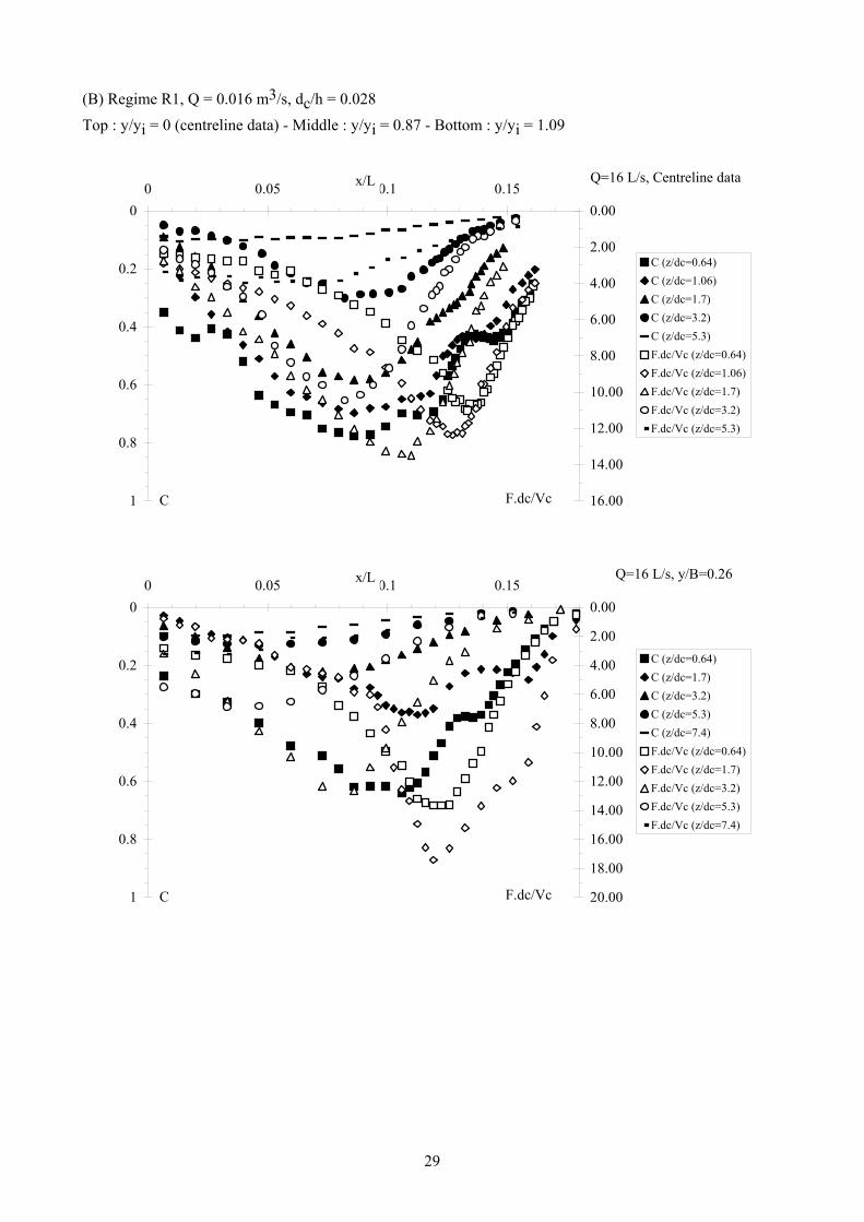
6.2 Void fraction and bubble count rates Typical distributions of void fraction C and dimensionless bubble count rate F*dc/Vc are presented in Figure 6-2, where F is the bubble count rate (2), dc and Vc are the critical depth and velocity respectively at the inflow channel brink, x is the horizontal distance measured from the downstream shaft wall, z is the vertical direction positive downwards with z = 0 at the pool free-surface and y is the horizontal transverse distance from the shaft centreline (Fig. 2-1). The full data set is presented in Appendix D. All experimental profiles traversed the full length of the shaft. Absence of data indicates void fractions less than 0.5%. Figures 6-2A, 6-2B and 6-2C present experimental data for dc/h = 0.017, 0.028 and 0.072 respectively at several vertical locations z/dc. Experimental results demonstrated very high void fractions next to the free-surface for all three flow conditions : that is, for z < 50 mm (Fig. 6-2). Large measured void fractions could not be attributed to measurement error (3). However, the plunge point region was visually very aerated and it had an appearance

2That is, the number of bubbles detected by the probe sensor per second. 3Measurements were repeated independently by two research students and the writer. The results showed no measurement discrepancy between experimentator.

27

somehow similar to a hydraulic jump roller. Further the pool free-surface elevation fluctuated at low frequency with time (4). It is conceivable that the probe tip was in air for brief periods, although this was not visually observed. Void fraction distributions showed that the measurements were performed in the fully-developed flow region : i.e., 10 ≤ z/di ≤ 70 typically where di is the jet thickness at impact. For comparison, the classical experiments of CUMMINGS and CHANSON (1997a,b) and BRATTBERG and CHANSON (1998) were conducted in the developing flow region corresponding to z/di < 10. Distributions of bubble count rates exhibit a marked peak (Fig. 6-2). For a given flow rate, the longitudinal distributions of maximum count rate do not present the longitudinal decay in maximum void fraction (Table 6-2, columns 6 and 7). Observed values of maximum bubble count rates ranged from 20 to 200 Hz, that are consistent with experiments by CHANSON and TOOMBES (2002a,b) in stepped chutes using the same single-tip conductivity probe system. Figure 6-2 - Dimensionless distributions of void fraction C and bubble count rate F*dc/Vc in the shaft pool (A) Regime R1, Q = 0.0076 m3/s, dc/h = 0.017 Top : y/yi = 0 (centreline data) - Middle : y/yi = 1.18 - Bottom : y/yi = 1.29

0

0.2

0.4

0.6

0.8

1

0.2 0.25 0.3 0.350.00

2.00

4.00

6.00

8.00

10.00

12.00

C (z/dc=1.05)C (z/dc=1.74)C (z/dc=2.8)C (z/dc=3.8)C (z/dc=5.2)F.dc/Vc (z/dc=1.05)F.dc/Vc (z/dc=1.74)F.dc/Vc (z/dc=2.8)F.dc/Vc (z/dc=3.8)F.dc/Vc (z/dc=5.2)

x/L

C F.dc/Vc

Q=7.6 L/s, Centreline data

4The natural sloshing period of shaft pool was about 0.5 s.

28

0

0.2

0.4

0.6

0.8

1

0.2 0.25 0.3 0.350.00

2.00

4.00

6.00

8.00

10.00

12.00

C (z/dc=2.8)C (z/dc=3.8)C (z/dc=5.2)C (z/dc=7.0)F.dc/Vc (z/dc=2.8)F.dc/Vc (z/dc=3.8)F.dc/Vc (z/dc=5.2)F.dc/Vc (z/dc=7.0)

x/L

C F.dc/Vc

Q=7.6 L/s, y=200 mm

0

0.2

0.4

0.6

0.8

1

0.2 0.25 0.3 0.350.00

2.00

4.00

6.00

C (z/dc=5.2)C (z/dc=7.0)F.dc/Vc (z/dc=5.2)F.dc/Vc (z/dc=7.0)

x/L

C F.dc/Vc

Q=7.6 L/s, y=220 mm

29

(B) Regime R1, Q = 0.016 m3/s, dc/h = 0.028 Top : y/yi = 0 (centreline data) - Middle : y/yi = 0.87 - Bottom : y/yi = 1.09

0

0.2

0.4

0.6

0.8

1

0 0.05 0.1 0.150.00

2.00

4.00

6.00

8.00

10.00

12.00

14.00

16.00


x/L

C F.dc/Vc

Q=16 L/s, Centreline data

0

0.2

0.4

0.6

0.8

1

0 0.05 0.1 0.150.00

2.00

4.00

6.00

8.00

10.00

12.00

14.00

16.00

18.00

20.00


x/L

C F.dc/Vc

Q=16 L/s, y/B=0.26

30

0

0.2

0.4

0.6

0 0.05 0.1 0.150.00

2.00

4.00

C (z/dc=1.7)C (z/dc=3.2)C (z/dc=5.3)C (z/dc=7.4)F.dc/Vc (z/dc=1.7)F.dc/Vc (z/dc=3.2)F.dc/Vc (z/dc=5.3)F.dc/Vc (z/dc=7.4)

x/L

C F.dc/Vc

Q=16 L/s, y/B=0.33

(C) Regime R3a, Q = 0.067 m3/s, dc/h = 0.072 Top : y/yi = 0 (centreline data) - Middle : y/yi = 0.80 (?) - Bottom : y/yi = 1.2 (?)

0

0.2

0.4

0.6

0.8

1

0 0.05 0.10.00

2.00

4.00

6.00

8.00

10.00

12.00

14.00

16.00

18.00

20.00

22.00

24.00


x/L

C F.dc/Vc


31

0

0.2

0.4

0.6

0.8

1

0 0.05 0.10.00

2.00

4.00

6.00

8.00

10.00

12.00

14.00

16.00

18.00

20.00

22.00

24.00


x/L

C F.dc/Vc

Q=67 L/s, y=200 mm

0

0.2

0.4

0.6

0.8

1

0 0.05 0.10.00

2.00

4.00

6.00

8.00

10.00

12.00

14.00

16.00

18.00

20.00

22.00

24.00


x/L

C F.dc/Vc

Q=67 L/s, y=300 mm

Discussion In regime R1, the plunging jet flow is characterised by smooth, derivative profiles of void fractions (Fig. 6-2). In each experiment, the centreline data illustrated consistently the advective diffusion of entrained air associated with a quasi-exponential decay of maximum air content with longitudinal distance from impingement and a broadening of the air diffusion layer. The data were best fitted by an analytical solution of the diffusion equation for air bubbles :

32

C = 12

QairQ

1

8 π D# zdi

exp

- 1

2 D#

x - xi

di -

12

2

zdi

+ exp

- 1

2 D#

x - xi

di +

12

2

zdi

Two-dimensional free-falling plunging jet (6-1)

where Qair is the volume air flow rate, Q is the water discharge, di is the thickness of the free-jet at impact and xi is the jet impact coordinate (CUMMINGS and CHANSON 1997a) (5). D# is a dimensionless diffusivity : D# = Dt/(Vi di). Equation (6-1) is shown in Figure 6-3. The values of D# and Qair/Q were

determined from the best fit of the data and they are given in Table 6-2 (columns 8 & 9). Table 6-2 - Analysis of void fraction distributions in dropshaft prototype P2

Q Flow regime

Vi (1) y z/di Cmax Fmax QairQ (2) D# (2) Remarks

m3/s m/s m Hz (1) (2) (3) (4) (5) (6) (7) (8) (9) (10)

0.0076 R1 5.81 0 11 0.57 154.4 24 6 Centreline 19 0.51 193.3 21.5 3.5 data. 31 0.39 159.1 16.5 2.4 42 0.38 154.2 20 2.8 57 0.14 69.8 8 2.2 76 0.04 21.2 2.3 1.6

0.016 R1 5.74 0 5 0.77 158.9 31 12 Centreline 9 0.70 178.5 23 4.7 data. 14 0.58 194.3 15.5 1.9 27 0.30 150.7 6.9 0.85 45 0.10 57.0 -- -- 63 0.05 21.0 -- --

0.067 R3a 5.58 0 1.2 0.67 151.1 N/A N/A Centreline 2.1 0.59 165.6 data. 3.3 0.42 195.9 6.2 0.17 165.0 10.4 0.09 55.8 14.6 0.10 62.2

Notes : (1) calculated from nappe trajectory equations; (2) : values determined from best fit of data.

5Note a notation error in the original Equation (8a) in CUMMINGS and CHANSON (1997a) where d1 should be the half-jet thickness.

33

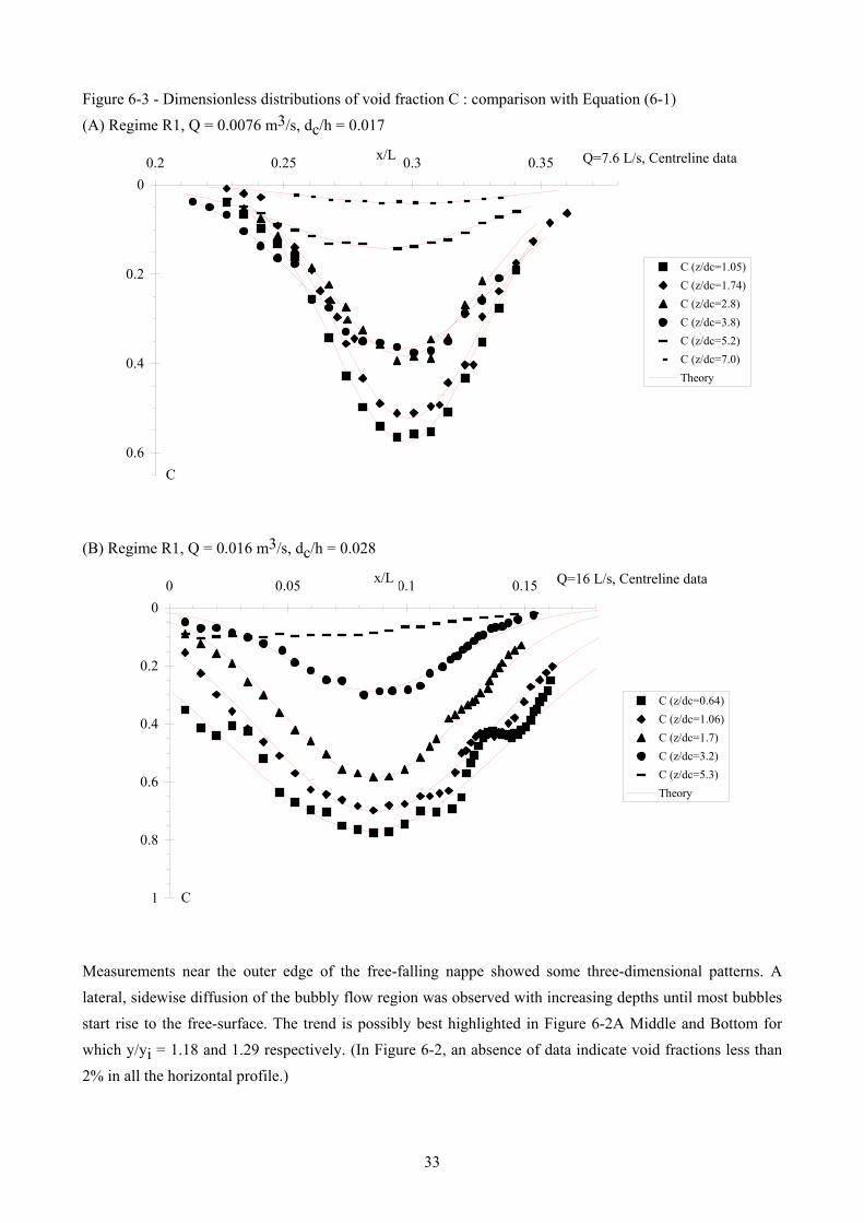
Figure 6-3 - Dimensionless distributions of void fraction C : comparison with Equation (6-1) (A) Regime R1, Q = 0.0076 m3/s, dc/h = 0.017

0

0.2

0.4

0.6

0.2 0.25 0.3 0.35

C (z/dc=1.05)C (z/dc=1.74)C (z/dc=2.8)C (z/dc=3.8)C (z/dc=5.2)C (z/dc=7.0)Theory

x/L

C

Q=7.6 L/s, Centreline data

(B) Regime R1, Q = 0.016 m3/s, dc/h = 0.028

0

0.2

0.4

0.6

0.8

1

0 0.05 0.1 0.15

C (z/dc=0.64)C (z/dc=1.06)C (z/dc=1.7)C (z/dc=3.2)C (z/dc=5.3)Theory

x/L

C


Measurements near the outer edge of the free-falling nappe showed some three-dimensional patterns. A lateral, sidewise diffusion of the bubbly flow region was observed with increasing depths until most bubbles start rise to the free-surface. The trend is possibly best highlighted in Figure 6-2A Middle and Bottom for which y/yi = 1.18 and 1.29 respectively. (In Figure 6-2, an absence of data indicate void fractions less than 2% in all the horizontal profile.)

34

When the free-falling nappe impacted in the shaft pool (i.e. regime R1), the lateral diffusion of entrained air bubbles near the outer edge of the nappe (y > yi) followed somehow an analytical solution of the air bubble advective diffusion equation for circular plunging jets :

C = Q'air

Q' * 1

8 * D* * zdi

* exp

- 1

8 * D* *

r

di / 22

+ 1

zdi

* Io

1

2 * D* *

rdizdi

(6-2)

where Q'air/Q' is the rate of air entrainment near the outer edge of the nappe, D* = 2*D't/(V1*di) is a

dimensionless air bubble diffusivity, and r is the radial distance with r = 0 at x = xi and y = (yi - di/2) :

r = (x - xi)2 +

y -

yi - di2

2 for y > yi

6.3 Bubble chord time distributions The bubble chord time tch is defined as the time spent by a bubble on the probe sensor. Chord time data were calculated from the raw signal scanned at 20 kHz at 6 locations per cross-section. The results are presented in terms of pseudo-bubble chord length chab defined as : chab = Vi * tch (2-1)

where Vi is the jet impingement velocity and tch is the measured bubble chord time. Equation (2-1) predicts accurately the shape of chord size probability distribution functions although it overestimates bubble chord lengths by about 10 to 30% (CHANSON et al. 2002).

Observations of pseudo-bubble chord sizes Pseudo-bubble chord length distribution results are shown in Figure 6-4 and the complete data set is reported in Appendix E. In Figure 6-4, each figure shows the normalised probability distribution function of pseudo-chord length chab where the histogram columns represent the probability of chord length in 0.5 mm intervals : e.g., the probability of a chord length from 2.0 to 2.5 mm is represented by the column labelled 2.0. The last column (i.e. > 15) indicates the probability of chord lengths exceeding 15 mm. Each histogram describes the bubbles detected in a cross-section (i.e. 6 locations) at depths z = 30, 50, 80, 150 and 250 mm. Statistical properties of the pseudo-chord size distributions are summarised in Table 6-3. Means, standard deviations, skewness and kurtosis of pseudo-bubble chord sizes are given in columns 5 to 8. The results highlight that the mean pseudo-bubble chord sizes were typically between 10 and 20 mm. Columns 9 to 12 (Table 6-3) list the means, standard deviations, skewness and kurtosis of pseudo-water chord sizes. These provide additional information on the streamwise distribution of air bubbles. For all flow conditions, the data demonstrated the broad spectrum of pseudo-bubble chord lengths at each cross-section : i.e., from less than 0.5 mm to larger than 25 mm (Fig. 6-4). The pseudo-bubble chord length distributions were skewed with a preponderance of small bubble sizes relative to the mean. The probability of bubble chord length was the largest for bubble sizes between 0 and 2 mm although the mean pseudo-chord size was much larger (Table 6-3). The trends were emphasised by positive skewness and large kurtosis (Table 6-3, columns 7 and 8). It is worth noting the large fraction of bubbles larger than 15 mm next to the

35

free-surface : that is, for z = 30 mm (Fig. 6-4). These large bubbles may be large air packets entrapped at impingement which were subsequently broken up by turbulent shear. Basically the results highlighted that the mean pseudo-chord sizes were between 10 and 20 mm. That is, there was a predominance of large entrained air packets for all flow conditions. The trend was consistent with experimental measurements in the developing flow region of vertical plunging jets (CUMMINGS and CHANSON 1997b, CHANSON et al. 2002). Further there was a large fraction of bubbles larger than 15 mm next to the impingement perimeter (i.e. z = 30 mm, Fig. 6-4) and the mean pseudo-bubble chord sizes decreased with increasing distance z from the free-surface for a given flow conditions (Table 6-3, column 5). The result implies the entrainment of large air packets which are subsequently broken up by turbulent shear. The trend was similar for all three flow conditions suggesting a similar bubble breakup process. Table 6-3 - Statistical properties of pseudo chord length distributions (centreline data)

Q z x Nb Air chord Water chord bubble Mean Std Skew Kurt Mean Std Skew Kurt

L/s mm mm mm mm mm mm (1) (2) (3) (4) (5) (6) (7) (8) (9) (10) (11) (12) 7.6 30 215-240 7650 28.2 54.5 3.6 16.7 14.9 29.0 6.0 57.2

50 216-241 10500 20.8 39.4 3.7 19.0 12.9 26.7 8.8 173.0 80 216-241 7650 15.2 29.0 4.2 23.6 13.9 27.6 13.7 483.8 110 207-232 10157 13.3 24.8 5.2 49.8 21.3 43.2 5.6 44.9 150 207-232 7896 11.9 21.8 6.1 68.5 33.0 77.1 7.4 84.8 200 207-232 3014 10.7 16.2 3.8 21.8 100.8 313.6 7.1 68.2

16 30 103-118 7369 19.9 35.1 3.7 17.3 26.5 46.8 4.6 31.8 50 98-113 7868 17.8 32.2 4.0 21.0 24.5 45.3 5.0 36.8 80 62-77 11597 23.0 45.8 3.8 18.5 7.0 12.4 6.8 100.4 150 61-76 8031 12.8 23.6 4.6 29.8 23.7 63.5 10.3 161.3 250 04-19 7287 12.1 16.7 5.6 63.1 35.9 66.1 5.7 50.6 350 25-40 3965 15.4 18.0 3.5 20.1 68.6 160.9 8.3 93.7

67 30 16-31 8199 25.4 44.0 3.6 18.9 17.3 29.1 4.8 38.8 50 16-31 9456 16.5 28.4 3.6 17.4 16.2 27.9 5.1 45.7 150 04-19 10165 7.7 12.8 4.4 23.7 22.6 41.8 4.8 38.2 250 04-19 6855 7.9 15.9 5.4 45.0 27.9 57.9 4.1 24.3 350 10-25 6074 10.2 17.4 5.3 41.9 50.2 93.3 4.5 29.8

Notes : Skew : Fisher skewness; Kurt : Fisher kurtosis; Bold underlined : suspicious data.

36

Fig. 6-4 - Pseudo-bubble chord length distributions (chab = Vi * tch) in Prototype P2 (centreline data) (A) Q = 0.0076 m3/s, Regime R1

��

��

��

��

��

��

��

��

��

��

��

��

��

��

��

��

��

��

��

��

��

��

��

��

��

��

��

��

��

��

0

0.1

0 1 2 3 4 5 6 7 8 9 10 11 12 13 14 >15

Z=30 mmZ=80 mm��

�� Z=150 mm

Vi * tch ( )

Pdf Q=7.6 L/s 0.230.35 0.2

(B) Q = 0.016 m3/s, Regime R1

��

��

��

��

��

��

��

��

��

��

��

��

��

��

��

��

��

��

��

��

��

��

��

��

��

��

��

��

��

��

��0

0.1

0 1 2 3 4 5 6 7 8 9 10 11 12 13 14 >15

Z=30 mm�� Z=150 mm

Z=250 mm

Vi * tch ( )

Pdf Q=16 L/s 0.30.3 0.2

(C) Q = 0.067 m3/s, Regime R3a

��

��

��

��

��

��

��

��

��

��

��

��

��

��

��

��

��

��

��

��

��

��

��

��

��

��

��

��

0

0.1

0 1 2 3 4 5 6 7 8 9 10 11 12 13 14 >15

Z=30 mmZ=150 mm

��Z=250 mm

Vi * tch ( )

Pdf Q=67 L/s 0.140.370.2

0.1

37

Fig. 6-5 - Pseudo-water chord length distributions (chw = Vi * tch) in Prototype P2 (centreline data) (A) Q = 0.0076 m3/s, Regime R1

��

��

��

0

0.1

0.2

0 1 2 3 4 5 6 7 8 9 10 11 12 13 14 >15

Z=80 mmZ=150 mm��

�� Z=200 mm

Vi * tch ( )

Pdf Q=7.6 L/s 0.410.24 0.Water chord sizes

(B) Q = 0.016 m3/s, Regime R1

��

��

��

��

��

��

��

��

��

��

��

��

��

��

��

��

��

��

��

��

��

��

��

��

��

��

��

��

��

��

��0

0.1

0 1 2 3 4 5 6 7 8 9 10 11 12 13 14 >15

Z=50 mm�� Z=150 mm

Z=250 mm

Vi * tch ( )

Pdf Q=16 L/s 0.330.37 0.4

(C) Q = 0.067 m3/s, Regime R3a

��

��

��

��

��

��

��

��

��

��

��

��

��

��

��

��

��

��

��

��

��

��

��

��

��

��

��

��

��

��

0

0.1

0 1 2 3 4 5 6 7 8 9 10 11 12 13 14 >15

Z=50 mmZ=150 mm

��Z=250 mm

Vi * tch ( )

Pdf Q=67 L/s 0.340.29

0.33

0.3

38

6.4 Streamwise distributions of air bubbles The distributions of water pseudo-chord lengths provide information on the spatial distribution of bubbles and the existence of cluster of particles. In a cluster, the bubbles are close together and the packet is surrounded by a sizeable volume of water (Fig. 6-6). Figure 6-5 presents normalised probability distribution function of pseudo-water chord length, where each histogram column represents the probability of water chord length in 1 mm intervals. Figure 6-5 present data for the same flow conditions as in Figure 6-4. The complete data set is reported in Appendix E. Water chord size distributions exhibit a broad range while they are skewed with a preponderance of small water chords compared to the mean. The trend is consistent with skewness and kurtosis results (Table 6-2, columns 11 & 12). The significant proportion of small water chord sizes must correspond to a number of bubble cluster structures. In Figure 6-4, the probability of water chords less than 3 mm ranges from 0.05 to 0.33. The streamwise distribution of bubbles was analysed (App. F). Two successive bubbles were defined as a cluster when the trailing bubble was separated from the lead particle by a water chord length smaller than one leading bubble diameter (Fig. 6-6). That is, the trailing particle was in the near-wake of the lead bubble. Results demonstrated a large proportion (i.e. about 50-60%) of bubbles travelling as part of a cluster structure. About 45-70% of the clusters consisted of 2 particles only (Fig. 6-7, Table 6-3). The existence of bubble clusters may be related to breakup, coalescence, bubble wake interference and to other processes. As the bubble response time is significantly smaller than the characteristic time of the flow, it is believed that bubble trapping in large-scale turbulent structures may be another clustering mechanism in bubbly flows. Fig. 6-6 - Sketch of bubble cluster definition

39

Fig. 6-7 - Number of bubbles per clusters in Prototype P2 (centreline data) Q = 0.016 m3/s, Regime R1

��

��

��

��

0

200

400

600

800

1000

2 3 4 5 6 7 8 9 10 >10

z=50 mm, 1824 clustersz=150 mm, 1833 clusters

��z=250 mm, 1489 clusters

Nb bubbles per cluster

Number of clusters Q = 16 L/s, Criterion (1)

Discussion It must be noted that this cluster analysis was conducted along a streamline. It did not consider bubbles travelling side by side as being a cluster. The bubble cluster results were roughly independent of the bubbler cluster definition. Preliminary calculations were conducted assuming that two bubbles form a cluster when the water chord was less than one tenth the average water chord size. Another cluster definition was also analysed and results are presented in Appendix F. Overall, the cluster analyses indicated that a fair proportion (20-60%) of bubbles were associated with a cluster structure, while the gross majority (45-85%) of the clusters consisted of 2 bubble only, independently of the cluster definition. Table 6-3 - Number of clusters and number of bubbles per cluster Cluster definition : two successive bubbles defined as a cluster when the trailing bubble was separated from the lead particle by a water chord length smaller than one leading bubble diameter.

Q Flow z Nb of Nb of Nb of cluster with

m3/s regime mm bubbles clusters 2 bubbles

3 bubbles

4 bubbles

5 bubbles

6 bubbles

7 bubbles

8 bubbles

9 bubbles

10 bubbles

>10 bubbles

(1) (2) (3) (4) (5) (6) (7) (8) (9) (10) (11) (12) (13) (14) (15)

0.0076 R1 50 10500 2432 1128 545 305 174 127 58 42 24 13 16 110 10157 2337 1285 579 245 129 42 29 18 2 3 5 150 7896 1717 1042 404 163 63 22 13 5 0 1 4 200 3014 654 452 127 49 17 6 0 2 1 0 0

0.016 R1 50 7868 1824 1026 454 173 82 43 26 8 7 3 2 150 8031 1833 1034 413 203 87 49 20 16 5 5 1 250 7287 1489 940 333 133 54 16 7 4 0 2 0

0.067 R3 50 9456 2267 1165 565 278 132 54 32 21 13 3 4 150 10165 2200 1362 490 218 87 26 7 8 1 0 1 250 6855 1629 943 382 150 73 43 15 11 2 5 5

40

7. ACOUSTIC CHARACTERISTICS OF THE SHAFT

7.1 Introduction Bubbles generate sounds upon formation and deformation that are responsible for most of the noise created by a plunging jet (MINNAERT 1933, LEIGHTON 1994). In first approximation, the bubble diameter is inversely proportional to the sound frequency : i.e., small bubbles generate high-frequency sound. The diameter may be crudely approximated by :

Øab = aof (7-1)

where Øab is the bubble diameter, f is the acoustic frequency and ao is the Minnaert factor which is a function the ambient atmospheric pressure (Patm), liquid density (ρ) and depth (z):

ao = 1

2 * π * 3 * γ * (Patm + ρ*g*z)

ρ (7-2)

where γ is the specific heat ratio (γ = Cp/Cv =1.4 for air) (MANASSEH et al. 2001).

7.2 Experimental results (1) Acoustic signatures Prototype acoustic spectra were measured for three flow regimes corresponding to several jet velocities (App. G). Figure 7-1 shows some results for two sampling rates. The data are normalised probability distributions functions of sound frequency. Note that the horizontal axis has a logarithmic scale. The filter-amplifier had a high-pass cut-off at 400 Hz. No inference can be made on acoustic data at frequencies below 400 Hz; but any distinctive feature at, for example, 600, 800 or 1000 Hz, are genuine properties of the raw acoustic data. The aliasing frequency of the equipment of 22 kHz. Since the peaks fall off well before 3 kHz, it is believed that they are genuine acoustic properties, subject only to the uncertainties of the assumptions in the analysis. With a 11,025 Hz sampling rate (Fig. 7-1A), the acoustic spectra show a marked difference between each flow regime. In regime R1, the acoustic spectra has a maximum around 600 to 1,200 Hz. In regime R2, there is a peak around 400 to 900 Hz, while regime R3 spectra exhibit a peak around 500 to 800 Hz. In Figure 7-1B, the analysis of the acoustic data shows also marked differences between each flow regime with the higher sampling rate of 40,100 Hz. In regime R1, the acoustic signature showed a broad, flat curve between F = 0.5 and 1.6 kHz, corresponding to bubbles about 4 to 12 mm in diameter. In Regime R2, there was a definite peak at about F = 1.7 kHz, corresponding to bubbles about 3.8 mm in diameter. In Regime R3, the spectrum had a flat curve between F = 0.5 and 1 kHz.

Discussion For two different sampling rates, the acoustic signatures of the shaft bubbly flow characterised clearly the change in flow regimes visually observed, even with the lowest, crudest sampling rate. The result suggests that an acoustic technique, calibrated through detailed laboratory measurements, may provide useful insights in dropshaft operation where the robust sensor can be used in hostile conditions. Indeed, most underwater

41

acoustic sensors are made from robust piezoelectric crystals and a key advantage is their robustness for use in the field and in hostile environments. Fig. 7-1 - Acoustic signatures of dropshaft bubbly flows (Prototype P2) (A) Sampling rate : 11,025 Hz

0

0.05

0.1

0.15

100 1000 10000

R1 Q= 8 L/sR1 Q=16 L/sR1/R2 Q=25 L/sR2 Q=33 L/sR3 Q=38 L/sR3 Q=45 L/sR3 Q=67 L/s

Sound frequency (Hz)

(B) Sampling rate : 40,100 Hz

0

0.05

0.1

0.15

0.2

0.25

0.3

0.35

0.4

100 1000 10000

R1b Q=7.6 L/sR1b Q=16 L/sR3a Q=38 L/sR3a Q=67 L/s


Sampling rate: 40,100 Hz

Figure 7-2 presents the acoustic signatures for two different flow rates in regime R3 between two sampling rates. The comparison highlights some limitation of the industrial software with low sampling rates. Limited trials with sampling frequencies ranging between 11,025 and 44,100 suggested that the highest sampling rate of 40,100 Hz gave more consistent, reliable results. The acoustic signature characterises the noise created by entrained air bubbles at the plunge point. Therefore the location and orientation of the hydrophone was important. MANASSEH and CHANSON (2001) and CHANSON and MANASSEH (2003) discussed this issue. In the present study, the hydrophone was placed

42

about 20 mm from the plunge point and 20 mm below the free-surface as sketched in Figure 7-3. The placement of the hydrophone was most difficult in Regime R3 where the plunge point was not clearly defined. Fig. 7-2 - Acoustic signatures of dropshaft bubbly flows (Prototype P2) - Comparison between two sampling rates

0

0.05

0.1

100 1000 10000

R3 Q=38 L/s 11,025 HzR3 Q=67 L/s 11,025 HzR3 Q=38 L/s 40,100 HzR3 Q=67 L/s 40,100 Hz


Fig. 7-3 - Installation and position of the hydrophone

7.3 Experimental results (2) Bubble radii The acoustic data were analysed using a discrete, pulse-wise analysis following the 'first-period' method of MANASSEH et al. (2001). A pulse-wise analysis gives good accuracy on the true bubble acoustic frequencies, and offers the benefit of bubble count-rates. In the present study, the acoustic count rates were drastically lower than bubble count rates measured with the conductivity probe; hence acoustic count rates

43

were not used (1). However, in correcting the pulse-wise distributions to account for the greater amplitude of large bubbles, the conversion to bubble-size spectra relies on a questionable assumption : i.e., that bubbles of different sizes are perturbed to the same proportional extent (CHANSON and MANASSEH 2003). The technique also assumes the bubbles do not interact acoustically. Basically, the "acoustic" bubble size distributions must not be expected to reproduce the bubble size distribution measured by an independent method (e.g. paragraph 6.3) (MANASSEH 2002). Further aspects of the techniques relevant to the present study are detailed in MANASSEH et al. (2001). Table 7-1 - Statistical properties of pseudo-bubble chord length distributions (centreline data) and bubble radius distribution (acoustic data, 40,100 Hz)

Q z x Nb Air chord (a) Nb Bubble radii (b) bubble Mean Std Skew Kurt bubble Mean Std Skew Kurt

L/s mm mm (a) mm mm (b) mm mm (1) (2) (3) (4) (5) (6) (7) (8) (9) (10) (11) (12) (13) 7.6 1985 5.4 2.45 0.47 0.27

30 215-240 7650 28.2 54.5 3.6 16.7 50 216-241 10500 20.8 39.4 3.7 19.0 80 216-241 7650 15.2 29.0 4.2 23.6 110 207-232 10157 13.3 24.8 5.2 49.8 150 207-232 7896 11.9 21.8 6.1 68.5 200 207-232 3014 10.7 16.2 3.8 21.8

16 1985 3.02 2.0 1.06 0.96 30 103-118 7369 19.9 35.1 3.7 17.3 50 98-113 7868 17.8 32.2 4.0 21.0 80 62-77 11597 23.0 45.8 3.8 18.5 150 61-76 8031 12.8 23.6 4.6 29.8 250 04-19 7287 12.1 16.7 5.6 63.1 350 25-40 3965 15.4 18.0 3.5 20.1

67 1956 6.05 2.51 0.59 0.35 30 16-31 8199 25.4 44.0 3.6 18.9 50 16-31 9456 16.5 28.4 3.6 17.4 150 04-19 10165 7.7 12.8 4.4 23.7 250 04-19 6855 7.9 15.9 5.4 45.0 350 10-25 6074 10.2 17.4 5.3 41.9

Notes : (a) : conductivity probe measurements; (b) : acoustic measurements sampled at 40,100 Hz; Skew : Fisher skewness; Kurt : Fisher kurtosis; Bold italic : suspicious data. For the same flow conditions as in Figure 7-1, the probability distribution functions of bubble radii Rab calculated using Equation (7-1) are shown in Figure 7-4. These data were sampled at 40,100 Hz. The acoustic radii probability distribution functions are compared with pseudo-bubble chord size probability distributions functions. Although chord sizes chab are not strictly comparable with bubble radii Rab, the comparison suggests that (1) bubble radii estimated from acoustic signatures are of the same order of

1The low bubble count rates with the acoustic method was caused by sound sampling limitations of the SoundBlaster card and PC-computer.

44

magnitude as measured pseudo-bubble chord sizes, but (2) the bubble sizes predicted with Equation (7-1) were consistently smaller than bubble chord sizes measured with the conductivity probe, and (3) the shape of the probability distributions is significantly different from conductivity probe measurements. These findings are consistent with the comparison of basic statistical characteristics (Table 7-1). Fig. 7-4 - Probability distribution functions of bubble radii Rab calculated using Equation (7-1) (Prototype P2) - Acoustic data sampled at 40,100 Hz - Comparison with pseudo-bubble chord size probability distribution functions (A) Q = 7.6 L/s, Regime R1

��

��

��

��

��

��

��

��

��

��

��

��

��

��

��

��

��

��

��

��

��

��

��

��

��

��

��

��

��

��

0

0.05

0.1

0 1 2 3 4 5 6 7 8 9 10 11 12 13 14 >15

Z=30 mmZ=80 mm��

�� Z=150 mmAcoustics radii

Vi * tch (mm), Rab ( )

Pdf Q=7.6 L/s 0.230.35 0.2

(B) Q = 16 L/s, Regime R1

��

��

��

��

��

��

��

��

��

��

��

��

��

��

��

��

��

��

��

��

��

��

��

��

��

��

��

��

��

��

��0

0.1

0 1 2 3 4 5 6 7 8 9 10 11 12 13 14 >15

Z=30 mm�� Z=150 mm

Acoustic radii

Vi * tch (mm), Rab (mm)

Pdf Q=16 L/s 0.30.30.15

45

(C) Q = 67 L/s, Regime R3a ��

��

��

��

��

��

��

��

��

��

��

��

��

��

��

��

��

��

��

��

��

��

��

��

��

��

��

��

��

��

��0

0.1

0 1 2 3 4 5 6 7 8 9 10 11 12 13 14 >15

Z=30 mmZ=150 mm

��Z=250 mmAcoustic radii

Vi * tch (mm), Rab (mm)

Pdf Q=67 L/s 0.140.370.2

0.1

7.4 Discussion The writer was concerned with the small bubble count numbers deduced from the acoustic software (i.e. less than 2 bubbles per second). In comparison, the single-tip conductivity probe detected about 50 to 200 bubbles per second, and a thinner probe sensor might detect even more. How did the Streamtone™ software select one bubble among 50 ? In the software Streamtone, a bubble was selected as the first pulse that had a trigger level above the threshold as soon as the hardware (sound card & PC) and software had finished buffering and processing the previous pulse (MANASSEH 2002). Thus the process was not a "selection" as much as a severe sub-sampling of the data. If the data is statistically stationary this sub-sampling should not in itself introduce a bias. In any case, the comparison between conductivity probe and acoustic measurements of bubble size shows that the Streamtone™ software was not properly calibrated and tested for the full-scale dropshaft bubbly flows. Further work is required into that aspect (e.g. CHANSON and MANASSEH 2003).

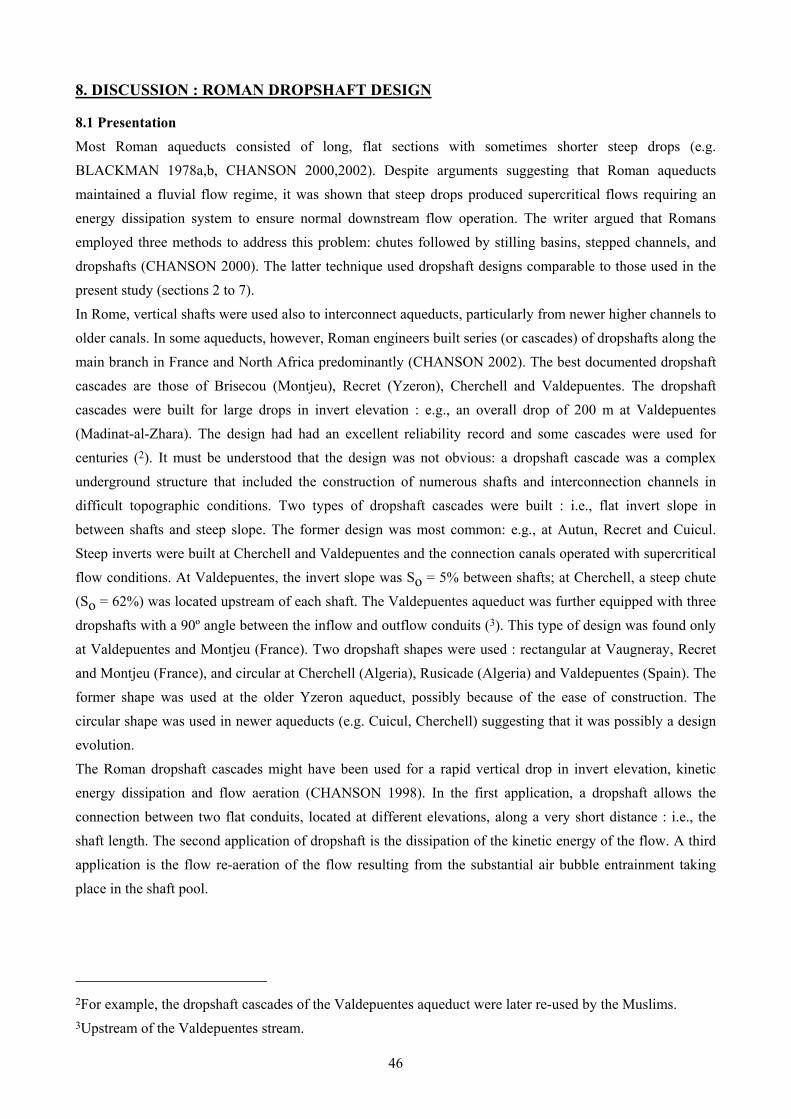
46

8. DISCUSSION : ROMAN DROPSHAFT DESIGN

8.1 Presentation Most Roman aqueducts consisted of long, flat sections with sometimes shorter steep drops (e.g. BLACKMAN 1978a,b, CHANSON 2000,2002). Despite arguments suggesting that Roman aqueducts maintained a fluvial flow regime, it was shown that steep drops produced supercritical flows requiring an energy dissipation system to ensure normal downstream flow operation. The writer argued that Romans employed three methods to address this problem: chutes followed by stilling basins, stepped channels, and dropshafts (CHANSON 2000). The latter technique used dropshaft designs comparable to those used in the present study (sections 2 to 7). In Rome, vertical shafts were used also to interconnect aqueducts, particularly from newer higher channels to older canals. In some aqueducts, however, Roman engineers built series (or cascades) of dropshafts along the main branch in France and North Africa predominantly (CHANSON 2002). The best documented dropshaft cascades are those of Brisecou (Montjeu), Recret (Yzeron), Cherchell and Valdepuentes. The dropshaft cascades were built for large drops in invert elevation : e.g., an overall drop of 200 m at Valdepuentes (Madinat-al-Zhara). The design had had an excellent reliability record and some cascades were used for centuries (2). It must be understood that the design was not obvious: a dropshaft cascade was a complex underground structure that included the construction of numerous shafts and interconnection channels in difficult topographic conditions. Two types of dropshaft cascades were built : i.e., flat invert slope in between shafts and steep slope. The former design was most common: e.g., at Autun, Recret and Cuicul. Steep inverts were built at Cherchell and Valdepuentes and the connection canals operated with supercritical flow conditions. At Valdepuentes, the invert slope was So = 5% between shafts; at Cherchell, a steep chute (So = 62%) was located upstream of each shaft. The Valdepuentes aqueduct was further equipped with three dropshafts with a 90º angle between the inflow and outflow conduits (3). This type of design was found only at Valdepuentes and Montjeu (France). Two dropshaft shapes were used : rectangular at Vaugneray, Recret and Montjeu (France), and circular at Cherchell (Algeria), Rusicade (Algeria) and Valdepuentes (Spain). The former shape was used at the older Yzeron aqueduct, possibly because of the ease of construction. The circular shape was used in newer aqueducts (e.g. Cuicul, Cherchell) suggesting that it was possibly a design evolution. The Roman dropshaft cascades might have been used for a rapid vertical drop in invert elevation, kinetic energy dissipation and flow aeration (CHANSON 1998). In the first application, a dropshaft allows the connection between two flat conduits, located at different elevations, along a very short distance : i.e., the shaft length. The second application of dropshaft is the dissipation of the kinetic energy of the flow. A third application is the flow re-aeration of the flow resulting from the substantial air bubble entrainment taking place in the shaft pool.

2For example, the dropshaft cascades of the Valdepuentes aqueduct were later re-used by the Muslims. 3Upstream of the Valdepuentes stream.

47

Despite unusual hydraulic features, Roman dropshafts were not well documented and their role was not clearly understood. CHANSON (1998,2000) presented probably the first well-documented survey of dropshafts installed along Roman aqueducts. The study is incomplete however. Fig. 8-1 - Sketch of Roman dropshaft cascades with steep conduits (e.g. Valdepuentes aqueduct, Cordoba)

8.2 Dropshafts in Roman aqueducts Although over 30 dropshaft structures were listed by CHANSON (1998,2000), some information were found subsequently to be inaccurate or misleading. Up to date, the writer has obtained detailed information and drawings of only a small number of dropshaft sites. That is, the following ten dropshafts : - Cherchell (1 dropshaft), - Valdepuentes, Cordoba, Spain (2 dropshafts) after VILLANUEVA (1993,1996), - Recret, Yzeron (2 dropshafts) (Fig. 1-3), - Vaugneray, Yzeron (1 dropshaft), - Gunudu, Tunisia (1 dropshaft), - Cologne, Germany (1 dropshaft),

48

- Montjeu, Autun (1 dropshaft) (4), - Beaulieu, Aix-en-Provence (1 dropshaft) (5). Most studies on the Montjeu aqueduct, Autun, relied on the original work of ROIDOT-DELEAGE (1879?), including PINETTE and REBOURG (1986) and CHANSON (1998,2000). Jean ROIDOT-DELEAGE (1794-1878) was an engineer at the Ponts-et-Chaussées from 1820 to 1833. He became the architect of the city of Autun in 1859, and he studied the Montdru and Montjeu aqueducts until his death. His work was published posthumously and the only remains are drawings kept at the Société Eduenne, Musée Rolin, Autun (ROIDOT-DELEAGE 1879?) (6). His drawings of the Montjeu aqueduct show 24 "puits" (or shafts), a term used for both dropshafts ("puits de rupture") and inspection shafts ("regards"). The writer inspected parts of the Montjeu aqueduct in September 2000. The path of the aqueduct is relatively flat but for two short steep sections in the Forêt de Brisecou and at Pierre de Couhard. It is the writer's opinion that the only dropshafts were the "puits" No. 18, 19, 20, 21, 22, and 24 (at Pierre de Couhard), and possibly the "puits" No. 10 and 23. The "puit" No. 10 was probably a small dropshaft. All the shafts were not identical as suggested by PINETTE and REBOURG and by CHANSON. The studies of the Valdepuentes aqueduct at Cordoba (7) showed the existence of at least three major dropshaft cascades : i.e., at Cerro de los Pinos upstream of Valdepuentes bridge, at Madinat-al-Zhara, and at Cortijo los N., downstream of junction with Veneros branch junction. The total drop in elevation at Cerro de los Pinos and Madinat-al-Zhara dropshaft cascades was respectively 120 m and 200 m. The Cerro de los Pinos dropshaft cascade was very steep (total drop of 120 m over a 400 m long distance) and an unusual spiramina design was used. It consisted of three 90-degree dropshafts. This is the only documented dropshaft design of this type. Five 90-degree shafts were possibly parts of the Montjeu aqueduct although it is uncertain whether these were dropshafts. Further observations of Roman shafts were reported, but there might be doubts whether some were wells, cisterns, inspection shafts or dropshafts (CHANSON 1998). At Cherchell, LEVEAU and PAILLET (1976) described several very-steep sections : Zabrir Clift (∆H ~ 20 m) (8), Bouchaoun gorge (∆H ~ 10 m) (9) and Oued Bellah (∆H = 37m) (10). LEVEAU and PAILLET hypothesised the existence of series of dropshafts at these three sites. As no dropshaft trace was found, it is uncertain whether the final design was dropshafts, cascades, steep chutes or a combination of different types as at Chabet Ilelouine. Near the source of the Aïn

4The original drawing by ROIDOT-DELEAGE (1879?), re-used by PINETTE and REBOURG (1986), is inaccurate. For example, the drawing of the "puit" (shaft) No. 10 is incorrect. The writer is definite after studying the original manuscript in Autun in September 2000. 5Dr P. LEVEAU questioned whether the site was a well or a dropshaft. 6No text accompanies the sketches and gravures. 7Also called Aqua Vetus. The aqueduct was used for several centuries, by the Romans and later by the Muslims. The Valdepuentes aqueduct was thoroughly studied by the engineer S. LOPEZ-CUERVO (1985) and in the Ph.D. thesis of Dr VILLANUEVA (1993,1996) who both went on site several times. 8LEVEAU and PAILLET (1976), pp. 46-47 including Fig. 24. 9LEVEAU and PAILLET (1976), pp. 56-57. 10LEVEAU and PAILLET (1976), pp. 104-107.

49

Nadour branch of the Hippo Zarite aqueduct (Tunisia), GAUCKLER (1902, pp. 126-127) observed the presence of seven circular shafts (1-m diameter, 2.5-m deep). The main channel specus was 0.2-m wide and 0.3-m high. GAUCKLER (11) described four shafts located on a steep slope (12). It is likely that these four were circular dropshafts. Six kilometres West of Zaghouan (Tunisia), GAUCKLER (1902, p. 146) described a Roman circular well (3-m diameter, over 7-m deep), feeding a 500-m long subterranean rectangular conduit. The geometry of the shaft is close to that of Chabet Ilelouine, Cherchell, suggesting possibly a dropshaft design.

8.3 Discussion The design of an aqueduct was a difficult task (GREWE 1992, HODGE 1992). In particular the hydraulic design of dropshaft was not and is still not today a simple job. It was a highly specialised task and the advice of an experienced engineer was required. GREWE (1992) and HODGE (1992) elaborated on the difficulties to design an aqueduct. The writer argued the complexity of dropshaft hydraulic calculations which today are among the most difficult. Even research on dropshaft hydraulics is limited : i.e., there are only 5 international refereed journal articles on dropshaft design listed in Science Citation Index, the Web of Science® for the period 1985-2000. The writer believes that dropshaft expertise in Roman times was restricted to a handful of engineers. Who were they ? Although there is no written proof that the engineers understood the basic concepts of continuity and energy, as used in modern hydraulics, they were contemporaries of Hero of Alexandria who understood the principle of continuity, probably those of momentum and energy (13). It is likely that he also influenced the Roman hydraulicians of the 1st, 2nd and 3rd centuries AD, and possibly, the designers of the Montjeu and Valdepuentes aqueducts. In any case, the aqueduct engineers designed reliable dropshaft structures, used for centuries (14). The sound design implied a great deal of engineering experience.

11P. GAUCKLER was the son of the famous French hydraulic engineer Philippe Gaspard GAUCKLER (1826-1905) (e.g. CHANSON 1999). 12GAUCKLER (1902), Fig. 45. 13HERO designed the first steam turbine and he impressed Italian scientists for many centuries including Galileo (LEVI 1995). 14For example, the dropshaft cascades of the Valdepuentes aqueduct were later re-used by the Muslims (VILLANUEVA 1993,1996).

50

9. CONCLUSION The hydraulics of vertical, rectangular dropshafts was systematically investigated in two prototypes and five smaller models. For two geometries, the prototype investigations were complemented by a 1:3.1 scale model study based upon an undistorted Froude similitude. Experimental observations showed three basic flow regimes for dropshaft configurations with 180º outflow direction. At low flow rates, the free jet impacted into the shaft pool (regime R1). For the largest discharges, the waters impacted onto the opposite wall (regime R3). For intermediate flow rates, the free-falling nappe entered directly into the outflow channel (regime R2). For dropshaft configurations with 90º outflow direction, the intermediate flow regime was not observed. The rate of energy dissipation was nearly 95% at low flow rates (regime R1). In models, the pool depth had little effects on the hydraulic properties of the dropshaft, but larger rate of energy dissipation was consistently observed with 90º outflow direction. Neutrally-buoyant particles were used to measure residence times in model and prototype dropshafts. In flow regime R1, and for deep shaft pools, probability distribution functions of particle residence times exhibited a bi-modal distribution in both model and prototype. Some particles plunged into the shaft pool and rapidly exited into the outflow conduit. Others remained trapped in large-scale vortical structures for up to 20 minutes. Detailed air-water flow and acoustic measurements were conducted in one prototype dropshaft under controlled flow conditions. Void fraction measurements demonstrated a strong aeration of the shaft pool for all flow regimes, but regime R2. The air-water content distributions were basically two-dimensional but next to the outer edges of the free-falling nappes. At low flow rates, void fraction distributions were successively compared with an analytical solution of the air bubble advective diffusion equation. Pseudo-bubble chord size measurements showed a broad range of entrained bubble sizes, from less than 0.5 mm to more than 25 mm, with mean pseudo-bubble chords between 10 and 20 mm. The distributions of chord sizes were skewed with a preponderance of small bubbles compared to the mean and followed a log-normal probability distribution function. Analysis of the streamwise distributions of bubbles indicated a fair proportion of bubbles associated with a cluster structure and the large majority of clusters consisted of 2 bubbles only. Acoustic signatures of the bubbly flow characterised accurately the changes in flow regimes. However the transformation from acoustic frequencies to bubble radii were inaccurate. It underestimated the entrained bubble sizes and did not predict correctly the probability distribution functions of bubble sizes. Although basic hydraulic characteristics were similar between model and prototype based upon a Froude similitude, observations of dimensionless bubble penetration depths and neutrally-buoyant particle residence times showed some discrepancies between model and prototype results. It is believed that these differences highlight the limitations of a Froude similitude for studies of air entrainment, residence times and mass transfer in dropshaft.

51

ACKNOWLEDGMENTS The writer thanks his students Joel I. WILSON and Craig RUSSELL. He thanks Dr Richard MANASSEH (CSIRO Melbourne) for his review of the report, his valuable advice on acoustic measurements, and for providing the hydrophone and the Streamtone™ software. The writer acknowledges the assistance of Graham ILLIDGE and Brendan McPHAIL.

A-1

APPENDIX A - NAPPE TRAJECTORY CALCULATIONS (AFTER CHANSON 1998)

1. Presentation For a vertical dropshaft with a horizontal upstream conduit (Fig. A-1), a simple expression for the nappe trajectory may be deduced from the motion equation assuming that the velocity of the flow at the brink of the conduit is nearly horizontal. Further developments provide information on the nappe impact conditions. Fig. A-1 - Definition sketch

Considering an aerated free-falling nappe, the flow direction at the brink of the overfall is nearly horizontal. Once the fluid leaves the canal edge, the horizontal acceleration is zero and the vertical acceleration equals minus the gravity acceleration. For a two-dimensional nappe, the jet velocity components in the x- and y-directions are : Vx = Vb (A-1a)

Vy = - g * t (A-1b)

A-2

where Vb is the flow velocity at the brink of the step and t is the time. The trajectory equation of the nappe centreline is : x = Vb * t (A-2a)

y = h + db2 -

12 * g * t2 (A-2b)

where h is the drop height and db is the flow depth at the brink. Once the fluid leaves the step, the time t', taken to hit the opposite wall (x = L - l), is given by :

t' = L - lVb

(A-3)

The vertical location of the nappe impact on the opposite wall (x = L - l) equals :

y = h + db2 -

12 * g *

L - l

Vb

2 (A-4)

2. Applications to Roman dropshaft When the nappe impacts into the shaft pool (i.e. regime R1), the flow conditions at impact may be derived from the trajectory equation. Once the fluid leaves the step, the time t" taken to reach the pool free-surface is given by :

yp =

h + db2 -

12 * g * t"2 (A-5)

where yp is the water elevation in the pool behind the overfalling jet. The nappe thickness di and the flow velocity Vi at the intersection of the falling nappe with the receiving pool are then :

didc

=

dc

db

2 + 2 *

h + db2 - ypdc

-1/2

(A-6)

ViVc

=

dc

db

2 + 2 *

h + db2 - ypdc

(A-7)

The angle of the falling nappe with the horizontal is given by :

tanθ = 2 * dbdc

* h +

db2 - ypdc

(A-8)

Nappe impact on the downstream channel invert (Case 1) Nappe impact into the downstream conduit occurs when x = (L - l) and 0 ≤ y ≤ D simultaneously (Eq. (A-2)). The flow conditions for the limiting conditions {x = L - l, y = 0} are deduced from the solution of a polynomial equation of degree two. The solution is :

A-3

Vb

g * (L - l) =

12 *

hL - l *

8 *

L - lh +

Q2

g*b2*h2*(L - l) -

Q

g*b2*h2*(L - l) = X1

{x = L - l, y = 0} (A-9a)

assuming that h > 0, where Q is the total flow rate and b is the brink channel width. For Vb < g*(L - l)*X1

, the nappe impacts in the pool, short of the inlet invert (i.e. regime R1). Note that Equation (A-9) may be rewritten as :

Vb

g * (L - l) =

12 *

hL - l *

8 * L - l

h + dc

3

h2*(L - l) -

dc3/2

h2*(L - l) = X1

{x = L - l, y = 0} (A-9b)

where dc is the critical depth at the step brink : dc = 3

Q2/(g*b2). In terms of the brink flow depth, it yields:

dbdc

= 12 *

dc

L - l

2 *

1 + 8 * hdc

*

L - l

dc

2 {x = L - l, y = 0} (A-10)

Nappe impact on the downstream channel obvert (Case 2) Nappe impact on the inlet obvert occurs for x = (L - l) and y = D simultaneously (Eq. (A-2)), provided that (h - D) is positive. The flow conditions for such a situation are deduced from the solution of a polynomial equation of degree two. The solution is :

Vbg * (L - l)

= 12 *

h - DL - l *

8 *

L - lh - D +

Q2

g*b2*(h-D)2*(L - l) -

Q

g*b2*(h- D)2*(L - l) = X2

{x = L - l, y = D} (A-11)

assuming that h > D. For Vb > g*(L - l)*X2, the nappe impacts the opposite wall above the inlet obvert.

In terms of the brink flow depth, it yields :

dbdc

= 12 *

dc

L - l

2 *

1 + 8 * h - D

dc *

L - l

dc

2 {x = L, y = D} (A-12)

Particular case : subcritical aqueduct flows The above development (Eq. (A-9) to (A-12)) is general to any two-dimensional inflow. In the particular case of a subcritical inflow, critical flow conditions occur at the brink of the overfall (e.g. HENDERSON 1966, pp. 28 &192; COMOLET 1976, p. 357). With subcritical upstream flow, the flow depth db at the brink of the overfall (x = 0, y = h) is directly related to the critical flow depth and hence the flow rate. Table A-2 reviews experimental and analytical estimates. For engineering applications, ROUSE's (1936) result is commonly accepted :

db = 0.715 * dc = 0.715 * 3 Q2

g*b2 (A-13)

where b is the inflow chanel width at the brink.

A-4

Combining Equation (A-13) with Equations (A-10) and (A-12) yields two dimensionless relationships between h, L, D and dc :

h

L - l = 12 *

L - ldc

*

db

dc

2 -

12 *

dbdc

* dc

L - l {x = L - l, y = 0} {Case 1} (A-14)

h - DL - l =

12 *

L - ldc

*

db

dc

2 -

12 *

dbdc

* dc

L - l {x = L - l, y = D} {Case 2} (A-15)

where db/dc is a constant smaller than unity (i.e. db/dc = 0.7). Note a simpler approximate expression obtained for the lower nappe :

h

L - l = 12 *

L - ldc

*

db

dc

2 {x = L - l, y = 0} {Case 1} (A-14b)

h - DL - l =

12 *

L - ldc

*

db

dc

2 {x = L - l, y = D} {Case 2} (A-15b)

Analytical model validation Calculations were compared with CHANSON's (2002) data (Models 1, 2, and 3, Table 2-1). The results were satisfactory and validated the analytical model for both subcritical and supercritical inflow conditions.

A-5

APPENDIX B - EXPERIMENTAL RESULTS (1) HYDRAULIC PERFORMANCES Hydraulic tests were conducted for 5 model configurations and 2 prototype configurations (Table B-1). Table B-1 - Experimental investigations of rectangular dropshafts

Ref. h P L B l b1 D1 (1) b2 D2 Outflow direction

Remark

m m m m m m m m m deg. (1) (2) (3) (4) (5) (6) (7) (8) (9) (10) (11) (12)

Present 2.70 0 0.755 0.763 0.12 0.50 0.30 0.65 0.20 90 Prototype P1. study 1.70 1.00 0.755 0.763 0.12 0.50 0.30 0.50 0.30 180 Prototype P2. 0.87 0 0.243 0.246 0.039 0.161 0.25 0.209 0.064 90 Model 4. 0.548 0.322 0.243 0.246 0.039 0.161 0.25 0.209 0.097 180 Model 5. 0.548 0.322 0.243 0.246 0.039 0.161 0.25 0.209 0.097 90 Model 6. 0.548 0 0.243 0.246 0.039 0.161 0.25 0.209 0.097 180 Model 7. 0.548 0 0.243 0.246 0.039 0.161 0.25 0.209 0.097 90 Model 8. CHANSON 0.505 0.365 0.30 0.30 0 0.144 0.25 0.15 0.25 180 Recret model. (2002) 0.668 0.201 0.20 0.30 0 0.110 0.25 0.11 0.21 90 Valdepuentes

model 1. 0.668 0.201 0.20 0.30 0 0.110 0.25 0.11 0.21 180 Valdepuentes

model 2. APELT (1984)

0.325 0 0.152 0.152 0 Pipe : Ø = 0.152 m

Pipe : Ø = 0.152 m

180

Notes : (1) : sidewall height; Notation : see Figure 2-1. Notation b1 inflow channel brink width (m); Dab bubble penetration depth (m), measured vertically from the pool free-surface; D2 downstream conduit height (m); dc critical depth at the inflow flume brink (m); dp pool depth (m); H1 upstream total head (m) measured above the downstream conduit invert; H2 downstream specific energy (m), or residual head; h drop in invert elevation (m); Q water discharge (m3/s); Q' dimensionless flow rate : Q' = Q/ g*b12*D23;

P shaft pool height (m); yp pool depth (m) measured above the downstream channel invert (m) : yp = dp - P;

A-6

B.1 Model data (University of Queensland)

Location : University of Queensland (Australia) Date : Mar-June 2002 Experiments by : C. RUSSELL and J. WILSON Data processing by : C. RUSSELL, J. WILSON and H. CHANSON Experiment characteristics :

Inflow flume : length: 3.2 m, width: 0.25 m, slope: 0 degrees (horizontal), brink width: 0.161 m. Open channel with glass sidewalls. Shaft : rectangular shaft (plywood and perspex). Outflow channel : rectangular conduit (plywood and perspex).

Instrumentation : Pointer gauges, rulers, total head tube (Ø = 1 mm). Comments : Broad-crested weir located upstream of sidewall contraction. Sub-critical

shaft inflow conditions (i.e. subcritical flow upstream of sidewall contraction).

Model 4

Q' dch

ypD

H2H1

(1) (2) (3) (4) 0.011 0.005 0.091 0.004 0.017 0.007 0.136 0.006 0.026 0.009 0.273 0.018 0.030 0.010 0.258 0.016 0.038 0.011 0.273 0.017 0.046 0.013 0.333 0.019 0.054 0.015 0.303 0.022 0.073 0.018 0.455 0.028 0.082 0.019 0.455 0.035 0.088 0.020 0.348 0.034 0.109 0.023 0.485 0.040 0.126 0.025 0.545 0.038 0.131 0.026 0.561 0.044 0.155 0.029 0.712 0.047 0.187 0.033 0.909 0.047 0.227 0.038 0.894 0.053 0.255 0.041 0.909 0.058 0.284 0.044 0.970 0.061 0.330 0.049 1.000 0.068 0.402 0.055 1.136 0.071 0.427 0.058 1.136 0.073 0.496 0.064 1.242 0.089 0.532 0.067 1.379 0.087 0.569 0.070 1.439 0.088 0.606 0.073 1.576 0.100 0.644 0.076 1.697 0.098 0.683 0.079 1.788 0.107 0.722 0.082 1.788 0.114 0.742 0.083 1.773 0.109 0.783 0.086 1.909 0.124 0.824 0.089 2.045 0.117 0.866 0.092 2.167 0.133 0.908 0.095 2.273 0.140 0.951 0.098 2.333 0.167 1.017 0.103 2.470 0.199 1.062 0.106 2.652 0.206

Model 5

Q' dch

Dabdp

ypD

H2H1

(1) (2) (3) (4) (5) 0.008 0.009 0.161 0.041 0.007 0.009 0.010 0.378 0.052 0.011 0.013 0.013 0.639 0.062 0.013 0.019 0.017 0.646 0.072 0.016 0.028 0.022 0.827 0.093 0.025 0.035 0.025 0.872 0.103 0.030 0.046 0.030 0.941 0.144 0.033 0.052 0.033 0.928 0.196 0.033 0.058 0.035 1.000 0.247 0.042 0.064 0.037 0.957 0.247 0.064 0.067 0.039 1.000 0.268 0.057 0.070 0.040 0.637 0.278 0.199 0.070 0.040 0.986 0.247 0.136 0.080 0.044 0.275 0.278 0.248 0.084 0.045 0.381 0.268 0.217 0.087 0.046 0.257 0.330 0.262 0.091 0.047 0.298 0.371 0.211 0.091 0.047 0.307 0.371 0.143 0.101 0.051 0.458 0.443 0.159 0.101 0.051 0.488 0.443 0.220 0.112 0.054 0.583 0.474 0.238 0.124 0.058 0.650 0.495 0.243 0.131 0.060 0.710 0.515 0.247 0.143 0.064 0.763 0.557 0.244 0.160 0.069 0.796 0.588 0.238 0.181 0.075 0.790 0.619 0.218 0.198 0.080 0.806 0.670 0.207 0.216 0.084 0.794 0.753 0.210 0.230 0.088 0.791 0.835 0.208 0.230 0.088 0.780 0.856 0.214 0.254 0.094 0.779 0.928 0.219 0.259 0.095 0.784 0.928 0.231 0.274 0.099 0.788 0.959 0.236 0.294 0.103 0.778 1.041 0.251 0.309 0.107 0.777 1.082 0.262 0.330 0.112 0.745 1.134 0.268 0.345 0.115 0.799 1.155 0.278

0.361 0.119 0.867 1.216 0.288 0.383 0.123 0.898 1.289 0.297 0.400 0.127 0.907 1.381 0.306 0.422 0.132 0.957 1.433 0.313 0.451 0.138 0.985 1.454 0.322 0.474 0.142 1.000 1.505 0.332 0.492 0.146 1.000 1.588 0.341 0.516 0.151 1.000 1.722 0.354 0.534 0.154 1.000 1.784 0.360 0.558 0.159 1.000 1.866 0.365

Model 6

Q' dch

Dabdp

ypD

H2H1

(1) (2) (3) (4) (6) 0.006 0.008 0.135 0.072 0.011 0.009 0.010 0.375 0.072 0.018 0.017 0.015 0.687 0.093 0.021 0.026 0.020 0.801 0.113 0.027 0.033 0.024 0.851 0.175 0.032 0.038 0.026 0.879 0.206 0.035 0.046 0.030 1.000 0.268 0.039 0.058 0.035 1.000 0.289 0.043 0.070 0.040 1.000 0.320 0.048 0.084 0.045 1.000 0.392 0.054 0.098 0.050 1.000 0.402 0.059 0.112 0.054 1.000 0.464 0.065 0.127 0.059 1.000 0.505 0.068 0.143 0.064 1.000 0.515 0.071 0.160 0.069 1.000 0.546 0.077 0.176 0.074 1.000 0.588 0.084 0.194 0.078 1.000 0.619 0.088 0.212 0.083 1.000 0.639 0.092 0.230 0.088 1.000 0.691 0.097 0.249 0.093 1.000 0.753 0.101 0.269 0.097 1.000 0.804 0.103 0.294 0.103 1.000 0.835 0.107 0.319 0.109 1.000 0.907 0.111 0.340 0.114 1.000 0.959 0.115 0.367 0.120 1.000 0.990 0.119 0.394 0.126 1.000 1.041 0.129

A-7

0.428 0.133 1.000 1.113 0.140 0.462 0.140 1.000 1.165 0.152 0.498 0.147 1.000 1.268 0.166 0.534 0.154 1.000 1.371 0.175 0.571 0.161 1.000 1.536 0.183

Model 7

Q' dch

ypD

H2H1

(1) (2) (3) (4) 0.009 0.010 0.052 0.016 0.019 0.017 0.196 0.030 0.030 0.023 0.186 0.042 0.055 0.034 0.237 0.068 0.074 0.041 0.289 0.213 0.105 0.052 0.598 0.176

0.127 0.059 0.619 0.182 0.176 0.074 0.763 0.207 0.221 0.086 0.876 0.224 0.274 0.099 1.093 0.232 0.319 0.109 1.247 0.269 0.372 0.121 1.392 0.291 0.428 0.133 1.588 0.310 0.474 0.142 1.784 0.329 0.609 0.168 2.309 0.391

Model 8

Q' dch

ypD

H2H1

(1) (2) (3) (4) 0.006 0.008 0.134 0.016 0.011 0.012 0.144 0.021

0.017 0.015 0.175 0.025 0.026 0.020 0.216 0.039 0.041 0.028 0.289 0.045 0.058 0.035 0.320 0.066 0.074 0.041 0.351 0.081 0.105 0.052 0.567 0.091 0.151 0.066 0.639 0.103 0.203 0.081 0.732 0.107 0.259 0.095 0.814 0.118 0.309 0.107 0.918 0.126 0.351 0.116 1.010 0.135 0.405 0.128 1.165 0.148 0.451 0.138 1.289 0.169 0.498 0.147 1.371 0.188 0.546 0.156 1.515 0.254

B.2 Prototype data (University of Queensland)

Location : University of Queensland (Australia) Date : June-Aug. 2002 Experiments by : C. RUSSELL and J. WILSON Data processing by : C. RUSSELL, J. WILSON and H. CHANSON Experiment characteristics :

Inflow flume : length: 12 m, width: 0.5 m, slope: 0 degrees (horizontal), brink width: 0.5 m. Open channel with glass sidewalls. Shaft : rectangular shaft (plywood and perspex). Outflow channel : rectangular conduit (plywood and perspex).

Instrumentation : Pointer gauges, rulers, total head tube (Ø = 1 mm). Comments : Sub-critical inflow conditions.

Prototype P1

Q' dch

ypD

H2H1

(1) (2) (3) (4) 0.013 0.006 0.017 0.012 0.015 0.006 0.030 0.017 0.020 0.007 0.057 0.023 0.024 0.008 0.061 0.022 0.030 0.010 0.078 0.022 0.033 0.010 0.091 0.030 0.037 0.011 0.100 0.026 0.045 0.013 0.104 0.040 0.052 0.014 0.113 0.045 0.065 0.016 0.139 0.045 0.084 0.019 0.183 0.060 0.097 0.021 0.217 0.057 0.102 0.022 0.235 0.052 0.108 0.023 0.257 0.056 0.125 0.025 0.391 0.059 0.134 0.026 0.513 0.059 0.152 0.029 0.565 0.064 0.204 0.035 0.696 0.078 0.238 0.039 0.770 0.085

0.279 0.043 0.822 0.080 0.313 0.046 0.861 0.082

Prototype P2

Q' dch

Dabdp

ypD

H2H1

(1) (2) (3) (4) (5) 0.004 0.002 0.1317 0.000 0.007 0.005 0.004 0.1618 0.000 0.0084 0.007 0.004 0.2119 0.003 0.0103 0.010 0.007 0.282 0.010 0.0144 0.013 0.009 0.3514 0.020 0.0174 0.015 0.011 0.3704 0.030 0.0193 0.019 0.012 0.3896 0.037 0.0208 0.026 0.017 0.4291 0.040 0.0248 0.038 0.020 0.4658 0.063 0.0312 0.048 0.023 0.4907 0.097 0.0397 0.058 0.027 0.3791 0.217 0.0426 0.076 0.031 0.4587 0.333 0.0782 0.086 0.035 0.471 0.380 0.1096 0.093 0.036 0.4991 0.373 0.1389 0.101 0.038 0.45 0.403 0.1775

0.113 0.042 0.2667 0.450 0.2178 0.123 0.044 0.2193 0.500 0.2228 0.132 0.046 0.35 0.510 0.183 0.147 0.050 0.4255 0.617 0.1879 0.165 0.054 0.4878 0.663 0.1999 0.178 0.057 0.5338 0.697 0.2182 0.200 0.061 0.5738 0.767 0.2321 0.212 0.064 0.5714 0.783 0.2356 0.225 0.067 0.5654 0.827 0.2441 0.245 0.070 0.5835 0.870 0.2478 0.264 0.074 0.6181 0.907 0.2593 0.270 0.075 0.6403 0.917 0.2615

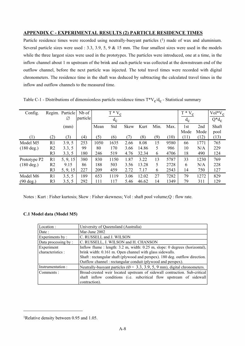
A-8

APPENDIX C - EXPERIMENTAL RESULTS (2) PARTICLE RESIDENCE TIMES Particle residence times were recorded using neutrally-buoyant particles (1) made of wax and aluminium. Several particle sizes were used : 3.3, 3.9, 5, 9 & 15 mm. The four smallest sizes were used in the models while the three largest sizes were used in the prototypes. The particles were introduced, one at a time, in the inflow channel about 1 m upstream of the brink and each particle was collected at the downstream end of the outflow channel, before the next particle was injected. The total travel times were recorded with digital chronometers. The residence time in the shaft was deduced by subtracting the calculated travel times in the inflow and outflow channels to the measured time. Table C-1 - Distributions of dimensionless particle residence times T*Vc/dc - Statistical summary Config. Regim. Particle

∅ Nb of

particle T * Vc

dc

T * Vcdc

Vol*Vc

Q*dc

(mm) Mean Std Skew Kurt Min. Max. 1st Mode

2nd Mode

Shaft pool

(1) (2) (3) (4) (5) (6) (7) (8) (9) (10) (11) (12) (13) Model M5 R1 3.9, 5 253 1050 1635 2.66 8.08 15 9580 66 1771 765 (180 deg.) R2 3.3, 5 99 80 170 3.66 14.86 5 986 10 N/A 229 R3 3.3, 5 180 246 519 4.76 32.34 6 4706 18 490 124 Prototype P2 R1 5, 9, 15 380 830 1150 1.87 3.22 13 5787 33 1230 769 (180 deg.) R2 9.15 86 188 503 3.56 13.28 5 2728 6 N/A 228 R3 5, 9, 15 227 209 459 2.72 7.17 6 2543 14 750 127 Model M6 R1 3.5, 5 189 653 1119 3.06 12.02 27 7282 79 1272 829 (90 deg.) R3 3.5, 5 292 111 117 5.46 46.62 14 1349 79 311 129

Notes : Kurt : Fisher kurtosis; Skew : Fisher skewness; Vol : shaft pool volume;Q : flow rate.

C.1 Model data (Model M5)


Inflow flume : length: 3.2 m, width: 0.25 m, slope: 0 degrees (horizontal), brink width: 0.161 m. Open channel with glass sidewalls. Shaft : rectangular shaft (plywood and perspex). 180 deg. outflow direction. Outflow channel : rectangular conduit (plywood and perspex).

Instrumentation : Neutrally-buoyant particles (Ø = 3.3, 3.9, 5, 9 mm), digital chronometers. Comments : Broad-crested weir located upstream of sidewall contraction. Sub-critical


1Relative density between 0.95 and 1.05.

A-9

Model M5, Regime R1

Run T*Vcdc

(1) (2) Ball1 92.9 (=5mm) 439.7 Regime 152.1 R1b 16.8

(just R1b)

925.9

Q = 1.626

334.0

L/s 105.6 1031.6 25.3 97.2 35.8 245.2 270.5 21.0 38.0 31.6 50.6 397.4 18.9 1052.8 95.0 65.4 545.4 171.2 27.4 84.5 46.4 862.5 1856.2 460.8 883.6 312.8 76.0 33.7 1306.5 18.9 16.8 40.1 97.2 334.0 672.2

Ball2 33.7 (3.9mm) 270.5 Regime 33.7 R1b 42.2

(just R1b)

186.0

Q = 1.626

23.2

L/s 33.7 14.7 27.4 1095.1 42.2 566.5 27.4

31.6 54.9 23.2 27.4 207.1 50.6 76.0 116.2 71.8 947.1 122.5 23.2 1877.3 35.8 31.6 1137.4 29.5 841.4 545.4 42.2 107.7 1919.6 38.0 756.8 46.4 82.4 1221.9 76.0 71.8

Ball1 538.5 (5mm) 1122.1 Regime R1a

1020.6

Q = 0.941 L/s

81.8

4547.7 487.8 1680.4 538.5 1553.5 58.9 76.7 91.9 690.8 1629.6 53.9 1502.8 1553.5 1147.5 41.2 1452.0 1020.6 58.9 5537.4 589.3 310.2 114.8 3761.1 1426.6 1020.6 1858.0 1096.8 766.9 234.0 5182.1 1274.4 1781.9 61.5

74.2 1528.1 58.9 1832.6 183.3 487.8 1756.5 1020.6

Ball2 437.0 (3.9mm) 69.1 Regime R1a

3253.6

Q = 0.941 L/s

5740.4

259.4 119.8 5867.2 3228.3 1020.6 84.3 3456.6 2619.3 53.9 124.9 1375.9 614.7 58.9 716.2 1299.8 61.5 360.9 81.8 817.7 94.5 716.2 284.8 563.9 66.6 6552.4 640.0

Ball1 72.3 (5mm) 128.0 Regime R1b ??

1121.4

Q=0.436 L/s

72.3

8957.1 1613.2 1383.7 1187.0 760.8 98.5 82.1 3154.1 891.9 924.7 105.1 2924.6 3678.7 4104.9 3350.8 2236.1 69.0 3285.2 1875.5 1416.5 55.9 1547.6

1383.7 82.1 95.2 85.4 95.2 482.1 59.2 82.1 8399.7 2367.2 891.9 55.9 75.5 91.9 465.7 301.8 75.5 301.8 1842.7 105.1 269.0 4793.4 2006.6 72.3 65.7

Ball2 1711.5 (3.9mm) 4662.2 Regime R1b ??

2531.2

Q=0.436 L/s

1580.4

1055.8 72.3 72.3 1252.5 1088.6 105.1 3875.4 39.5 72.3 105.1 3350.8 695.2 39.5 2105.0 111.6 2727.9 760.8 4727.8 9580.0 957.5 144.4 88.7 629.6 6990.0 564.1 105.1 1482.0 105.1 72.3 2465.6 367.3 301.8 4662.2 105.1 1350.9 1777.1 72.3

3285.2 334.6 7776.8

Model M5, Regime R2 Q = 1.853 L/s

Run T*Vcdc

(1) (2) Ball1 8.74 (5mm) 16.83

6.71 217.20 142.32 10.76 6.71 12.79 18.86 8.74 14.81 12.79 10.76 4.69 14.81 14.81 8.74 10.76 12.79 4.69 26.95 22.91 945.81 33.03 14.81 20.88 10.76 12.79 18.86 136.25 12.79 4.69

Ball2 51.24 3.9mm 16.83

192.92 20.88 12.79 26.95 24.93 22.91 10.76 460.07 33.03 8.74 28.98 6.71 10.76 37.07 419.59 20.88

A-10

16.83 298.16 10.76 20.88 26.95

Ball3 51.24 3.3mm 14.81

581.51 59.34 35.05 217.20 75.53 16.83 8.74 12.79 138.27 10.76 37.07 20.88 24.93 196.96 16.83 14.81 10.76 18.86 33.03 24.93 986.29 142.32 16.83 24.93 10.76 14.81 10.76 28.98 358.88 20.88 12.79 8.74 6.71 16.83 277.92 22.91 4.69 122.08 18.86 520.79 16.83 8.74

Model M5, Regime R3

Run T*Vcdc

(1) (2) Ball1 40.46 (3.3mm) 4706.03 Q=2.589 L/s

1374.77

Regime R3a (just R3a from R2)

20.54

36.83 415.22 360.91 13.30 15.11 686.79 614.37 24.16 16.92 13.30 904.05 541.96 16.92 11.49 9.68 20.54 2171.38 18.73 27.78 20.54 614.37 11.49 69.42 2388.63 49.51 20.54 47.70 13.30 487.64 15.11 54.94 1374.77 234.18 578.16

7.87 38.65 45.89 18.73 487.64 20.54

Ball2 360.91 (=5mm) 27.78 Q=2.589 L/s

15.11

Regime R3a (just R3a from R2)

18.73

469.54 1465.29 24.16 13.30 9.68 560.06 723.00 20.54 13.30 1447.19 614.37 24.16 451.43 9.68 6.06 16.92 13.30 15.11 18.73 11.49 27.78 74.85 13.30 13.30 15.11 451.43 15.11 234.18 560.06 11.49 47.70 13.30 1465.29 11.49 9.68 18.73 15.11 152.70

415.22 16.92 1266.14

Ball1 46.08 (3.3mm) 28.68 Regime R3a

1060.50

Q=3.877 L/s

35.01

380.00 1487.79 66.66 46.08 19.18 12.85 69.82 22.35 316.70 6.52 50.83 12.85 17.60 19.18 128.38 601.56 1076.33 50.83 72.99 664.86 44.50 42.92 522.43 205.92 28.68 76.15 30.26 54.00 395.83 85.65 174.27 35.01 20.76 11.27 11.27 28.68 33.42 538.26 348.35 57.16 17.60

Ball2 22.35

(5mm) 22.35 Regime R3a

28.68

Q=3.877 L/s

23.93

28.68 12.85 20.76 41.34 39.75 22.35 17.60 441.72 17.60 17.60 20.76 23.93 506.61 316.70 27.09 16.02 14.43 443.31 28.68 155.28 190.10 14.43 601.56 474.96 16.02 9.69 20.76 17.60 12.85 9.69 411.65 14.43 14.43 14.43 35.01 27.09 14.43 31.84 316.70 19.18 712.34 36.59

C.2 Prototype data (Prototype P2)

Location : University of Queensland (Australia) Date : June-Aug. 2002 Experiments by : C. RUSSELL and J. WILSON Data processing by : C. RUSSELL, J. WILSON and H. CHANSON Experiment characteristics :

Inflow flume : length: 12 m, width: 0.5 m, slope: 0 degrees (horizontal), brink width: 0.5 m. Open channel with glass sidewalls. Shaft : rectangular shaft (plywood and perspex). 180 deg. outflow direction. Outflow channel : rectangular conduit (plywood and perspex).

Instrumentation : Neutrally-buoyant particles (Ø = 5, 9 & 15 mm), digital chronometers. Comments : Sub-critical inflow conditions.

A-11

Prototype P2, Regime R1

Run T*Vcdc

(1) (2) Ball1 3716.40 (9mm) 41.16 Regime R1b

3272.71

Q=7.6 L/s

48.55

48.55 50.40 869.38 1479.46 2588.68 518.13 536.61 59.65 111.41 1183.66 1294.59 776.95 1146.69 5195.37 92.92 869.38 4215.55 388.72 943.33 3642.45 869.38 4215.55 388.72 943.33 3642.45 26.37 1886.17 3402.12 61.49 629.05 2163.48 24.52 22.67 721.48 703.00 1109.71 5694.52 30.07 573.59 24.52 3328.17 296.28 592.07 26.37 72.59 1257.61 44.86 277.79 3790.35 37.46 92.92 3050.86

Ball2 5361.75 (15mm) 1054.25 Regime R1b

59.65

Q=7.6 L/s

481.15

33.76 37.46 111.41 59.65 333.25 41.16 41.16 2052.56 3291.20 222.33 3457.58 59.65 610.56 3272.71 1701.30 1978.61 3660.94 70.74 2348.35 2644.15 65.19 1719.79 5786.96 28.22 41.16 3087.84 28.22 96.62

5mm 12.62 Regime R1b

2034.94

Q=16 L/s 116.48 87.63 2986.95 32.82 22.72 1544.50 2857.13 534.79 18.39 765.58 563.64 32.82 1299.29 1284.86 45.80 1732.02 37.14 3304.29 38.59 32.82 44.36 505.94 606.91 2698.46 38.59 50.13 18.39 41.47 27.05 37.14 246.30

44.36 1631.05 41.47 909.83 1169.47 260.72 50.13 433.82 1717.60 102.05 289.57 48.68 1746.45


25.60

Q=16 L/s 981.95 116.48 32.82 1775.30 751.16 390.54 174.18 549.21 2236.88 275.15 635.76 332.85 47.24 246.30 1183.89 87.63 1111.77 520.36 35.70 174.18 1140.62 289.57 679.03 1746.45 67.43 203.02 679.03 32.82 28.49 54.45 38.59 2785.01 2352.28 50.13 3751.45 73.20 390.54 25.60 332.85 246.30 477.09 1804.14 664.61 1631.05 549.21 2063.79 29.93 549.21


880.98

Q=16 L/s 462.67

260.72 664.61 390.54 21.28 2770.59 41.47 42.91 520.36 1256.01 116.48 895.40 967.52 246.30 159.75 1183.89 1905.12 2323.43 679.03 45.80 188.60 51.57 1371.41 1948.39 534.79 3419.69 145.33 1256.01 1111.77 246.30 84.74 217.45 217.45 1198.32 332.85 981.95 563.64 1501.23 73.20 404.97 217.45 361.69 563.64 1919.54 765.58 1342.56 419.39 116.48

5mm 32.72 Regime R1b (almost R2)

32.72

Q=24 L/s 1286.52 21.38 1009.30 21.38 4247.75 23.90 26.42 25.16 84.39 18.86 1084.90 51.63 669.07 23.90 1210.91 127.23

1210.91 757.28 27.68 845.49 32.72 543.06 316.25 429.65 26.42 480.06 2244.19 2735.63 26.42 1248.72 228.04 2798.63 20.12 152.43 18.86 2181.19 23.90 23.90 21.38 2924.64 20.12 22.64 94.47 618.67 22.64 3227.07


55.41

Q=24 L/s 1677.15 56.67 127.23 64.23 3605.10 454.86 3390.88 25.16 27.68 28.94 33.98 32.72 4701.38 152.43 1488.13 68.01 618.67 20.12 20.12 215.44 1009.30 33.98 2584.42 55.41 681.67 22.64 64.23 25.16 2622.22 21.38 2622.22 21.38 1097.51

A-12

15.08 61.71 1223.51 1803.16 21.38 3907.52 42.80 42.80 278.44 4449.36 18.86 94.47 18.86 33.98


66.75

Q=24 L/s 568.26 45.33 45.33 18.86 404.45 46.59 202.84 78.09 1236.12 44.06 1399.93 13.82 40.28 42.80 32.72 21.38 656.47 631.27 883.29 694.27 1425.13 18.86 656.47 21.38 20.12 55.41 1034.50 580.87 3012.85 28.94 845.49 1588.94 20.12 55.41 25.16 1110.11 517.86 732.08 480.06 984.10 18.86 20.12 21.38 21.38 18.86 94.47 114.63

Prototype P2, Regime R2 Q = 33 L/s

Run T*Vcdc

(1) (2) Ball1 14 (=9mm)

13

326 14 1289 824 8 10 11 15 11 2467 1006 1312 11 1980 33 13 15 11 12 6 10 269 13 14 13 12 22 12 12 10 11 14 39 10 348 14 5 7 12 17

Ball2 10 (=15mm)

6

586 11 11 12 12 16 6 12 19

7 8 10 25 12 7 609 371 10 8 14 8 779 11 6 8 2728 13 11 473 11 7 10 8 7 13 6 6 16 8 6 6 6

Prototype P2, Regime R3

Run T*Vcdc

(1) (2) 5mm 6.76 Regime R3a

9.83

Q=45 L/s 26.18 29.24 15.96 18.00 21.07 45.59 24.14 13.92 15.96 16.98 1429.23 2052.58 12.89 601.50 1327.04 14.94 18.00 11.87 20.05 8.81 18.00

21.07 315.37 10.85 18.00 28.22 652.60 8.81 9.83 14.94 14.94 10.85 2001.49 10.85 13.92 19.03 19.03

9mm 9.83 Regime R3a

9.83

Q=45 L/s 1214.63 2124.11 18.00 1562.08 16.98 1030.69 11.87 15.96 9.83 1153.32 18.00 1255.51 12.89 1122.66 18.00 264.28 10.85 10.85 1940.17 10.85 13.92 10.85 10.85 12.89 325.59 16.98 16.98 14.94 14.94 12.89 1490.54 8.81 8.81 16.98 826.32 10.85 41.51 10.85

15mm 6.76 Regime R3a

60.92

Q=45 L/s 12.89 243.84 10.85 10.85 11.87 11.87 14.94

14.94 10.85 14.94 9.83 9.83 11.87 182.53 5.74 397.12 1255.51 2543.09 529.97 1214.63 15.96 1194.20 16.98 21.07 13.92 16.98 11.87 13.92 18.00 356.25 19.03 417.56 10.85 13.92 31.29 1112.45 14.94 785.44


14.58

Q=67L/s 10.10 18.16 19.05 19.05 15.47 19.05 448.61 20.84 28.00 19.05 20.84 18.16 14.58 19.05


12.79

Q=67L/s 8.31 12.79 10.10 11.89 14.58 19.95 9.21 788.68 11.00 90.64 11.89 1191.39 10.10 582.85 14.58 887.12 16.37

A-13

1424.07 9.21 11.00 13.68 28.00 11.00 171.19 23.53 332.27 12.79 251.73 11.00 12.79 11.00 242.78 11.89

16.37 14.58 14.58 11.89 14.58 9.21 9.21 9.21 10.10 9.21 11.89


29.79

Q=67L/s 9.21 26.21

11.00 99.59 13.68 1397.22 9.21 162.24 19.05 9.21 9.21 12.79 12.79 10.10 11.00 13.68 41.42 7.42

251.73 10.10 10.10 15.47 457.56 11.89 15.47 11.00 12.79 11.89 260.68 10.10 162.24 11.00 538.10 10.10

36.95 1245.09 11.00 189.08 13.68 466.51 10.10 11.00 46.79 135.39

C.3 Model data (Model M6)


Inflow flume : length: 3.2 m, width: 0.25 m, slope: 0 degrees (horizontal), brink width: 0.161 m. Open channel with glass sidewalls. Shaft : rectangular shaft (plywood and perspex). 90-deg. outflow direction. Outflow channel : rectangular conduit (plywood and perspex).

Instrumentation : Neutrally-buoyant particles (Ø = 3.5, 5 mm), digital chronometers. Comments : Broad-crested weir located upstream of sidewall contraction. Sub-critical


Model M6, Regime R1

Run T*Vcdc

(1) (2) Regime

R1b 2204.1

Q = 0.44 L/s

3449.0

Particle Ø

3907.7

3.7 & 5 mm

1188.4

1810.9 58.1 113.8 54.8 598.7 467.7 2433.4 2597.2 1843.7 94.2 58.1 434.9 68.0 3186.9 77.8

3776.6 697.0 2728.3 1450.5 41.7 1974.7 434.9 87.6 107.3 2007.5 130.2 1876.4 71.2 2269.6 2892.1 2924.8 795.3 271.1 231.8 762.5 238.3 402.1 1942.0 860.8 926.3 51.6 991.8 434.9 48.3 565.9 84.3 926.3

795.3 729.8 71.2 153.1 467.7 1286.7 2695.5 45.0 7282.2 120.4 893.6 1712.6 205.6 271.1 107.3 7020.1 4104.3 94.2 74.5 893.6 303.8 369.4 1024.6 271.1 271.1 117.1 48.3 2073.0 1385.0 3219.7 2335.1 828.0

3416.3 238.3 1942.0 1090.1 208.8 74.5 336.6 369.4 1090.1 1221.2 1516.0 1450.5 369.4 77.8 113.8 84.3 48.3

Regime R1b

95.2

Q = 0.94 L/s

357.2

Particle size

107.9

3.5 & 5 mm

118.1

199.5 59.6 82.5 115.5 51.9 64.7 31.6

204.6 331.8 113.0 133.4 148.6 169.0 36.7 133.4 46.9 280.9 46.9 69.8 105.4 176.6 44.3 87.6 46.9 26.5 113.0 204.6 110.5 41.8 153.7 107.9 110.5 357.2 79.9 87.6 72.3 79.9 115.5 39.2

A-14

95.2 54.5 280.9 115.5 41.8 113.0 459.0 51.9 87.6 69.8 92.7 77.4 230.0 120.6 105.4 102.8 46.9 306.3 67.2 204.6 69.8 74.8 34.1 59.6 51.9 72.3 34.1 64.7 46.9 59.6 113.0 72.3 118.1 110.5 161.3 72.3 118.1 255.5 64.7 64.7 637.0 85.0 433.5 49.4 69.8 51.9

Model M6, Regime R3

Run T*Vcdc

(1) (2) Regime

R1b 2204.1

Run T*Vc

dc

(1) (2) Q=2.59

L/s 143.4

Regime R3a

176.1

Particle size

157.9

3.5 & 5 mm

85.3

89.0 54.5 116.2 194.2 54.5 70.8 49.0 69.0 59.9 43.6 141.6 78.1 176.1 43.6 112.6 194.2 81.7 194.2 157.9 38.2 74.4 70.8 36.3 89.0 49.0 67.2 72.6 107.1 43.6 502.7 63.6 90.8 43.6 112.6 81.7 411.9 49.0 99.8 194.2 90.8 67.2 67.2 45.4 230.5 138.0 212.3 85.3 36.3 148.8 65.4 36.3 148.8 79.9 69.0 99.8 123.4 103.5 63.6 125.3 59.9 29.1 138.0

143.4 119.8 157.9 107.1 89.0 61.7 59.9 147.0 41.8 119.8 375.7 121.6 85.3 45.4 83.5 90.8 47.2 61.7 29.1 157.9 52.7 52.7 74.4 157.9 79.9 127.1 50.9 49.0 92.6

Q=4.48 L/s

100.6

Regime R3a

16.0

almost transition R3a-R3b

102.1

Particle size

150.5

3.5 & 5 mm

35.6

40.2 129.4 108.2 35.6 23.5 25.1 452.8 22.0 558.6 71.9 34.1 96.1 165.6 770.3 40.2 93.1 32.6 392.4 38.7 99.1 167.1 392.4 35.6 165.6 41.7 38.7 195.9 58.3

241.2 43.2 81.0 117.3 50.8 93.1 29.6 97.6 73.4 150.5 377.3 50.8 96.1 41.7 38.7 79.5 37.1 79.5 195.9 74.9 150.5 88.5 41.7 88.5 301.7 114.2 16.0 37.1 14.5 135.4 135.4 256.3 46.2 38.7 226.1 58.3 53.8 29.6 62.8 29.6 102.1 76.4 55.3 135.4 35.6 180.7 16.0 31.1 44.7 241.2 16.0 41.7 61.3 53.8 301.7 180.7 47.7 32.6 78.0 40.2 22.0 105.2 211.0 26.6 17.5 94.6

Q=1.85 L/s

98.9

Regime R3a

19.7

just R3a 90.8 Particel

size 165.9

3.5 & 5 mm

192.3

56.3 84.7 34.0 46.1 192.3 115.1 131.4 314.1 96.9 127.3 192.3 131.4 123.3 34.0 354.7 78.6 78.6 395.3 88.8 129.4 111.1 74.6 31.9 123.3 109.1 56.3 123.3 141.5 62.4 192.3 50.2 141.5 27.9 90.8 107.0 94.9 78.6 27.9 375.0 103.0 54.3 78.6 25.8 107.0 145.6 149.7 105.0 66.4 105.0 70.5 98.9 86.7 82.7 88.8 62.4 92.8 80.6 123.3 62.4 48.2 109.1

A-15

52.2 90.8 82.7 66.4 40.0 46.1 115.1 170.0 1349.3 165.9 147.6 46.1 100.9 192.3 109.1 172.0 23.8 58.3 94.9 62.4 109.1 44.1 50.2 145.6 147.6 27.9 58.3 31.9 42.1 117.2 149.7 60.3

A-16

APPENDIX D - EXPERIMENTAL RESULTS (3) VOID FRACTIONS AND BUBBLE COUNT RATES Air-water flow properties were measured with a single-tip conductivity probe (needle probe design) in the prototype P2. The probe consisted of a sharpened rod (platinum wire ∅ = 0.35 mm) which was insulated except for its tip and set into a metal supporting tube (stainless steel surgical needle ∅ = 1.42 mm) acting as the second electrode. The probe was excited by an electronics (Ref. AS25240) designed with a response time less than 10 µs and calibrated with a square wave generator. Further details on the probe design and electronic system were reported by CHANSON (1995) and CUMMINGS (1996). During the present study, the probe output signal was scanned at 5 kHz for three minutes. The probe was mounted on a stiff travelling mechanism allowing a control of the probe position along the 3 directions {x, y, z} within 1 mm, where x is the horizontal distance measured along the shaft centreline from the downstream shaft wall, y is the transverse horizontal distance with y = 0 on the shaft centreline and z is the downward vertical direction, with z = o at the pool free-surface. A summary of the investigated flow conditions is shown in Table D-1. In regime R1, the impact flow conditions were calculated from nappe trajectory equations (Table D-1). Table D-1 - Summary of air-water flow measurements in dropshaft prototype P2 (L = 0.755 m, B = 0.763 m)

Q Flow regime

db (1) Yp (1) y z xi

(1), (2)

yi

(1)

Vi

(2)

di

(2)

Remarks

m3/s m m m m m m/s m (1) (2) (3) (4) (5) (6) (7) (8) (9) (10) (11)

0.0076 R1b 0.0203 0.015 0 0.03, 0.05, 0.08, 0.11, 0.15, 0.20

0.223-0.228

0.17 5.81 0.0026 Prototype P2. dc = 0.02867 m.

0.20 0.08, 0.11, 0.15, 0.20

0.22 0.15, 0.20 0.016 R1b 0.034 0.080 0 0.03, 0.05,

0.08, 0.15, 0.25, 0.35

0.098-0.106

0.23 5.74 0.0056 Prototype P2. dc = 0.0471 m.

0.20 0.03, 0.08, 0.15, 0.25,

0.35

0.25 0.08, 0.15, 0.25, 0.35

0.067 R3 0.091 0.266 0 0.03, 0.05, 0.08, 0.15, 0.25, 0.35

N/A 0.25 full

width

5.58 N/A Prototype P2. dc = 0.12237 m.

0.20 0.03, 0.05, 0.08, 0.15, 0.25, 0.35

0.30 0.03, 0.05, 0.08, 0.15, 0.25, 0.35

A-17

Notes : xi, yi : nappe impact location; Vi, di : jet impact velocity and thickness deduced from trajectory equations; (1) : measured; (2) : calculated (Appendix A).

Data processing The measurement principle of conductivity probes is based upon the difference in electrical resistivity between air and water (e.g. CHANSON 2002b). The resistance of water is one thousand times lower than the resistance of air bubbles. When the probe tip is in contact with water, current will flow between the tip and the supporting metal; when it is in contact with air no current will flow. Although the signal is theoretically rectangular, the probe response is not square because of the finite size of the tip, the wetting/drying time of the interface covering the tip and the response time of the probe and electronics. The air concentration, or void fraction C, is the proportion of time that the probe tip is in the air. Past experience showed that the probe orientation with the flow direction has little effect on the void fraction accuracy provided that the probe support does not affect the flow past the tip (e.g. SENE 1984, CHANSON 1988). In the present study, the probe tip was aligned with the flow direction. The bubble count rate F is the number of bubbles impacting the probe tip. The measurement is sensitive to the probe tip size, bubble sizes, velocity and discrimination technique, particularly when the sensor size is larger than the smallest bubble sizes. In the tabular data (below), an absence of void fractions indicates void fractions less than 2% in all the horizontal profile which were not recorded. For example, for Q = 7.6 L/s and y = 200 mm, the absence of data for z/dc < 2.7 indicates void fractions less than 2% for 0 ≤ z ≤ 80 mm and 0 ≤ x ≤ 0.755 m.

D.1 Prototype P2, Regime R1, Q = 7.6 L/s

Location : University of Queensland (Australia) Date : Aug. 2002 Experiments by : C. RUSSELL Data processing by : C. RUSSELL, J. WILSON and H. CHANSON Experiment characteristics :

Inflow flume : length: 3.2 m, width: 0.25 m, slope: 0 degrees (horizontal), brink width: 0.161 m. Open channel with glass sidewalls. Shaft : Prototype P2 (plywood and perspex). Outflow channel : rectangular conduit (plywood and perspex).

Instrumentation : Single-tip conductivity probe (Ø = 0.35 mm). Comments : Sub-critical inflow conditions. Scan rate: 10 kHz for 180 s.

Nappe impact conditions

xi (m) (1), (2) Vi (m/s) (1) di (m) (1) yi (m) (2) Remarks

0.223-0.228 5.81 0.0026 0.17 Prototype P2.

Notes : (1) calculated (App. A); (2) observed.

x/L y/B z/dc C F*dcVc

(1) (2) (3) (4) (5) 0.340 0.000 1.046 0.191 1.18 0.334 0.000 1.046 0.277 1.66

0.327 0.000 1.046 0.353 2.40 0.321 0.000 1.046 0.433 3.71 0.314 0.000 1.046 0.508 5.27 0.307 0.000 1.046 0.553 6.86 0.301 0.000 1.046 0.558 8.35

0.294 0.000 1.046 0.565 8.23 0.287 0.000 1.046 0.541 7.54 0.281 0.000 1.046 0.497 6.49 0.274 0.000 1.046 0.428 5.11 0.268 0.000 1.046 0.341 3.32

A-18

0.261 0.000 1.046 0.256 2.54 0.254 0.000 1.046 0.162 1.44 0.248 0.000 1.046 0.131 1.08 0.241 0.000 1.046 0.098 0.84 0.234 0.000 1.046 0.066 0.60 0.228 0.000 1.046 0.040 0.40 0.360 0.000 1.744 0.064 0.49 0.354 0.000 1.744 0.085 0.66 0.347 0.000 1.744 0.127 1.03 0.340 0.000 1.744 0.175 1.41 0.334 0.000 1.744 0.238 2.18 0.327 0.000 1.744 0.295 3.17 0.321 0.000 1.744 0.403 4.91 0.314 0.000 1.744 0.443 6.26 0.307 0.000 1.744 0.496 7.74 0.301 0.000 1.744 0.511 8.69 0.294 0.000 1.744 0.512 8.83 0.287 0.000 1.744 0.490 8.18 0.281 0.000 1.744 0.433 6.79 0.274 0.000 1.744 0.355 5.16 0.268 0.000 1.744 0.261 3.46 0.261 0.000 1.744 0.190 2.29 0.254 0.000 1.744 0.140 1.66 0.248 0.000 1.744 0.091 1.07 0.241 0.000 1.744 0.027 0.74 0.234 0.000 1.744 0.019 0.50 0.228 0.000 1.744 0.008 0.29 0.324 0.000 1.744 0.403 10.46 0.311 0.000 1.744 0.493 9.34 0.277 0.000 1.744 0.344 5.74 0.271 0.000 1.744 0.296 4.78 0.264 0.000 1.744 0.237 3.48 0.327 0.000 2.790 0.215 3.32 0.321 0.000 2.790 0.270 4.58 0.314 0.000 2.790 0.342 6.58 0.307 0.000 2.790 0.346 7.38 0.301 0.000 2.790 0.383 8.21 0.294 0.000 2.790 0.394 8.61 0.287 0.000 2.790 0.357 7.83 0.281 0.000 2.790 0.326 6.92 0.274 0.000 2.790 0.273 5.61 0.268 0.000 2.790 0.224 4.21 0.261 0.000 2.790 0.185 3.21 0.254 0.000 2.790 0.145 2.24 0.248 0.000 2.790 0.114 1.70 0.241 0.000 2.790 0.076 1.03 0.234 0.000 2.790 0.053 0.68 0.228 0.000 2.790 0.037 0.45 0.327 0.000 2.790 0.254 4.47 0.321 0.000 2.790 0.281 5.50 0.307 0.000 2.790 0.388 7.90 0.275 0.000 2.790 0.302 5.21 0.268 0.000 2.790 0.258 4.01 0.321 0.000 3.836 0.288 6.19 0.314 0.000 3.836 0.350 7.50 0.307 0.000 3.836 0.371 8.18 0.301 0.000 3.836 0.376 8.34 0.294 0.000 3.836 0.363 8.31

0.287 0.000 3.836 0.353 7.91 0.281 0.000 3.836 0.350 7.18 0.274 0.000 3.836 0.329 6.35 0.268 0.000 3.836 0.275 5.06 0.261 0.000 3.836 0.257 4.33 0.254 0.000 3.836 0.177 3.00 0.248 0.000 3.836 0.164 2.88 0.241 0.000 3.836 0.137 2.07 0.234 0.000 3.836 0.104 1.73 0.228 0.000 3.836 0.067 1.07 0.221 0.000 3.836 0.050 0.85 0.215 0.000 3.836 0.038 0.75 0.327 0.000 3.836 0.259 5.37 0.334 0.000 3.836 0.209 4.08 0.340 0.000 3.836 0.192 3.52 0.340 0.000 5.231 0.060 1.47 0.334 0.000 5.231 0.072 1.75 0.327 0.000 5.231 0.085 2.11 0.321 0.000 5.231 0.107 2.61 0.314 0.000 5.231 0.123 3.11 0.307 0.000 5.231 0.130 3.33 0.301 0.000 5.231 0.138 3.59 0.294 0.000 5.231 0.143 3.77 0.287 0.00 5.23 0.142 3.77 0.281 0.000 5.231 0.132 3.56 0.274 0.000 5.231 0.129 3.27 0.268 0.000 5.231 0.131 3.17 0.261 0.000 5.231 0.115 2.67 0.254 0.000 5.231 0.101 2.33 0.248 0.000 5.231 0.088 1.91 0.241 0.000 5.231 0.063 1.41 0.234 0.000 5.231 0.048 1.10 0.228 0.000 5.231 0.032 0.73 0.334 0.000 6.975 0.028 0.71 0.327 0.000 6.975 0.032 0.83 0.321 0.000 6.975 0.036 0.99 0.314 0.000 6.975 0.039 1.06 0.307 0.000 6.975 0.042 1.15 0.301 0.000 6.975 0.040 1.10 0.294 0.000 6.975 0.038 1.05 0.287 0.000 6.975 0.041 1.11 0.281 0.000 6.975 0.036 1.03 0.274 0.000 6.975 0.036 0.99 0.268 0.000 6.975 0.034 0.95 0.261 0.000 6.975 0.027 0.77 0.254 0.000 6.975 0.023 0.67

0.318 0.262 2.790 0.010 0.14 0.311 0.262 2.790 0.027 0.42 0.305 0.262 2.790 0.027 0.44 0.298 0.262 2.790 0.029 0.49 0.291 0.262 2.790 0.033 0.56 0.278 0.262 2.790 0.020 0.34 0.321 0.262 3.836 0.108 2.39 0.315 0.262 3.836 0.150 3.75 0.309 0.262 3.836 0.138 3.87 0.302 0.262 3.836 0.167 4.89 0.295 0.262 3.836 0.170 5.63

0.289 0.262 3.836 0.147 4.21 0.282 0.262 3.836 0.168 5.30 0.275 0.262 3.836 0.130 3.50 0.269 0.262 3.836 0.080 1.70 0.262 0.262 3.836 0.053 1.03 0.328 0.262 5.231 0.090 2.34 0.322 0.262 5.231 0.097 2.33 0.315 0.262 5.231 0.118 3.34 0.309 0.262 5.231 0.125 3.61 0.302 0.262 5.231 0.153 4.45 0.295 0.262 5.231 0.163 4.78 0.289 0.262 5.231 0.163 5.12 0.282 0.262 5.231 0.157 4.17 0.275 0.262 5.231 0.144 3.82 0.269 0.262 5.231 0.110 2.28 0.262 0.262 5.231 0.088 1.30 0.256 0.262 5.231 0.071 1.04 0.249 0.262 5.231 0.070 1.03 0.328 0.262 6.975 0.098 2.03 0.322 0.262 6.975 0.103 2.49 0.315 0.262 6.975 0.147 3.96 0.309 0.262 6.975 0.167 5.15 0.302 0.262 6.975 0.186 6.14 0.295 0.262 6.975 0.223 8.26 0.289 0.262 6.975 0.242 9.95 0.282 0.262 6.975 0.258 11.29 0.275 0.262 6.975 0.262 10.07 0.269 0.262 6.975 0.247 8.11 0.262 0.262 6.975 0.248 6.43 0.256 0.262 6.975 0.230 5.98 0.249 0.262 6.975 0.205 4.50 0.242 0.262 6.975 0.153 3.10 0.236 0.262 6.975 0.146 2.47 0.229 0.262 6.975 0.112 1.81 0.223 0.262 6.975 0.097 1.42 0.216 0.262 6.975 0.086 1.45

0.321 0.288 5.231 0.026 0.52 0.314 0.288 5.231 0.021 0.29 0.307 0.288 5.231 0.015 0.26 0.301 0.288 5.231 0.029 0.39 0.294 0.288 5.231 0.027 0.38 0.287 0.288 5.231 0.021 0.34 0.281 0.288 5.231 0.032 0.46 0.274 0.288 5.231 0.031 0.52 0.268 0.288 5.231 0.022 0.34 0.261 0.288 5.231 0.024 0.37 0.254 0.288 5.231 0.007 0.12 0.248 0.288 5.231 0.012 0.19 0.327 0.288 6.975 0.064 1.44 0.321 0.288 6.975 0.090 2.10 0.314 0.288 6.975 0.089 2.17 0.307 0.288 6.975 0.096 2.32 0.301 0.288 6.975 0.139 3.85 0.294 0.288 6.975 0.142 4.09 0.287 0.288 6.975 0.159 4.42 0.281 0.288 6.975 0.132 3.58 0.274 0.288 6.975 0.152 4.17

A-19

0.268 0.288 6.975 0.160 4.24 0.261 0.288 6.975 0.127 2.91 0.254 0.288 6.975 0.113 2.16

0.248 0.288 6.975 0.084 1.59 0.241 0.288 6.975 0.063 1.13 0.234 0.288 6.975 0.060 0.98

D.2 Prototype P2, Regime R1, Q = 16 L/s

Location : University of Queensland (Australia) Date : Aug. 2002 Experiments by : J. WILSON Data processing by : J. WILSON and H. CHANSON Experiment characteristics :




xi (m) (1) (2) Vi (m/s) (1) di (m) (1) yi (m) (2) Remarks

0.098-0.106 5.74 0.0056 0.23 Prototype P2.



(1) (2) (3) (4) (5) 0.161 0.000 0.637 0.249 4.18 0.160 0.000 0.637 0.286 4.82 0.158 0.000 0.637 0.308 5.01 0.156 0.000 0.637 0.323 5.47 0.154 0.000 0.637 0.358 6.08 0.155 0.000 0.637 0.350 5.91 0.152 0.000 0.637 0.387 6.32 0.150 0.000 0.637 0.410 7.01 0.148 0.000 0.637 0.420 7.53 0.147 0.000 0.637 0.437 7.93 0.146 0.000 0.637 0.433 8.53 0.144 0.000 0.637 0.449 8.98 0.143 0.000 0.637 0.439 9.19 0.142 0.000 0.637 0.436 9.84 0.140 0.000 0.637 0.436 10.01 0.139 0.000 0.637 0.430 10.57 0.138 0.000 0.637 0.431 10.67 0.136 0.000 0.637 0.423 10.71 0.134 0.000 0.637 0.428 10.63 0.132 0.000 0.637 0.450 10.93 0.130 0.000 0.637 0.476 10.43 0.133 0.000 0.637 0.437 11.01 0.128 0.000 0.637 0.508 10.54 0.127 0.000 0.637 0.533 10.32 0.125 0.000 0.637 0.569 9.89 0.123 0.000 0.637 0.652 8.94 0.119 0.000 0.637 0.691 8.22 0.007 0.000 0.637 0.351 2.36 0.020 0.000 0.637 0.439 2.58

0.033 0.000 0.637 0.424 2.75 0.013 0.000 0.637 0.412 2.48 0.026 0.000 0.637 0.406 2.65 0.040 0.000 0.637 0.520 2.78 0.046 0.000 0.637 0.635 3.29 0.060 0.000 0.637 0.695 3.29 0.053 0.000 0.637 0.668 3.51 0.066 0.000 0.637 0.702 3.90 0.073 0.000 0.637 0.751 4.33 0.079 0.000 0.637 0.762 4.66 0.086 0.000 0.637 0.774 5.17 0.093 0.000 0.637 0.772 5.57 0.099 0.000 0.637 0.743 6.18 0.106 0.000 0.637 0.698 7.13 0.113 0.000 0.637 0.703 7.68 0.162 0.000 1.062 0.202 3.97 0.159 0.000 1.062 0.223 4.37 0.156 0.000 1.062 0.249 4.91 0.152 0.000 1.062 0.272 5.35 0.150 0.000 1.062 0.324 6.38 0.146 0.000 1.062 0.378 7.79 0.143 0.000 1.062 0.397 8.69 0.140 0.000 1.062 0.426 9.57 0.139 0.000 1.062 0.429 9.56 0.137 0.000 1.062 0.443 10.90 0.135 0.000 1.062 0.434 11.32 0.134 0.000 1.062 0.430 11.70 0.132 0.000 1.062 0.435 11.87 0.131 0.000 1.062 0.432 12.27 0.129 0.000 1.062 0.445 12.22 0.127 0.000 1.062 0.464 12.38 0.125 0.000 1.062 0.492 12.31 0.123 0.000 1.062 0.501 11.89

0.121 0.000 1.062 0.568 11.74 0.118 0.000 1.062 0.630 11.56 0.114 0.000 1.062 0.639 10.96 0.110 0.000 1.062 0.648 10.34 0.007 0.000 1.062 0.154 2.91 0.013 0.000 1.062 0.225 3.19 0.020 0.000 1.062 0.298 3.39 0.026 0.000 1.062 0.356 3.72 0.033 0.000 1.062 0.417 4.02 0.040 0.000 1.062 0.462 4.26 0.046 0.000 1.062 0.510 4.47 0.053 0.000 1.062 0.570 4.86 0.060 0.000 1.062 0.626 5.23 0.073 0.000 1.062 0.661 6.22 0.086 0.000 1.062 0.697 7.60 0.066 0.000 1.062 0.642 5.78 0.079 0.000 1.062 0.682 6.75 0.099 0.000 1.062 0.675 8.63 0.106 0.000 1.062 0.649 9.49 0.093 0.000 1.062 0.680 7.80 0.148 0.000 1.698 0.129 3.05 0.146 0.000 1.698 0.147 3.57 0.143 0.000 1.698 0.161 3.91 0.140 0.000 1.698 0.190 4.66 0.139 0.000 1.698 0.206 5.22 0.137 0.000 1.698 0.224 5.51 0.135 0.000 1.698 0.251 6.51 0.134 0.000 1.698 0.278 7.22 0.131 0.000 1.698 0.293 7.83 0.129 0.000 1.698 0.316 8.35 0.128 0.000 1.698 0.322 8.97 0.126 0.000 1.698 0.335 9.61 0.123 0.000 1.698 0.349 10.55

A-20

0.121 0.000 1.698 0.367 11.46 0.118 0.000 1.698 0.382 12.13 0.113 0.000 1.698 0.451 12.72 0.110 0.000 1.698 0.477 13.47 0.106 0.000 1.698 0.514 13.40 0.099 0.000 1.698 0.557 13.26 0.093 0.000 1.698 0.581 12.73 0.086 0.000 1.698 0.583 12.04 0.079 0.000 1.698 0.570 11.27 0.073 0.000 1.698 0.557 10.39 0.066 0.000 1.698 0.503 9.88 0.060 0.000 1.698 0.458 9.08 0.053 0.000 1.698 0.420 7.89 0.046 0.000 1.698 0.362 7.07 0.040 0.000 1.698 0.301 6.64 0.033 0.000 1.698 0.256 5.61 0.026 0.000 1.698 0.192 4.74 0.020 0.000 1.698 0.156 4.18 0.013 0.000 1.698 0.124 3.32 0.007 0.000 1.698 0.090 2.77 0.154 0.000 3.185 0.025 0.54 0.147 0.000 3.185 0.040 0.86 0.143 0.000 3.185 0.051 1.13 0.140 0.000 3.185 0.064 1.41 0.138 0.000 3.185 0.067 1.37 0.136 0.000 3.185 0.071 1.55 0.132 0.000 3.185 0.092 2.02 0.130 0.000 3.185 0.098 2.26 0.128 0.000 3.185 0.114 2.69 0.126 0.000 3.185 0.132 3.21 0.124 0.000 3.185 0.144 3.39 0.122 0.000 3.185 0.164 4.16 0.121 0.000 3.185 0.167 4.40 0.119 0.000 3.185 0.179 4.64 0.115 0.000 3.185 0.203 5.40 0.110 0.000 3.185 0.226 6.33 0.106 0.000 3.185 0.268 7.65 0.101 0.000 3.185 0.282 8.68 0.094 0.000 3.185 0.286 9.59 0.089 0.000 3.185 0.288 10.15 0.082 0.000 3.185 0.300 10.45 0.073 0.000 3.185 0.252 9.61 0.066 0.000 3.185 0.249 9.15 0.060 0.000 3.185 0.216 8.36 0.053 0.000 3.185 0.189 7.43 0.048 0.000 3.185 0.147 5.73 0.040 0.000 3.185 0.122 4.73 0.033 0.000 3.185 0.102 4.18 0.026 0.000 3.185 0.087 3.41 0.020 0.000 3.185 0.068 2.95 0.013 0.000 3.185 0.070 2.65 0.007 0.000 3.185 0.048 2.16 0.154 0.000 5.308 0.018 0.87 0.146 0.000 5.308 0.022 0.96 0.139 0.000 5.308 0.029 1.24 0.132 0.000 5.308 0.033 1.44 0.126 0.000 5.308 0.039 1.64 0.119 0.000 5.308 0.047 1.92

0.113 0.000 5.308 0.053 2.18 0.106 0.000 5.308 0.066 2.60 0.099 0.000 5.308 0.065 2.67 0.093 0.000 5.308 0.079 3.14 0.086 0.000 5.308 0.086 3.46 0.079 0.000 5.308 0.094 3.84 0.073 0.000 5.308 0.094 3.87 0.066 0.000 5.308 0.092 3.74 0.060 0.000 5.308 0.092 3.89 0.053 0.000 5.308 0.096 3.91 0.046 0.000 5.308 0.089 3.67 0.040 0.000 5.308 0.101 3.95 0.033 0.000 5.308 0.098 3.62 0.026 0.000 5.308 0.097 3.61 0.020 0.000 5.308 0.099 3.68 0.013 0.000 5.308 0.104 3.81 0.007 0.000 5.308 0.088 3.39 0.159 0.000 7.431 0.005 0.27 0.146 0.000 7.431 0.008 0.39 0.132 0.000 7.431 0.011 0.44 0.126 0.000 7.431 0.015 0.62 0.119 0.000 7.431 0.014 0.59 0.113 0.000 7.431 0.017 0.67 0.106 0.000 7.431 0.017 0.72 0.099 0.000 7.431 0.016 0.66 0.093 0.000 7.431 0.021 0.82 0.086 0.000 7.431 0.021 0.83 0.079 0.000 7.431 0.025 0.94 0.073 0.000 7.431 0.023 0.82 0.066 0.000 7.431 0.022 0.76 0.060 0.000 7.431 0.027 0.96 0.053 0.000 7.431 0.043 1.36 0.046 0.000 7.431 0.047 1.37 0.040 0.000 7.431 0.044 1.30 0.033 0.000 7.431 0.044 1.38 0.026 0.000 7.431 0.040 1.25 0.020 0.000 7.431 0.042 1.45 0.013 0.000 7.431 0.040 1.37 0.007 0.000 7.431 0.039 1.22

0.007 0.262 0.637 0.237 2.81 0.020 0.262 0.637 0.299 3.30 0.033 0.262 0.637 0.326 3.49 0.046 0.262 0.637 0.397 3.97 0.060 0.262 0.637 0.478 4.37 0.073 0.262 0.637 0.510 5.51 0.079 0.262 0.637 0.556 6.76 0.086 0.262 0.637 0.619 7.53 0.093 0.262 0.637 0.618 8.69 0.099 0.262 0.637 0.617 9.92 0.106 0.262 0.637 0.641 10.93 0.109 0.262 0.637 0.621 12.06 0.113 0.262 0.637 0.606 13.21 0.116 0.262 0.637 0.567 13.47 0.119 0.262 0.637 0.511 13.65 0.123 0.262 0.637 0.468 13.65 0.126 0.262 0.637 0.410 13.63 0.129 0.262 0.637 0.382 12.73

0.132 0.262 0.637 0.375 11.82 0.136 0.262 0.637 0.381 10.74 0.139 0.262 0.637 0.370 9.90 0.142 0.262 0.637 0.337 8.29 0.144 0.262 0.637 0.304 7.39 0.147 0.262 0.637 0.268 6.45 0.150 0.262 0.637 0.223 5.29 0.154 0.262 0.637 0.195 4.42 0.158 0.262 0.637 0.145 3.28 0.162 0.262 0.637 0.107 2.37 0.166 0.262 0.637 0.075 1.60 0.170 0.262 0.637 0.050 0.95 0.179 0.262 0.637 0.023 0.53 0.185 0.262 0.637 0.019 0.48 0.192 0.262 0.637 0.012 0.30 0.007 0.262 1.698 0.028 0.78 0.013 0.262 1.698 0.047 1.22 0.020 0.262 1.698 0.066 1.33 0.026 0.262 1.698 0.093 2.13 0.033 0.262 1.698 0.103 2.21 0.040 0.262 1.698 0.112 2.27 0.046 0.262 1.698 0.130 2.49 0.053 0.262 1.698 0.171 3.30 0.060 0.262 1.698 0.215 4.14 0.066 0.262 1.698 0.229 4.25 0.073 0.262 1.698 0.239 4.55 0.079 0.262 1.698 0.246 4.81 0.086 0.262 1.698 0.279 5.84 0.093 0.262 1.698 0.277 6.03 0.096 0.262 1.698 0.303 6.86 0.099 0.262 1.698 0.338 8.43 0.103 0.262 1.698 0.350 11.04 0.106 0.262 1.698 0.363 12.57 0.109 0.262 1.698 0.360 13.36 0.113 0.262 1.698 0.370 14.93 0.116 0.262 1.698 0.364 16.57 0.119 0.262 1.698 0.349 17.42 0.126 0.262 1.698 0.272 16.62 0.132 0.262 1.698 0.226 15.22 0.139 0.262 1.698 0.213 13.72 0.146 0.262 1.698 0.215 12.44 0.152 0.262 1.698 0.227 11.96 0.159 0.262 1.698 0.250 10.68 0.162 0.262 1.698 0.206 8.22 0.166 0.262 1.698 0.162 6.11 0.169 0.262 1.698 0.098 3.64 0.179 0.262 1.698 0.043 1.49 0.192 0.262 1.698 0.008 0.26 0.007 0.262 3.185 0.065 3.17 0.020 0.262 3.185 0.099 4.58 0.033 0.262 3.185 0.139 6.48 0.046 0.262 3.185 0.177 8.52 0.060 0.262 3.185 0.204 10.29 0.073 0.262 3.185 0.220 12.34 0.086 0.262 3.185 0.210 12.62 0.093 0.262 3.185 0.204 11.01 0.099 0.262 3.185 0.180 9.71 0.106 0.262 3.185 0.163 7.89

A-21

0.113 0.262 3.185 0.142 6.55 0.119 0.262 3.185 0.121 5.04 0.126 0.262 3.185 0.095 3.68 0.132 0.262 3.185 0.082 3.05 0.146 0.262 3.185 0.044 1.45 0.159 0.262 3.185 0.024 0.84 0.172 0.262 3.185 0.009 0.16 0.007 0.262 5.308 0.102 5.50 0.020 0.262 5.308 0.117 5.95 0.033 0.262 5.308 0.125 6.85 0.046 0.262 5.308 0.130 6.81 0.060 0.262 5.308 0.125 6.51 0.073 0.262 5.308 0.120 5.70 0.086 0.262 5.308 0.111 4.72 0.099 0.262 5.308 0.093 3.53 0.113 0.262 5.308 0.061 2.34 0.126 0.262 5.308 0.048 1.37 0.139 0.262 5.308 0.020 0.61 0.152 0.262 5.308 0.012 0.43 0.007 0.262 7.431 0.092 3.20 0.020 0.262 7.431 0.098 3.13 0.033 0.262 7.431 0.096 3.22 0.046 0.262 7.431 0.086 2.89 0.060 0.262 7.431 0.085 2.08 0.073 0.262 7.431 0.066 2.09

0.086 0.262 7.431 0.061 1.99 0.099 0.262 7.431 0.044 1.56 0.113 0.262 7.431 0.032 1.29 0.126 0.262 7.431 0.023 0.95 0.139 0.262 7.431 0.016 0.75 0.152 0.262 7.431 0.010 0.38

0.007 0.328 3.185 0.020 0.42 0.013 0.328 3.185 0.016 0.28 0.020 0.328 3.185 0.014 0.24 0.026 0.328 3.185 0.012 0.20 0.040 0.328 3.185 0.005 0.10 0.053 0.328 3.185 0.007 0.15 0.066 0.328 3.185 0.009 0.19 0.079 0.328 3.185 0.007 0.16 0.093 0.328 3.185 0.005 0.17 0.007 0.328 1.698 0.055 1.61 0.013 0.328 1.698 0.058 1.48 0.020 0.328 1.698 0.059 1.45 0.026 0.328 1.698 0.044 0.98 0.033 0.328 1.698 0.033 0.76 0.040 0.328 1.698 0.028 0.80 0.046 0.328 1.698 0.021 0.64 0.060 0.328 1.698 0.020 0.51 0.066 0.328 1.698 0.017 0.47

0.073 0.328 1.698 0.012 0.39 0.086 0.328 1.698 0.009 0.34 0.007 0.328 5.308 0.076 2.36 0.013 0.328 5.308 0.062 1.75 0.020 0.328 5.308 0.061 1.57 0.026 0.328 5.308 0.059 1.62 0.030 0.328 5.308 0.051 1.51 0.033 0.328 5.308 0.036 0.92 0.036 0.328 5.308 0.027 0.74 0.040 0.328 5.308 0.043 1.12 0.046 0.328 5.308 0.037 0.95 0.053 0.328 5.308 0.017 0.46 0.066 0.328 5.308 0.009 0.30 0.079 0.328 5.308 0.008 0.26 0.007 0.328 7.431 0.056 1.80 0.013 0.328 7.431 0.036 1.15 0.020 0.328 7.431 0.031 0.95 0.026 0.328 7.431 0.026 0.80 0.033 0.328 7.431 0.029 0.88 0.040 0.328 7.431 0.023 0.71 0.046 0.328 7.431 0.017 0.53 0.053 0.328 7.431 0.005 0.29

D.3 Prototype P2, Regime R3, Q = 67 L/s

Location : University of Queensland (Australia) Date : Aug. 2002 Experiments by : C. RUSSELL Data processing by : C. RUSSELL and H. CHANSON Experiment characteristics :




xi (m) (1) Vi (m/s) (1) di (m) (1) yi (m) (2) Remarks

N/A (regime R3)

5.58 N/A (regime R3)

0.25 (full width)

Prototype P2. Regime R3a



(1) (2) (3) (4) (5) 0.005 0.000 0.245 0.118 11.465 0.012 0.000 0.245 0.258 14.962 0.019 0.000 0.245 0.458 16.359 0.023 0.000 0.245 0.549 16.426 0.026 0.000 0.245 0.605 16.884 0.030 0.000 0.245 0.644 15.130

0.034 0.000 0.245 0.658 14.482 0.038 0.000 0.245 0.672 13.744 0.042 0.000 0.245 0.666 14.012 0.046 0.000 0.245 0.646 12.839 0.052 0.000 0.245 0.563 11.062 0.058 0.000 0.245 0.576 10.448 0.065 0.000 0.245 0.517 9.532 0.072 0.000 0.245 0.456 7.889 0.078 0.000 0.245 0.338 6.593 0.085 0.000 0.245 0.238 5.040

0.091 0.000 0.245 0.262 4.838 0.098 0.000 0.245 0.218 3.900 0.105 0.000 0.245 0.206 3.911 0.111 0.000 0.245 0.092 2.212 0.118 0.000 0.245 0.102 2.280 0.005 0.000 0.409 0.163 14.370 0.009 0.000 0.409 0.252 16.940 0.013 0.000 0.409 0.298 16.884 0.017 0.000 0.409 0.462 18.292 0.021 0.000 0.409 0.512 18.505

A-22

0.025 0.000 0.409 0.498 18.437 0.029 0.000 0.409 0.589 17.454 0.033 0.000 0.409 0.536 16.784 0.038 0.000 0.409 0.557 15.744 0.045 0.000 0.409 0.474 13.152 0.052 0.000 0.409 0.430 12.325 0.058 0.000 0.409 0.346 10.023 0.065 0.000 0.409 0.309 8.995 0.072 0.000 0.409 0.216 6.325 0.078 0.000 0.409 0.205 5.442 0.085 0.000 0.409 0.149 4.280 0.091 0.000 0.409 0.131 3.576 0.098 0.000 0.409 0.061 1.777 0.105 0.000 0.409 0.069 2.134 0.005 0.000 0.654 0.421 18.627 0.009 0.000 0.654 0.242 20.672 0.012 0.000 0.654 0.186 20.739 0.015 0.000 0.654 0.162 19.376 0.019 0.000 0.654 0.201 19.890 0.022 0.000 0.654 0.233 21.566 0.025 0.000 0.654 0.262 21.890 0.032 0.000 0.654 0.333 20.605 0.038 0.000 0.654 0.318 16.773 0.045 0.000 0.654 0.306 14.035 0.052 0.000 0.654 0.258 11.878 0.058 0.000 0.654 0.235 9.979 0.065 0.000 0.654 0.189 7.632 0.072 0.000 0.654 0.162 6.235 0.078 0.000 0.654 0.145 5.095 0.085 0.000 0.654 0.098 3.274 0.091 0.000 0.654 0.045 1.598 0.098 0.000 0.654 0.049 1.598 0.105 0.000 0.654 0.045 1.475 0.005 0.000 1.226 0.173 18.437 0.012 0.000 1.226 0.162 15.588 0.019 0.000 1.226 0.154 13.264 0.025 0.000 1.226 0.120 9.800 0.032 0.000 1.226 0.107 8.571 0.038 0.000 1.226 0.093 6.705 0.045 0.000 1.226 0.089 6.213 0.052 0.000 1.226 0.062 4.012 0.058 0.000 1.226 0.050 3.207 0.065 0.000 1.226 0.038 2.224 0.009 0.000 1.226 0.163 15.599 0.015 0.000 1.226 0.154 13.878 0.022 0.000 1.226 0.143 11.867 0.005 0.000 2.043 0.093 6.235 0.009 0.000 2.043 0.090 6.146 0.013 0.000 2.043 0.079 4.995 0.017 0.000 2.043 0.071 4.067 0.021 0.000 2.043 0.074 4.414 0.025 0.000 2.043 0.076 3.911 0.032 0.000 2.043 0.065 3.743 0.038 0.000 2.043 0.061 3.017 0.045 0.000 2.043 0.044 2.056 0.005 0.000 2.860 0.055 4.727 0.019 0.000 2.860 0.103 6.950 0.032 0.000 2.860 0.097 5.956

0.012 0.000 2.860 0.087 5.811 0.025 0.000 2.860 0.099 5.475 0.038 0.000 2.860 0.092 4.827 0.045 0.000 2.860 0.098 5.252 0.052 0.000 2.860 0.097 5.162 0.058 0.000 2.860 0.076 3.743 0.065 0.000 2.860 0.068 3.095 0.072 0.000 2.860 0.052 2.380 0.009 0.000 2.860 0.086 5.855

0.005 0.262 0.245 0.249 14.437 0.012 0.262 0.245 0.433 13.767 0.019 0.262 0.245 0.483 11.688 0.025 0.262 0.245 0.440 10.068 0.032 0.262 0.245 0.381 8.615 0.038 0.262 0.245 0.292 6.470 0.045 0.262 0.245 0.192 4.213 0.052 0.262 0.245 0.191 3.587 0.058 0.262 0.245 0.132 2.827 0.065 0.262 0.245 0.089 1.821 0.072 0.262 0.245 0.059 1.475 0.078 0.262 0.245 0.044 1.084 0.085 0.262 0.245 0.040 0.961 0.091 0.262 0.245 0.027 0.827 0.005 0.262 0.409 0.195 17.376 0.012 0.262 0.409 0.200 14.973 0.019 0.262 0.409 0.198 12.225 0.023 0.262 0.409 0.165 10.504 0.026 0.262 0.409 0.144 8.816 0.032 0.262 0.409 0.130 7.409 0.038 0.262 0.409 0.080 4.637 0.045 0.262 0.409 0.077 3.520 0.052 0.262 0.409 0.041 1.989 0.058 0.262 0.409 0.023 0.983 0.005 0.262 0.654 0.277 17.957 0.009 0.262 0.654 0.260 15.979 0.013 0.262 0.654 0.249 14.124 0.017 0.262 0.654 0.236 12.929 0.021 0.262 0.654 0.235 11.420 0.025 0.262 0.654 0.176 9.051 0.032 0.262 0.654 0.161 7.185 0.038 0.262 0.654 0.096 4.000 0.045 0.262 0.654 0.069 2.604 0.052 0.262 0.654 0.049 1.922 0.058 0.262 0.654 0.027 0.916 0.065 0.262 0.654 0.022 0.950 0.005 0.262 1.226 0.155 15.957 0.009 0.262 1.226 0.154 15.722 0.013 0.262 1.226 0.159 16.001 0.019 0.262 1.226 0.167 15.465 0.025 0.262 1.226 0.158 13.331 0.032 0.262 1.226 0.139 11.968 0.038 0.262 1.226 0.134 10.761 0.045 0.262 1.226 0.094 6.637 0.052 0.262 1.226 0.079 5.207 0.058 0.262 1.226 0.061 3.687 0.065 0.262 1.226 0.053 3.330 0.072 0.262 1.226 0.029 1.598

0.078 0.262 1.226 0.026 1.564 0.005 0.262 2.043 0.136 9.699 0.009 0.262 2.043 0.134 9.409 0.013 0.262 2.043 0.136 9.062 0.017 0.262 2.043 0.138 8.884 0.021 0.262 2.043 0.129 8.939 0.025 0.262 2.043 0.110 7.118 0.032 0.262 2.043 0.122 7.196 0.038 0.262 2.043 0.106 6.738 0.045 0.262 2.043 0.089 4.872 0.052 0.262 2.043 0.085 4.291 0.058 0.262 2.043 0.071 3.654 0.065 0.262 2.043 0.059 2.548 0.072 0.262 2.043 0.046 1.877 0.078 0.262 2.043 0.036 1.520 0.005 0.262 2.860 0.094 7.800 0.012 0.262 2.860 0.097 7.978 0.019 0.262 2.860 0.112 8.537 0.025 0.262 2.860 0.106 7.755 0.032 0.262 2.860 0.123 8.023 0.038 0.262 2.860 0.122 7.308 0.045 0.262 2.860 0.112 6.984 0.052 0.262 2.860 0.131 7.096 0.058 0.262 2.860 0.099 5.688 0.065 0.262 2.860 0.101 5.073 0.072 0.262 2.860 0.091 4.492 0.078 0.262 2.860 0.079 3.844 0.085 0.262 2.860 0.073 3.576 0.091 0.262 2.860 0.055 2.402

0.005 0.393 0.245 0.407 21.656 0.009 0.393 0.245 0.440 20.516 0.013 0.393 0.245 0.457 18.113 0.017 0.393 0.245 0.441 15.219 0.021 0.393 0.245 0.409 14.281 0.025 0.393 0.245 0.357 11.152 0.032 0.393 0.245 0.266 8.146 0.038 0.393 0.245 0.133 4.056 0.045 0.393 0.245 0.118 2.693 0.052 0.393 0.245 0.083 2.157 0.058 0.393 0.245 0.059 1.352 0.005 0.393 0.409 0.327 21.477 0.009 0.393 0.409 0.347 20.237 0.013 0.393 0.409 0.380 18.918 0.017 0.393 0.409 0.343 15.521 0.021 0.393 0.409 0.329 12.571 0.025 0.393 0.409 0.239 8.839 0.029 0.393 0.409 0.235 7.911 0.033 0.393 0.409 0.197 6.526 0.038 0.393 0.409 0.133 4.056 0.045 0.393 0.409 0.083 2.458 0.052 0.393 0.409 0.049 1.475 0.058 0.393 0.409 0.021 0.615 0.005 0.393 0.654 0.181 17.499 0.009 0.393 0.654 0.248 21.164 0.013 0.393 0.654 0.282 20.941 0.017 0.393 0.654 0.297 20.024 0.021 0.393 0.654 0.303 17.912

A-23

0.025 0.393 0.654 0.274 15.208 0.029 0.393 0.654 0.259 13.275 0.033 0.393 0.654 0.234 11.722 0.038 0.393 0.654 0.181 7.733 0.045 0.393 0.654 0.106 4.157 0.052 0.393 0.654 0.084 3.118 0.058 0.393 0.654 0.050 1.698 0.065 0.393 0.654 0.030 1.006 0.072 0.393 0.654 0.011 0.391 0.005 0.393 1.226 0.183 14.594 0.009 0.393 1.226 0.203 14.035 0.013 0.393 1.226 0.200 13.834 0.017 0.393 1.226 0.193 11.789 0.021 0.393 1.226 0.181 11.632 0.025 0.393 1.226 0.160 9.655 0.032 0.393 1.226 0.137 6.939 0.038 0.393 1.226 0.099 4.447 0.045 0.393 1.226 0.096 3.900 0.052 0.393 1.226 0.056 2.503 0.058 0.393 1.226 0.048 1.967 0.005 0.393 2.043 0.118 8.112 0.009 0.393 2.043 0.129 8.012 0.013 0.393 2.043 0.127 8.269 0.017 0.393 2.043 0.130 7.598 0.021 0.393 2.043 0.138 7.207 0.025 0.393 2.043 0.127 7.286 0.032 0.393 2.043 0.097 4.704 0.038 0.393 2.043 0.101 4.749 0.045 0.393 2.043 0.090 4.056 0.052 0.393 2.043 0.080 3.252 0.058 0.393 2.043 0.052 2.358 0.005 0.393 2.860 0.111 7.520 0.009 0.393 2.860 0.123 7.498 0.013 0.393 2.860 0.118 7.476 0.017 0.393 2.860 0.114 7.029 0.021 0.393 2.860 0.103 6.012 0.025 0.393 2.860 0.110 6.615 0.032 0.393 2.860 0.095 5.420 0.038 0.393 2.860 0.105 5.531 0.045 0.393 2.860 0.089 4.660 0.052 0.393 2.860 0.066 3.419 0.058 0.393 2.860 0.079 4.034 0.065 0.393 2.860 0.057 2.682 0.072 0.393 2.860 0.049 2.201

A-24

APPENDIX E - EXPERIMENTAL RESULTS (4) BUBBLE CHORD TIME DISTRIBUTIONS Air-water flow properties were measured with a single-tip conductivity probe (needle probe design) in the Prototype P2. Further details on the probe design and electronic system were reported by CHANSON (1995) and CUMMINGS (1996). During the present study, raw probe outputs were recorded at 20 kHz for 10 seconds at six different locations per cross-section on the shaft centreline, to calculate bubble chord time distributions. These six points selected next to the location of maximum void fraction and maximum bubble frequency. The data acquisition was conducted using programs developed by TOOMBES (2002). The bubble chord time is defined as the time spent by the bubble on the probe tip. The signal was processed using a single threshold technique and the threshold was set at about 25% of the air-water voltage range. (An incomplete sensitivity analysis, conducted with thresholds between 10 and 35% of the voltage range, showed little effect of the threshold on chord time results. The results showed little effect of the threshold on chord time results.) The chord time results are presented in terms of pseudo-bubble chord length chab defined as : chab = Vi * tch (E-1)

where Vi is the jet impingement velocity and tch is the measured bubble chord time. CHANSON et al. (2002) compared Equation (2-1) with chord length measurements by CHANSON and BRATTBERG (1996) and CUMMINGS and CHANSON (1997b). The results showed that Equation (E-1) predicts the exact shape of bubble size probability distribution functions although it overestimates the bubble chord lengths by about 10 to 30%. Similarly the water chord times are presented in terms of the pseudo-water chord sizes chw. Table E-1 - Statistical properties of pseudo chord length distributions (centreline data)

Q z x Nb Air chord Water chord bubble Mean Std Skew Kurt Mean Std Skew Kurt

L/s mm mm mm mm mm mm (1) (2) (3) (4) (5) (6) (7) (8) (9) (10) (11) (12) 7.6 30 215-240 7650 28.2 54.5 3.6 16.7 14.9 29.0 6.0 57.2

50 216-241 10500 20.8 39.4 3.7 19.0 12.9 26.7 8.8 173.0 80 216-241 7650 15.2 29.0 4.2 23.6 13.9 27.6 13.7 483.8 110 207-232 10157 13.3 24.8 5.2 49.8 21.3 43.2 5.6 44.9 150 207-232 7896 11.9 21.8 6.1 68.5 33.0 77.1 7.4 84.8 200 207-232 3014 10.7 16.2 3.8 21.8 100.8 313.6 7.1 68.2

16 30 103-118 7369 19.9 35.1 3.7 17.3 26.5 46.8 4.6 31.8 50 98-113 7868 17.8 32.2 4.0 21.0 24.5 45.3 5.0 36.8 80 62-77 11597 23.0 45.8 3.8 18.5 7.0 12.4 6.8 100.4 150 61-76 8031 12.8 23.6 4.6 29.8 23.7 63.5 10.3 161.3 250 04-19 7287 12.1 16.7 5.6 63.1 35.9 66.1 5.7 50.6 350 25-40 3965 15.4 18.0 3.5 20.1 68.6 160.9 8.3 93.7

67 30 16-31 8199 25.4 44.0 3.6 18.9 17.3 29.1 4.8 38.8 50 16-31 9456 16.5 28.4 3.6 17.4 16.2 27.9 5.1 45.7 150 04-19 10165 7.7 12.8 4.4 23.7 22.6 41.8 4.8 38.2 250 04-19 6855 7.9 15.9 5.4 45.0 27.9 57.9 4.1 24.3 350 10-25 6074 10.2 17.4 5.3 41.9 50.2 93.3 4.5 29.8

Notes : Skew : Fisher skewness; Kurt : Fischer kurtosis; Bold italic : very suspicious data.

A-25

E.1 Pseudo-chord size results

Location : University of Queensland (Australia) Date : Aug. 2002 Experiments by : C. RUSSELL and J. WILSON Data processing by : J. WILSON and H. CHANSON, with input from C. PROCTOR, C.

HINTON and C. RUSSELL, using the method of CHANSON et al. (2002). Experiment characteristics :


Instrumentation : Single-tip conductivity probe (Ø = 0.35 mm). Comments : Sub-critical inflow conditions. Scan rate: 20 kHz for 10 s at six locations

per cross-section on the shaft centreline.

The normalised probability distribution function of pseudo-chord length (chab and chw) are presented as histrograms of 0.5 mm intervals : e.g., the probability of a chord length from 2.0 to 2.5 mm is represented by the column labelled 2.0 mm. The last column (i.e. > 15 mm) indicates the probability of chord lengths exceeding 15 mm. Each histogram describes the bubbles detected in a cross-section (i.e. 6 locations) at various depths.

E.1.1 Pseudo-chord size results for Q = 7.6 L/s, Regime R1b

Air chord Bin

(mm)

Nb air chords

PdF(Chab) Water chord Bin

(mm)

Nb water chords

PdF(Chw)

(1) (2) (3) (4) (5) (6) Z = 30

mm Z = 30

mm

0 405 0.052941 0 568 0.074248 0.5 603 0.078824 0.5 447 0.058431 1 444 0.058039 1 450 0.058824

1.5 271 0.035425 1.5 272 0.035556 2 315 0.041176 2 373 0.048758

2.5 322 0.042092 2.5 345 0.045098 3 202 0.026405 3 233 0.030458

3.5 230 0.030065 3.5 289 0.037778 4 151 0.019739 4 171 0.022353

4.5 249 0.032549 4.5 213 0.027843 5 135 0.017647 5 213 0.027843

5.5 139 0.01817 5.5 150 0.019608 6 104 0.013595 6 112 0.014641

6.5 166 0.021699 6.5 151 0.019739 7 91 0.011895 7 125 0.01634

7.5 92 0.012026 7.5 165 0.021569 8 154 0.020131 8 150 0.019608

8.5 58 0.007582 8.5 69 0.00902 9 94 0.012288 9 138 0.018039

9.5 63 0.008235 9.5 110 0.014379 10 105 0.013725 10 115 0.015033

10.5 48 0.006275 10.5 58 0.007582 11 94 0.012288 11 99 0.012941

11.5 73 0.009542 11.5 85 0.011111 12 34 0.004444 12 83 0.01085

12.5 112 0.014641 12.5 114 0.014902 13 74 0.009673 13 118 0.015425

13.5 31 0.004052 13.5 76 0.009935 14 76 0.009935 14 73 0.009542

14.5 28 0.00366 14.5 48 0.006275 >15 2687 0.351242 >15 2037 0.266275

z = 50 mm

0 766 0.072952 0 1003 0.095524 0.5 941 0.089619 0.5 637 0.060667 1 664 0.063238 1 726 0.069143

1.5 470 0.044762 1.5 385 0.036667 2 505 0.048095 2 681 0.064857

2.5 460 0.04381 2.5 550 0.052381 3 259 0.024667 3 291 0.027714

3.5 366 0.034857 3.5 481 0.04581 4 283 0.026952 4 344 0.032762

4.5 282 0.026857 4.5 332 0.031619 5 195 0.018571 5 217 0.020667

5.5 213 0.020286 5.5 272 0.025905 6 191 0.01819 6 240 0.022857

6.5 108 0.010286 6.5 154 0.014667 7 173 0.016476 7 210 0.02

7.5 171 0.016286 7.5 206 0.019619

A-26

8 130 0.012381 8 172 0.016381 8.5 98 0.009333 8.5 109 0.010381 9 139 0.013238 9 149 0.01419

9.5 144 0.013714 9.5 145 0.01381 10 67 0.006381 10 85 0.008095

10.5 98 0.009333 10.5 129 0.012286 11 104 0.009905 11 117 0.011143

11.5 59 0.005619 11.5 72 0.006857 12 100 0.009524 12 120 0.011429

12.5 107 0.01019 12.5 94 0.008952 13 98 0.009333 13 92 0.008762

13.5 46 0.004381 13.5 48 0.004571 14 71 0.006762 14 87 0.008286

14.5 95 0.009048 14.5 99 0.009429 >15 3097 0.294952 >15 2253 0.214571

Z = 80 mm

Z = 80 mm

0 535 0.069935 0 674 0.088105 0.5 700 0.091503 0.5 405 0.052941 1 530 0.069281 1 416 0.054379

1.5 292 0.03817 1.5 280 0.036601 2 447 0.058431 2 405 0.052941

2.5 406 0.053072 2.5 419 0.054771 3 195 0.02549 3 174 0.022745

3.5 279 0.036471 3.5 378 0.049412 4 229 0.029935 4 258 0.033725

4.5 214 0.027974 4.5 228 0.029804 5 181 0.02366 5 160 0.020915

5.5 186 0.024314 5.5 226 0.029542 6 145 0.018954 6 164 0.021438

6.5 127 0.016601 6.5 139 0.01817 7 141 0.018431 7 129 0.016863

7.5 113 0.014771 7.5 165 0.021569 8 163 0.021307 8 120 0.015686

8.5 62 0.008105 8.5 85 0.011111 9 105 0.013725 9 109 0.014248

9.5 69 0.00902 9.5 97 0.01268 10 79 0.010327 10 67 0.008758

10.5 106 0.013856 10.5 103 0.013464 11 72 0.009412 11 107 0.013987

11.5 51 0.006667 11.5 77 0.010065 12 80 0.010458 12 87 0.011373

12.5 73 0.009542 12.5 85 0.011111 13 72 0.009412 13 68 0.008889

13.5 65 0.008497 13.5 40 0.005229 14 63 0.008235 14 74 0.009673

14.5 99 0.012941 14.5 64 0.008366 >15 1771 0.231503 >15 1847 0.241438 Z = 110 mm

Z = 110 mm

0 875 0.086147 0 1176 0.115782 0.5 933 0.091858 0.5 445 0.043812 1 675 0.066457 1 431 0.042434

1.5 440 0.04332 1.5 207 0.02038 2 470 0.046274 2 446 0.043911

2.5 468 0.046077 2.5 374 0.036822 3 235 0.023137 3 148 0.014571

3.5 425 0.041843 3.5 338 0.033278 4 352 0.034656 4 334 0.032884

4.5 310 0.030521 4.5 275 0.027075 5 153 0.015064 5 153 0.015064

5.5 255 0.025106 5.5 238 0.023432 6 264 0.025992 6 235 0.023137

6.5 107 0.010535 6.5 108 0.010633 7 232 0.022841 7 217 0.021365

7.5 155 0.01526 7.5 176 0.017328 8 134 0.013193 8 157 0.015457

8.5 96 0.009452 8.5 90 0.008861 9 178 0.017525 9 167 0.016442

9.5 132 0.012996 9.5 164 0.016146 10 74 0.007286 10 72 0.007089

10.5 129 0.012701 10.5 124 0.012208 11 153 0.015064 11 131 0.012898

11.5 62 0.006104 11.5 55 0.005415 12 113 0.011125 12 105 0.010338

12.5 102 0.010042 12.5 112 0.011027 13 91 0.008959 13 118 0.011618

13.5 50 0.004923 13.5 59 0.005809 14 73 0.007187 14 103 0.010141

14.5 87 0.008566 14.5 95 0.009353 >15 2334 0.229792 >15 3304 0.325293 Z = 150 mm

Z = 150 mm

0 875 0.110816 0 1151 0.14577 0.5 691 0.087513 0.5 296 0.037487 1 419 0.053065 1 212 0.026849

1.5 370 0.046859 1.5 138 0.017477 2 335 0.042427 2 211 0.026722

2.5 317 0.040147 2.5 212 0.026849 3 194 0.024569 3 95 0.012031

3.5 313 0.03964 3.5 199 0.025203 4 225 0.028495 4 161 0.02039

4.5 234 0.029635 4.5 179 0.02267 5 162 0.020517 5 104 0.013171

5.5 197 0.024949 5.5 132 0.016717 6 181 0.022923 6 144 0.018237

6.5 132 0.016717 6.5 97 0.012285 7 160 0.020263 7 86 0.010892

7.5 145 0.018364 7.5 122 0.015451 8 125 0.015831 8 109 0.013804

8.5 82 0.010385 8.5 53 0.006712 9 142 0.017984 9 105 0.013298

9.5 133 0.016844 9.5 105 0.013298 10 64 0.008105 10 70 0.008865

10.5 93 0.011778 10.5 62 0.007852 11 105 0.013298 11 81 0.010258

11.5 60 0.007599 11.5 58 0.007345 12 78 0.009878 12 76 0.009625

12.5 83 0.010512 12.5 107 0.013551 13 82 0.010385 13 80 0.010132

A-27

13.5 47 0.005952 13.5 45 0.005699 14 70 0.008865 14 68 0.008612

14.5 82 0.010385 14.5 67 0.008485 >15 1700 0.215299 >15 3271 0.41426 Z = 200 mm

Z = 200 mm

0 424 0.140677 0 705 0.233908 0.5 295 0.097877 0.5 106 0.035169 1 139 0.046118 1 28 0.00929

1.5 212 0.070338 1.5 31 0.010285 2 84 0.02787 2 36 0.011944

2.5 67 0.02223 2.5 20 0.006636 3 74 0.024552 3 25 0.008295

3.5 98 0.032515 3.5 30 0.009954 4 51 0.016921 4 23 0.007631

4.5 64 0.021234 4.5 27 0.008958 5 83 0.027538 5 39 0.01294

5.5 50 0.016589 5.5 23 0.007631 6 36 0.011944 6 20 0.006636

6.5 54 0.017916 6.5 32 0.010617 7 42 0.013935 7 20 0.006636

7.5 47 0.015594 7.5 17 0.00564 8 57 0.018912 8 20 0.006636

8.5 41 0.013603 8.5 19 0.006304 9 38 0.012608 9 23 0.007631

9.5 50 0.016589 9.5 26 0.008626 10 44 0.014599 10 19 0.006304

10.5 28 0.00929 10.5 16 0.005309 11 37 0.012276 11 16 0.005309

11.5 43 0.014267 11.5 19 0.006304 12 26 0.008626 12 21 0.006967

12.5 42 0.013935 12.5 26 0.008626 13 24 0.007963 13 14 0.004645

13.5 20 0.006636 13.5 19 0.006304 14 30 0.009954 14 18 0.005972

14.5 18 0.005972 14.5 15 0.004977 >15 696 0.230922 >15 1561 0.517916

E.1.2 Pseudo-chord size results for Q = 16 L/s, Regime R1b

Air chord Bin

(mm)

Nb air chords


(mm)

Nb water chords

PdF(Chw)

(1) (2) (3) (4) (5) (6) Z=30 mm

Z = 30 mm

0 260 0.035283 0 225 0.030533 0.5 464 0.062966 0.5 327 0.044375 1 436 0.059167 1 351 0.047632

1.5 210 0.028498 1.5 164 0.022255 2 354 0.048039 2 324 0.043968

2.5 279 0.037861 2.5 303 0.041118

3 291 0.03949 3 225 0.030533 3.5 137 0.018591 3.5 134 0.018184 4 266 0.036097 4 214 0.029041

4.5 228 0.03094 4.5 197 0.026734 5 177 0.02402 5 119 0.016149

5.5 150 0.020356 5.5 133 0.018049 6 196 0.026598 6 177 0.02402

6.5 184 0.024969 6.5 156 0.02117 7 77 0.010449 7 76 0.010313

7.5 167 0.022663 7.5 127 0.017234 8 145 0.019677 8 112 0.015199

8.5 141 0.019134 8.5 126 0.017099 9 55 0.007464 9 51 0.006921

9.5 128 0.01737 9.5 112 0.015199 10 120 0.016284 10 118 0.016013

10.5 66 0.008956 10.5 54 0.007328 11 98 0.013299 11 68 0.009228

11.5 96 0.013028 11.5 81 0.010992 12 73 0.009906 12 98 0.013299

12.5 47 0.006378 12.5 37 0.005021 13 88 0.011942 13 75 0.010178

13.5 83 0.011263 13.5 82 0.011128 14 80 0.010856 14 73 0.009906

14.5 27 0.003664 14.5 37 0.005021 >15 2246 0.30479 >15 2993 0.406161

Z = 50 mm

Z = 50 mm

0 359 0.045628 0 225 0.028597 0.5 512 0.065074 0.5 365 0.04639 1 485 0.061642 1 385 0.048932

1.5 232 0.029487 1.5 195 0.024784 2 407 0.051729 2 335 0.042578

2.5 344 0.043721 2.5 359 0.045628 3 318 0.040417 3 326 0.041434

3.5 153 0.019446 3.5 137 0.017412 4 335 0.042578 4 257 0.032664

4.5 245 0.031139 4.5 215 0.027326 5 170 0.021607 5 172 0.021861

5.5 171 0.021734 5.5 152 0.019319 6 229 0.029105 6 190 0.024148

6.5 182 0.023132 6.5 182 0.023132 7 78 0.009914 7 82 0.010422

7.5 181 0.023005 7.5 141 0.017921 8 184 0.023386 8 142 0.018048

8.5 161 0.020463 8.5 157 0.019954 9 77 0.009786 9 60 0.007626

9.5 123 0.015633 9.5 107 0.013599 10 118 0.014997 10 104 0.013218

10.5 60 0.007626 10.5 66 0.008388 11 96 0.012201 11 78 0.009914

11.5 95 0.012074 11.5 89 0.011312 12 85 0.010803 12 93 0.01182

12.5 40 0.005084 12.5 36 0.004575 13 71 0.009024 13 89 0.011312

13.5 73 0.009278 13.5 79 0.010041 14 80 0.010168 14 76 0.009659

A-28

14.5 31 0.00394 14.5 39 0.004957 >15 2173 0.276182 >15 2935 0.37303

Z = 80 mm

Z = 80 mm

0 877 0.075623 0 1483 0.127878 0.5 1026 0.088471 0.5 1049 0.090454 1 818 0.070535 1 1073 0.092524

1.5 443 0.0382 1.5 537 0.046305 2 614 0.052945 2 886 0.076399

2.5 506 0.043632 2.5 714 0.061568 3 460 0.039665 3 609 0.052514

3.5 214 0.018453 3.5 278 0.023972 4 353 0.030439 4 459 0.039579

4.5 338 0.029145 4.5 394 0.033974 5 193 0.016642 5 269 0.023196

5.5 187 0.016125 5.5 212 0.018281 6 234 0.020178 6 275 0.023713

6.5 177 0.015263 6.5 244 0.02104 7 131 0.011296 7 124 0.010692

7.5 172 0.014831 7.5 201 0.017332 8 173 0.014918 8 201 0.017332

8.5 153 0.013193 8.5 182 0.015694 9 69 0.00595 9 79 0.006812

9.5 126 0.010865 9.5 155 0.013366 10 118 0.010175 10 132 0.011382

10.5 65 0.005605 10.5 71 0.006122 11 94 0.008106 11 78 0.006726

11.5 108 0.009313 11.5 97 0.008364 12 105 0.009054 12 102 0.008795

12.5 48 0.004139 12.5 45 0.00388 13 96 0.008278 13 88 0.007588

13.5 78 0.006726 13.5 77 0.00664 14 73 0.006295 14 64 0.005519

14.5 48 0.004139 14.5 39 0.003363 >15 3500 0.301802 >15 1380 0.118996 Z = 150 mm

Z = 150 mm

0 687 0.085544 0 804 0.100112 0.5 702 0.087411 0.5 417 0.051924 1 582 0.072469 1 393 0.048935

1.5 296 0.036857 1.5 190 0.023658 2 406 0.050554 2 288 0.035861

2.5 410 0.051052 2.5 286 0.035612 3 316 0.039348 3 287 0.035737

3.5 161 0.020047 3.5 122 0.015191 4 265 0.032997 4 254 0.031627

4.5 259 0.03225 4.5 238 0.029635 5 159 0.019798 5 140 0.017432

5.5 152 0.018927 5.5 143 0.017806 6 223 0.027767 6 163 0.020296

6.5 185 0.023036 6.5 185 0.023036 7 95 0.011829 7 73 0.00909

7.5 116 0.014444 7.5 163 0.020296 8 112 0.013946 8 148 0.018429

8.5 149 0.018553 8.5 143 0.017806

9 88 0.010958 9 56 0.006973 9.5 102 0.012701 9.5 108 0.013448 10 93 0.01158 10 88 0.010958

10.5 78 0.009712 10.5 65 0.008094 11 108 0.013448 11 112 0.013946

11.5 94 0.011705 11.5 75 0.009339 12 84 0.010459 12 106 0.013199

12.5 46 0.005728 12.5 55 0.006848 13 91 0.011331 13 91 0.011331

13.5 76 0.009463 13.5 50 0.006226 14 54 0.006724 14 93 0.01158

14.5 41 0.005105 14.5 36 0.004483 >15 1801 0.224256 >15 2659 0.331092 Z = 250 mm

Z = 250 mm

0 283 0.038836 0 278 0.03815 0.5 235 0.032249 0.5 146 0.020036 1 269 0.036915 1 167 0.022918

1.5 177 0.02429 1.5 100 0.013723 2 317 0.043502 2 216 0.029642

2.5 318 0.043639 2.5 210 0.028818 3 331 0.045423 3 175 0.024015

3.5 177 0.02429 3.5 114 0.015644 4 298 0.040895 4 162 0.022231

4.5 300 0.041169 4.5 195 0.02676 5 234 0.032112 5 138 0.018938

5.5 190 0.026074 5.5 119 0.01633 6 243 0.033347 6 141 0.01935

6.5 222 0.030465 6.5 135 0.018526 7 131 0.017977 7 76 0.01043

7.5 186 0.025525 7.5 139 0.019075 8 196 0.026897 8 148 0.02031

8.5 177 0.02429 8.5 114 0.015644 9 92 0.012625 9 57 0.007822

9.5 142 0.019487 9.5 105 0.014409 10 170 0.023329 10 124 0.017017

10.5 104 0.014272 10.5 63 0.008646 11 138 0.018938 11 75 0.010292

11.5 125 0.017154 11.5 100 0.013723 12 105 0.014409 12 89 0.012214

12.5 55 0.007548 12.5 55 0.007548 13 106 0.014546 13 92 0.012625

13.5 108 0.014821 13.5 85 0.011665 14 96 0.013174 14 83 0.01139

14.5 45 0.006175 14.5 44 0.006038 >15 1717 0.235625 >15 3542 0.486071 Z = 350 mm

Z = 350 mm

0 215 0.054224 0 316 0.079697 0.5 152 0.038335 0.5 71 0.017907 1 87 0.021942 1 32 0.008071

1.5 91 0.022951 1.5 31 0.007818 2 81 0.020429 2 49 0.012358

2.5 95 0.02396 2.5 32 0.008071

A-29

3 89 0.022446 3 46 0.011602 3.5 48 0.012106 3.5 19 0.004792 4 90 0.022699 4 53 0.013367

4.5 95 0.02396 4.5 55 0.013871 5 80 0.020177 5 42 0.010593

5.5 76 0.019168 5.5 48 0.012106 6 104 0.02623 6 41 0.01034

6.5 100 0.025221 6.5 51 0.012863 7 52 0.013115 7 26 0.006557

7.5 98 0.024716 7.5 48 0.012106 8 102 0.025725 8 37 0.009332

8.5 107 0.026986 8.5 52 0.013115 9 56 0.014124 9 22 0.005549

9.5 86 0.02169 9.5 38 0.009584 10 94 0.023707 10 31 0.007818

10.5 49 0.012358 10.5 31 0.007818 11 73 0.018411 11 32 0.008071

11.5 74 0.018663 11.5 33 0.008323 12 79 0.019924 12 41 0.01034

12.5 40 0.010088 12.5 23 0.005801 13 76 0.019168 13 42 0.010593

13.5 71 0.017907 13.5 24 0.006053 14 49 0.012358 14 41 0.01034

14.5 38 0.009584 14.5 16 0.004035 >15 1418 0.357629 >15 2542 0.64111

Notes : Bold italic : very suspicious data.

E.1.3 Pseudo-chord size results for Q = 67 L/s, Regime R3a

Air chord Bin

(mm)

Nb air chords


(mm)

Nb water chords

PdF(Chw)

(1) (2) (3) (4) (5) (6) Z = 30

mm Z = 30

mm

0 295 0.03598 0 254 0.030979 0.5 691 0.084279 0.5 401 0.048908 1 536 0.065374 1 341 0.04159

1.5 370 0.045127 1.5 294 0.035858 2 408 0.049762 2 430 0.052445

2.5 262 0.031955 2.5 341 0.04159 3 215 0.026223 3 255 0.031101

3.5 240 0.029272 3.5 339 0.041347 4 147 0.017929 4 154 0.018783

4.5 170 0.020734 4.5 252 0.030735 5 184 0.022442 5 299 0.036468

5.5 143 0.017441 5.5 212 0.025857 6 110 0.013416 6 137 0.016709

6.5 146 0.017807 6.5 207 0.025247 7 94 0.011465 7 141 0.017197

7.5 96 0.011709 7.5 143 0.017441

8 128 0.015612 8 177 0.021588 8.5 69 0.008416 8.5 102 0.012441 9 98 0.011953 9 136 0.016587

9.5 103 0.012563 9.5 146 0.017807 10 93 0.011343 10 142 0.017319

10.5 56 0.00683 10.5 75 0.009147 11 78 0.009513 11 107 0.01305

11.5 73 0.008904 11.5 111 0.013538 12 39 0.004757 12 89 0.010855

12.5 87 0.010611 12.5 103 0.012563 13 53 0.006464 13 92 0.011221

13.5 54 0.006586 13.5 82 0.010001 14 55 0.006708 14 91 0.011099

14.5 43 0.005245 14.5 73 0.008904 >15 3063 0.373582 >15 2473 0.301622

Z =50 mm

Z =50 mm

0 537 0.200673 0 456 0.048223 0.5 920 0.343797 0.5 579 0.061231 1 655 0.244768 1 439 0.046426

1.5 483 0.180493 1.5 368 0.038917 2 524 0.195815 2 505 0.053405

2.5 360 0.134529 2.5 357 0.037754 3 299 0.111734 3 334 0.035321

3.5 341 0.127429 3.5 388 0.041032 4 211 0.078849 4 226 0.0239

4.5 211 0.078849 4.5 306 0.03236 5 231 0.086323 5 307 0.032466

5.5 175 0.065396 5.5 212 0.02242 6 128 0.047833 6 145 0.015334

6.5 206 0.076981 6.5 232 0.024535 7 107 0.039985 7 158 0.016709

7.5 126 0.047085 7.5 158 0.016709 8 170 0.063528 8 172 0.01819

8.5 80 0.029895 8.5 114 0.012056 9 115 0.042975 9 155 0.016392

9.5 133 0.049701 9.5 138 0.014594 10 105 0.039238 10 164 0.017343

10.5 73 0.02728 10.5 72 0.007614 11 125 0.046712 11 121 0.012796

11.5 94 0.035127 11.5 95 0.010047 12 71 0.026532 12 80 0.00846

12.5 83 0.031016 12.5 118 0.012479 13 44 0.016442 13 77 0.008143

13.5 51 0.019058 13.5 69 0.007297 14 74 0.027653 14 88 0.009306

14.5 48 0.017937 14.5 72 0.007614 >15 2676 1 >15 2751 0.290926 Z = 150 mm

Z = 150 mm

0 667 0.065617 0 522 0.051353 0.5 1288 0.126709 0.5 643 0.063256 1 1026 0.100935 1 537 0.052828

1.5 637 0.062666 1.5 393 0.038662 2 775 0.076242 2 553 0.054402

A-30

2.5 525 0.051648 2.5 377 0.037088 3 371 0.036498 3 323 0.031776

3.5 441 0.043384 3.5 382 0.03758 4 239 0.023512 4 199 0.019577

4.5 301 0.029611 4.5 257 0.025283 5 322 0.031677 5 285 0.028037

5.5 218 0.021446 5.5 191 0.01879 6 146 0.014363 6 150 0.014757

6.5 214 0.021053 6.5 197 0.01938 7 143 0.014068 7 131 0.012887

7.5 175 0.017216 7.5 151 0.014855 8 166 0.016331 8 138 0.013576

8.5 102 0.010034 8.5 110 0.010821 9 111 0.01092 9 136 0.013379

9.5 119 0.011707 9.5 142 0.01397 10 119 0.011707 10 126 0.012395

10.5 50 0.004919 10.5 61 0.006001 11 94 0.009247 11 132 0.012986

11.5 84 0.008264 11.5 99 0.009739 12 78 0.007673 12 75 0.007378

12.5 100 0.009838 12.5 112 0.011018 13 68 0.00669 13 73 0.007182

13.5 52 0.005116 13.5 63 0.006198 14 76 0.007477 14 84 0.008264

14.5 51 0.005017 14.5 60 0.005903 >15 1407 0.138416 >15 3463 0.340679 Z = 250 mm

Z = 250 mm

0 1347 0.196499 0 2280 0.332604 0.5 884 0.128957 0.5 372 0.054267 1 437 0.063749 1 147 0.021444

1.5 660 0.09628 1.5 95 0.013858 2 179 0.026112 2 121 0.017651

2.5 179 0.026112 2.5 107 0.015609 3 199 0.02903 3 106 0.015463

3.5 219 0.031947 3.5 97 0.01415 4 106 0.015463 4 84 0.012254

4.5 173 0.025237 4.5 84 0.012254 5 233 0.03399 5 109 0.015901

5.5 77 0.011233 5.5 52 0.007586 6 95 0.013858 6 58 0.008461

6.5 145 0.021152 6.5 89 0.012983 7 111 0.016193 7 52 0.007586

7.5 95 0.013858 7.5 43 0.006273 8 89 0.012983 8 88 0.012837

8.5 70 0.010212 8.5 49 0.007148 9 69 0.010066 9 56 0.008169

9.5 102 0.01488 9.5 47 0.006856 10 61 0.008899 10 58 0.008461

10.5 33 0.004814 10.5 31 0.004522 11 46 0.00671 11 48 0.007002

11.5 64 0.009336 11.5 56 0.008169 12 40 0.005835 12 51 0.00744

12.5 49 0.007148 12.5 58 0.008461 13 62 0.009044 13 34 0.00496

13.5 31 0.004522 13.5 35 0.005106 14 40 0.005835 14 40 0.005835

14.5 35 0.005106 14.5 23 0.003355 >15 925 0.134938 >15 2285 0.333333 Z = 350 mm

Z = 350 mm

0 511 0.084129 0 436 0.071781 0.5 411 0.067665 0.5 137 0.022555 1 355 0.058446 1 124 0.020415

1.5 275 0.045275 1.5 116 0.019098 2 335 0.055153 2 165 0.027165

2.5 278 0.045769 2.5 126 0.020744 3 256 0.042147 3 116 0.019098

3.5 261 0.04297 3.5 136 0.022391 4 190 0.031281 4 79 0.013006

4.5 209 0.034409 4.5 120 0.019756 5 219 0.036055 5 132 0.021732

5.5 151 0.02486 5.5 92 0.015147 6 145 0.023872 6 69 0.01136

6.5 153 0.025189 6.5 92 0.015147 7 123 0.02025 7 66 0.010866

7.5 97 0.01597 7.5 76 0.012512 8 142 0.023378 8 77 0.012677

8.5 86 0.014159 8.5 53 0.008726 9 95 0.01564 9 66 0.010866

9.5 107 0.017616 9.5 83 0.013665 10 90 0.014817 10 69 0.01136

10.5 44 0.007244 10.5 42 0.006915 11 98 0.016134 11 73 0.012018

11.5 64 0.010537 11.5 57 0.009384 12 49 0.008067 12 39 0.006421

12.5 64 0.010537 12.5 53 0.008726 13 51 0.008396 13 44 0.007244

13.5 46 0.007573 13.5 46 0.007573 14 63 0.010372 14 54 0.00889

14.5 38 0.006256 14.5 46 0.007573 >15 1068 0.175831 >15 3190 0.525189

Notes : chord sizes calculations assuing Vi ~ 6.0 m/s !

A-31

APPENDIX F - BUBBLE CLUSTERING ANALYSIS Bubble clustering analyses were conducted based upon the pseudo-chord size data regrouped in Appendix E. These were obtained using a single-tip conductivity probe (needle probe design) in the Prototype P2. Raw probe outputs were recorded at 20 kHz for 10 seconds at six different locations per cross-section on the shaft centreline, to calculate bubble and water chord time distributions. These six points selected next to the location of maximum void fraction and maximum bubble frequency.

Bubble cluster definition The distributions of air and water pseudo-chord lengths provide information on the spatial distribution of bubbles and the existence of cluster of particles. In a cluster, the bubbles are close together and the packet is surrounded by a sizeable volume of water (Fig. F-1). The streamwise distribution of bubbles was analysed using two criteria : (1) Two successive bubbles were defined as a cluster when the trailing bubble was separated from the lead particle by a water chord length smaller than one leading bubble diameter. That is, the trailing particle was in the near-wake of the lead bubble. (2) Two bubbles were considered to form a cluster when they were separated by a water chord length smaller than 1 mm. Such a distance is about the bubble size for which the coalescence probability of larger bubbles is negligible (Chesters 1991, p. 268) and the length scale for bubble breakup in shear flows (Chanson 1997, p. 229) assuming a 0.5 m/s velocity. This criterion was first used by CHANSON and TOOMBES (2001) in stepped chute flows. In addition, preliminary calculations were conducted assuming that two successive bubbles were defined as a cluster when the trailing bubble was separated from the lead particle by a water chord length smaller than one tenth of the average water chord length. Fig. F-1 - Sketch of bubble cluster definition

F.1 Bubble cluster results Location : University of Queensland (Australia) Date : Aug. 2002 Experiments by : C. RUSSELL and J. WILSON

A-32

Data processing by : H. CHANSON. Experiment characteristics :

Inflow flume : length: 3.2 m, width: 0.25 m, slope: 0 degrees (horizontal), brink width: 0.161 m. Open channel with glass sidewalls - Shaft : Prototype P2 (plywood and perspex) - Outflow channel : rectangular conduit (plywood and perspex).

Instrumentation : Single-tip conductivity probe (Ø = 0.35 mm). Comments : Sub-critical inflow conditions. Scan rate: 20 kHz for 10 s at six locations per cross-section

on the shaft centreline.

Criterion (1) (1) Two successive bubbles were defined as a cluster when the trailing bubble was separated from the lead particle by a water chord length smaller than one leading bubble diameter.

Flow Rate

Regime z Nb of bubbles

Nb of Nb cluster

Nb cluster

Nb cluster

Nb cluster

Nb cluster

Nb cluster

Nb cluster

Nb cluster

Nb cluster

Nb cluster

L/s mm cluster 2 bubbles

3 bubbles

4 bubbles

5 bubbles

6 bubbles

7 bubbles

8 bubbles

9 bubbles

10 bubbles

>10 bubbles

(1) (2) (3) (4) (5) (6) (7) (8) (9) (10) (11) (12) (13) (14) (15)

7.6 R1 50 10500 2432 1128 545 305 174 127 58 42 24 13 16 7.6 R1 110 10157 2337 1285 579 245 129 42 29 18 2 3 5 7.6 R1 150 7896 1717 1042 404 163 63 22 13 5 0 1 4 7.6 R1 200 3014 654 452 127 49 17 6 0 2 1 0 0 16 R1 50 7868 1824 1026 454 173 82 43 26 8 7 3 2 16 R1 150 8031 1833 1034 413 203 87 49 20 16 5 5 1 16 R1 250 7287 1489 940 333 133 54 16 7 4 0 2 0 67 R3 50 9456 2267 1165 565 278 132 54 32 21 13 3 4 67 R3 150 10165 2200 1362 490 218 87 26 7 8 1 0 1 67 R3 250 6855 1629 943 382 150 73 43 15 11 2 5 5

Criterion (2) (2) Two bubbles were considered to form a cluster when they were separated by a water chord length smaller than 1 mm.

Flow Rate

Regime z Nb of bubbles

Nb of Nb cluster

Nb cluster

Nb cluster

Nb cluster

Nb cluster

Nb cluster

Nb cluster

Nb cluster

Nb cluster

Nb cluster

L/s mm cluster 2 bubbles

3 bubbles

4 bubbles

5 bubbles

6 bubbles

7 bubbles

8 bubbles

9 bubbles

10 bubbles

>10 bubbles

(1) (2) (3) (4) (5) (6) (7) (8) (9) (10) (11) (12) (13) (14) (15)

7.6 R1 50 10500 1299 1041 198 44 11 3 2 0 0 0 0 7.6 R1 110 10157 1183 910 178 58 21 7 4 2 3 0 0 7.6 R1 150 7896 1017 772 152 48 23 11 4 2 3 2 0 7.6 R1 200 3014 505 326 106 45 16 6 2 2 1 1 0 16 R1 50 7868 589 506 61 14 6 2 0 0 0 0 0 16 R1 150 8031 900 711 119 43 14 4 4 0 2 3 0 16 R1 250 7287 344 286 47 6 1 3 0 1 0 0 0 67 R3 50 9456 875 745 109 14 6 0 1 0 0 0 0 67 R3 150 10165 999 869 102 21 6 1 0 0 0 0 0 67 R3 250 6855 1524 969 313 114 66 19 13 9 8 3 10

A-33

APPENDIX G - ACOUSTIC DATA ANALYSIS

G.1 Presentation Underwater acoustics were measured with a hydrophone (Dolphin Ear™) connected to a charge amplifier. The filter-amplifier had a high-pass filter cut-off set at 400 Hz. That is, it reached 100% at 400 Hz, admitting all frequencies above 400 Hz unchanged, and rolling off below 400 Hz. Hence acoustic data below 400 Hz can be disregarded. The hydrophone was located at 20 mm beneath the free-surface and 20 mm away from the impingement perimeter for most experiments. Acoustic recordings were conducted for fifteen minutes. The signal was digitised with a SoundBlaster 16 card at 44.1 kHz, implying an alias frequency of about 22 kHz. The range of jet conditions caused a difference in acoustic signal power and the charge amplification range was selected for each experiment to deliver optimal recorded quality and corrected for during the signal processing. The data were processed by a bubble-acoustic software StreamTone™ (MANASSEH et al. 2001). The acoustic data were analysed following principles detailed in MANASSEH et al. (2001). A discrete, pulse-wise analysis was used. The technique can give good accuracy on the true bubble frequencies, but the conversion to bubble size spectra relies upon a questionable assumption that bubbles of different sizes are perturbed to the same proportional extent. It also assumes that the bubbles do not interact acoustically (CHANSON and MANASSEH 2003). The Streamtone™ software was set with a sound sampling rate of 11,025 Hz, a data length of 1000 samples, a trigger level of 0.1 Volt and a SuperWindow factor of 2.0 or 5.0. For four experiments (Q = 0.0076 and 0.016 m3/s, Regime R1b; Q = 0.038 and 0.067 m3/s in Regime R3), the Streamtone™ software was also set with a sound sampling rate of 40,100 Hz, a data length of 1000 samples, a trigger level of 0.1 Volt and a SuperWindow factor of 20.0. A summary of the acoustic experiments is given in Table G-1.

Remarks The acoustic data histograms are presented in terms of acoustic frequency f (paragraphs G.2 and G.3). Note the small numbers of sampled bubbles compared to the bubble count rates detected by the single tip conductivity probe : i.e., Streamtone typically analysed 1 to 2 bubbles per seconds only ! Bubbles generate sounds upon formation and deformation (MINNAERT 1933, LEIGHTON 1994) that are responsible for most of the noise created by a plunging jet. In first approximation, the bubble diameter is inversely proportional to the sound frequency. It may be crudely approximated by :

Øab = aof (G-1)

where Øab is the bubble diameter, f is the acoustic frequency and ao is the Minnaert factor (Table G-1). Stastistical properties of bubble size distributions derived from acoustic measurements are summarised in Table G-1.

A-34

Table G-1 - Summary of acoustics experiments

Experiment : A1 A2 A3 A4 A5 A6 A7 A21 A22 A23 A24 Q (L/s) = 7.6 16 25 33 38 45 67 38 67 7.6 16 dc/h = 0.0169 0.0277 0.0373 0.0449 0.0493 0.0552 0.072 0.0493 0.072 0.0169 0.0277 Flow regime : R1b R1b R1-R2 R2 R3a R3a R3a R3a R3a R1b R1b Acquisition period: 15

min. 15

min. 15

min. 15

min. 15

min. 15

min. 15

min. 15

min. 15

min. 15

min. 15

min. Sound format rate 11025 11025 11025 11025 11025 11025 11025 40100 40100 40100 40100 Datalength 1000 1000 1000 1000 1000 1000 1000 1000 1000 1000 1000 Trigger level 0.1 V 0.1 V 0.1 V 0.1 V 0.1 V 0.1 V 0.1 V 0.1 V 0.1 V 0.1 V 0.1 V Superwindow factor 2 2 2 2 5 5 5 20 20 20 20 Total Nb of bubbles 983 960 980 984 1976 667 905 1985 1985 1979 1930 Minnaert Factor ao: 3.32 3.32 3.32 3.32 3.32 3.32 3.32 3.32 3.32 3.32 3.32 Acoustic bubble size Nb of bubbles: 960 960 980 980 1976 667 905 2005 1956 1985 1985 Mean diameter (mm): 9.70 7.63 10.78 11.78 10.79 9.93 9.11 11.59 12.10 10.80 6.04 Diameter std (mm): 5.31 5.23 6.07 5.81 5.45 3.97 4.35 4.83 5.05 4.90 4.01 Skewness: 0.75 3.04 0.84 0.60 0.65 0.29 0.19 0.43 0.59 0.47 1.06 Kurtosis: 0.36 22.37 1.35 0.84 0.51 -0.05 -0.42 0.27 0.35 0.27 0.96

G.2 Acoustic data (sampling rate: 11,025 Hz)

Location : University of Queensland (Australia) Date : June-Aug. 2002 Experiments by : H. CHANSON Data processing by : H. CHANSON Experiment characteristics :


Instrumentation : Hydrophone Dolphin Ear™ connected to a charge amplifier located at 20 mm beneath the free-surface and 20 mm away from the impingement perimeter. Signal digitised with a SoundBlaster 16 card at 44.1 kHz, implying an alias frequency of about 22 kHz. Data processed by bubble-acoustic software StreamTone™ (MANASSEH et al. 2001).

Comments : Sub-critical inflow conditions.

Experiment A1 (Q = 7.6 L/s) Bins (Hz)

Nb of bubbles

90 42 332 27 353 30 378 26 405 33 437 39 475 57 519 65 573 59 639 87 722 85 831 105 977 86

1187 78

1510 73 2077 47

>3322 Hz

21

Total = 960

Experiment A2 (Q = 16 L/s) Bins (Hz)

Nb of bubbles

90 23 332 8 353 12 378 5 405 19 437 25 475 29

519 49 573 45 639 52 722 73 831 121 977 142

1187 133 1510 103 2077 82

>3322 Hz

39

Total = 960

Experiment A3 (Q = 25 L/s)

A-35

Bins (Hz) Nb of bubbles

90 71 332.262 33

353.4702 25 377.5705 39 405.1976 55 437.1868 45

474.66 67 519.1594 90 572.8655 55 638.9654 77 722.3087 75 830.655 67

977.2412 78 1186.65 66

1510.282 64 2076.638 48 >3322 Hz 25

Total = 980

Experiment A4 (Q = 33 L/s) Bins (Hz) Nb of

bubbles 90 83

332.262 33 353.4702 44 377.5705 37 405.1976 61 437.1868 64

474.66 76 519.1594 90 572.8655 81 638.9654 82 722.3087 77 830.655 63

977.2412 57

1186.65 41 1510.282 36 2076.638 37 >3322 Hz 18

Total = 980


bubbles 90 126

332.262 40 353.4702 56 377.5705 71 405.1976 108 437.1868 125

474.66 127 519.1594 168 572.8655 162 638.9654 192 722.3087 173 830.655 156

977.2412 124 1186.65 140

1510.282 100 2076.638 74 >3322 Hz 34

Total = 1976


bubbles 90 9

332.262 3 353.4702 16 377.5705 17

405.1976 21 437.1868 38

474.66 56 519.1594 62 572.8655 75 638.9654 84 722.3087 73 830.655 81

977.2412 53 1186.65 35

1510.282 19 2076.638 17 >3322 Hz 8

Total = 667


bubbles 90 9

332.262 4 353.4702 14 377.5705 16 405.1976 36 437.1868 48

474.66 57 519.1594 91 572.8655 99 638.9654 87 722.3087 92 830.655 80

977.2412 64 1186.65 54

1510.282 76 2076.638 49 >3322 Hz 29

Total = 905

G.3 Acoustic data (sampling rate: 40,100 Hz)

Location : University of Queensland (Australia) Date : June-Aug. 2002 Experiments by : H. CHANSON Data processing by : H. CHANSON Experiment characteristics :


Instrumentation : Hydrophone Dolphin Ear™ connected to a charge amplifier located at 20 mm beneath the free-surface and 20 mm away from the impingement perimeter. Signal digitised with a SoundBlaster 16 card at 44.1 kHz, implying an alias frequency of about 22 kHz. Data processed by bubble-acoustic software StreamTone™ (MANASSEH et al. 2001).

A-36

Comments : Sub-critical inflow conditions.


bubbles 90 9

255.5862 7 265.8096 8 276.885 2

288.9235 21 302.0564 17

316.44 20 332.262 31

349.7495 42 369.18 51

390.8965 56 415.3275 111 443.016 101 474.66 100

511.1723 175 553.77 146

604.1127 163 664.524 185 738.36 163

830.655 121 949.32 129

1107.54 96 1329.048 75 1661.31 150 2215.08 11 3322.62 10

>3322 Hz 5 Total = 2005


bubbles 90 0

255.5862 0 265.8096 0 276.885 1

288.9235 1 302.0564 0

316.44 5 332.262 8

349.7495 8 369.18 9

390.8965 15 415.3275 24 443.016 17 474.66 36

511.1723 62

553.77 56 604.1127 70 664.524 103 738.36 100

830.655 128 949.32 179

1107.54 161 1329.048 205 1661.31 742 2215.08 11 3322.62 10

>3322 Hz 5 Total = 1956

Experiment A23 (Q = 7.6 L/s) Bins (Hz) Nb of

bubbles 90 8

255.5862 4 265.8096 7 276.885 13

288.9235 15 302.0564 25

316.44 31 332.262 32

349.7495 66 369.18 69

390.8965 86 415.3275 115 443.016 101 474.66 119

511.1723 204 553.77 138

604.1127 147 664.524 191 738.36 129

830.655 130 949.32 160

1107.54 68 1329.048 45 1661.31 33 2215.08 15 3322.62 25

>3322 Hz 9 Total = 1985


bubbles 90 22

255.5862 7 265.8096 10 276.885 11

288.9235 28 302.0564 26

316.44 33 332.262 45

349.7495 70 369.18 75

390.8965 86 415.3275 137 443.016 113 474.66 97

511.1723 167 553.77 140

604.1127 141 664.524 197 738.36 139

830.655 139 949.32 137

1107.54 72 1329.048 40 1661.31 27 2215.08 11 3322.62 10

>3322 Hz 5 Total = 1985

R-1

REFERENCES APELT, C.J. (1984). "Goonyella Railway Duplication Drop Structures and Energy Dissipators at

Culvert Outlets. Model Studies." Report CH27/84, Dept. of Civil Engineering, University of Queensland, Australia, Feb., 10 pages, 11 figures & 37 plates.

BLACKMAN, D.R. (1978a). "The Hydraulics of Aqueducts at Rome : a Study of the Four Great Aqueducts." MMEL Report No. 35, Dept. of Mechanical Engineering, Monash University, Australia, 61 pages.

BLACKMAN, D.R. (1978b). "The Volume of Water Delivered by the Four Great Aqueducts of Rome." Papers of the British School at Rome, Vol. 46, pp. 52-72.

BRATTBERG, T., and CHANSON, H. (1998). "Air Entrapment and Air Bubble Dispersion at Two-Dimensional Plunging Water Jets." Chemical Engineering Science, Vol. 53, No. 24, Dec., pp. 4113-4127. Errata : 1999, Vol. 54, No. 12, p. 1925.

BURDY, J. (1996). "Préinventaire des Monuments et Richesses Artistiques. IV Lyon. L'Aqueduc Romain du Gier." ('Pre-inventory of the Monuments and Art Treasures. IV Lyon. The Roman Aqueduct of the Gier.') Bosc Frères Publ., Lyon, France, 407 pages & 1 Map (in French).

CHANSON, H. (1988). "A Study of Air Entrainment and Aeration Devices on a Spillway Model." Ph.D. thesis, Ref. 88-8, Dept. of Civil Engrg., University of Canterbury, New Zealand.

CHANSON, H. (1995). "Air Bubble Entrainment in Free-surface Turbulent Flows. Experimental Investigations." Report CH46/95, Dept. of Civil Engineering, University of Queensland, Australia, June, 368 pages.

CHANSON, H. (1997). "Air Bubble Entrainment in Free-Surface Turbulent Shear Flows." Academic Press, London, UK, 401 pages.

CHANSON, H. (1998). "The Hydraulics of Roman Aqueducts : Steep Chutes, Cascades and Dropshafts." Research Report No. CE156, Dept. of Civil Engineering, University of Queensland, Australia, 97 pages.

CHANSON, H. (1999). "The Hydraulics of Open Channel Flows : An Introduction." Butterworth-Heinemann, Oxford, UK, 512 pages (ISBN 0 340 74067 1). (Reprinted in 2001)

CHANSON, H. (2000). "Hydraulics of Roman Aqueducts : Steep Chutes, Cascades and Dropshafts." American Jl of Archaeology, Vol. 104, No. 1, Jan., pp. 47-72.

CHANSON, H. (2002). "An Experimental Study of Roman Dropshaft Hydraulics." Jl of Hyd. Res., IAHR, Vol. 40, No. 1, pp. 3-12.

CHANSON, H., AOKI, S., and HOQUE, A. (2002). "Similitude of Air Bubble Entrainment and Dispersion in Vertical Circular Plunging Jet Flows. An Experimental Study with Freshwater, Salty Freshwater and Seawater." Coastal/Ocean Engineering Report, No. COE02-1, Dept. of Architecture and Civil Eng., Toyohashi University of Technology, Japan, 94 pages.

CHANSON, H., and BRATTBERG, T. (1996). "Air-Water Bubbly Flow in Free-Shear Layers." Proc. 1996 ASME Fluids Eng. Conf., San Diego, USA, ASME-FED Vol. 236, Vol. 1, pp. 357-364 (ISBN

0 7918 1791 1).

R-2

CHANSON, H., and MANASSEH, R. (2003). "Air Entrainment at a Circular Plunging Jet. Physical and Acoustic Characteristics." Jl of Fluids Eng., Trans. ASME, Vol. 125 (in Print).

CUMMINGS, P.D. (1996). "Aeration due to Breaking Waves." Ph.D. thesis, Dept. of Civil Engrg., University of Queensland, Australia.

CUMMINGS, P.D., and CHANSON, H. (1997a). "Air Entrainment in the Developing Flow Region of Plunging Jets. Part 1 Theoretical Development." Jl of Fluids Eng., Trans. ASME, Vol. 119, No. 3, pp. 597-602.

CUMMINGS, P.D., and CHANSON, H. (1997b). "Air Entrainment in the Developing Flow Region of Plunging Jets. Part 2 : Experimental." Jl of Fluids Eng., Trans. ASME, Vol. 119, No. 3, pp. 603-608.

ELATA, C., and IPPEN, A.T. (1961). "The Dynamics of Open Channel Flow with Suspensions of Neutrally Buoyant Particles." Mass. Inst. of Techn. Hydrodynamic Lab. Tech. Report, Dept. of Civil and Sanitary Engrg. Techn., No. 45, 69 pp.

GAUCKLER, P. (1902). "Enquête sur les Installations Hydrauliques Romaines en Tunisie. Tome II." ('Study of the Roman Hydraulic Works in Tunisia. Volume 2.') Imprimerie Rapide (Louis Nicolas et Co.), Tunis, Tunisia, Volume 2, 174 pages (in French).

GREWE, K. (1992). "Plannung und Trassierung römisher Wasserleitungen." ('Planning and Surveying of Roman Water Supplies.') Verlag Chmielorz GmbH, Wiesbaden, Germany, Schriftenreihe der Frontinus Gesellschaft, Suppl. II, 108 pages (in German).

HENDERSON, F.M. (1966). "Open Channel Flow." MacMillan Company, New York, USA. HODGE, A.T. (1992). "Roman Aqueducts & Water Supply." Duckworth, London, UK, 504 pages. LEIGHTON, T. G. (1994). "The acoustic bubble." Academic Press, London, UK. LEVEAU, P., and PAILLET, J.L. (1976). "L'Alimentation en Eau de Caesarea de Maurétanie et

l'Aqueduc de Cherchell." ('The Water Supply of Caesarea of Mauretanie and the Cherchell Aqueduct.') Librairie Edition L'Harmattan, Paris, France, 183 pages & 10 plates (in French).

LEVI, E. (1995). "The Science of Water. The Foundation of Modern Hydraulics." ASCE Press, New York, USA, 649 pages.

LOPEZ-CUERVO, S. (1985). "Medina Az-Zahra Ingeniera y Formas." Publicaciones del Ministerio de Obras Publicas y Urbanismo, Madrid, Spain169 pages (in Spanish).

MANASSEH, R. (2002). Personal communication. MANASSEH, R., and CHANSON, H. (2001). "Void-Fraction and Acoustic Characteristics of Gas

Bubbles Entrained by a Circular Plunging Jet." Proc. 4th Intl Conf. Multiphase Flow, ICMF'01, New Orléans, USA, E.E. MICHAELIDES editor, Paper 347, 12 pages (CD-ROM).

MANASSEH, R., LAFONTAINE, R. F., DAVY, J., SHEPERD, I. C., and ZHU, Y. (2001). "Passive Acoustic Bubble Sizing in Sparged Systems." Experiments in Fluids, Vol. 30, No. 6, pp. 672-682.

MINNAERT, M. (1933). "On Musical Air Bubbles and the Sound of Running Water." Phil. Mag., Vol. 16, 235-248.

R-3

MERLEIN, J., KLEINSCHROTH, A., and VALENTIN, F. (2002). "Systematisierung von Absturzbauwerken." Mitterilung No. 69, Lehrstuhls fur Hydrauli und Gewasserkunde, Technishen Universitat Munchen, Germany, 206 pages.

PINETTE, M., and REBOURG, A. (1986). "Autun (Saône-et-Loire) Ville Gallo-Romaine." Guides Archéologiques de la France, Imprimerie Nationale, Ministère de la Culture et de la Communication, France (In French).

RAJARATNAM, N., MAINALI, A., and HSUNG, C.Y. (1997). "Observations on Flow in Vertical Dropshafts in Urban Drainage Systems." Jl of Environmental Engrg., ASCE, Vol. 123, No. 5, pp. 486-491.

RENNER, J. (1973). "Lufteinmischung beim Aufprall eines ebenen Wasserstrahls auf eine Wand." ('Air Entrainment by a Plane Water Jet Impinging on a Wall.') Ph.D. thesis, University of Karsruhe, Germany (in German).

RENNER, J. (1975). "Air Entrainment in Surface Rollers." Proc. Symp. on Design & Operation of Siphons & Siphon Spillways, BHRA Fluid Eng., London, UK, paper A4, pp. 48-56. Discussion : pp. X22-X25.

ROIDOT-DELÉAGE, J. (1879?). "Autun Ancient et Moderne." ('Autun Ancient and Modern') Société Éduenne, Autun, France, 2 volumes (in French).

SENE, K.J. (1984). "Aspects of Bubbly Two-Phase Flow." Ph.D. thesis, Trinity College, Cambridge, UK, Dec..

VILLANUEVA, A.V. (1993). "El Abastecimiento de Agua a la Cordoba Romana. I : El Acueducto de Valdepuentes." ('The Water Supply of the Roman Cordoba. I : Aqueduct of Valdepuentes.') Monografias No. 197, Universidad de Cordoba, Servicio de Publicaciones, Cordoba, Spain, 172 pages (in Spanish).

VILLANUEVA, A.V. (1996). "El Abastecimiento de Agua a la Cordoba Romana. II : Acueductos, Ciclo de Distribución y Urbanismo." ('The Water Supply of the Roman Cordoba. II : Aqueduct, Distribution System and Urbanism.') Monografias No. 251, Universidad de Cordoba, Servicio de Publicaciones, Cordoba, Spain, 222 pages (in Spanish).

VISCHER, D., and HAGER, W.H. (1998). "Dam Hydraulics." John Wiley, Chichester, UK, 316 pages.

WOOD, I.R. (1991). "Air Entrainment in Free-Surface Flows." IAHR Hydraulic Structures Design Manual No. 4, Hydraulic Design Considerations, Balkema Publ., Rotterdam, The Netherlands, 149 pages.

Internet references CHANSON, H. (1999). "The Hydraulics of Open Channel Flows : An Introduction." Edward Arnold,

London, UK, Applications, tutorials and exercises on the Web (ISBN 0 340 74067 1). Internet address: {http://www.bh.com/companions/0340740671/} Correction website: {http://www.uq.edu.au/~e2hchans/reprints/errata.htm}

R-4

CHANSON, H. (2000). "Hydraulics of Roman Aqueducts : Steep Chutes, Cascades and Dropshafts." American Jl of Archaeology, Vol. 104, No. 1, January (ISSN 0002-9114).

Internet address : {http://www.uq.edu.au/~e2hchans/reprints/aja_200.pdf} CHANSON, H. (2002). "Some Hydraulics of Roman Aqueducts. Myths, Fables, Realities. A

Hydraulician's Perspective." Internet resource. Internet address : {http://www.uq.edu.au/~e2hchans/rom_aq.html} CHANSON, H., and MANASSEH, R. (2000). "Air Entrainment at a Circular Plunging Jet. Physical

and Acoustic Characteristics - Internet Database." Internet resource. Internet address : {http://www.uq.edu.au/~e2hchans/bubble/} CUMMINGS, P.D., and CHANSON, H. (1997). "Air Entrainment in the Developing Flow Region of

Plunging Jets. Extended Electronic Manuscript." Jl of Fluids Engineering - Data Bank, ASME (Electronic Files : 6,904 kBytes).

Internet address : {http://scholar.lib.vt.edu/ejournals/} {http://www.uq.edu.au/~e2hchans/data/jfe97.html}

R-5

Bibliographic reference The bibliographic reference of the present report is : CHANSON, H. (2002). "An Experimental Study of Roman Dropshaft Operation : Hydraulics, Two-

Phase Flow, Acoustics." Report No. CH50/02, Dept. of Civil Engineering, The University of Queensland, Brisbane, Australia, December (ISBN 1864996544).

The Report CH50/02 is available, in the present form, as a .PDF file on the Internet at the following address :

http://www.uq.edu.au/~e2hchans/reprints/ch5002.zip

an experimental study of roman dropshaft operation : hydraulics, two-phase … · · 2016-08-08an...

Documents