An Experimental Study of Turbulent Boundary Layers Subjected to High Free-stream Turbulence Effects

Edgar Orsi Filho

Thesis submitted to the faculty of Virginia Polytechnic Institute and State University in partial fulfillment of the

requirements for the degree of

Master of Science In

Aerospace Engineering

Dr. Roger L. Simpson (Chair) Dr. William J. Devenport

Dr. James Marchman

December 12, 2005 Blacksburg, VA

Keywords: Turbulent Boundary Layer, High Free-stream Turbulence, Low Free-stream Turbulence, Subsonic, Seven-hole Pressure Probe, Laser Doppler Velocimetry, Active

Turbulence Generator.

Copyright © 2005 by Edgar Orsi Filho

An Experimental Study of Turbulent Boundary Layers Subjected to High Free-stream Turbulence Effects

Edgar Orsi Filho

Abstract

The work presented in this thesis was on nominally two-dimensional turbulent boundary layers at zero pressure gradient subjected to high free-stream turbulent intensities of up to 7.9% in preparations for high free-stream turbulence studies on three-dimensional boundary layers, which will be done in the future in the Aerospace and Ocean Engineering Boundary Layer Wind Tunnel at Virginia Tech. The two-dimensional turbulent flow that will impinge three-dimensional bodies needed to be characterized, before the three-dimensional studies can be made. An active turbulence generator designed to create high free-stream turbulence intensities in the wind tunnel was tested and modified in order to obtain the lowest possible mean flow non-uniformities. A seven-hole pressure probe was used to obtain planes of mean velocity measurements. A three-component state of the art laser-Doppler velocimeter (LDV) was used to obtain mean and fluctuating velocities. Previous high free-stream turbulence studies have been reviewed and are discussed, and some of the previously published data of other authors have been corrected. Based on the measurements obtained with the LDV, it was also determined that the semi-log law of the wall is valid for high free-stream turbulence cases, but with different constants than the ones proposed by Coles, where the constants for the high free-stream cases may be dependent on the turbulence intensity. For the first time, the skin friction coefficient (Cf) was deduced from the viscous sublayer. The difference between the Uτ obtained in the viscous sublayer mean velocity profile and the Uτ obtained in the semi-log layer from 2

τUuv =− was 1.5%. The skin friction coefficient was determined to increase by 10.5% when the two-dimensional turbulent boundary layer was subjected to high free-stream turbulence effects. Spectral data obtained with the LDV, were compared to the von Kármán model spectrum and to the Pope’s model spectrum, where the von Kármán spectrum was proven to fit the spectral data slightly better than the Pope’s spectrum. Finally, the Hancock-Bradshaw-Blair parameter obtained for this experiment agreed very well with previously published data.

Acknowledgements I would like to thank my parents and my brother for always being there for me. I also would like to thank Dr. Roger Simpson, my advisor, for giving me the opportunity of working on several research projects under his guidance. This opportunity was a blessing. I learned a lot during these years at Virginia Tech. Furthermore, I would like to thank Dr. William Devenport and Dr. James Marchman, my committee members, for their help and support. I could never forget to thank K. Todd Lowe and Qing Tian, for their patience, kindness and help with the LDV data. In addition, I want to say thanks to my friends (also group co-workers) that helped me somehow during this research project: Dr. Gwibo Byun, Mr. Nathaniel Varano, Ms. Deirdre Hunter, Mr. Shereef Sadek, Mr. Andy Hopkins, and Mr. Josh Demoss. Thanks also go to Bruce Stanger and James Lambert (the Aerospace and Ocean machine shop machinists) who helped me a lot with the turbulence generator and to Steve Edwards, one of the department’s engineers that helped me with the Schlieren photographs. Finally, I would like to thank the AFOSR (Air Force Office of Scientific Research) for sponsoring this research project under Grant number F49620-03-1-0057.

iii

Table of Contents Abstract.............................................................................................................................. ii Acknowledgements .......................................................................................................... iii Table of Contents ............................................................................................................. iv Nomenclature ................................................................................................................... vi List of Figures................................................................................................................... ix List of Tables ................................................................................................................... xv Chapter 1 Introduction..................................................................................................... 1

1.1 Motivation for the present study ........................................................................... 1 1.2 Previous free-stream turbulence studies............................................................... 3 1.3 Counterflow jet and coflow jet characterization.................................................. 7 1.4 Organization of thesis ............................................................................................. 9

Chapter 2 Apparatus and Instrumentation.................................................................. 10

2.1 Boundary Layer Wind Tunnel ............................................................................ 10 2.2 Pitot-static probe ................................................................................................... 10 2.3 Inclined manometer .............................................................................................. 11 2.4 Thermometer......................................................................................................... 11 2.5 Turbulence generator ........................................................................................... 11 2.6 Seven-hole pressure probe ................................................................................... 15 2.7 Third generation comprehensive laser Doppler velocimeter............................ 16

Chapter 3 Results and Discussion ................................................................................. 20

3.1 Schlieren pictures of the turbulence generator .................................................. 20 3.2 Seven-hole pressure probe measurements.......................................................... 22

iv

3.3. Zero pressure gradient ........................................................................................ 43 3.4 LDV measurements .............................................................................................. 43

3.4.1 Turbulence generator and streamwise LDV profile................................... 43 3.4.2 LDV velocity corrections ............................................................................... 51 3.4.3 Results for two-dimensional turbulent boundary layers............................ 53 3.4.4 Spectra, integral time scale, integral length scale, dissipation rate and microscales............................................................................................................... 78

3.5 Data correction of previously published data .................................................... 87 3.6 Uncertainty analysis of the LDV data ................................................................. 90

Chapter 4 Conclusions.................................................................................................... 91 References ........................................................................................................................ 93 Vita ................................................................................................................................... 97

v

Nomenclature

Roman

A Constant of the viscous sublayer fit -- U+ = A(y + ∆y) + B(y + ∆y)4

B Constant of the viscous sublayer fit -- U+ = A(y + ∆y) + B(y + ∆y)4

C Log law of the wall constant -- CyU += ++ )ln(1κ

Cf Skin friction coefficient Cfo Skin friction coefficient for zero high free-stream turbulence d Diameter of turbulence generator jet-holes, or diameter of the LDV

measurement volume, or diameter of generator rod (used on Figure 3.88)

Euu One dimensional longitudinal velocity spectra f(r) Autocorrelation function Gii Spectral data H Shape factor L Dissipation length parameter (based on the turbulent kinetic

energy)

ueL Dissipation length parameter (based on isotropic turbulence)

Luu Integral length scale

•

m Mass flow rate Q Volumetric flow rate Reθ Momentum thickness Reynolds number Reλ Taylor scale Reynolds number Ruu Autocorrelation coefficient

vi

r Spacing of f(r) – (time delay times local velocity) 1/S Shear stress parameter TI Turbulence intensity TKE Turbulent kinetic energy Tuu Integral time scale U, V, W Mean velocities in x, y, z directions, respectively u’,v’,w’ Velocity fluctuations in x, y, z directions, respectively

222 ,, wvu Reynolds kinematic normal stresses

vwuwuv −−− ,, Reynolds kinematic shear stresses U+ Non-dimensional mean velocity normalized by Uτ

Ue Edge velocity Uref Reference free-stream velocity Uτ Skin friction velocity

qV Transport of kinetic energy X Stream-wise direction in tunnel coordinates Y Vertical direction in tunnel coordinates y+ Non-dimensional distance from the wall, yUτ/ν yshift Wall location refinement z Span-wise direction in tunnel coordinates

Greek β Hancock-Bradshaw parameter δ Boundary layer thickness

vii

δ99.5 Boundary layer thickness where U/Umax = 0.995 δ* Displacement thickness ε Dissipation rate Γ Gamma function

κ Wave speed and Log law of the wall constant -- CyU += ++ )ln(1κ

λ Taylor length scale λi Eigenvalue η Kolmogorov length scale and invariant of Lumley’s triangle (y-

axis) ξ Invariant of Lumley’s triangle (x-axis) θ Momentum thickness τ Time delay ν Kinematic viscosity

Abbreviations CompLDV Comprehensive Laser Doppler Velocimetry HFST High Free-Stream Turbulence LDV Laser Doppler Velocimetry TKE Turbulent Kinetic Energy

viii

List of Figures Figure 1.1: Schematic of a jet engine.................................................................................. 1 Figure 1.2: Wing/body junction (simulating a turbine blade) [Simpson 2001, modified] ............... 2 Figure 1.3: Engulfment process (After drawing of Simpson (1973))................................. 2 Figure 1.4: Preliminary characterization of the turbulence generator jets (Orsi 2005) ...... 8 Figure 2.1: AOE Boundary Layer Wind Tunnel .............................................................. 10 Figure 2.2: Schematic of the turbulence generator in the wind tunnel (downstream view)........................................................................................................................................... 12 Figure 2.3: Schematic of the turbulence generator ........................................................... 12 Figure 2.4: Schematic of the turbulence generator location in the wind tunnel (side view)........................................................................................................................................... 13 Figure 2.5: Side view of the turbulence generator in the Boundary Layer Wind Tunnel. 13 Figure 2.6 Top view of the turbulence generator in the Boundary Layer Wind Tunnel .. 13 Figure 2.7: View of the turbulence generator in the test section ...................................... 14 Figure 2.8: Compressed “air line” .................................................................................... 14 Figure 2.9: Pressure regulator and pressure gage ............................................................. 14 Figure 2.10: Seven-hole pressure probe (top view) .......................................................... 15 Figure 2.11 Sketch of the seven-hole probe tip ................................................................ 15 Figure 2.12: Third generation CompLDV probe below the test section, laser off. .......... 17 Figure 2.13: Third generation CompLDV probe below the test section, laser on. ........... 17 Figure 2.14: Third generation CompLDV, right side view of the test section. ................ 18 Figure 2.15: Third generation CompLDV, left side view of the test section.................... 18 Figure 2.16: Vaporization/Condensation system (VapCon)............................................. 19 Figure 2.17: Third generation CompLDV laser table....................................................... 19

ix

Figure 3.1: Schlieren setup for the Boundary Layer Wind Tunnel................................... 20 Figure 3.2: Schlieren Photograph # 1 (all holes with d = 1.5-mm) .................................. 21 Figure 3.3: Schlieren Photograph # 2 (all holes with d = 1.5-mm) .................................. 22 Figure 3.4: Mean U contour plot (All jet-holes with diameter = 1.5 mm), case 1 ........... 23 Figure 3.5: Velocity vector plot of V and W (all jet-holes with diameter = 1.5mm), case 1........................................................................................................................................... 24 Figure 3.6: Mean U contour plot with velocity vector plot of V and W........................... 24 Figure 3.7: Mean V contour plot (All jet-holes with diameter = 1.5 mm), case 1 ........... 25 Figure 3.8: Mean W contour plot (All jet-holes with diameter = 1.5 mm), case 1........... 26 Figure 3.9: U/Uref versus y/δ (All jet-holes with diameter = 1.5 mm), case 1.................. 26 Figure 3.10: V/Uref versus y/δ (All jet-holes with diameter = 1.5 mm), case 1................ 27 Figure 3.11: W/Uref versus y/δ (All jet-holes with diameter = 1.5 mm), case 1............... 27 Figure 3.12: U/Uref versus Z (All jet-holes with diameter = 1.5 mm), case 1 .................. 28 Figure 3.13: Generator setup for test cases 2 and 3 .......................................................... 28 Figure 3.14: Mean U contour plot (2 jet-holes closed), case 2 ......................................... 29 Figure 3.15: U/Uref versus z (2 jet-holes closed), case 2................................................... 30 Figure 3.16: Mean V contour plot (2 jet-holes closed), case 2 ......................................... 30 Figure 3.17: Mean W contour plot (2 jet-holes closed), case 2 ........................................ 31 Figure 3.18: U/Uref versus y/δ (2 jet-holes closed), case 2 ............................................... 31 Figure 3.19: V/Uref versus y/δ (2 jet-holes closed), case 2 ............................................... 32 Figure 3.20: W/Uref versus y/δ (2 jet-holes closed), case 2 .............................................. 32 Figure 3.21: Mean U contour plot (1 counterflow jet-hole closed, .................................. 33 Figure 3.22: U/Uref versus z (1 counterflow jet-hole closed, ............................................ 34 Figure 3.23: Mean V contour plot (1 counterflow jet-hole closed, .................................. 34

x

Figure 3.24: Mean W contour plot (1 counterflow jet-hole closed,.................................. 35 Figure 3.25: U/Uref versus y/δ (1 counterflow jet-hole closed,......................................... 35 Figure 3.26: V/Uref versus y/δ (1 counterflow jet-hole closed,......................................... 36 Figure 3.27: W/Uref versus y/δ (1 counterflow jet-hole closed,........................................ 36 Figure 3.28: Generator setup for test case 4 ..................................................................... 37 Figure 3.29: Mean U contour plot (test case 4) ................................................................ 38 Figure 3.30: Velocity vector plot of V and W (test case 4) .............................................. 38 Figure 3.31: Mean U contour plot (test case 4) ................................................................ 39 Figure 3.32: Mean V contour plot (test case 4) ................................................................ 39 Figure 3.33: Mean W contour plot (test case 4)................................................................ 40 Figure 3.34: U/Uref versus y/δ (test case 4)....................................................................... 40 Figure 3.35: V/Uref versus y/δ (test case 4)....................................................................... 41 Figure 3.36: W/Uref versus y/δ (test case 4)...................................................................... 41 Figure 3.37: U/Uref versus z (test case 4) .......................................................................... 42 Figure 3.38: Percentage of (RMS of Umean)/(Umean at constant y) versus y ...................... 42 Figure 3.39: Streamwise velocity measurements.............................................................. 43 Figure 3.40: Turbulence intensity versus x-location downstream of the generator.......... 45 Figure 3.41: Mean U - streamwise profile ........................................................................ 46 Figure 3.42: V and W – streamwise profile...................................................................... 47 Figure 3.43: Reynolds normal stresses ( 222 ,, wvu ) – streamwise profile ....................... 47 Figure 3.44: Reynolds shear stresses ( uwvwuv ,, ) – streamwise profile .......................... 48 Figure 3.45: Triple products ( 333 ,, wvu ) – streamwise profile........................................ 48

xi

Figure 3.46: Triple products ( 222 ,, uvwuvu ) – streamwise profile .................................. 49 Figure 3.47: Triple products ( 222 ,, vwwvuw ) – streamwise profile................................. 49 Figure 3.48: Transport of kinetic energy – streamwise profile........................................ 50 Figure 3.49: Mean U velocity with and without mean velocity gradient corrections for finite CompLDV measurement volume size (no HFST) .................................................. 52 Figure 3.50: Mean U velocity with and without mean velocity gradient corrections for finite CompLDV measurement volume size (HFST case) ............................................... 52 Figure 3.51: Mean velocity profile (HFST case) .............................................................. 55 Figure 3.52: Mean velocity profiles.................................................................................. 56 Figure 3.53: V/Uτ comparison .......................................................................................... 56 Figure 3.54: W/ Uτ comparison ........................................................................................ 57 Figure 3.55: Flow angle comparison ................................................................................ 57 Figure 3.56: Reynolds normal stress component ( 2u )/(Uτ)2 comparison ........................ 58

Figure 3.57: Difference between 2

2

τUu subjected to HFST and 2

2

τUu with no HFST......... 59

Figure 3.58: Reynolds normal stress component ( 2v )/(Uτ)2 comparison ........................ 60

Figure 3.59: Difference between 2

2

τUv subjected to HFST and 2

2

τUv with no HFST......... 61

Figure 3.60: Reynolds normal stress component ( 2w )/(Uτ)2 comparison ....................... 62

Figure 3.61: Difference between 2

2

τUw subjected to HFST and 2

2

τUw with no HFST......... 63

Figure 3.62: Reynolds shear stress component (uv )/(Uτ)2 comparison ........................... 63

Figure 3.63: Difference between 2τU

uv subjected to HFST and 2τU

uv with no HFST......... 64

xii

Figure 3.64: Reynolds shear stress component (uw )/(Uτ)2 comparison .......................... 65 Figure 3.65: Reynolds shear stress component ( vw )/(Uτ)2 comparison .......................... 65 Figure 3.66: Shear stress angle comparison...................................................................... 66 Figure 3.67: Triple product ( 3u )/(Uτ)3 ............................................................................. 67 Figure 3.68: Triple product ( 3v )/(Uτ)3 ............................................................................. 67 Figure 3.69: Triple product ( 3w )/(Uτ)3 ............................................................................ 68 Figure 3.70: Triple product ( vu 2 )/(Uτ)3 ........................................................................... 69

Figure 3.71: Triple product ( wu 2 )/(Uτ)3 .......................................................................... 69 Figure 3.72: Triple product ( 2uv )/(Uτ)3 ........................................................................... 70 Figure 3.73: Triple product ( 2uw )/(Uτ)3 .......................................................................... 70 Figure 3.74: Triple product ( wv 2 )/(Uτ)3 .......................................................................... 71 Figure 3.75: Triple product ( 2vw )/(Uτ)3 .......................................................................... 72 Figure 3.76: Triple product (uvw)/(Uτ)3 ........................................................................... 72 Figure 3.77: Shear stress parameter (1/S) comparison ..................................................... 73 Figure 3.78: Shear stress parameter (1/S), HFST only ..................................................... 74 Figure 3.79: Production term for the Reynolds normal stress 2u /(Uτ)2........................... 75 Figure 3.80: Production term for the Reynolds shearing stress uv− /(Uτ)2...................... 75 Figure 3.81: Total shear stress profile............................................................................... 76 Figure 3.82: A/B compared to 1/S .................................................................................... 77 Figure 3.83: Transport of kinetic energy versus y+ comparison....................................... 77 Figure 3.84: Measurements of the longitudinal velocity autocorrelation......................... 78

xiii

Figure 3.85: Measurements of the longitudinal velocity autocorrelation function [f(r)], y = 50 mm (in the boundary layer) ...................................................................................... 79 Figure 3.86: Spectral data (Guu, Gvv, Gww), y = 50 mm (in the boundary layer) .............. 80 Figure 3.87: Measurements of the longitudinal velocity autocorrelation versus time delay, y = 65 mm (in the freestream) .......................................................................................... 80 Figure 3.88: Measurements of the longitudinal velocity autocorrelation function [f(r)], y = 65 mm (in the freestream) ............................................................................................. 81 Figure 3.89: Spectral data (Guu, Gvv, Gww), y = 65 mm (in the freestream)...................... 81 Figure 3.90: Measurements of one-dimensional longitudinal velocity spectra (diamonds) compared to the Pope’s spectrum (solid line), y = 50 mm (in the boundary layer) ........................................................................................................................................... 84 Figure 3.91: Measurements of one-dimensional longitudinal velocity spectra (diamonds) compared to the von Kármán’s spectrum (solid line), y = 50 mm (in the boundary layer)........................................................................................................................................... 84 Figure 3.92: Measurements of one-dimensional longitudinal velocity spectra (diamonds) compared to the Pope’s spectrum (solid line), y = 65 mm (in the freestream)................. 85 Figure 3.93: Measurements of one-dimensional longitudinal velocity spectra (diamonds) compared to the von Kármán’s spectrum (solid line), y = 65 mm (in the freestream)..... 85 Figure 3.94: Reconstruction and correction of sublayer data from Figure 9 of Stefes and Fernholz (2004)................................................................................................................. 88 Figure 3.95: Reconstruction and correction of Uτ for data of Figure 9 of Stefes and Fernholz (2004)................................................................................................................. 88 Figure 3.96: Reconstruction of Figure 8 of Stefes and Fernholz (2004) .......................... 89 Figure 3.97: Correction of Figure 8 of Stefes and Fernholz (2004) using corrected Uτ values from the viscous sublayer. ................................................................................ 89

xiv

List of Tables Table 2.1 Uncertainty analysis for the 7-hole probe measurements (Pisterman 2004) .... 15 Table 3.1 Boundary layer characteristics.......................................................................... 53 Table 3.2 Summary of skin friction results....................................................................... 54 Table 3.3 Data of Hunt and Graham (1978) ..................................................................... 61 Table 3.4: Integral time scales and integral length scales................................................. 78 Table 3.5 Summary of spectral results.............................................................................. 86 Table 3.6 Uncertainty estimates for LDV measurements................................................. 90

xv

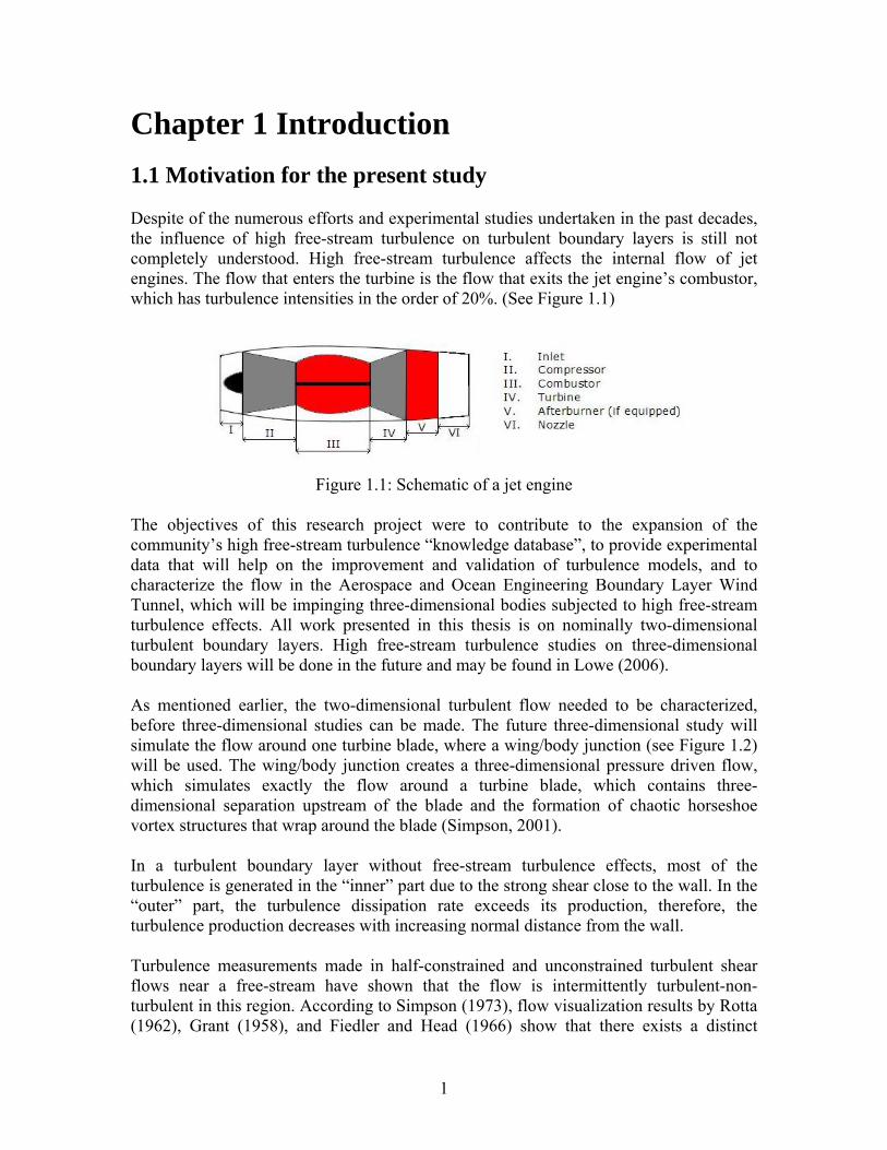
Chapter 1 Introduction 1.1 Motivation for the present study Despite of the numerous efforts and experimental studies undertaken in the past decades, the influence of high free-stream turbulence on turbulent boundary layers is still not completely understood. High free-stream turbulence affects the internal flow of jet engines. The flow that enters the turbine is the flow that exits the jet engine’s combustor, which has turbulence intensities in the order of 20%. (See Figure 1.1)

Figure 1.1: Schematic of a jet engine

The objectives of this research project were to contribute to the expansion of the community’s high free-stream turbulence “knowledge database”, to provide experimental data that will help on the improvement and validation of turbulence models, and to characterize the flow in the Aerospace and Ocean Engineering Boundary Layer Wind Tunnel, which will be impinging three-dimensional bodies subjected to high free-stream turbulence effects. All work presented in this thesis is on nominally two-dimensional turbulent boundary layers. High free-stream turbulence studies on three-dimensional boundary layers will be done in the future and may be found in Lowe (2006). As mentioned earlier, the two-dimensional turbulent flow needed to be characterized, before three-dimensional studies can be made. The future three-dimensional study will simulate the flow around one turbine blade, where a wing/body junction (see Figure 1.2) will be used. The wing/body junction creates a three-dimensional pressure driven flow, which simulates exactly the flow around a turbine blade, which contains three-dimensional separation upstream of the blade and the formation of chaotic horseshoe vortex structures that wrap around the blade (Simpson, 2001).

In a turbulent boundary layer without free-stream turbulence effects, most of the turbulence is generated in the “inner” part due to the strong shear close to the wall. In the “outer” part, the turbulence dissipation rate exceeds its production, therefore, the turbulence production decreases with increasing normal distance from the wall. Turbulence measurements made in half-constrained and unconstrained turbulent shear flows near a free-stream have shown that the flow is intermittently turbulent-non-turbulent in this region. According to Simpson (1973), flow visualization results by Rotta (1962), Grant (1958), and Fiedler and Head (1966) show that there exists a distinct

1

boundary between the turbulent fluid and non-turbulent fluid, called the “viscous superlayer”, which has an irregular, time-dependent shape with a very large interfacial area.

Figure 1.2: Wing/body junction (simulating a turbine blade) [Simpson 2001, modified]

Non-turbulent fluid is converted to turbulent fluid as the shear layer moves downstream. The conversion process is called entrainment. Flow instabilities cause depressions on the viscous superlayer. These depressions grow to large amplitudes and rapidly move into the surrounding non-turbulent fluid. The rapidly moving fluid composed of three-dimensional bulges of size or scale of the shear layer thickness, rolls up and surrounds some of the non-turbulent fluid. The surrounding process is called engulfment. The engulfed non-turbulent fluid is convected with the shear layer. At the viscous superlayer, viscous mixing occurs, transmitting vorticity to the engulfed fluid, and therefore causing it to become turbulent. The flow near the free-stream boundary is then characterized by irrotational fluid trapped between the three-dimensional bulges of turbulent fluid.

Figure 1.3: Engulfment process (After drawing of Simpson (1973)) In a turbulent boundary layer with free-stream turbulence effects, there exists the possibility of energy transport from the free-stream to the turbulent boundary layer. Several authors have shown in previous studies that free-stream turbulence increases the

2

skin friction and that implies that the turbulence production increases. The integral length scale of the free-stream turbulence also affects the boundary layer. Increasing the free-stream turbulent intensity may cause the lengthscale to penetrate deeper into the boundary layer. Small free-stream fluctuations do not strongly influence the turbulent-non-turbulent interface or boundary, while large free-stream fluctuations produce a series of waves or wavelike segments that influence the turbulent flow beneath. According to Cousteix and Houdeville (1988) “long wavelength unsteady free-stream fluctuations have almost no effect on the boundary layer beneath, as long as the flow is not near separation with strong adverse pressure gradients.” In addition, this condition is reflected in long streamwise integral length scales. As it is known, the free-stream turbulence and the boundary layer turbulence generated near the wall are not coherent and are at different streamwise wavelengths, therefore there can only be very small interaction and effect on the Reynolds-averaged ergodic statistics. Based on the nature of the turbulent-non-turbulent interface and on the entrainment process, it is expected that only the high free-stream turbulence intensities with comparable wavelengths to those being produced by the boundary layer will show non-linear interactions and affect the Reynolds-averaged behavior. For the first time, due to the technology available for this experiment, the skin friction coefficient (Cf) was deduced from the viscous sublayer, whereas in most of the previous published studies the authors assumed a semi-log layer with low free-stream turbulence constants to obtain the skin friction. 1.2 Previous free-stream turbulence studies Hancock and Bradshaw (1983) made mean flow and turbulence measurements in an incompressible two-dimensional turbulent boundary layer at constant pressure (zero pressure gradient). The free-stream turbulence (4% intensity) was nearly homogeneous and nearly isotropic, and was generated by square-mesh/square-bar biplane grids. Boundary layer measurements were made on a 15-mm thick flat plate which was 2.4 m long and was positioned half way between the tunnel’s ceiling and floor. In order to reduce fluctuating separations the plate’s leading edge was ogive-shaped. Skin-friction measurements were obtained from pitot-tube velocity profile measurements in the log region using the assumption that the log law is valid under free-stream turbulence conditions. The flow’s two-dimensionality was checked by using Preston tubes that were positioned at the plate’s centerline. Based on their measurements, Hancock and Bradshaw concluded that the velocity approaches the free-stream value slowly when the free-stream turbulence intensity is high. The shear stress approaches zero outside the boundary layer while the three mean square intensities or normal stresses become almost equal. They also concluded that the free-stream length scale has a large effect on the boundary layer’s response and that there is a nonlinear relationship between the effects of free-stream turbulence and the free-stream turbulence intensity.

3

Hancock and Bradshaw also defined two parameters: the dissipation length parameter

( ), which is based on the decaying isotropic turbulence, ueL u

e

eee L

udxud

U2/322 )()( −

= , where

x is the distance from the turbulence generator grid and the free-stream turbulence parameter (β) that combines the dependence of the skin friction on the turbulence

intensity and dissipation length scale, 2

'

5.99

+

⎟⎠⎞

⎜⎝⎛

≡

δ

β ue

e

LUu

, where eU

u⎟⎠⎞

⎜⎝⎛ ' is the turbulence

intensity. Hancock and Bradshaw (1989) made new measurements for a wide variety of length-scales in a turbulent boundary layer also on a flat plate with zero pressure gradient. Nearly isotropic free-stream turbulence was generated by a grid, as in the studies from 1983. In that study the authors used conditional sampling techniques with the flat-plate boundary layer heated near the leading edge to set apart the free-stream fluid from the boundary-layer fluid. The velocity fluctuations (u, v, w) and their spectra were measured in the free-stream. Pitot tubes were used to measure mean velocities and the skin-friction coefficients were obtained from semi-log plots assuming that the semi-log law of the wall mean velocity profile remains valid under free-stream turbulence conditions. Velocity fluctuation measurements were made by using crossed hot-wire anemometers while temperature fluctuation measurements were made with a single wire operated at constant current. Based on the measurements published in 1989, Hancock and Bradshaw concluded that near the wall there was an increased loss of turbulent kinetic energy by diffusion, larger free-stream length-scales infiltrate further into the boundary layer. Based on the turbulent kinetic energy and shear-stress balances, they noticed that the free-stream turbulence has no effect on the dissipation length parameter. Based on the fact that the dissipation length parameter is not affected by the free-stream turbulence, the authors also concluded that the shear stress provides a more meaningful velocity scale for the boundary layer turbulence instead of the turbulence intensity. Blair (1983ab) made mean flow and turbulence measurements in a two-dimensional boundary layer at zero pressure gradient. The turbulence was generated by square-mesh/square-bar biplane grids and the turbulence intensity varied from 0.25% to 7%. Changes in the wall skin friction were obtained from wake depression measurements

using Bradshaw’s equation: 22

11)(41 00

tanRe0

0ff

f

f CCC

C

tcons⎟⎟

⎠

⎞

⎜⎜

⎝

⎛−Π−Π−=

=κκ

δ

.

Blair pointed out by experimental data comparison that Hancock’s and Bradshaw’s free-stream turbulence parameter (β) only worked correctly for high Reθ. The β-parameter

4

over predicted the changes in skin friction at lower Reθ. Blair introduced a new parameter named Hancock-Bradshaw-Blair (HBB), which is a function of Reθ, turbulence intensity,

and dissipation length scale:

⎟⎟⎠

⎞⎜⎜⎝

⎛⎟⎠⎞

⎜⎝⎛ −

+⎟⎟⎠

⎞⎜⎜⎝

⎛+

⎟⎠⎞

⎜⎝⎛

=

400Re

exp312

(%)'

5.99

θ

δ

ue

e

LUu

HBB . He also stated that

the skin friction increased due to the higher levels of turbulence and that the semi-log region of the mean velocity profile was relatively unaffected by changes in the free-stream turbulence level. Hollingsworth and Bourgogne (1995) conducted a study to document the response of a turbulent boundary layer to a flow with high free-stream and approximately streamwise-uniform levels of turbulent intensity. Measurements were taken in a two-dimensional turbulent boundary layer beneath a free-stream produced by a two-stream mixing layer. The flat plate used in the experiment was positioned downstream of a splitter wall used to form the mixing layer, and the gradient direction of the mixing layer was parallel to the boundary layer’s span. Measurements of mean and fluctuating velocities were taken by using hot-wires and the data were taken for free-stream turbulence intensities in the order of up to 16%. The authors state that previous studies investigated the effects of free-stream turbulent intensities below 10%, and free-stream turbulence was nearly isotropic and generated by passive grids that create relatively low intensity and decays quickly as it convects downstream. Turbulence generated by other means, such as mixing two flows together, as shown in this paper by Hollingsworth and Bourgogne, generate higher turbulence intensities, as high as 20%, that have a longer life. Uτ was determined using two different approaches. The mean velocity profiles were fit from y+ = 30 to y+ = 70 to the semi-log law of the wall using the Coles constants (κ = 0.41 and C = 5). The resulting Uτ from the law of the wall was compared to a Uτ obtained from a linear fit to the data for y+ ≤ 5. According to the authors those two Uτ values agreed to within ±2%. From their experiments, the authors concluded that an excess in stream-wise momentum was formed in and above the outer region of the boundary layer due to an interaction between the vorticity fields of the boundary layer and the mixing layer. They also concluded that the skin-friction increased by up to 73% compared to the expected values based on the streamwise development length of the boundary layer. During the experiments the authors were not successful with the free-stream turbulence decay. For some reason, the turbulence level did not decay and the free-stream flow had a complex structure producing three-dimensional effects on the boundary layer. Thole and Bogard (1996) studied the effect of high free-stream turbulence on a flat plate using an active turbulence generator. Their study contains experimental data of mean and rms velocities, velocity correlation coefficients, length scales and power spectra for a turbulent boundary layer subjected to high free-stream turbulence up to an intensity of 20%. The active generator was designed by the authors and consisted of a row of small, high velocity, normal jets injecting air into the cross-flow mainstream. The mean and rms velocities, and the uv correlation were obtained by using a two-component LDV system with frequency shifting. Skin friction was estimated from the constant stress part of the

5

log layer (-uv = Uτ2). Integral time scales and power spectra were obtained by using hot-

wire measurements of the streamwise velocity fluctuations. A spectrum analyzer was used to obtain the power spectra. The integral time scales were directly calculated from correlations of the digitized hot-wire measurements or from the power spectra extrapolated to zero frequency. Integral length scales were determined from the measured integral time scales and mean velocities by using Taylor’s hypothesis that the turbulence convection speed was U. Based on the results of their experiments, Thole and Bogard made several conclusions. They concluded that the mean velocity profile retained the semi-log law near the wall for all levels of free-stream turbulence tested, but the outer region of the profile had some significant alterations. The direct measurements of total shear stress proved that the log law is valid for the flows under high free-stream turbulence. The authors observed that the high free-stream turbulence caused the outer part of the boundary layer to become much flatter. In addition, the free-stream turbulent eddies penetrate into the boundary layer at high free-stream turbulence levels, and that is proven by the measured lengthscale and spectra. The velocity spectra were much broader than for the low free-stream turbulence boundary layer and that is due to much larger lengthscales for the free-stream turbulence. Finally, due to the uncorrelated nature of the free-stream turbulence and the boundary layer generated turbulence, the Ruv correlation coefficient throughout the boundary layer was reduced. Stefes and Fernholz (2004) measured mean and fluctuating velocity profiles and the skin friction in an axisymmetric turbulent boundary layer with zero pressure gradient and free-stream turbulence intensities ranging from 1% to 13%. The ratio of the u-component streamwise integral lengthscale in the free-stream and the boundary layer thickness varied between 0.5 and 2 in the streamwise direction. The high free-stream turbulence intensities were generated by jets injected normal to the flow. Measurements of mean and fluctuating velocities were made by using a miniature single and x-wire probes. Skin friction measurements were made by using Preston tubes, wall hot-wires and oil-film interferometry. Under free-stream turbulence conditions the authors observed that the skin friction increased by approximately 34%. The measured fractional increase in skin friction correlated well with the Hancock-Bradshaw-Blair parameter. Stefes and Fernholz state that the skin friction increase is due to the increased mixing by the free-stream turbulence that penetrates into the boundary layer and which thereby reduces the mean velocity gradient in the outer region, resulting in a fuller profile. The authors observed that the mean velocity profile agrees with the linear-law and that the semi-log law in the inner region of the boundary layer is independent of the free-stream turbulent intensity. Other observations include the fact that the free-stream turbulence affects the wake parameter and the mean velocity distribution in the outer layer significantly. Stefes and Fernholz concluded that the distribution of the mean velocity is affected in a similar way as by a mild favorable pressure gradient. They also observed that the distributions of

Reynolds normal stress components, 2

2'

τuu , plotted in inner-law scaling, collapsed on top of

each other in the viscous sublayer and in the lower part of the of the buffer layer, but an

6

increase in their peak values by approximately 25% at a turbulence intensity of 13% was observed when compared to the data at a turbulence intensity of 1%. By increasing the free-stream turbulence, the Reynolds shear stress profiles extended further out into the boundary layer’s outer region without causing a higher production of Reynolds normal stresses. Finally, the authors observed that free-stream turbulence barely affects the production in the inner layer. Liu and Pletcher (2005) calculated turbulent boundary layers with free-stream turbulence by using Large Eddy Simulation (LES). The turbulent boundary layers were subjected to free-stream turbulent intensities of 0%, 5% and 7.5%. The authors investigated the influence of free-stream turbulence length scale and intensity on the skin friction, mean velocity, and rms profiles. Their numerical results verified that as the free-stream turbulent intensity increased, the log region extended and the size of the wake component decreased. The same results were observed by Hancock and Bradshaw on their experiments. According to Liu and Pletcher the rms velocities increased with increasing free-stream turbulence level. Also the skin-friction coefficient increased with the free-stream turbulence level increase. The authors stated that their results agreed well with the experimentally based correlation of Hancock and Bradshaw. Just for comparison purposes the data of Liu and Pletcher (2005) was plotted with Stefes and Fernholz (2004) data and is shown in Figure 3.97. 1.3 Counterflow jet and coflow jet characterization In order to study the wing/body junction flow under high free-stream turbulence, an active turbulence generator capable of generating high turbulence intensity had to be designed and built. The turbulence generator design was based on a previous design by Bangert, Kohli, Sauer and Thole (1997). Design details about the turbulence generator can be found in Chapter 2. The generator creates high free-stream turbulence in a wind-tunnel by injecting air parallel to the flow in two directions. There are 42 jets opposing the wind tunnel flow and 42 jets in the direction of the flow. Jets in a counterflow and jets in a coflow have been studied by several authors with the intent to characterize such flows. As it was observed by Bernero (2000a) and Yoda et al. (1996), jets in a counterflow behave differently depending on the velocity ratio between the jet and the counterflow. It has been shown by them that for velocity ratios (Vr, jet orifice velocity to counterflow velocity) smaller than 3.4 the jet has a stable and unstable phase. For velocity ratios equal or greater than 3.4 the jet has only an unstable phase. The jet is in the stable phase when it is characterized by a single and symmetric vortex ring, and it reaches the unstable phase as the jet’s penetration length increases. Due to the counterflow perturbations, the jet becomes asymmetric and flapping occurs. Yoda et. al. (1996) showed that for velocity ratios greater or equal to 2.2, the jet’s penetration length can be determined by the following model: ))()(8.2( rp VDx = , where xp is the penetration length in centimeters, D is the jet’s diameter in centimeters and Vr is the velocity ratio.

7

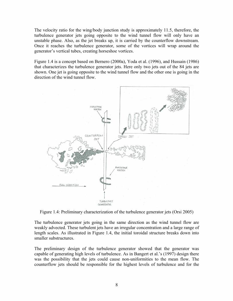
The velocity ratio for the wing/body junction study is approximately 11.5, therefore, the turbulence generator jets going opposite to the wind tunnel flow will only have an unstable phase. Also, as the jet breaks up, it is carried by the counterflow downstream. Once it reaches the turbulence generator, some of the vortices will wrap around the generator’s vertical tubes, creating horseshoe vortices. Figure 1.4 is a concept based on Bernero (2000a), Yoda et al. (1996), and Hussain (1986) that characterizes the turbulence generator jets. Here only two jets out of the 84 jets are shown. One jet is going opposite to the wind tunnel flow and the other one is going in the direction of the wind tunnel flow.

Figure 1.4: Preliminary characterization of the turbulence generator jets (Orsi 2005)

The turbulence generator jets going in the same direction as the wind tunnel flow are weakly advected. These turbulent jets have an irregular concentration and a large range of length scales. As illustrated in Figure 1.4, the initial toroidal structure breaks down into smaller substructures. The preliminary design of the turbulence generator showed that the generator was capable of generating high levels of turbulence. As in Bangert et al.’s (1997) design there was the possibility that the jets could cause non-uniformities to the mean flow. The counterflow jets should be responsible for the highest levels of turbulence and for the

8

highest flow non-uniformities, if flow non-uniformities are present. Detailed characterization of the turbulence generator’s flow can be found in Chapter 3. 1.4 Organization of thesis The remainder of this thesis is organized in three more chapters. Chapter 2 describes the apparatus and instrumentation used for the experiments. It includes a detailed description of the turbulence generator, a brief description of the seven-hole pressure probe system used to make flowfield measurements, and an explanation of how the Third Generation Comprehensive Laser Doppler Velocimeter system was used in this experiment in order to make particle velocity measurements. Chapter 3 contains the results and discussions about the experiments, including Schlieren pictures of the turbulence generator jets, plane measurements using the seven-hole pressure probe, and mean and fluctuating velocity measurements of two-dimensional turbulent boundary layers. Chapter 4 has the conclusions about the present experiments and previous experiments conducted by other authors.

9

Chapter 2 Apparatus and Instrumentation 2.1 Boundary Layer Wind Tunnel Measurements were taken in the Aerospace and Ocean Engineering (AOE) open-circuit low-speed boundary layer wind tunnel. This experimental facility has been used for several decades where data were collected and results published in referred journals (i.e. Devenport et al. (1990), Ölçmen (1995), and Simpson (2001)). Other information about this facility is available online at http://www.aoe.vt.edu/research/facilities/ bllab.php. The wind tunnel is powered by a 19 kW centrifugal blower and its speed is controlled by a fixed-setting damper. Before the intake air reaches the test section, it passes through a plenum, a section of honeycomb that is used to remove the flow’s mean swirl, and seven wire-mesh screens used to reduce the turbulence intensity. The air also passes through a 4:1 contraction that is used to reduce turbulence levels and accelerate the flow, is subjected to another 1.5:1 contraction with a throat height of 0.251 m (0.823 ft) over the first 5.35 ft of the test section. The wind tunnel has a 0.91 m (3 ft) wide by 7.3 m (24 ft) long rectangular cross-section with a variable flat-ceiling height. The free-stream velocity and the free-stream temperature are measured 1.63 m (5.35 ft) downstream of the test section’s entrance. At a free-stream speed of 27.5 m/sec and a free-stream temperature of 25oC, it was experimentally determined that the airflow entering the test section has a uniform potential core within 0.5% in the spanwise direction and 1% in the vertical direction. The turbulence intensity in the freestream was determined to be 0.1%.

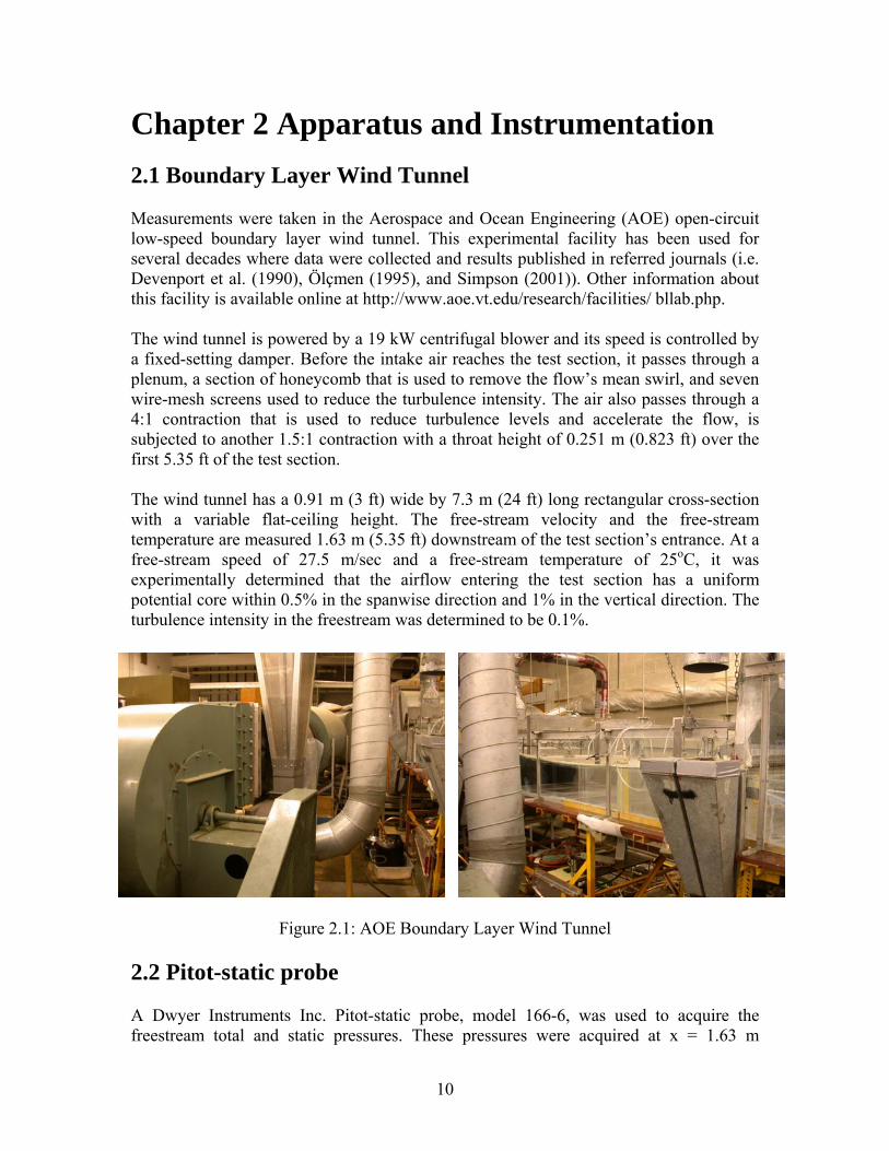
Figure 2.1: AOE Boundary Layer Wind Tunnel

2.2 Pitot-static probe A Dwyer Instruments Inc. Pitot-static probe, model 166-6, was used to acquire the freestream total and static pressures. These pressures were acquired at x = 1.63 m

10

downstream of the test section’s entrance, y = 14 cm and z = 31.75 cm. The static ports have a diameter of 0.0381 cm and the total pressure port has a diameter of 0.140 cm.

2.3 Inclined manometer A Dwyer Instruments Inc. inclined manometer, model 246, with a measuring range between 0 and 6 inches of water and with a minor scale division of 0.02 inches of water, was used to measure the dynamic pressure in the freestream. Uncertainty of ±0.01 inches of water.

2.4 Thermometer An H-B Instrument Co. mercury thermometer with a measuring range between 8oC and 42oC and with a minor scale division of 1oC, was used to measure the freestream temperature. Uncertainty of ±0.5 oC.

2.5 Turbulence generator The active turbulence generator was designed by Graf (2003) and built to create high free-stream turbulence in the boundary layer wind-tunnel. A turbulence intensity of 20% was desired to simulate the flow around a gas turbine compressor blade where the turbulence levels are generally on the order of 20%. The turbulence generator design was based on a previous design by Bangert, Kohli, Sauer and Thole (1997). The generator is made of steel, weighs 14 Kg, and is located 5.08 cm away from the left and right tunnel walls, refer to Figure 2.2. The generator’s manifold has a diameter of 7.62 cm and is 88.9 cm long. The air supply is connected to a 2.54-cm diameter valve which is attached to the top of the manifold. Six 1.27-cm diameter circular tubes are screwed to the bottom of the manifold. The tubes are 16.2 cm apart and each tube has fourteen (7 in the upstream direction and 7 in the downstream direction) 0.15-cm diameter holes, which are spaced vertically 3.18 cm apart; see Figure 2.3. The bottom of the vertical tubes are secured by a thin metal plate, which has a width of 12.2 cm and had its upstream and downstream edges smoothed and angled to reduce any disturbances to the flow that passes over it. And the top of the vertical tubes are secured by another metal plate, which is located outside of the test section, attached to the ceiling. These metal plates keep the generator fixed in place to avoid any movement during the experiments. Compressed air is fed to the turbulence generator by a 2.54-cm diameter steel pipe (“air line”) that is connected to the two air tanks that feed air to the Virginia Tech Supersonic Wind Tunnel. The tanks are initially charged to 1.79 MPa (260 psi) and the air passes through a pressure regulator (Fisher Regulator, Serial/Model 627H-97, type 627H, Range: 240-500 psig) which drops the pressure from 1.79 MPa (260 psi) to 689 kPa (100 psi), setting the generator’s manifold pressure to 689 kPa (100 psi); See Chapter 3, section 3.4 for details about why 689 kPa was the pressure chosen. A pressure gage (Ashcroft commercial pressure gage, 0-600 psi, 10-psi increments, type 1005P, ASME B

11

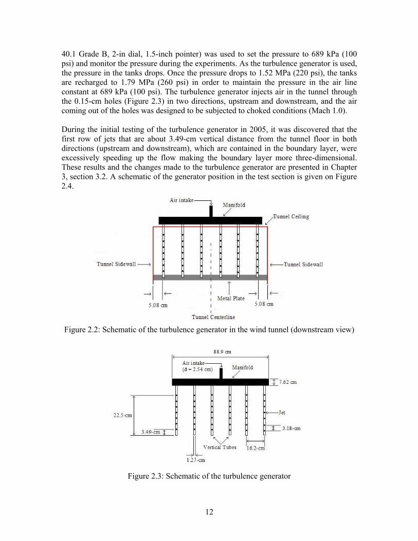
40.1 Grade B, 2-in dial, 1.5-inch pointer) was used to set the pressure to 689 kPa (100 psi) and monitor the pressure during the experiments. As the turbulence generator is used, the pressure in the tanks drops. Once the pressure drops to 1.52 MPa (220 psi), the tanks are recharged to 1.79 MPa (260 psi) in order to maintain the pressure in the air line constant at 689 kPa (100 psi). The turbulence generator injects air in the tunnel through the 0.15-cm holes (Figure 2.3) in two directions, upstream and downstream, and the air coming out of the holes was designed to be subjected to choked conditions (Mach 1.0). During the initial testing of the turbulence generator in 2005, it was discovered that the first row of jets that are about 3.49-cm vertical distance from the tunnel floor in both directions (upstream and downstream), which are contained in the boundary layer, were excessively speeding up the flow making the boundary layer more three-dimensional. These results and the changes made to the turbulence generator are presented in Chapter 3, section 3.2. A schematic of the generator position in the test section is given on Figure 2.4.

Figure 2.2: Schematic of the turbulence generator in the wind tunnel (downstream view)

Figure 2.3: Schematic of the turbulence generator

12

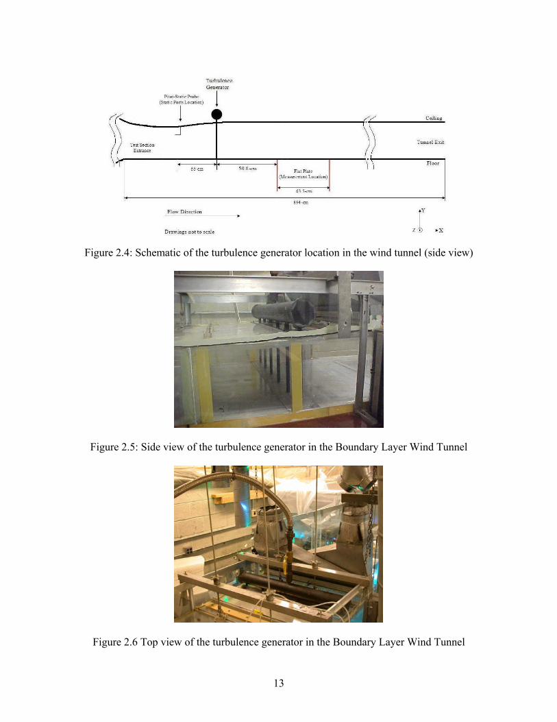
Figure 2.4: Schematic of the turbulence generator location in the wind tunnel (side view)

Figure 2.5: Side view of the turbulence generator in the Boundary Layer Wind Tunnel

Figure 2.6 Top view of the turbulence generator in the Boundary Layer Wind Tunnel

13

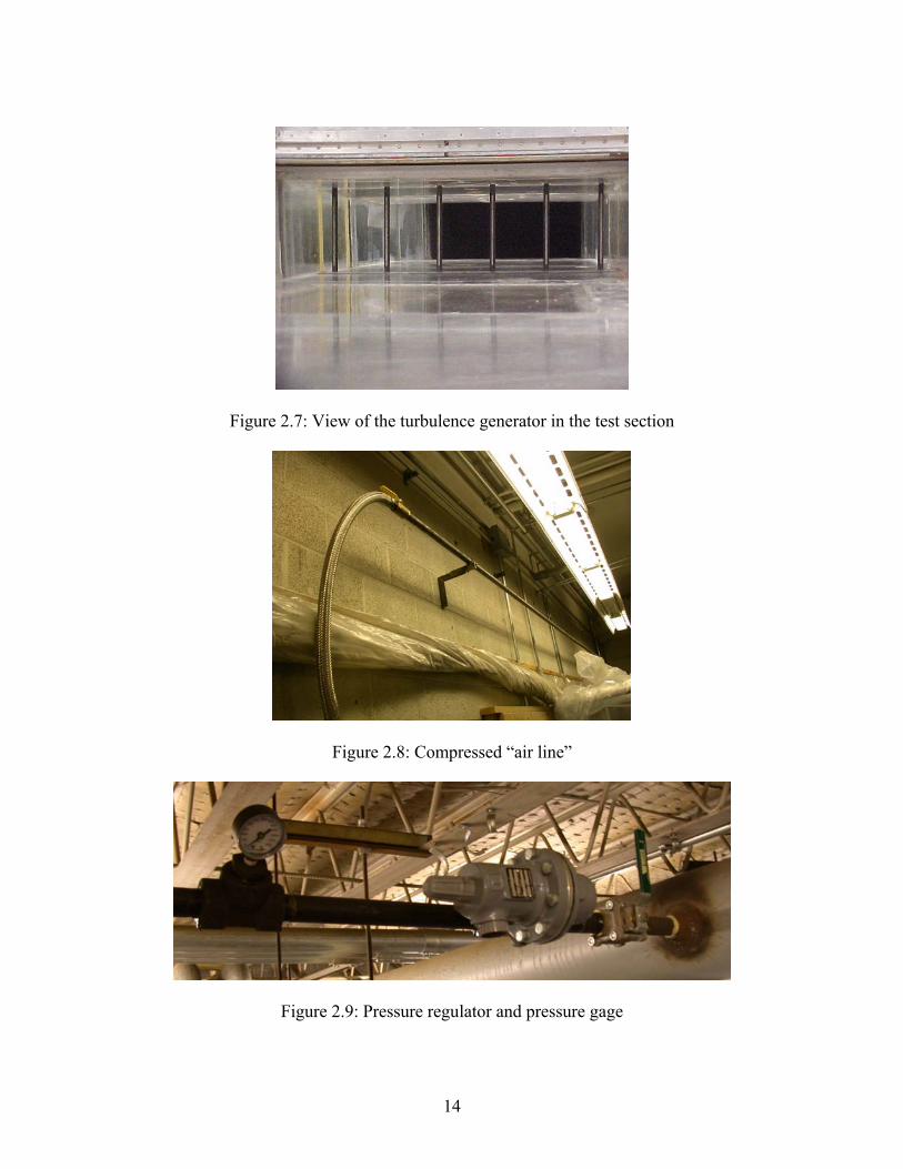
Figure 2.7: View of the turbulence generator in the test section

Figure 2.8: Compressed “air line”

Figure 2.9: Pressure regulator and pressure gage

14

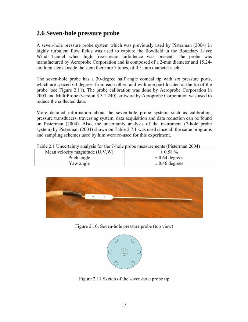
2.6 Seven-hole pressure probe A seven-hole pressure probe system which was previously used by Pisterman (2004) in highly turbulent flow fields was used to capture the flowfield in the Boundary Layer Wind Tunnel when high free-stream turbulence was present. The probe was manufactured by Aeroprobe Corporation and is composed of a 2-mm diameter and 15.24-cm long stem. Inside the stem there are 7 tubes, of 0.5-mm diameter each. The seven-hole probe has a 30-degree half angle conical tip with six pressure ports, which are spaced 60-degrees from each other, and with one port located at the tip of the probe (see Figure 2.11). The probe calibration was done by Aeroprobe Corporation in 2003 and MultiProbe (version 3.3.1.240) software by Aeroprobe Corporation was used to reduce the collected data. More detailed information about the seven-hole probe system, such as calibration, pressure transducers, traversing system, data acquisition and data reduction can be found on Pisterman (2004). Also, the uncertainty analysis of the instrument (7-hole probe system) by Pisterman (2004) shown on Table 2.7.1 was used since all the same programs and sampling schemes used by him were re-used for this experiment. Table 2.1 Uncertainty analysis for the 7-hole probe measurements (Pisterman 2004)

Mean velocity magnitude (U,V,W) ± 0.58 % Pitch angle ± 0.64 degrees Yaw angle ± 0.46 degrees

Figure 2.10: Seven-hole pressure probe (top view)

Figure 2.11 Sketch of the seven-hole probe tip

15

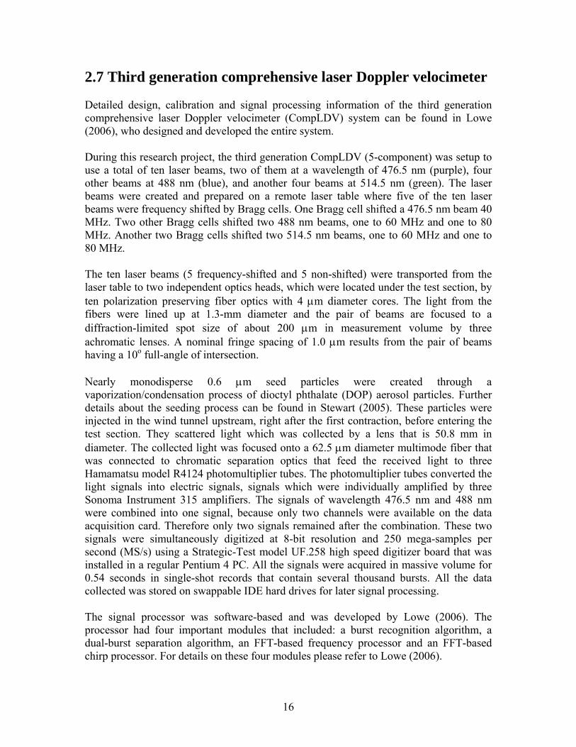
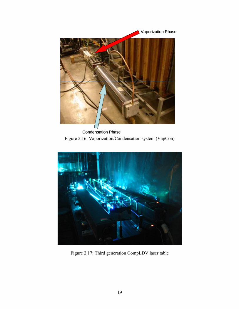
2.7 Third generation comprehensive laser Doppler velocimeter Detailed design, calibration and signal processing information of the third generation comprehensive laser Doppler velocimeter (CompLDV) system can be found in Lowe (2006), who designed and developed the entire system. During this research project, the third generation CompLDV (5-component) was setup to use a total of ten laser beams, two of them at a wavelength of 476.5 nm (purple), four other beams at 488 nm (blue), and another four beams at 514.5 nm (green). The laser beams were created and prepared on a remote laser table where five of the ten laser beams were frequency shifted by Bragg cells. One Bragg cell shifted a 476.5 nm beam 40 MHz. Two other Bragg cells shifted two 488 nm beams, one to 60 MHz and one to 80 MHz. Another two Bragg cells shifted two 514.5 nm beams, one to 60 MHz and one to 80 MHz. The ten laser beams (5 frequency-shifted and 5 non-shifted) were transported from the laser table to two independent optics heads, which were located under the test section, by ten polarization preserving fiber optics with 4 µm diameter cores. The light from the fibers were lined up at 1.3-mm diameter and the pair of beams are focused to a diffraction-limited spot size of about 200 µm in measurement volume by three achromatic lenses. A nominal fringe spacing of 1.0 µm results from the pair of beams having a 10o full-angle of intersection. Nearly monodisperse 0.6 µm seed particles were created through a vaporization/condensation process of dioctyl phthalate (DOP) aerosol particles. Further details about the seeding process can be found in Stewart (2005). These particles were injected in the wind tunnel upstream, right after the first contraction, before entering the test section. They scattered light which was collected by a lens that is 50.8 mm in diameter. The collected light was focused onto a 62.5 µm diameter multimode fiber that was connected to chromatic separation optics that feed the received light to three Hamamatsu model R4124 photomultiplier tubes. The photomultiplier tubes converted the light signals into electric signals, signals which were individually amplified by three Sonoma Instrument 315 amplifiers. The signals of wavelength 476.5 nm and 488 nm were combined into one signal, because only two channels were available on the data acquisition card. Therefore only two signals remained after the combination. These two signals were simultaneously digitized at 8-bit resolution and 250 mega-samples per second (MS/s) using a Strategic-Test model UF.258 high speed digitizer board that was installed in a regular Pentium 4 PC. All the signals were acquired in massive volume for 0.54 seconds in single-shot records that contain several thousand bursts. All the data collected was stored on swappable IDE hard drives for later signal processing. The signal processor was software-based and was developed by Lowe (2006). The processor had four important modules that included: a burst recognition algorithm, a dual-burst separation algorithm, an FFT-based frequency processor and an FFT-based chirp processor. For details on these four modules please refer to Lowe (2006).

16

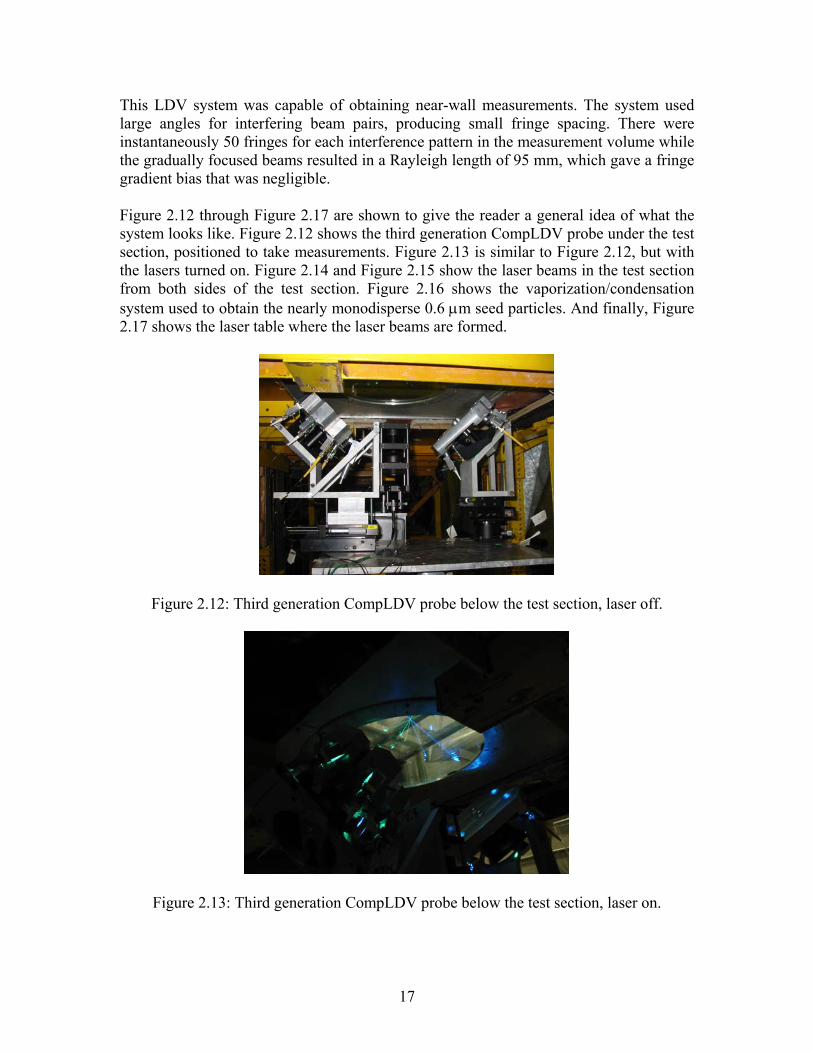
This LDV system was capable of obtaining near-wall measurements. The system used large angles for interfering beam pairs, producing small fringe spacing. There were instantaneously 50 fringes for each interference pattern in the measurement volume while the gradually focused beams resulted in a Rayleigh length of 95 mm, which gave a fringe gradient bias that was negligible. Figure 2.12 through Figure 2.17 are shown to give the reader a general idea of what the system looks like. Figure 2.12 shows the third generation CompLDV probe under the test section, positioned to take measurements. Figure 2.13 is similar to Figure 2.12, but with the lasers turned on. Figure 2.14 and Figure 2.15 show the laser beams in the test section from both sides of the test section. Figure 2.16 shows the vaporization/condensation system used to obtain the nearly monodisperse 0.6 µm seed particles. And finally, Figure 2.17 shows the laser table where the laser beams are formed.

Figure 2.12: Third generation CompLDV probe below the test section, laser off.

Figure 2.13: Third generation CompLDV probe below the test section, laser on.

17

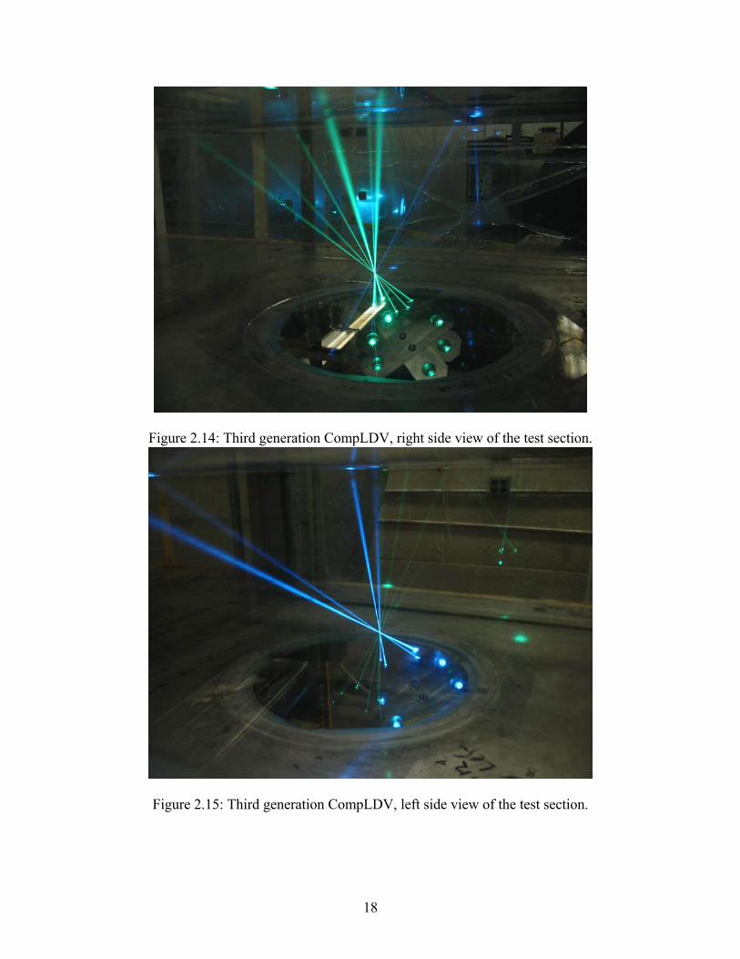
Figure 2.14: Third generation CompLDV, right side view of the test section.

Figure 2.15: Third generation CompLDV, left side view of the test section.

18

Vaporization Phase

Condensation Phase

Vaporization Phase

Condensation Phase

Figure 2.16: Vaporization/Condensation system (VapCon)

Figure 2.17: Third generation CompLDV laser table

19

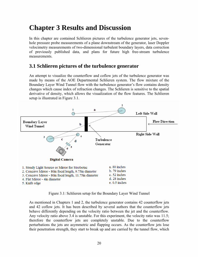
Chapter 3 Results and Discussion In this chapter are contained Schlieren pictures of the turbulence generator jets, seven-hole pressure probe measurements of a plane downstream of the generator, laser Doppler velocimetry measurements of two-dimensional turbulent boundary layers, data correction of previously published data, and plans for future high free-stream turbulence measurements. 3.1 Schlieren pictures of the turbulence generator An attempt to visualize the counterflow and coflow jets of the turbulence generator was made by means of the AOE Departmental Schlieren system. The flow mixture of the Boundary Layer Wind Tunnel flow with the turbulence generator’s flow contains density changes which cause index of refraction changes. The Schlieren is sensitive to the spatial derivative of density, which allows the visualization of the flow features. The Schlieren setup is illustrated in Figure 3.1.

Figure 3.1: Schlieren setup for the Boundary Layer Wind Tunnel

As mentioned in Chapters 1 and 2, the turbulence generator contains 42 counterflow jets and 42 coflow jets. It has been described by several authors that the counterflow jets behave differently depending on the velocity ratio between the jet and the counterflow. Any velocity ratio above 3.4 is unstable. For this experiment, the velocity ratio was 11.5; therefore the counterflow jets are completely unstable. Due to the counterflow perturbations the jets are asymmetric and flapping occurs. As the counterflow jets lose their penetration strength, they start to break up and are carried by the tunnel flow, which

20

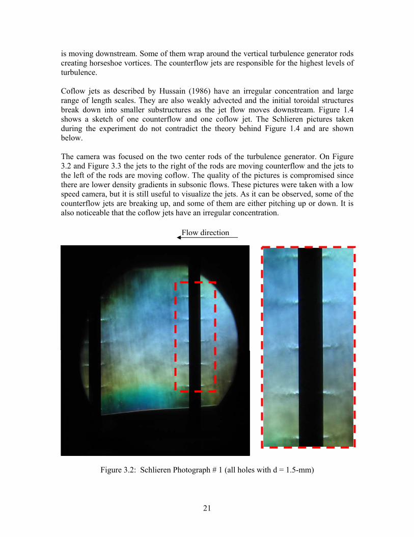
is moving downstream. Some of them wrap around the vertical turbulence generator rods creating horseshoe vortices. The counterflow jets are responsible for the highest levels of turbulence. Coflow jets as described by Hussain (1986) have an irregular concentration and large range of length scales. They are also weakly advected and the initial toroidal structures break down into smaller substructures as the jet flow moves downstream. Figure 1.4 shows a sketch of one counterflow and one coflow jet. The Schlieren pictures taken during the experiment do not contradict the theory behind Figure 1.4 and are shown below. The camera was focused on the two center rods of the turbulence generator. On Figure 3.2 and Figure 3.3 the jets to the right of the rods are moving counterflow and the jets to the left of the rods are moving coflow. The quality of the pictures is compromised since there are lower density gradients in subsonic flows. These pictures were taken with a low speed camera, but it is still useful to visualize the jets. As it can be observed, some of the counterflow jets are breaking up, and some of them are either pitching up or down. It is also noticeable that the coflow jets have an irregular concentration.

Flow direction

Figure 3.2: Schlieren Photograph # 1 (all holes with d = 1.5-mm)

21

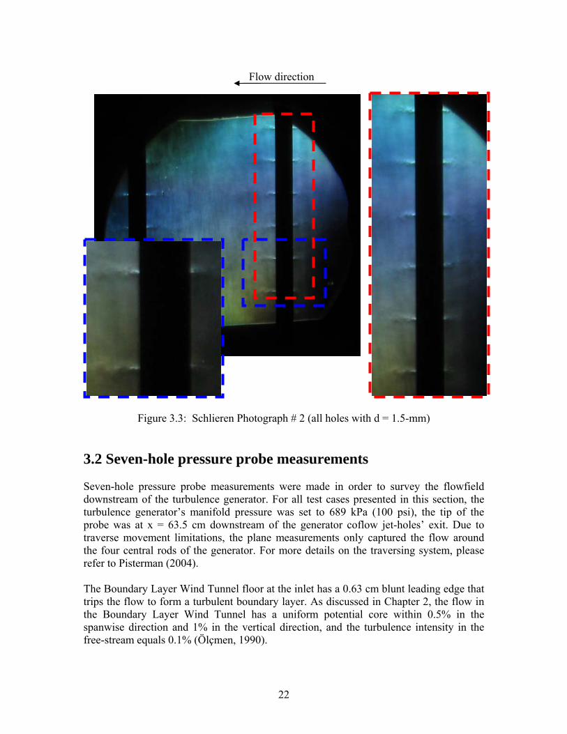
Flow direction

Figure 3.3: Schlieren Photograph # 2 (all holes with d = 1.5-mm) 3.2 Seven-hole pressure probe measurements Seven-hole pressure probe measurements were made in order to survey the flowfield downstream of the turbulence generator. For all test cases presented in this section, the turbulence generator’s manifold pressure was set to 689 kPa (100 psi), the tip of the probe was at x = 63.5 cm downstream of the generator coflow jet-holes’ exit. Due to traverse movement limitations, the plane measurements only captured the flow around the four central rods of the generator. For more details on the traversing system, please refer to Pisterman (2004). The Boundary Layer Wind Tunnel floor at the inlet has a 0.63 cm blunt leading edge that trips the flow to form a turbulent boundary layer. As discussed in Chapter 2, the flow in the Boundary Layer Wind Tunnel has a uniform potential core within 0.5% in the spanwise direction and 1% in the vertical direction, and the turbulence intensity in the free-stream equals 0.1% (Ölçmen, 1990).

22

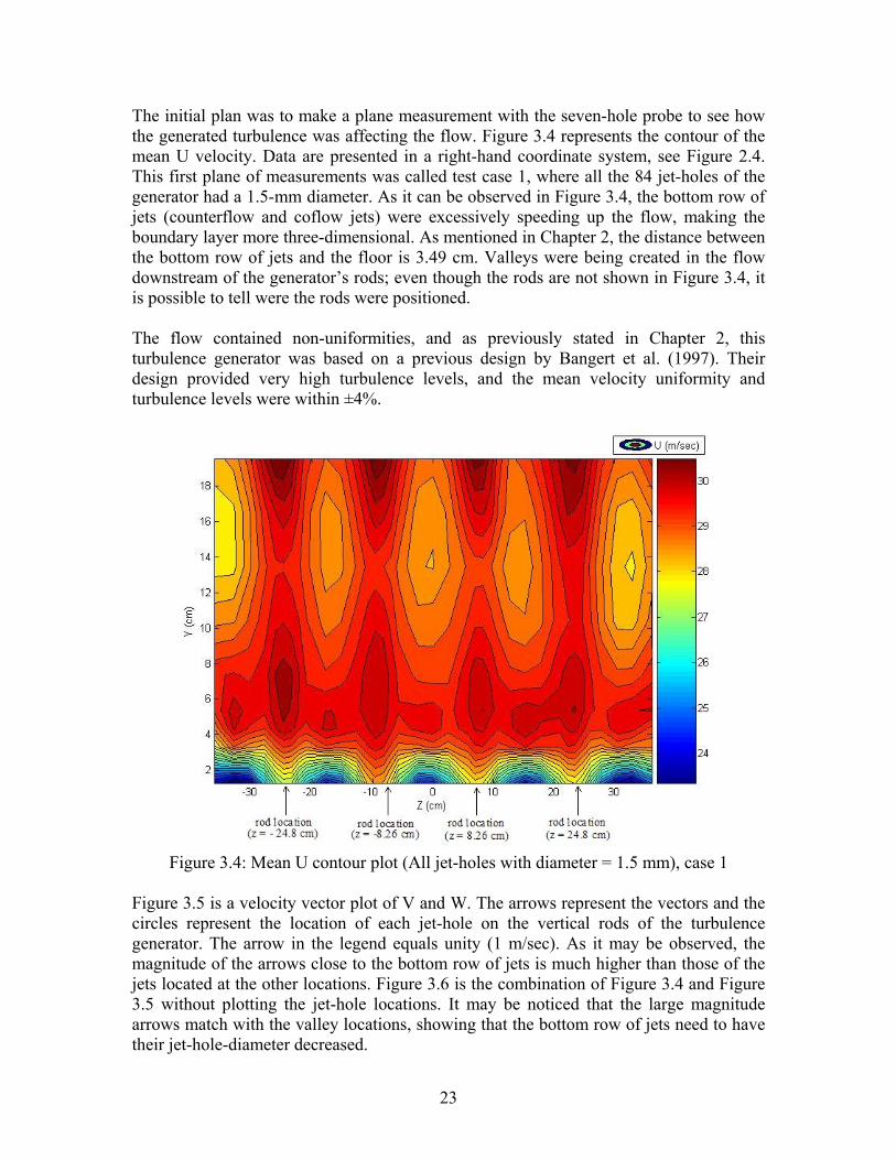
The initial plan was to make a plane measurement with the seven-hole probe to see how the generated turbulence was affecting the flow. Figure 3.4 represents the contour of the mean U velocity. Data are presented in a right-hand coordinate system, see Figure 2.4. This first plane of measurements was called test case 1, where all the 84 jet-holes of the generator had a 1.5-mm diameter. As it can be observed in Figure 3.4, the bottom row of jets (counterflow and coflow jets) were excessively speeding up the flow, making the boundary layer more three-dimensional. As mentioned in Chapter 2, the distance between the bottom row of jets and the floor is 3.49 cm. Valleys were being created in the flow downstream of the generator’s rods; even though the rods are not shown in Figure 3.4, it is possible to tell were the rods were positioned. The flow contained non-uniformities, and as previously stated in Chapter 2, this turbulence generator was based on a previous design by Bangert et al. (1997). Their design provided very high turbulence levels, and the mean velocity uniformity and turbulence levels were within ±4%.

Figure 3.4: Mean U contour plot (All jet-holes with diameter = 1.5 mm), case 1

Figure 3.5 is a velocity vector plot of V and W. The arrows represent the vectors and the circles represent the location of each jet-hole on the vertical rods of the turbulence generator. The arrow in the legend equals unity (1 m/sec). As it may be observed, the magnitude of the arrows close to the bottom row of jets is much higher than those of the jets located at the other locations. Figure 3.6 is the combination of Figure 3.4 and Figure 3.5 without plotting the jet-hole locations. It may be noticed that the large magnitude arrows match with the valley locations, showing that the bottom row of jets need to have their jet-hole-diameter decreased.

23

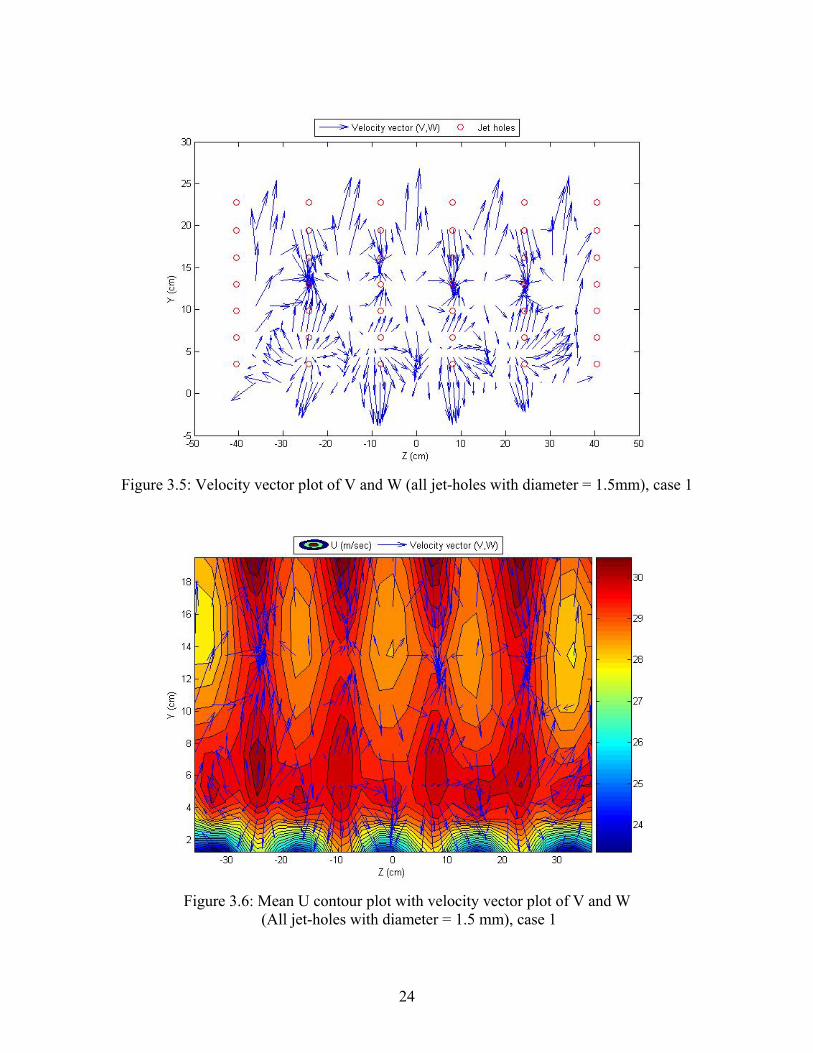
Figure 3.5: Velocity vector plot of V and W (all jet-holes with diameter = 1.5mm), case 1

Figure 3.6: Mean U contour plot with velocity vector plot of V and W

(All jet-holes with diameter = 1.5 mm), case 1

24

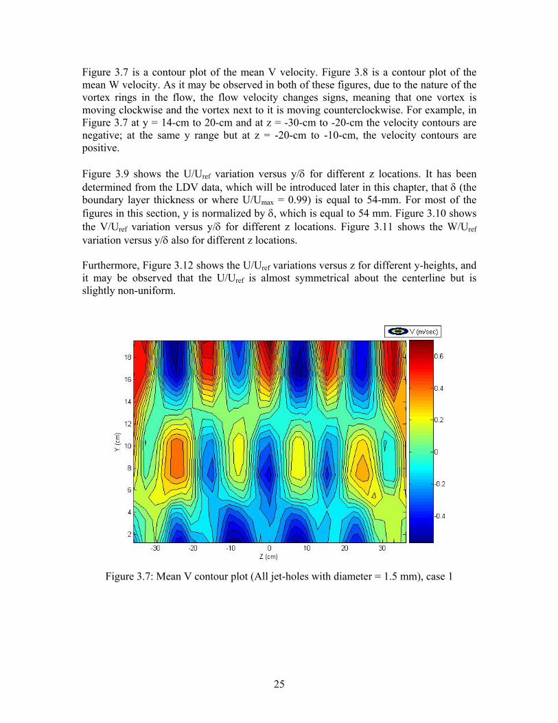
Figure 3.7 is a contour plot of the mean V velocity. Figure 3.8 is a contour plot of the mean W velocity. As it may be observed in both of these figures, due to the nature of the vortex rings in the flow, the flow velocity changes signs, meaning that one vortex is moving clockwise and the vortex next to it is moving counterclockwise. For example, in Figure 3.7 at y = 14-cm to 20-cm and at z = -30-cm to -20-cm the velocity contours are negative; at the same y range but at z = -20-cm to -10-cm, the velocity contours are positive. Figure 3.9 shows the U/Uref variation versus y/δ for different z locations. It has been determined from the LDV data, which will be introduced later in this chapter, that δ (the boundary layer thickness or where U/Umax = 0.99) is equal to 54-mm. For most of the figures in this section, y is normalized by δ, which is equal to 54 mm. Figure 3.10 shows the V/Uref variation versus y/δ for different z locations. Figure 3.11 shows the W/Uref variation versus y/δ also for different z locations. Furthermore, Figure 3.12 shows the U/Uref variations versus z for different y-heights, and it may be observed that the U/Uref is almost symmetrical about the centerline but is slightly non-uniform.

Figure 3.7: Mean V contour plot (All jet-holes with diameter = 1.5 mm), case 1

25

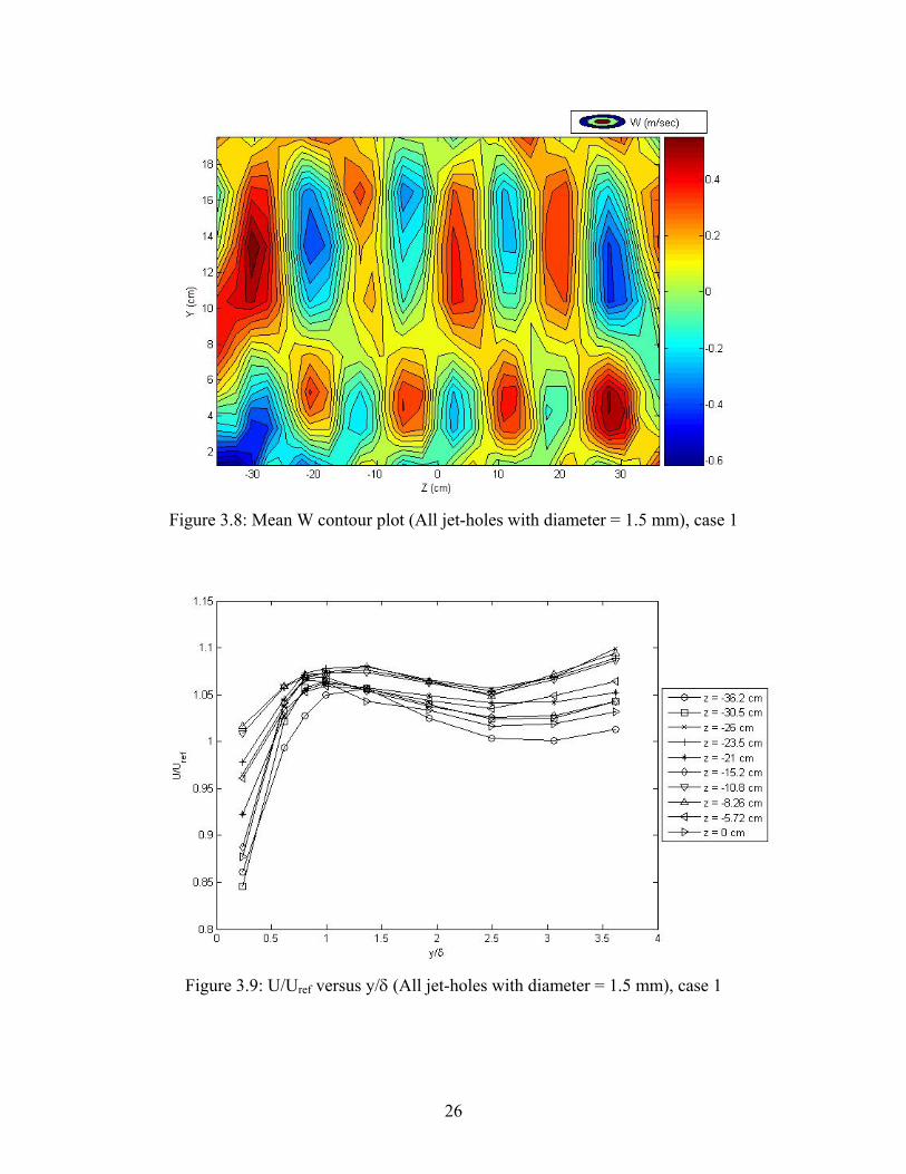
Figure 3.8: Mean W contour plot (All jet-holes with diameter = 1.5 mm), case 1

Figure 3.9: U/Uref versus y/δ (All jet-holes with diameter = 1.5 mm), case 1

26

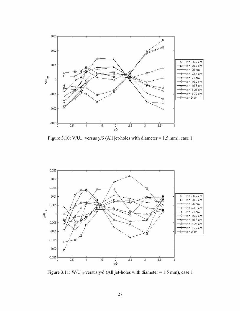
Figure 3.10: V/Uref versus y/δ (All jet-holes with diameter = 1.5 mm), case 1

Figure 3.11: W/Uref versus y/δ (All jet-holes with diameter = 1.5 mm), case 1

27

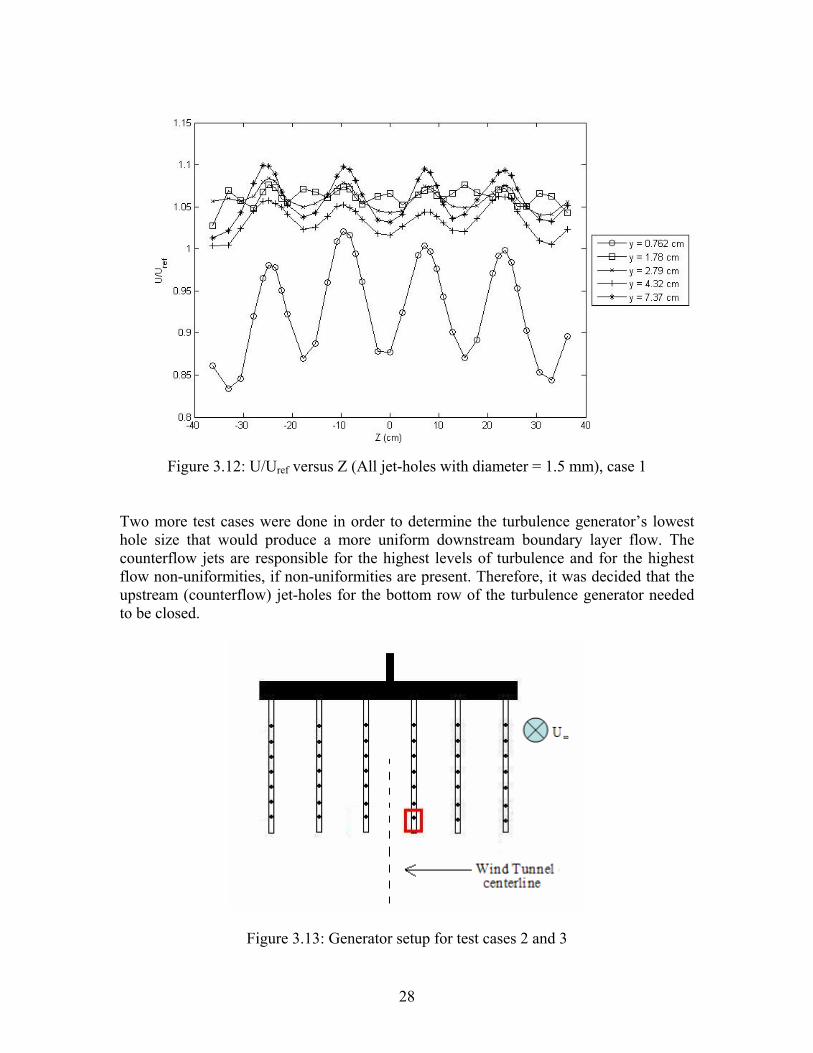
Figure 3.12: U/Uref versus Z (All jet-holes with diameter = 1.5 mm), case 1

Two more test cases were done in order to determine the turbulence generator’s lowest hole size that would produce a more uniform downstream boundary layer flow. The counterflow jets are responsible for the highest levels of turbulence and for the highest flow non-uniformities, if non-uniformities are present. Therefore, it was decided that the upstream (counterflow) jet-holes for the bottom row of the turbulence generator needed to be closed.

Figure 3.13: Generator setup for test cases 2 and 3

28

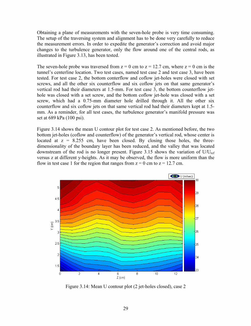
Obtaining a plane of measurements with the seven-hole probe is very time consuming. The setup of the traversing system and alignment has to be done very carefully to reduce the measurement errors. In order to expedite the generator’s correction and avoid major changes to the turbulence generator, only the flow around one of the central rods, as illustrated in Figure 3.13, has been tested. The seven-hole probe was traversed from z = 0 cm to z = 12.7 cm, where z = 0 cm is the tunnel’s centerline location. Two test cases, named test case 2 and test case 3, have been tested. For test case 2, the bottom conterflow and coflow jet-holes were closed with set screws, and all the other six counterflow and six coflow jets on that same generator’s vertical rod had their diameters at 1.5-mm. For test case 3, the bottom counterflow jet-hole was closed with a set screw, and the bottom coflow jet-hole was closed with a set screw, which had a 0.75-mm diameter hole drilled through it. All the other six counterflow and six coflow jets on that same vertical rod had their diameters kept at 1.5-mm. As a reminder, for all test cases, the turbulence generator’s manifold pressure was set at 689 kPa (100 psi). Figure 3.14 shows the mean U contour plot for test case 2. As mentioned before, the two bottom jet-holes (coflow and counterflow) of the generator’s vertical rod, whose center is located at z = 8.255 cm, have been closed. By closing those holes, the three-dimensionality of the boundary layer has been reduced, and the valley that was located downstream of the rod is no longer present. Figure 3.15 shows the variation of U/Uref versus z at different y-heights. As it may be observed, the flow is more uniform than the flow in test case 1 for the region that ranges from z = 0 cm to z = 12.7 cm.

Figure 3.14: Mean U contour plot (2 jet-holes closed), case 2

29

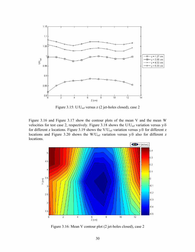
Figure 3.15: U/Uref versus z (2 jet-holes closed), case 2

Figure 3.16 and Figure 3.17 show the contour plots of the mean V and the mean W velocities for test case 2, respectively. Figure 3.18 shows the U/Uref variation versus y/δ for different z locations. Figure 3.19 shows the V/Uref variation versus y/δ for different z locations and Figure 3.20 shows the W/Uref variation versus y/δ also for different z locations.

Figure 3.16: Mean V contour plot (2 jet-holes closed), case 2

30

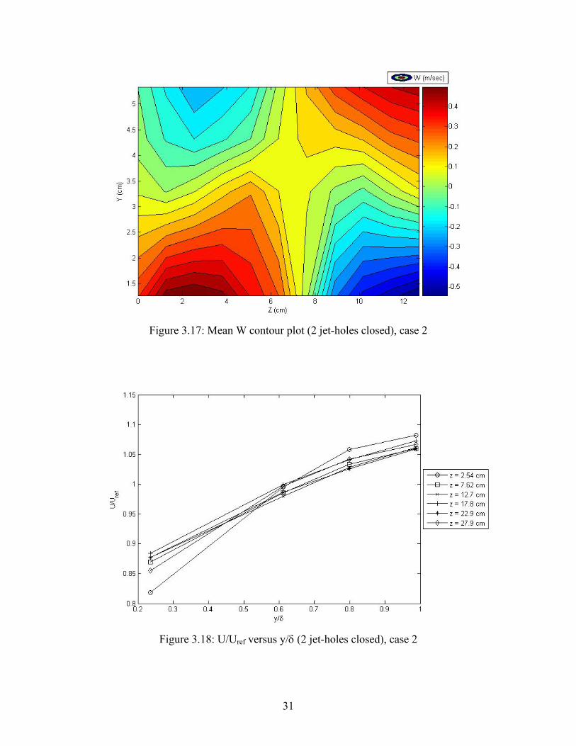
Figure 3.17: Mean W contour plot (2 jet-holes closed), case 2

Figure 3.18: U/Uref versus y/δ (2 jet-holes closed), case 2

31

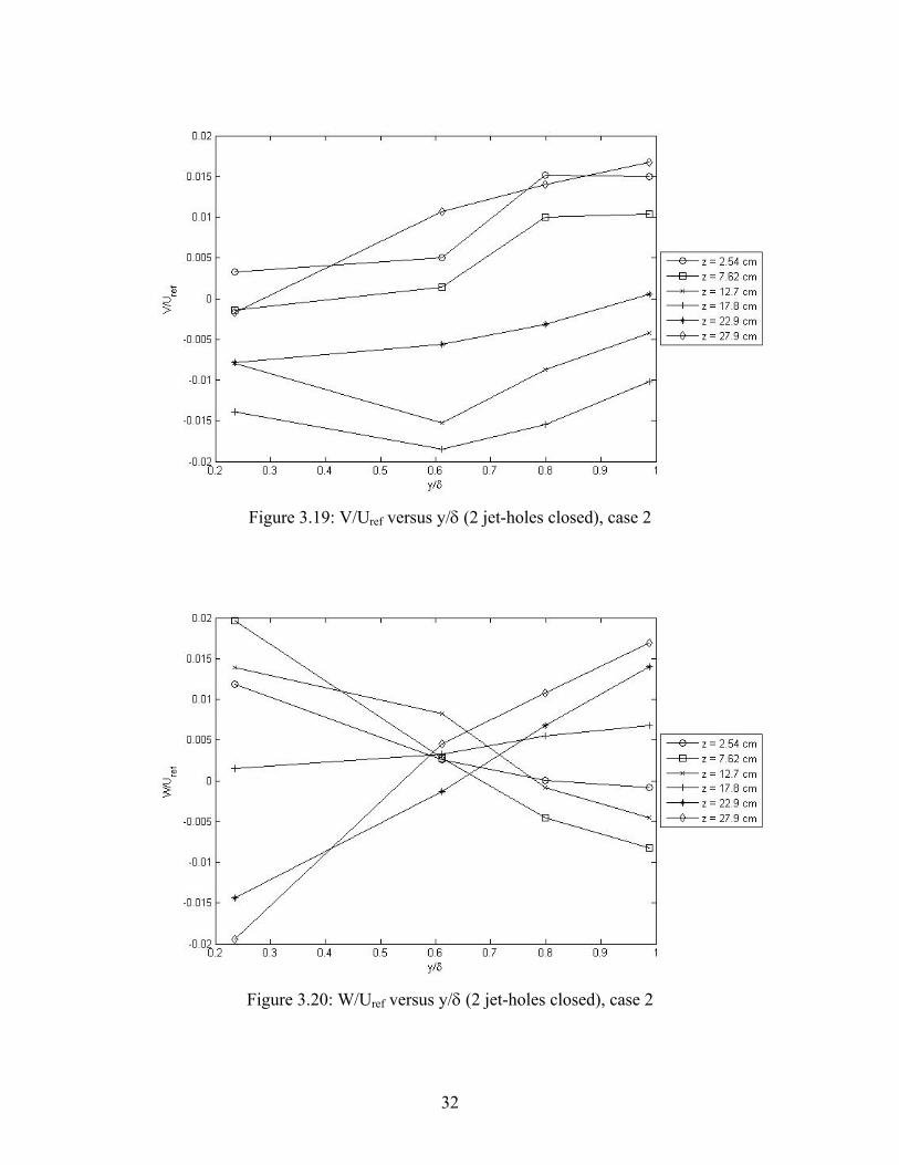
Figure 3.19: V/Uref versus y/δ (2 jet-holes closed), case 2

Figure 3.20: W/Uref versus y/δ (2 jet-holes closed), case 2

32

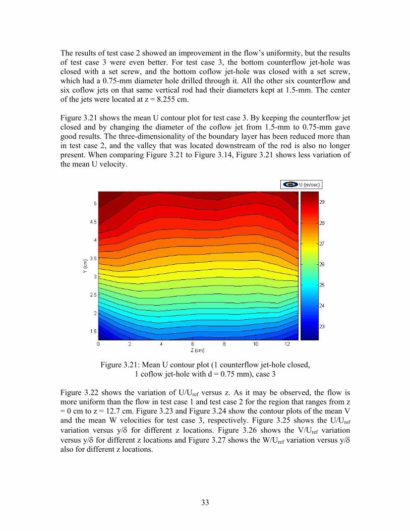
The results of test case 2 showed an improvement in the flow’s uniformity, but the results of test case 3 were even better. For test case 3, the bottom counterflow jet-hole was closed with a set screw, and the bottom coflow jet-hole was closed with a set screw, which had a 0.75-mm diameter hole drilled through it. All the other six counterflow and six coflow jets on that same vertical rod had their diameters kept at 1.5-mm. The center of the jets were located at z = 8.255 cm. Figure 3.21 shows the mean U contour plot for test case 3. By keeping the counterflow jet closed and by changing the diameter of the coflow jet from 1.5-mm to 0.75-mm gave good results. The three-dimensionality of the boundary layer has been reduced more than in test case 2, and the valley that was located downstream of the rod is also no longer present. When comparing Figure 3.21 to Figure 3.14, Figure 3.21 shows less variation of the mean U velocity.

Figure 3.21: Mean U contour plot (1 counterflow jet-hole closed,

1 coflow jet-hole with d = 0.75 mm), case 3

Figure 3.22 shows the variation of U/Uref versus z. As it may be observed, the flow is more uniform than the flow in test case 1 and test case 2 for the region that ranges from z = 0 cm to z = 12.7 cm. Figure 3.23 and Figure 3.24 show the contour plots of the mean V and the mean W velocities for test case 3, respectively. Figure 3.25 shows the U/Uref variation versus y/δ for different z locations. Figure 3.26 shows the V/Uref variation versus y/δ for different z locations and Figure 3.27 shows the W/Uref variation versus y/δ also for different z locations.

33

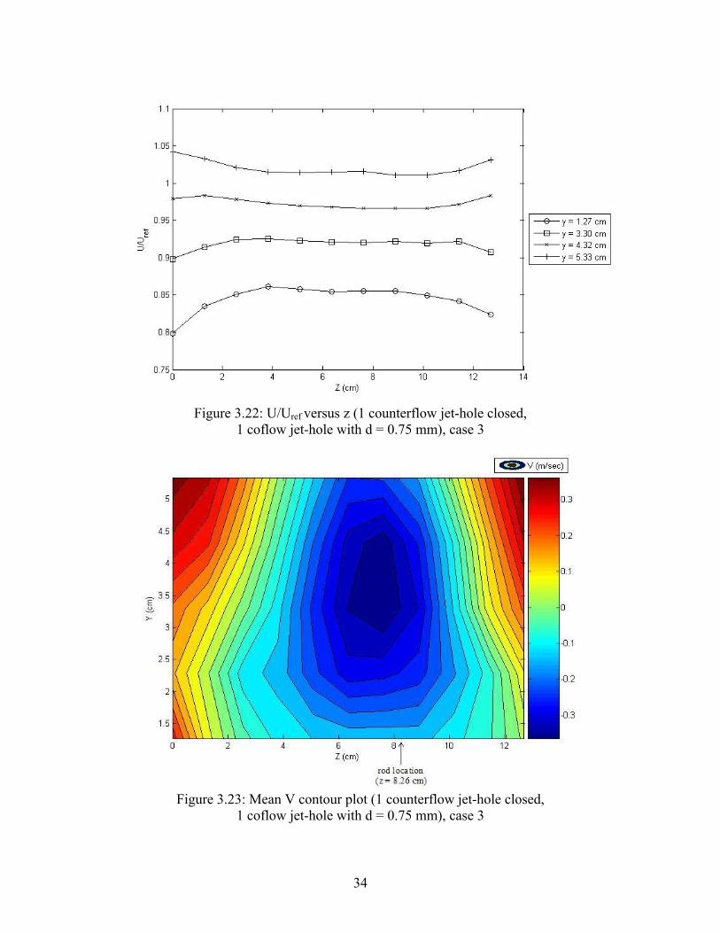
Figure 3.22: U/Uref versus z (1 counterflow jet-hole closed,

1 coflow jet-hole with d = 0.75 mm), case 3

Figure 3.23: Mean V contour plot (1 counterflow jet-hole closed,

1 coflow jet-hole with d = 0.75 mm), case 3

34

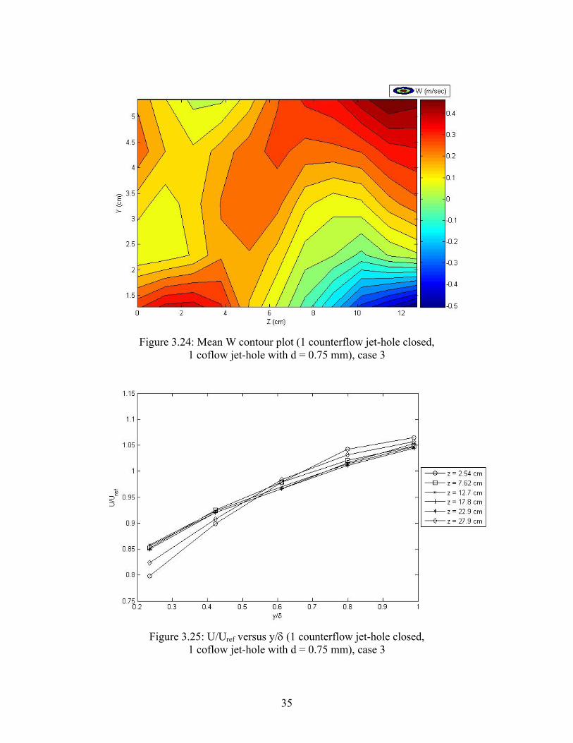
Figure 3.24: Mean W contour plot (1 counterflow jet-hole closed,

1 coflow jet-hole with d = 0.75 mm), case 3

Figure 3.25: U/Uref versus y/δ (1 counterflow jet-hole closed,

1 coflow jet-hole with d = 0.75 mm), case 3

35

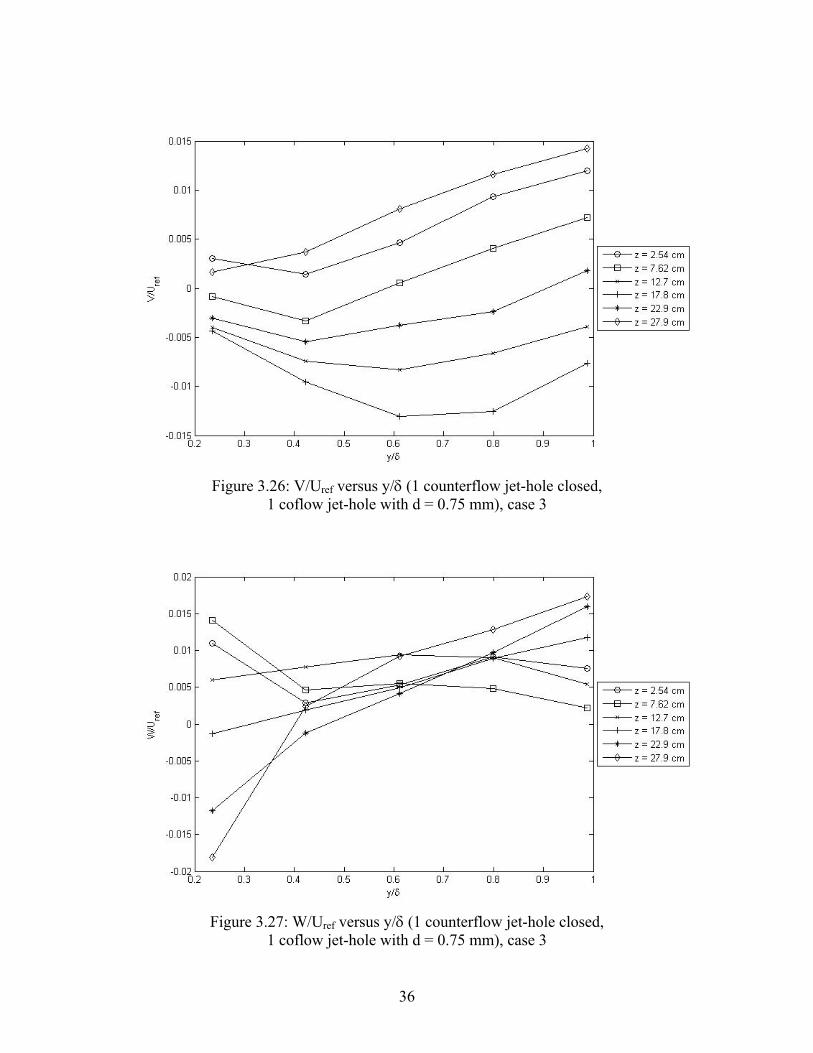
Figure 3.26: V/Uref versus y/δ (1 counterflow jet-hole closed,

1 coflow jet-hole with d = 0.75 mm), case 3

Figure 3.27: W/Uref versus y/δ (1 counterflow jet-hole closed,

1 coflow jet-hole with d = 0.75 mm), case 3

36

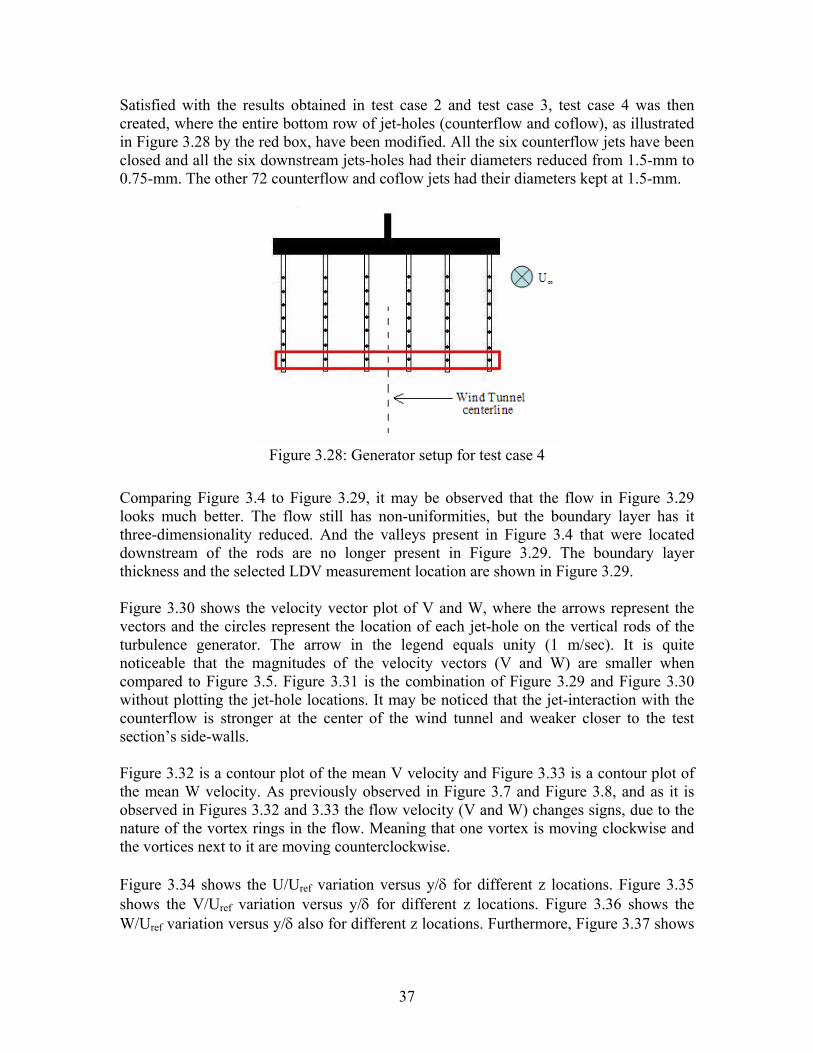
Satisfied with the results obtained in test case 2 and test case 3, test case 4 was then created, where the entire bottom row of jet-holes (counterflow and coflow), as illustrated in Figure 3.28 by the red box, have been modified. All the six counterflow jets have been closed and all the six downstream jets-holes had their diameters reduced from 1.5-mm to 0.75-mm. The other 72 counterflow and coflow jets had their diameters kept at 1.5-mm.

Figure 3.28: Generator setup for test case 4

Comparing Figure 3.4 to Figure 3.29, it may be observed that the flow in Figure 3.29 looks much better. The flow still has non-uniformities, but the boundary layer has it three-dimensionality reduced. And the valleys present in Figure 3.4 that were located downstream of the rods are no longer present in Figure 3.29. The boundary layer thickness and the selected LDV measurement location are shown in Figure 3.29. Figure 3.30 shows the velocity vector plot of V and W, where the arrows represent the vectors and the circles represent the location of each jet-hole on the vertical rods of the turbulence generator. The arrow in the legend equals unity (1 m/sec). It is quite noticeable that the magnitudes of the velocity vectors (V and W) are smaller when compared to Figure 3.5. Figure 3.31 is the combination of Figure 3.29 and Figure 3.30 without plotting the jet-hole locations. It may be noticed that the jet-interaction with the counterflow is stronger at the center of the wind tunnel and weaker closer to the test section’s side-walls. Figure 3.32 is a contour plot of the mean V velocity and Figure 3.33 is a contour plot of the mean W velocity. As previously observed in Figure 3.7 and Figure 3.8, and as it is observed in Figures 3.32 and 3.33 the flow velocity (V and W) changes signs, due to the nature of the vortex rings in the flow. Meaning that one vortex is moving clockwise and the vortices next to it are moving counterclockwise. Figure 3.34 shows the U/Uref variation versus y/δ for different z locations. Figure 3.35 shows the V/Uref variation versus y/δ for different z locations. Figure 3.36 shows the W/Uref variation versus y/δ also for different z locations. Furthermore, Figure 3.37 shows

37

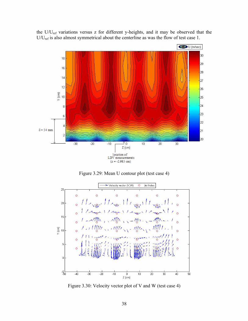
the U/Uref variations versus z for different y-heights, and it may be observed that the U/Uref is also almost symmetrical about the centerline as was the flow of test case 1.

Figure 3.29: Mean U contour plot (test case 4)

Figure 3.30: Velocity vector plot of V and W (test case 4)

38

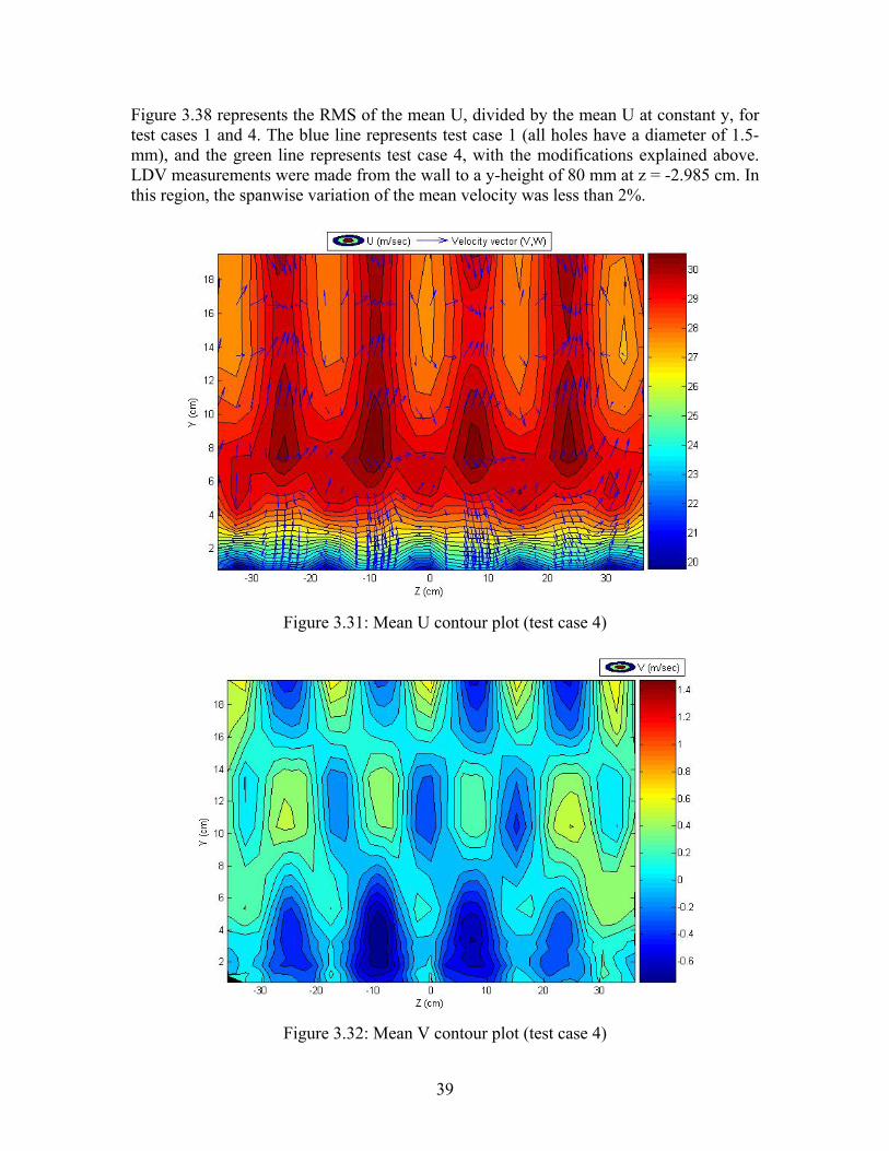
Figure 3.38 represents the RMS of the mean U, divided by the mean U at constant y, for test cases 1 and 4. The blue line represents test case 1 (all holes have a diameter of 1.5-mm), and the green line represents test case 4, with the modifications explained above. LDV measurements were made from the wall to a y-height of 80 mm at z = -2.985 cm. In this region, the spanwise variation of the mean velocity was less than 2%.

Figure 3.31: Mean U contour plot (test case 4)

Figure 3.32: Mean V contour plot (test case 4)

39

Figure 3.33: Mean W contour plot (test case 4)

Figure 3.34: U/Uref versus y/δ (test case 4)

40

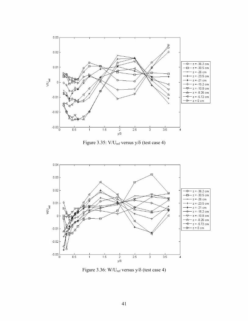
Figure 3.35: V/Uref versus y/δ (test case 4)

Figure 3.36: W/Uref versus y/δ (test case 4)

41

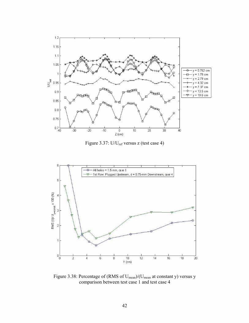
Figure 3.37: U/Uref versus z (test case 4)

Figure 3.38: Percentage of (RMS of Umean)/(Umean at constant y) versus y comparison between test case 1 and test case 4

42

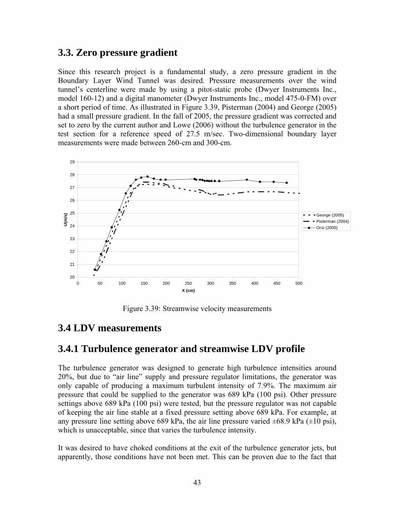
3.3. Zero pressure gradient Since this research project is a fundamental study, a zero pressure gradient in the Boundary Layer Wind Tunnel was desired. Pressure measurements over the wind tunnel’s centerline were made by using a pitot-static probe (Dwyer Instruments Inc., model 160-12) and a digital manometer (Dwyer Instruments Inc., model 475-0-FM) over a short period of time. As illustrated in Figure 3.39, Pisterman (2004) and George (2005) had a small pressure gradient. In the fall of 2005, the pressure gradient was corrected and set to zero by the current author and Lowe (2006) without the turbulence generator in the test section for a reference speed of 27.5 m/sec. Two-dimensional boundary layer measurements were made between 260-cm and 300-cm.

20

21

22

23

24

25

26

27

28

29

0 50 100 150 200 250 300 350 400 450 500

X (cm)

U(m

/s) George (2005)

Pisterman (2004)Orsi (2005)

Figure 3.39: Streamwise velocity measurements

3.4 LDV measurements

3.4.1 Turbulence generator and streamwise LDV profile The turbulence generator was designed to generate high turbulence intensities around 20%, but due to “air line” supply and pressure regulator limitations, the generator was only capable of producing a maximum turbulent intensity of 7.9%. The maximum air pressure that could be supplied to the generator was 689 kPa (100 psi). Other pressure settings above 689 kPa (100 psi) were tested, but the pressure regulator was not capable of keeping the air line stable at a fixed pressure setting above 689 kPa. For example, at any pressure line setting above 689 kPa, the air line pressure varied ±68.9 kPa (±10 psi), which is unacceptable, since that varies the turbulence intensity. It was desired to have choked conditions at the exit of the turbulence generator jets, but apparently, those conditions have not been met. This can be proven due to the fact that

43

increasing the air line pressure above 689 kPa increases the turbulence intensity. Therefore, if the turbulence intensity is changing it means that the flow is still being affected by the pressure. If the flow was choked, increasing the air line pressure would not affect the turbulence intensity. The mass flow rate and volumetric flow rate of the Boundary Layer Wind Tunnel were calculated. For a reference velocity of 27.5 m/sec, the mass flow rate and the volumetric

flow rate of the Boundary Layer Wind Tunnel were found to be and Q = 6.39 m

sec/12.7 Kgm =•

3/sec, respectively. Since the temperature at the turbulence generator jets’-exit could not be measured and since the jet-flow was not choked, the mass flow rate of the jets could not be calculated. An estimate was obtained by using the change in velocity inside the Boundary Layer Wind Tunnel when the turbulence generator was on. The LDV data have shown that the average velocity in the wind tunnel has increased by 1.1 m/sec when the turbulence generator was turned on. Based on this value the mass flow rate of the turbulence generator was estimated to be approximately equal to 0.28 Kg/sec (for modified generator – 78 jets: 6 with d = 0.75 mm and 72 with d = 1.5 mm). As mentioned in Section 3.2 of this chapter, the LDV probe was fixed at z = -2.985 cm for the normal and streamwise velocity-profile measurements; refer to Figure 3.29. For the streamwise velocity profile, the LDV probe could only be traversed from x = 71.12 cm to x = 88.9 cm, where x = 0 cm was at the exit of the generator’s coflow jet-holes. Some of the wind tunnel brackets, located under the test section, which are used to level and fix the wind tunnel in place, limit the movement of the platform on which the LDV probe sits. Figure 3.40 illustrates the turbulence intensity at different x-locations downstream of the generator. As it may be observed, the turbulence intensity does not decay. At 71.12 cm away from the generator, the turbulence intensity is approximately equal to 7.4%. At x = 83.82 cm the turbulence intensity is approximately equal to 7.9%. Finally, at the last point (x = 88.9 cm) the turbulence intensity decreases to 7.4%. Of all the previous studies reviewed in this research project, only the experiments of Hollingsworth and Bourgogne (1995) show no turbulence decay. The turbulence intensity (TI) was calculated based on the local Turbulent Kinetic Energy (TKE) and the mean velocity (U) by using the following equation:

%1002)()()( 222

×

++

=U

wvu

TI (3.1)

44

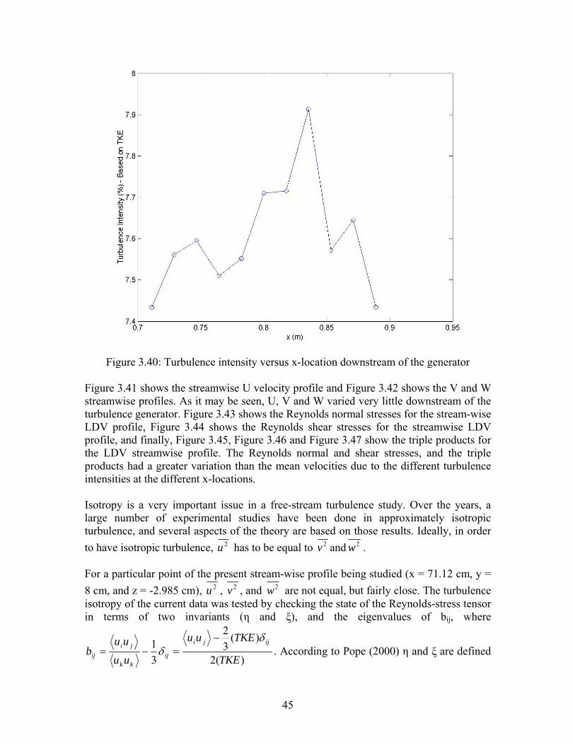
Figure 3.40: Turbulence intensity versus x-location downstream of the generator

Figure 3.41 shows the streamwise U velocity profile and Figure 3.42 shows the V and W streamwise profiles. As it may be seen, U, V and W varied very little downstream of the turbulence generator. Figure 3.43 shows the Reynolds normal stresses for the stream-wise LDV profile, Figure 3.44 shows the Reynolds shear stresses for the streamwise LDV profile, and finally, Figure 3.45, Figure 3.46 and Figure 3.47 show the triple products for the LDV streamwise profile. The Reynolds normal and shear stresses, and the triple products had a greater variation than the mean velocities due to the different turbulence intensities at the different x-locations. Isotropy is a very important issue in a free-stream turbulence study. Over the years, a large number of experimental studies have been done in approximately isotropic turbulence, and several aspects of the theory are based on those results. Ideally, in order to have isotropic turbulence, 2u has to be equal to 2v and 2w . For a particular point of the present stream-wise profile being studied (x = 71.12 cm, y = 8 cm, and z = -2.985 cm), 2u , 2v , and 2w are not equal, but fairly close. The turbulence isotropy of the current data was tested by checking the state of the Reynolds-stress tensor in terms of two invariants (η and ξ), and the eigenvalues of bij, where

)(2

)(32

31

TKE

TKEuu

uu

uub

ijji

ijkk

jiij

δδ

−=−= . According to Pope (2000) η and ξ are defined

45

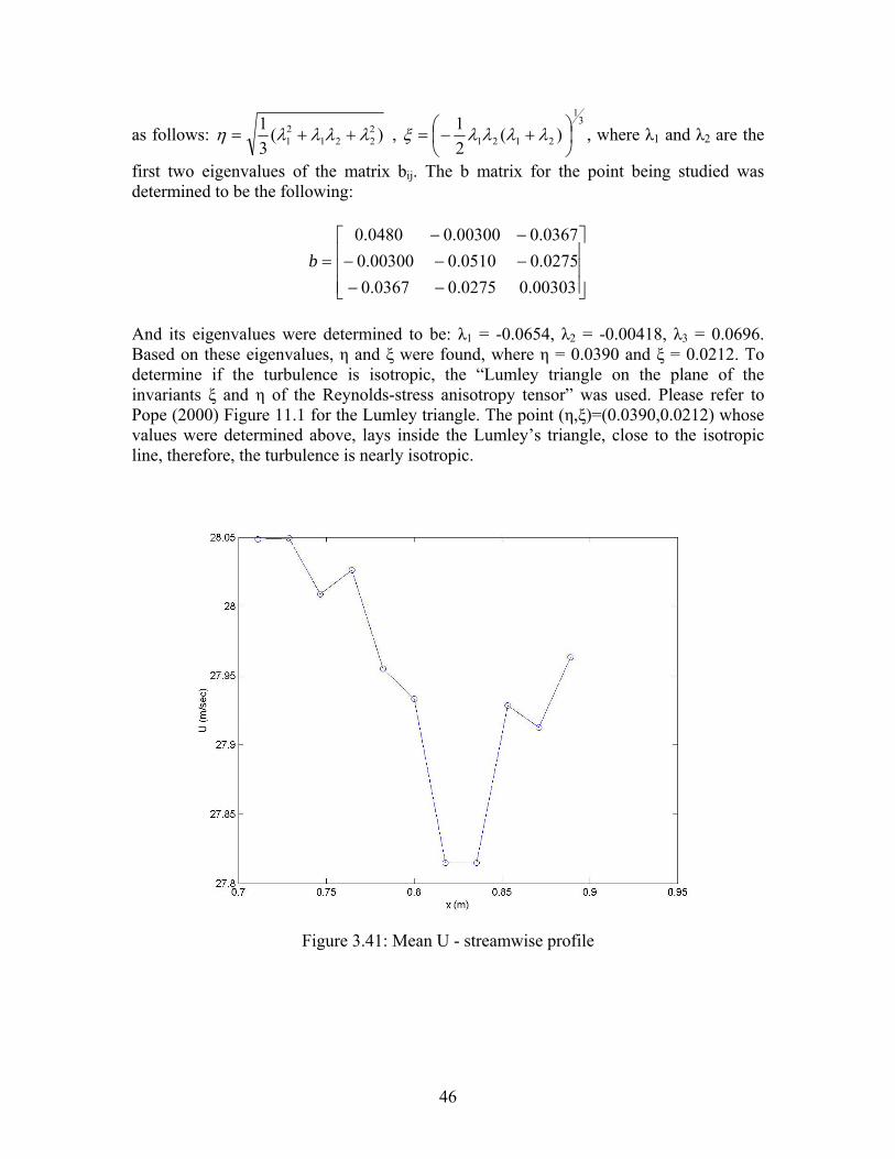
as follows: 3

1

21212221

21 )(

21 , )(

31

⎟⎠⎞

⎜⎝⎛ +−=++= λλλλξλλλλη , where λ1 and λ2 are the

first two eigenvalues of the matrix bij. The b matrix for the point being studied was determined to be the following:

⎥⎥⎥

⎦

⎤

⎢⎢⎢

⎣

⎡

−−−−−−−

=00303.00275.00367.0

0275.00510.000300.00367.000300.00480.0

b

And its eigenvalues were determined to be: λ1 = -0.0654, λ2 = -0.00418, λ3 = 0.0696. Based on these eigenvalues, η and ξ were found, where η = 0.0390 and ξ = 0.0212. To determine if the turbulence is isotropic, the “Lumley triangle on the plane of the invariants ξ and η of the Reynolds-stress anisotropy tensor” was used. Please refer to Pope (2000) Figure 11.1 for the Lumley triangle. The point (η,ξ)=(0.0390,0.0212) whose values were determined above, lays inside the Lumley’s triangle, close to the isotropic line, therefore, the turbulence is nearly isotropic.

Figure 3.41: Mean U - streamwise profile

46

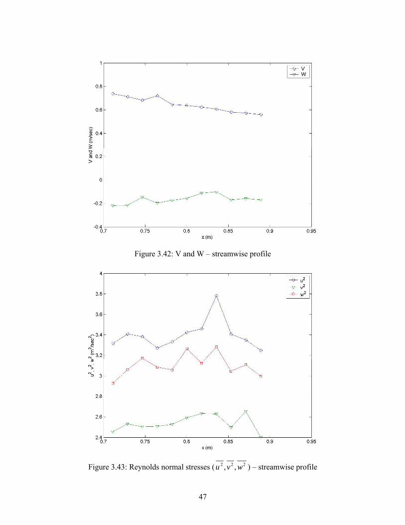
Figure 3.42: V and W – streamwise profile

Figure 3.43: Reynolds normal stresses ( 222 ,, wvu ) – streamwise profile

47

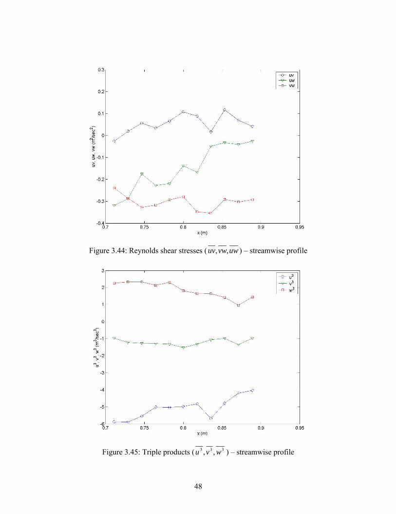
Figure 3.44: Reynolds shear stresses ( uwvwuv ,, ) – streamwise profile

Figure 3.45: Triple products ( 333 ,, wvu ) – streamwise profile

48

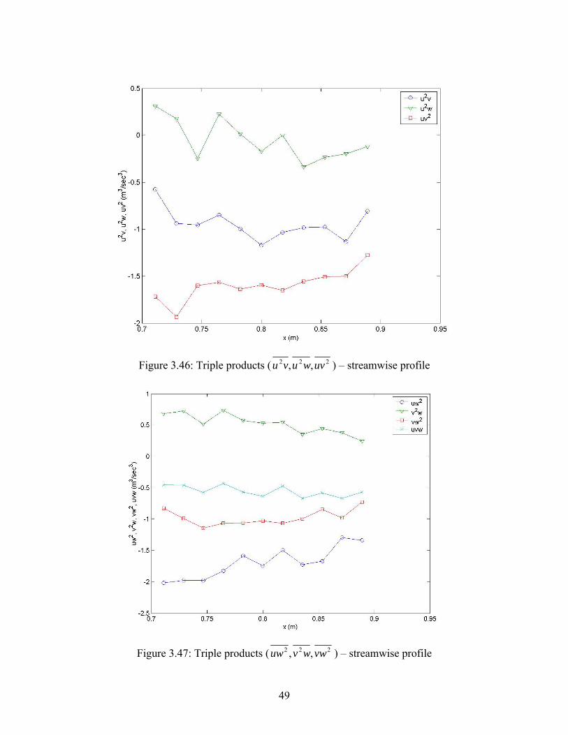
Figure 3.46: Triple products ( 222 ,, uvwuvu ) – streamwise profile

Figure 3.47: Triple products ( 222 ,, vwwvuw ) – streamwise profile

49

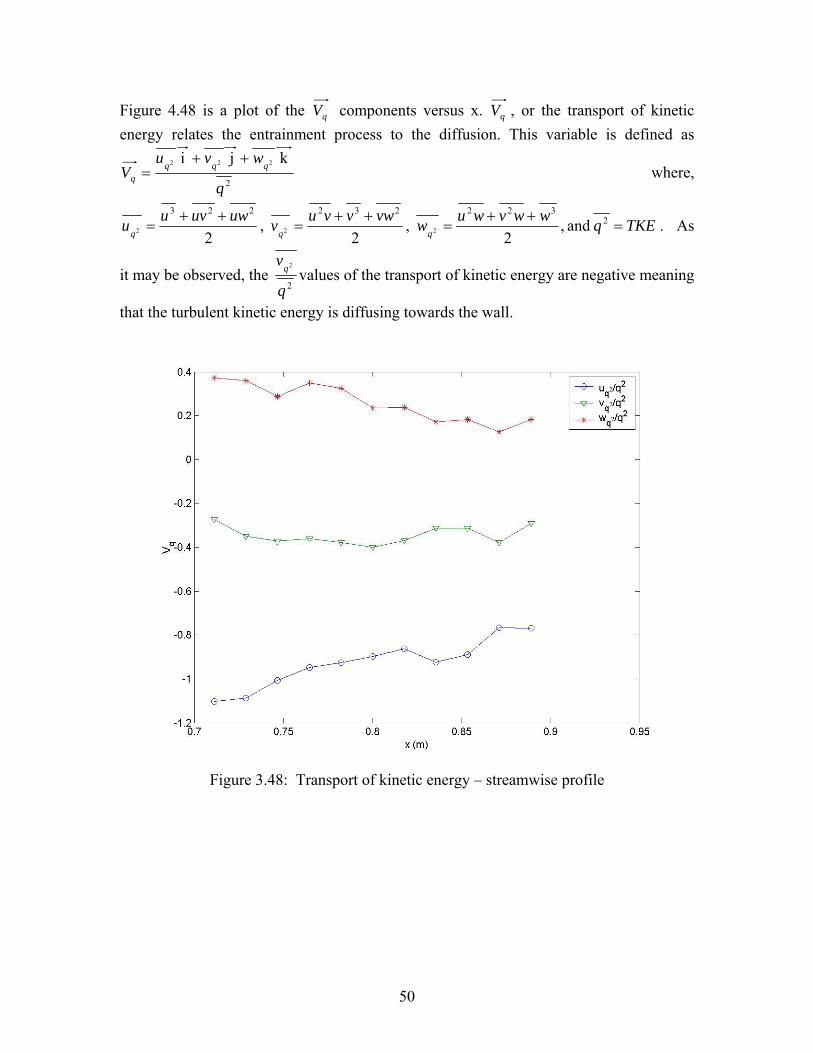
Figure 4.48 is a plot of the qV components versus x. qV , or the transport of kinetic energy relates the entrainment process to the diffusion. This variable is defined as

2

k j i 222

q

wvuV qqq

q

++= where,

TKEqwwvwuwvwvvuvuwuvuuqqq

=++

=++

=++

= 2322232223

and ,2

, 2

, 2 222 . As

it may be observed, the 2

2

q

vq values of the transport of kinetic energy are negative meaning

that the turbulent kinetic energy is diffusing towards the wall.

Figure 3.48: Transport of kinetic energy – streamwise profile

50

3.4.2 LDV velocity corrections Based on the paper by Durst et al. (1992), the quantities U, 2u and 3u were corrected. The following equations were used for the corrections:

⎟⎟⎠

⎞⎜⎜⎝

⎛+= 2

22 )(24

)(dy

yUddyUU , equation # 10 of Durst (1992)

22

22 )(12

)( ⎟⎟⎠

⎞⎜⎜⎝

⎛+=

dyyUddyuu , equation # 12 of Durst (1992)

⎟⎟⎠

⎞⎜⎜⎝

⎛+⎟⎟

⎠

⎞⎜⎜⎝

⎛⎟⎟⎠

⎞⎜⎜⎝

⎛+= 2

322

2

2233 )(

24)()(

4)(

dyyudd

dyyUd

dyyuddyuu , equation # 13 of Durst (1992)

Where, 32 and , uuU are the measured values and )( and )(),( 32 yuyuyU are the true

values. The value for d (the measurement volume size) was determined from the 2u data (Figure 3.56) and was equal to 130 µm. After the calculations were made, the corrected U values did look as good as the uncorrected values when compared to the law of the wall in the sublayer. The corrected results for 3u were extremely different than the values for the uncorrected 3u . The corrected values of 2u seemed better than the uncorrected values. The LDV measurements already have very small uncertainty, see section 3.6. The U and 3u corrections use second derivatives which seem to have larger uncertainties than the actual measurements. The 2u correction only uses a first derivative, which seems to have a small uncertainty since the corrected values of 2u looked better than the uncorrected results. Figure 3.18 shows the comparison of the corrected and uncorrected values of the mean U profile for the case without high free-stream turbulence effects. Figure 3.19 shows the comparison of the corrected and uncorrected values of the mean U profile for the case with high free-stream turbulence effects. As discussed by Kuhl (2000) for LDV measurements where 3-components (x, y, z) are measured, the velocity bias for these measurements is equal to zero.

51

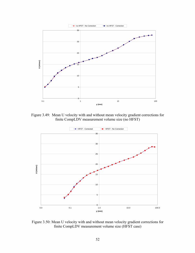
0

5

10

15

20

25

30

0.1 1 10 100

y (mm)

U (m

/sec

)

no HFST - No Correction no HFST - Correction

Figure 3.49: Mean U velocity with and without mean velocity gradient corrections for finite CompLDV measurement volume size (no HFST)

0

5

10

15

20

25

30

35

0.0 0.1 1.0 10.0 100.0

y (mm)

U (m

/sec

)

HFST - Corrected HFST - No Correction

Figure 3.50: Mean U velocity with and without mean velocity gradient corrections for finite CompLDV measurement volume size (HFST case)

52

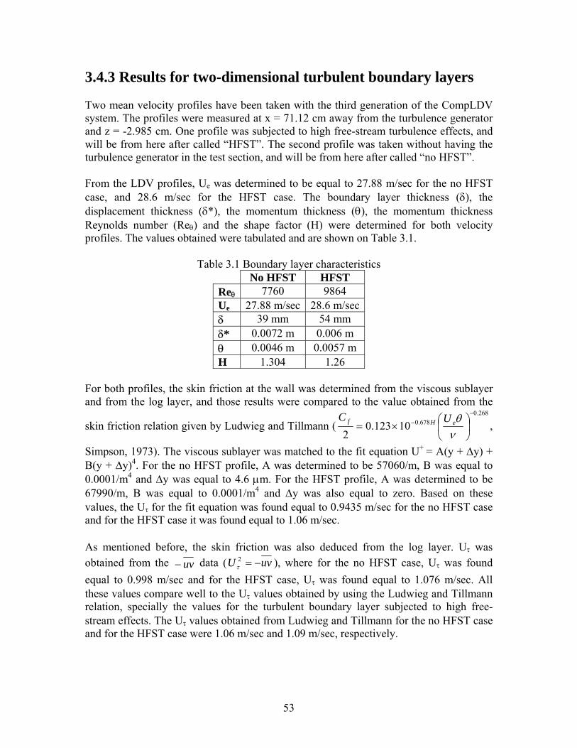
3.4.3 Results for two-dimensional turbulent boundary layers Two mean velocity profiles have been taken with the third generation of the CompLDV system. The profiles were measured at x = 71.12 cm away from the turbulence generator and z = -2.985 cm. One profile was subjected to high free-stream turbulence effects, and will be from here after called “HFST”. The second profile was taken without having the turbulence generator in the test section, and will be from here after called “no HFST”. From the LDV profiles, Ue was determined to be equal to 27.88 m/sec for the no HFST case, and 28.6 m/sec for the HFST case. The boundary layer thickness (δ), the displacement thickness (δ*), the momentum thickness (θ), the momentum thickness Reynolds number (Reθ) and the shape factor (H) were determined for both velocity profiles. The values obtained were tabulated and are shown on Table 3.1.

Table 3.1 Boundary layer characteristics No HFST HFST

Reθ 7760 9864 Ue 27.88 m/sec 28.6 m/secδ 39 mm 54 mm δ* 0.0072 m 0.006 m θ 0.0046 m 0.0057 m H 1.304 1.26

For both profiles, the skin friction at the wall was determined from the viscous sublayer and from the log layer, and those results were compared to the value obtained from the

skin friction relation given by Ludwieg and Tillmann (268.0

678.010123.02

−− ⎟

⎠⎞

⎜⎝⎛×=

νθeHf UC

,

Simpson, 1973). The viscous sublayer was matched to the fit equation U+ = A(y + ∆y) + B(y + ∆y)4. For the no HFST profile, A was determined to be 57060/m, B was equal to 0.0001/m4 and ∆y was equal to 4.6 µm. For the HFST profile, A was determined to be 67990/m, B was equal to 0.0001/m4 and ∆y was also equal to zero. Based on these values, the Uτ for the fit equation was found equal to 0.9435 m/sec for the no HFST case and for the HFST case it was found equal to 1.06 m/sec. As mentioned before, the skin friction was also deduced from the log layer. Uτ was obtained from the uv− data ( uvU −=2

τ ), where for the no HFST case, Uτ was found equal to 0.998 m/sec and for the HFST case, Uτ was found equal to 1.076 m/sec. All these values compare well to the Uτ values obtained by using the Ludwieg and Tillmann relation, specially the values for the turbulent boundary layer subjected to high free-stream effects. The Uτ values obtained from Ludwieg and Tillmann for the no HFST case and for the HFST case were 1.06 m/sec and 1.09 m/sec, respectively.

53

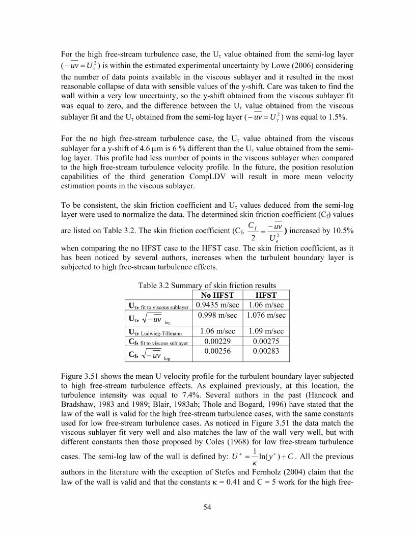
For the high free-stream turbulence case, the Uτ value obtained from the semi-log layer ( 2

τUuv =− ) is within the estimated experimental uncertainty by Lowe (2006) considering the number of data points available in the viscous sublayer and it resulted in the most reasonable collapse of data with sensible values of the y-shift. Care was taken to find the wall within a very low uncertainty, so the y-shift obtained from the viscous sublayer fit was equal to zero, and the difference between the Uτ value obtained from the viscous sublayer fit and the Uτ obtained from the semi-log layer ( 2

τUuv =− ) was equal to 1.5%. For the no high free-stream turbulence case, the Uτ value obtained from the viscous sublayer for a y-shift of 4.6 µm is 6 % different than the Uτ value obtained from the semi-log layer. This profile had less number of points in the viscous sublayer when compared to the high free-stream turbulence velocity profile. In the future, the position resolution capabilities of the third generation CompLDV will result in more mean velocity estimation points in the viscous sublayer. To be consistent, the skin friction coefficient and Uτ values deduced from the semi-log layer were used to normalize the data. The determined skin friction coefficient (Cf) values

are listed on Table 3.2. The skin friction coefficient (Cf, 22 e

f

UuvC −

= ) increased by 10.5%

when comparing the no HFST case to the HFST case. The skin friction coefficient, as it has been noticed by several authors, increases when the turbulent boundary layer is subjected to high free-stream turbulence effects.

Table 3.2 Summary of skin friction results No HFST HFST Uτ, fit to viscous sublayer 0.9435 m/sec 1.06 m/sec

Uτ, log uv− 0.998 m/sec 1.076 m/sec

Uτ, Ludwieg-Tillmann 1.06 m/sec 1.09 m/sec Cf, fit to viscous sublayer 0.00229 0.00275 Cf, log uv− 0.00256 0.00283

Figure 3.51 shows the mean U velocity profile for the turbulent boundary layer subjected to high free-stream turbulence effects. As explained previously, at this location, the turbulence intensity was equal to 7.4%. Several authors in the past (Hancock and Bradshaw, 1983 and 1989; Blair, 1983ab; Thole and Bogard, 1996) have stated that the law of the wall is valid for the high free-stream turbulence cases, with the same constants used for low free-stream turbulence cases. As noticed in Figure 3.51 the data match the viscous sublayer fit very well and also matches the law of the wall very well, but with different constants then those proposed by Coles (1968) for low free-stream turbulence

cases. The semi-log law of the wall is defined by: CyU += ++ )ln(1κ

. All the previous

authors in the literature with the exception of Stefes and Fernholz (2004) claim that the law of the wall is valid and that the constants κ = 0.41 and C = 5 work for the high free-

54

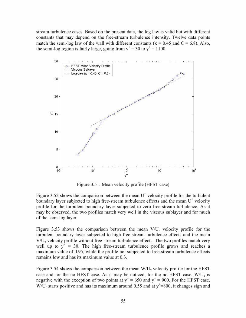
stream turbulence cases. Based on the present data, the log law is valid but with different constants that may depend on the free-stream turbulence intensity. Twelve data points match the semi-log law of the wall with different constants (κ = 0.45 and C = 6.8). Also, the semi-log region is fairly large, going from y+ = 30 to y+ = 1100.

Figure 3.51: Mean velocity profile (HFST case)

Figure 3.52 shows the comparison between the mean U+ velocity profile for the turbulent boundary layer subjected to high free-stream turbulence effects and the mean U+ velocity profile for the turbulent boundary layer subjected to zero free-stream turbulence. As it may be observed, the two profiles match very well in the viscous sublayer and for much of the semi-log layer. Figure 3.53 shows the comparison between the mean V/Uτ velocity profile for the turbulent boundary layer subjected to high free-stream turbulence effects and the mean V/Uτ velocity profile without free-stream turbulence effects. The two profiles match very well up to y+ = 30. The high free-stream turbulence profile grows and reaches a maximum value of 0.95, while the profile not subjected to free-stream turbulence effects remains low and has its maximum value at 0.3. Figure 3.54 shows the comparison between the mean W/Uτ velocity profile for the HFST case and for the no HFST case. As it may be noticed, for the no HFST case, W/Uτ is negative with the exception of two points at y+ = 650 and y+ = 900. For the HFST case, W/Uτ starts positive and has its maximum around 0.55 and at y+=800, it changes sign and

55

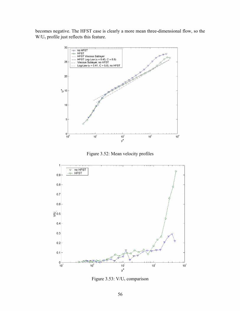
becomes negative. The HFST case is clearly a more mean three-dimensional flow, so the W/Uτ profile just reflects this feature.

Figure 3.52: Mean velocity profiles

Figure 3.53: V/Uτ comparison

56

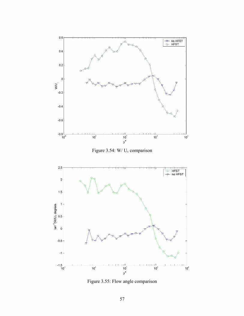
Figure 3.54: W/ Uτ comparison

Figure 3.55: Flow angle comparison

57

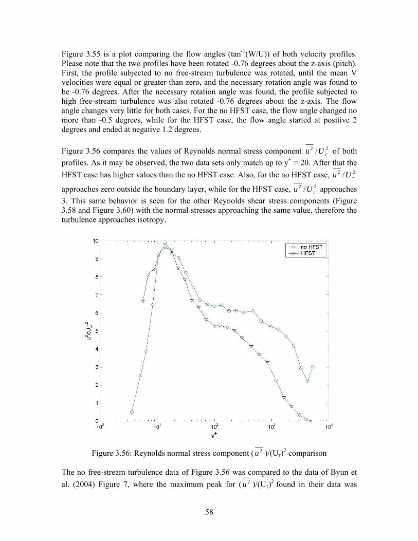
Figure 3.55 is a plot comparing the flow angles (tan-1(W/U)) of both velocity profiles. Please note that the two profiles have been rotated -0.76 degrees about the z-axis (pitch). First, the profile subjected to no free-stream turbulence was rotated, until the mean V velocities were equal or greater than zero, and the necessary rotation angle was found to be -0.76 degrees. After the necessary rotation angle was found, the profile subjected to high free-stream turbulence was also rotated -0.76 degrees about the z-axis. The flow angle changes very little for both cases. For the no HFST case, the flow angle changed no more than -0.5 degrees, while for the HFST case, the flow angle started at positive 2 degrees and ended at negative 1.2 degrees. Figure 3.56 compares the values of Reynolds normal stress component 22 / τUu of both profiles. As it may be observed, the two data sets only match up to y+ = 20. After that the HFST case has higher values than the no HFST case. Also, for the no HFST case, 22 / τUu

approaches zero outside the boundary layer, while for the HFST case, 22 / τUu approaches 3. This same behavior is seen for the other Reynolds shear stress components (Figure 3.58 and Figure 3.60) with the normal stresses approaching the same value, therefore the turbulence approaches isotropy.

Figure 3.56: Reynolds normal stress component ( 2u )/(Uτ)2 comparison

The no free-stream turbulence data of Figure 3.56 was compared to the data of Byun et al. (2004) Figure 7, where the maximum peak for ( 2u )/(Uτ)2 found in their data was

58

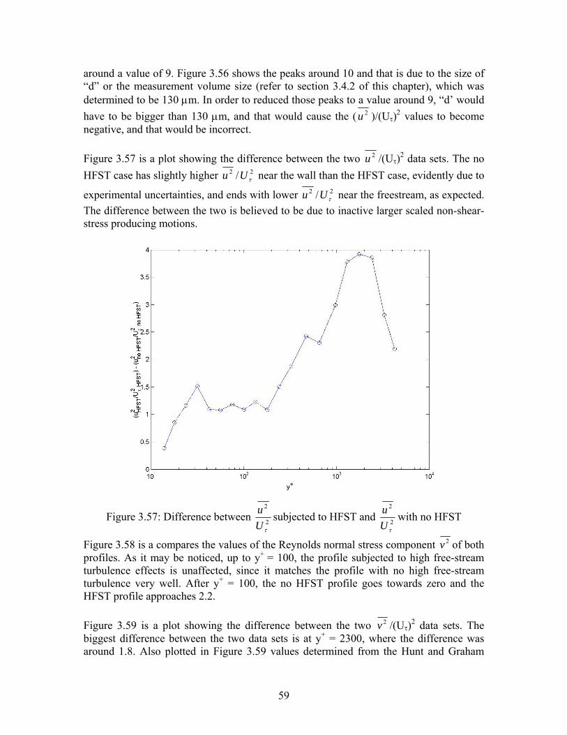
around a value of 9. Figure 3.56 shows the peaks around 10 and that is due to the size of “d” or the measurement volume size (refer to section 3.4.2 of this chapter), which was determined to be 130 µm. In order to reduced those peaks to a value around 9, “d’ would have to be bigger than 130 µm, and that would cause the ( 2u )/(Uτ)2 values to become negative, and that would be incorrect. Figure 3.57 is a plot showing the difference between the two 2u /(Uτ)2 data sets. The no HFST case has slightly higher 22 / τUu near the wall than the HFST case, evidently due to

experimental uncertainties, and ends with lower 22 / τUu near the freestream, as expected. The difference between the two is believed to be due to inactive larger scaled non-shear-stress producing motions.

Figure 3.57: Difference between 2

2

τUu subjected to HFST and 2

2

τUu with no HFST

Figure 3.58 is a compares the values of the Reynolds normal stress component 2v of both profiles. As it may be noticed, up to y+ = 100, the profile subjected to high free-stream turbulence effects is unaffected, since it matches the profile with no high free-stream turbulence very well. After y+ = 100, the no HFST profile goes towards zero and the HFST profile approaches 2.2. Figure 3.59 is a plot showing the difference between the two 2v /(Uτ)2 data sets. The biggest difference between the two data sets is at y+ = 2300, where the difference was around 1.8. Also plotted in Figure 3.59 values determined from the Hunt and Graham

59

(1978) Reynolds normal stress component 2v difference model. Hunt and Graham’s experiments had grid turbulence convected by the free-stream past a rigid surface that was moving at the same velocity as the free-stream with no inviscid rotational flow field being created.

Figure 3.58: Reynolds normal stress component ( 2v )/(Uτ)2 comparison

The Hunt and Graham (1978) model poorly predicted 22 w and u profiles but showed reasonable trends for a turbulent free-stream and moving boundary. The 2v profile for the

von Kármán spectrum is given as: 323

2

2

2

ryy

vv

=⎟⎟⎠

⎞⎜⎜⎝

⎛= +

∞

+

∞

and is given in Table 3.3.

The model does not agree well for the present data. Only two out of the four points tested matched the actual data. Therefore, the Hunt and Graham model is not valid for all Reynolds numbers and turbulence intensities.

60

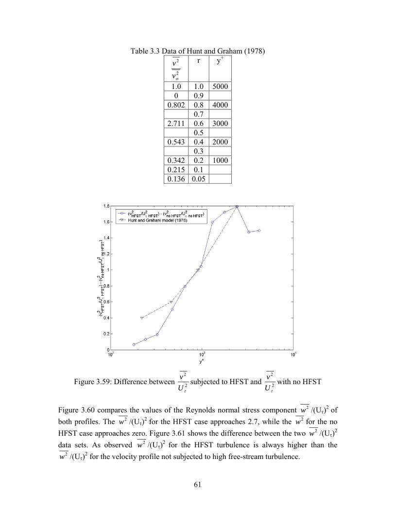
Table 3.3 Data of Hunt and Graham (1978)

2

2

∞vv

r y+

1.0 1.0 50000 0.9

0.802 0.8 4000 0.7

2.711 0.6 3000 0.5

0.543 0.4 2000 0.3

0.342 0.2 10000.215 0.1 0.136 0.05

Figure 3.59: Difference between 2

2

τUv subjected to HFST and 2

2

τUv with no HFST

Figure 3.60 compares the values of the Reynolds normal stress component 2w /(Uτ)2 of both profiles. The 2w /(Uτ)2 for the HFST case approaches 2.7, while the 2w for the no HFST case approaches zero. Figure 3.61 shows the difference between the two 2w /(Uτ)2 data sets. As observed 2w /(Uτ)2 for the HFST turbulence is always higher than the

2w /(Uτ)2 for the velocity profile not subjected to high free-stream turbulence.

61

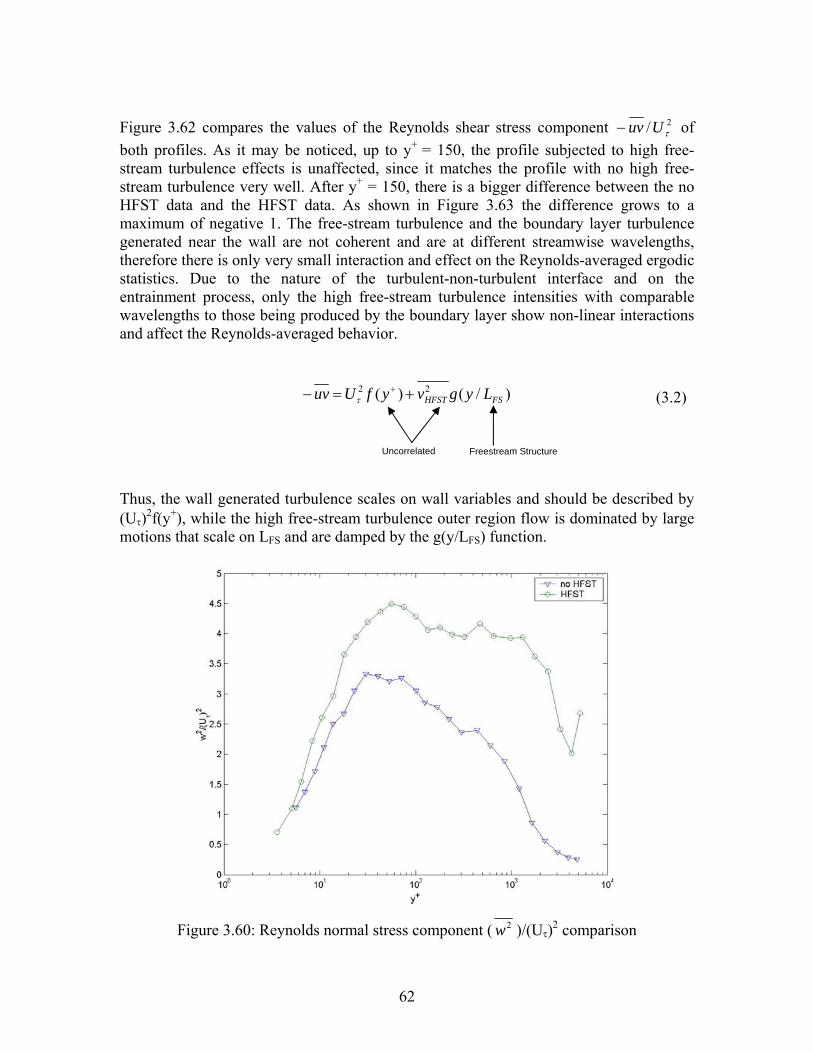
Figure 3.62 compares the values of the Reynolds shear stress component 2/ τUuv− of both profiles. As it may be noticed, up to y+ = 150, the profile subjected to high free-stream turbulence effects is unaffected, since it matches the profile with no high free-stream turbulence very well. After y+ = 150, there is a bigger difference between the no HFST data and the HFST data. As shown in Figure 3.63 the difference grows to a maximum of negative 1. The free-stream turbulence and the boundary layer turbulence generated near the wall are not coherent and are at different streamwise wavelengths, therefore there is only very small interaction and effect on the Reynolds-averaged ergodic statistics. Due to the nature of the turbulent-non-turbulent interface and on the entrainment process, only the high free-stream turbulence intensities with comparable wavelengths to those being produced by the boundary layer show non-linear interactions and affect the Reynolds-averaged behavior.

)/()( 22

FSHFST LygvyfUuv +=− +τ (3.2)

Uncorrelated Freestream Structure Thus, the wall generated turbulence scales on wall variables and should be described by (Uτ)2f(y+), while the high free-stream turbulence outer region flow is dominated by large motions that scale on LFS and are damped by the g(y/LFS) function.

Figure 3.60: Reynolds normal stress component ( 2w )/(Uτ)2 comparison

62

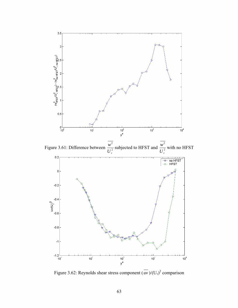
Figure 3.61: Difference between 2

2

τUw subjected to HFST and 2

2

τUw with no HFST

Figure 3.62: Reynolds shear stress component (uv )/(Uτ)2 comparison

63

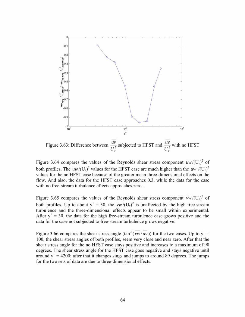
Figure 3.63: Difference between 2τU

uv subjected to HFST and 2τU

uv with no HFST

Figure 3.64 compares the values of the Reynolds shear stress component uw /(Uτ)2 of both profiles. The uw /(Uτ)2 values for the HFST case are much higher than the uw /(Uτ)2

values for the no HFST case because of the greater mean three-dimensional effects on the flow. And also, the data for the HFST case approaches 0.3, while the data for the case with no free-stream turbulence effects approaches zero. Figure 3.65 compares the values of the Reynolds shear stress component vw /(Uτ)2 of both profiles. Up to about y+ = 30, the vw /(Uτ)2 is unaffected by the high free-stream turbulence and the three-dimensional effects appear to be small within experimental. After y+ = 30, the data for the high free-stream turbulence case grows positive and the data for the case not subjected to free-stream turbulence grows negative. Figure 3.66 compares the shear stress angle (tan-1( uvvw / )) for the two cases. Up to y+ = 100, the shear stress angles of both profiles, seem very close and near zero. After that the shear stress angle for the no HFST case stays positive and increases to a maximum of 90 degrees. The shear stress angle for the HFST case goes negative and stays negative until around y+ = 4200; after that it changes sings and jumps to around 89 degrees. The jumps for the two sets of data are due to three-dimensional effects.

64

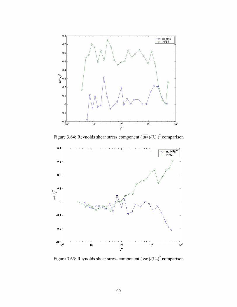
Figure 3.64: Reynolds shear stress component (uw )/(Uτ)2 comparison

Figure 3.65: Reynolds shear stress component ( vw )/(Uτ)2 comparison

65

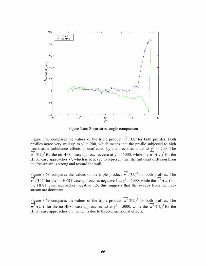
Figure 3.66: Shear stress angle comparison

Figure 3.67 compares the values of the triple product 3u /(Uτ)3for both profiles. Both profiles agree very well up to y+ = 200, which means that the profile subjected to high free-stream turbulence effects is unaffected by the free-stream up to y+ = 200. The

3u /(Uτ)3 for the no HFST case approaches zero at y+ = 5000, while the 3u /(Uτ)3 for the HFST case approaches -7, which is believed to represent that the turbulent diffusion from the freestream is strong and toward the wall. Figure 3.68 compares the values of the triple product 3v /(Uτ)3 for both profiles. The

3v /(Uτ)3 for the no HFST case approaches negative 1 at y+ = 5000, while the 3v /(Uτ)3for the HFST case approaches negative 1.5, this suggests that the sweeps from the free-stream are dominant. Figure 3.69 compares the values of the triple product 3w /(Uτ)3 for both profiles. The

3w /(Uτ)3 for the no HFST case approaches 1.5 at y+ = 5000, while the 3w /(Uτ)3 for the HFST case approaches 3.5, which is due to three-dimensional effects.

66

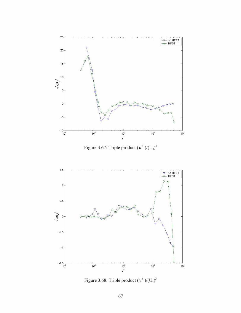
Figure 3.67: Triple product ( 3u )/(Uτ)3

Figure 3.68: Triple product ( 3v )/(Uτ)3

67

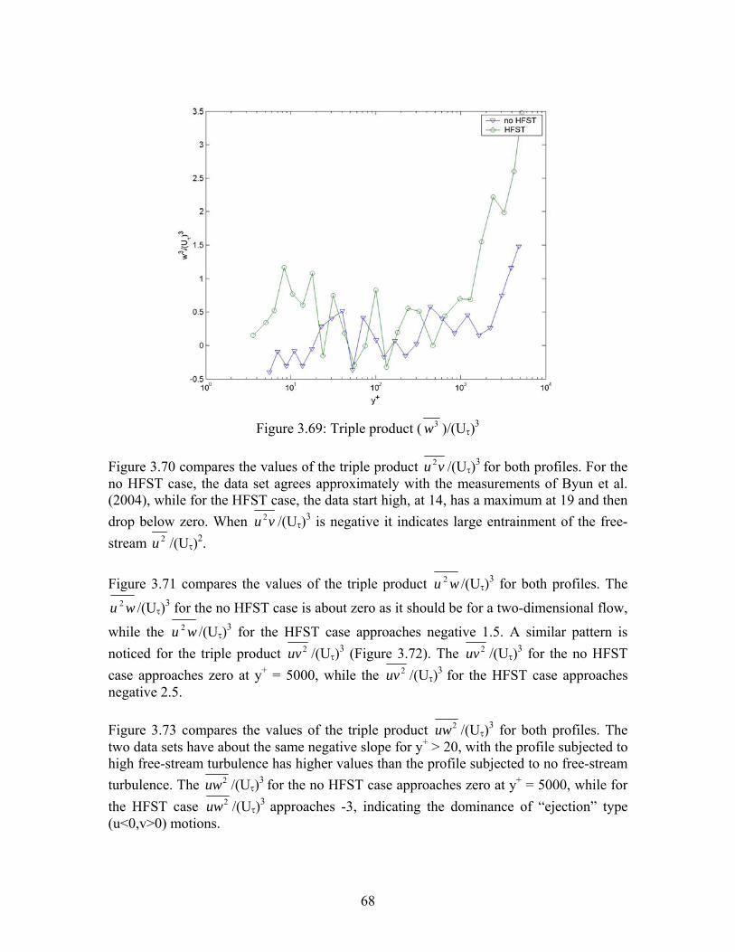
Figure 3.69: Triple product ( 3w )/(Uτ)3

Figure 3.70 compares the values of the triple product vu 2 /(Uτ)3 for both profiles. For the no HFST case, the data set agrees approximately with the measurements of Byun et al. (2004), while for the HFST case, the data start high, at 14, has a maximum at 19 and then drop below zero. When vu 2 /(Uτ)3 is negative it indicates large entrainment of the free-stream 2u /(Uτ)2.

Figure 3.71 compares the values of the triple product wu 2 /(Uτ)3 for both profiles. The

wu 2 /(Uτ)3 for the no HFST case is about zero as it should be for a two-dimensional flow,

while the wu 2 /(Uτ)3 for the HFST case approaches negative 1.5. A similar pattern is noticed for the triple product 2uv /(Uτ)3 (Figure 3.72). The 2uv /(Uτ)3 for the no HFST case approaches zero at y+ = 5000, while the 2uv /(Uτ)3 for the HFST case approaches negative 2.5. Figure 3.73 compares the values of the triple product 2uw /(Uτ)3 for both profiles. The two data sets have about the same negative slope for y+ > 20, with the profile subjected to high free-stream turbulence has higher values than the profile subjected to no free-stream turbulence. The 2uw /(Uτ)3 for the no HFST case approaches zero at y+ = 5000, while for the HFST case 2uw /(Uτ)3 approaches -3, indicating the dominance of “ejection” type (u<0,v>0) motions.

68

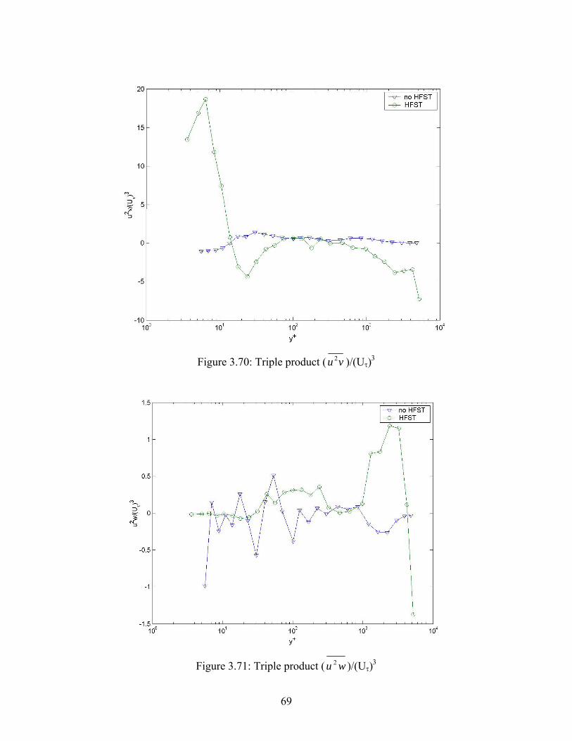
Figure 3.70: Triple product ( vu 2 )/(Uτ)3

Figure 3.71: Triple product ( wu 2 )/(Uτ)3

69

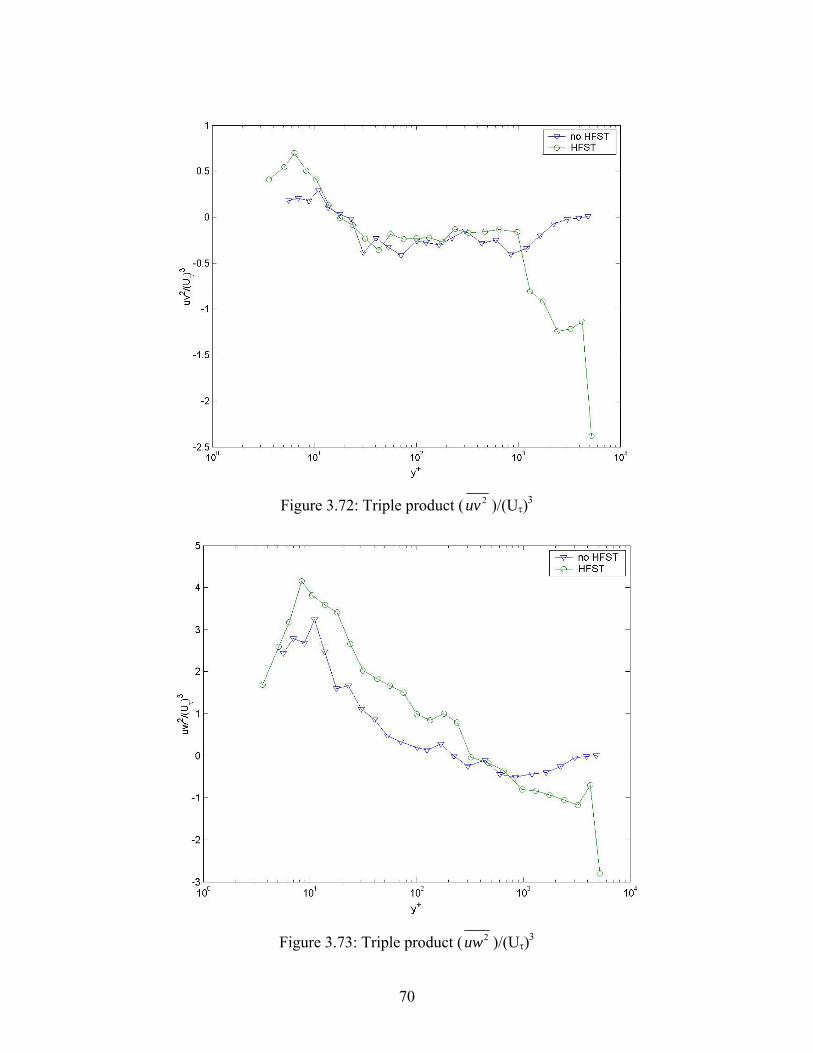
Figure 3.72: Triple product ( 2uv )/(Uτ)3

Figure 3.73: Triple product ( 2uw )/(Uτ)3

70

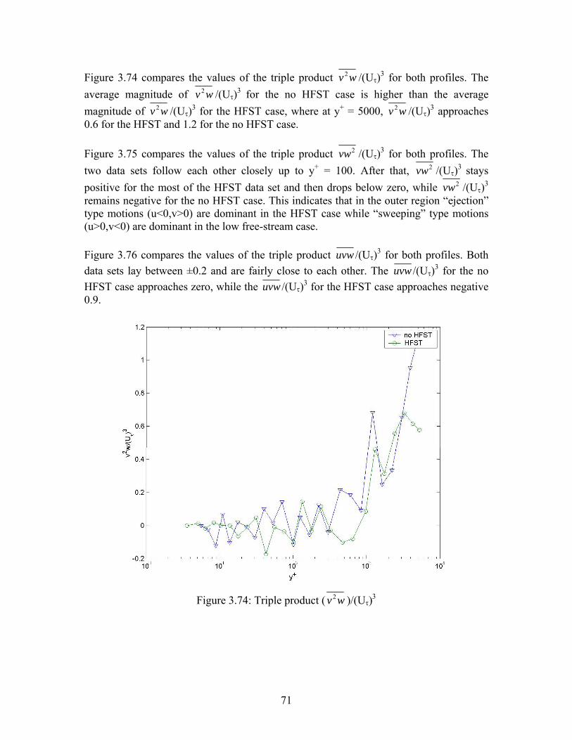
Figure 3.74 compares the values of the triple product wv 2 /(Uτ)3 for both profiles. The average magnitude of wv 2 /(Uτ)3 for the no HFST case is higher than the average magnitude of wv 2 /(Uτ)3 for the HFST case, where at y+ = 5000, wv 2 /(Uτ)3 approaches 0.6 for the HFST and 1.2 for the no HFST case. Figure 3.75 compares the values of the triple product 2vw /(Uτ)3 for both profiles. The two data sets follow each other closely up to y+ = 100. After that, 2vw /(Uτ)3 stays positive for the most of the HFST data set and then drops below zero, while 2vw /(Uτ)3

remains negative for the no HFST case. This indicates that in the outer region “ejection” type motions (u<0,v>0) are dominant in the HFST case while “sweeping” type motions (u>0,v<0) are dominant in the low free-stream case. Figure 3.76 compares the values of the triple product uvw /(Uτ)3 for both profiles. Both data sets lay between ±0.2 and are fairly close to each other. The uvw /(Uτ)3 for the no HFST case approaches zero, while the uvw /(Uτ)3 for the HFST case approaches negative 0.9.

Figure 3.74: Triple product ( wv 2 )/(Uτ)3

71

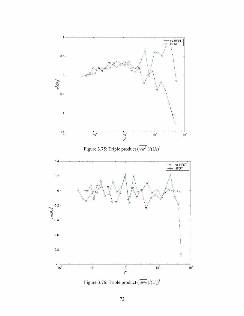
Figure 3.75: Triple product ( 2vw )/(Uτ)3

Figure 3.76: Triple product (uvw )/(Uτ)3

72

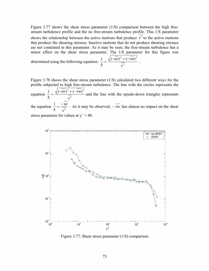
Figure 3.77 shows the shear stress parameter (1/S) comparison between the high free-stream turbulence profile and the no free-stream turbulence profile. This 1/S parameter shows the relationship between the active motions that produce 2v to the active motions that produce the shearing stresses. Inactive motions that do not produce shearing stresses are not contained in this parameter. As it may be seen, the free-stream turbulence has a minor effect on the shear stress parameter. The 1/S parameter for this figure was

determined using the following equation: 2

22 )()(1v

vwuvS

−+−= .

Figure 3.78 shows the shear stress parameter (1/S) calculated two different ways for the profile subjected to high free-stream turbulence. The line with the circles represents the

equation 2

22 )()(1v

vwuvS

−+−= and the line with the upside-down triangles represents

the equation 2

1vuv

S−

= . As it may be observed, vw− has almost no impact on the shear

stress parameter for values at y+ > 40.

Figure 3.77: Shear stress parameter (1/S) comparison

73

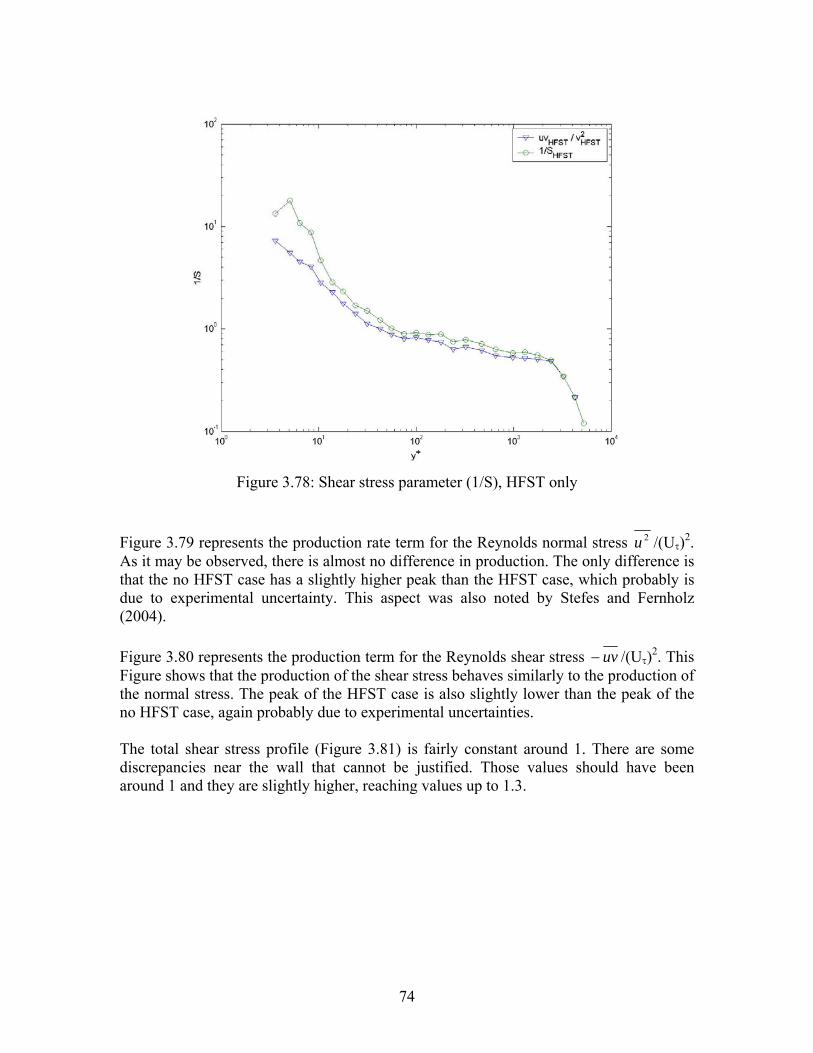
Figure 3.78: Shear stress parameter (1/S), HFST only

Figure 3.79 represents the production rate term for the Reynolds normal stress 2u /(Uτ)2. As it may be observed, there is almost no difference in production. The only difference is that the no HFST case has a slightly higher peak than the HFST case, which probably is due to experimental uncertainty. This aspect was also noted by Stefes and Fernholz (2004). Figure 3.80 represents the production term for the Reynolds shear stress uv− /(Uτ)2. This Figure shows that the production of the shear stress behaves similarly to the production of the normal stress. The peak of the HFST case is also slightly lower than the peak of the no HFST case, again probably due to experimental uncertainties. The total shear stress profile (Figure 3.81) is fairly constant around 1. There are some discrepancies near the wall that cannot be justified. Those values should have been around 1 and they are slightly higher, reaching values up to 1.3.

74

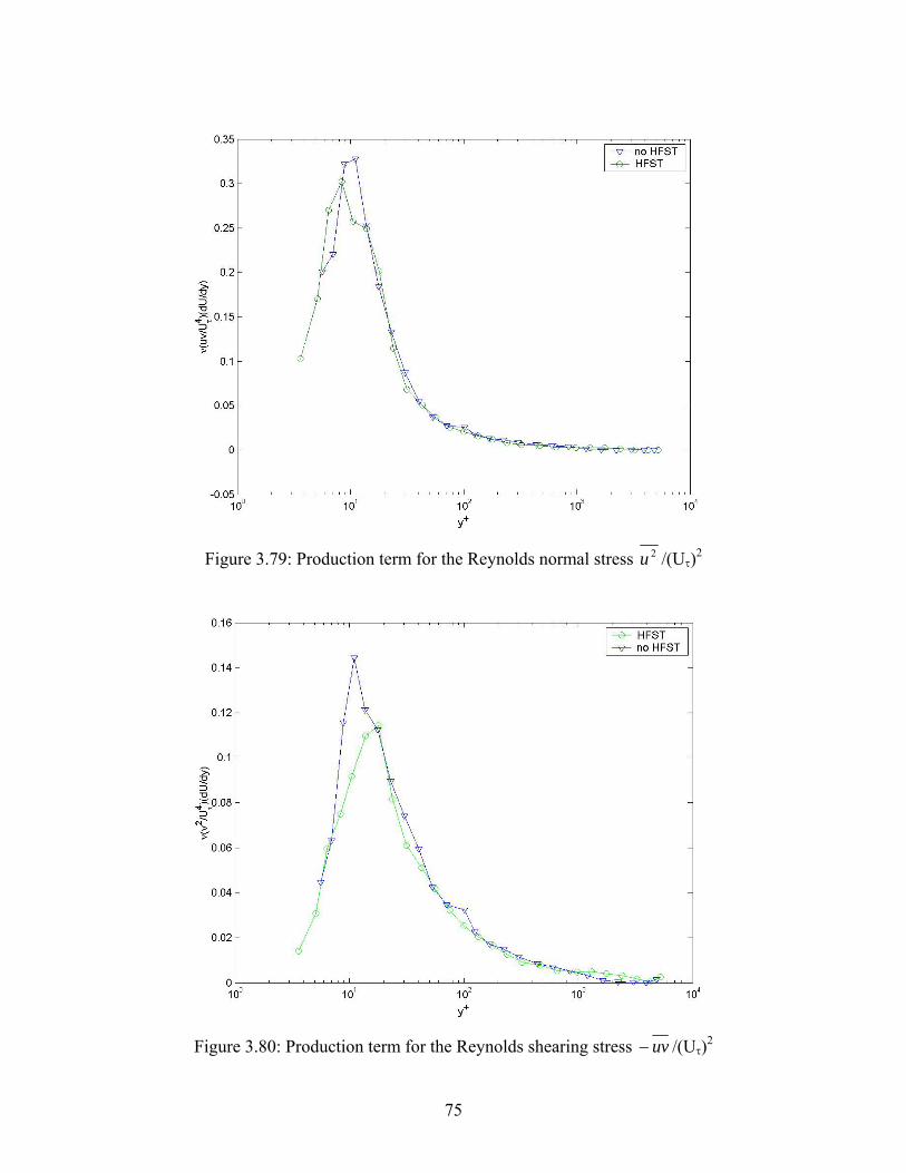
Figure 3.79: Production term for the Reynolds normal stress 2u /(Uτ)2

Figure 3.80: Production term for the Reynolds shearing stress uv− /(Uτ)2

75

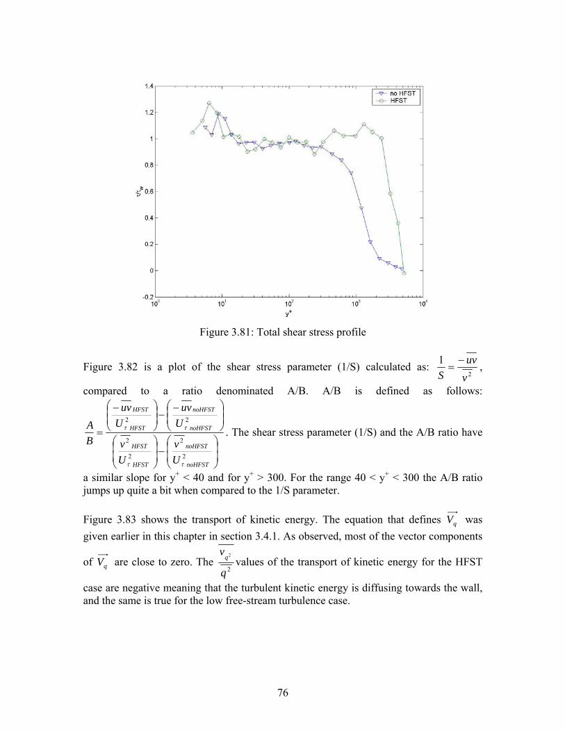
Figure 3.81: Total shear stress profile

Figure 3.82 is a plot of the shear stress parameter (1/S) calculated as: 2

1vuv

S−

= ,

compared to a ratio denominated A/B. A/B is defined as follows:

⎟⎟⎠

⎞⎜⎜⎝

⎛−⎟

⎟⎠

⎞⎜⎜⎝

⎛

⎟⎟⎠

⎞⎜⎜⎝

⎛ −−⎟⎟

⎠

⎞⎜⎜⎝

⎛ −

=

noHFST

noHFST

HFST

HFST

noHFST

noHFST

HFST

HFST

Uv

Uv

Uuv

Uuv

BA

2

2

2

2

22

ττ

ττ . The shear stress parameter (1/S) and the A/B ratio have

a similar slope for y+ < 40 and for y+ > 300. For the range 40 < y+ < 300 the A/B ratio jumps up quite a bit when compared to the 1/S parameter.

Figure 3.83 shows the transport of kinetic energy. The equation that defines qV was given earlier in this chapter in section 3.4.1. As observed, most of the vector components

of qV are close to zero. The 2

2

q

vq values of the transport of kinetic energy for the HFST

case are negative meaning that the turbulent kinetic energy is diffusing towards the wall, and the same is true for the low free-stream turbulence case.

76

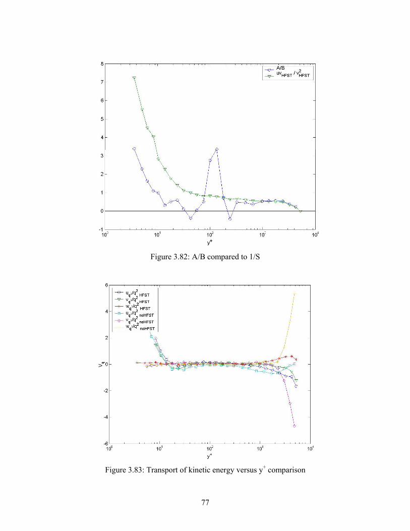
Figure 3.82: A/B compared to 1/S

Figure 3.83: Transport of kinetic energy versus y+ comparison

77

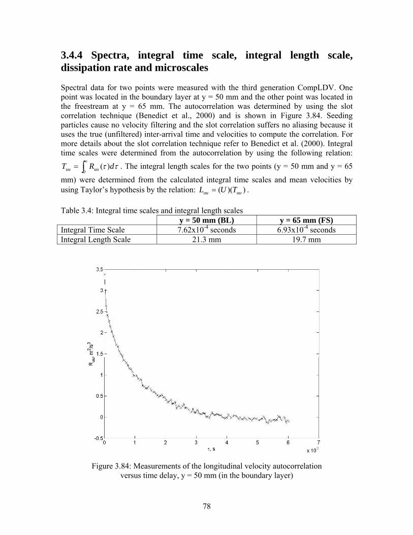
3.4.4 Spectra, integral time scale, integral length scale, dissipation rate and microscales

Spectral data for two points were measured with the third generation CompLDV. One point was located in the boundary layer at y = 50 mm and the other point was located in the freestream at y = 65 mm. The autocorrelation was determined by using the slot correlation technique (Benedict et al., 2000) and is shown in Figure 3.84. Seeding particles cause no velocity filtering and the slot correlation suffers no aliasing because it uses the true (unfiltered) inter-arrival time and velocities to compute the correlation. For more details about the slot correlation technique refer to Benedict et al. (2000). Integral time scales were determined from the autocorrelation by using the following relation:

. The integral length scales for the two points (y = 50 mm and y = 65

mm) were determined from the calculated integral time scales and mean velocities by using Taylor’s hypothesis by the relation:

∫∞

=0

)( ττ dRT uuuu

))(( uuuu TUL = . Table 3.4: Integral time scales and integral length scales y = 50 mm (BL) y = 65 mm (FS) Integral Time Scale 7.62x10-4 seconds 6.93x10-4 seconds Integral Length Scale 21.3 mm 19.7 mm

Figure 3.84: Measurements of the longitudinal velocity autocorrelation

versus time delay, y = 50 mm (in the boundary layer)

78

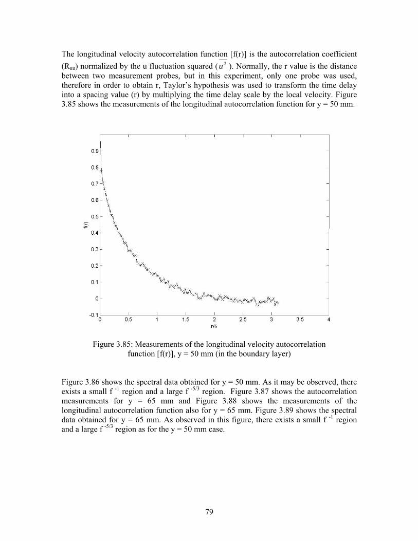
The longitudinal velocity autocorrelation function [f(r)] is the autocorrelation coefficient (Ruu) normalized by the u fluctuation squared ( 2u ). Normally, the r value is the distance between two measurement probes, but in this experiment, only one probe was used, therefore in order to obtain r, Taylor’s hypothesis was used to transform the time delay into a spacing value (r) by multiplying the time delay scale by the local velocity. Figure 3.85 shows the measurements of the longitudinal autocorrelation function for y = 50 mm.

Figure 3.85: Measurements of the longitudinal velocity autocorrelation

function [f(r)], y = 50 mm (in the boundary layer)

Figure 3.86 shows the spectral data obtained for y = 50 mm. As it may be observed, there exists a small f -1 region and a large f -5/3 region. Figure 3.87 shows the autocorrelation measurements for y = 65 mm and Figure 3.88 shows the measurements of the longitudinal autocorrelation function also for y = 65 mm. Figure 3.89 shows the spectral data obtained for y = 65 mm. As observed in this figure, there exists a small f -1 region and a large f -5/3 region as for the y = 50 mm case.

79

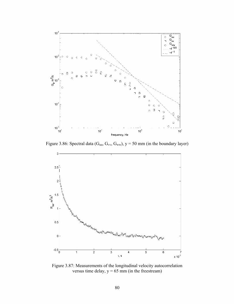
Figure 3.86: Spectral data (Guu, Gvv, Gww), y = 50 mm (in the boundary layer)

Figure 3.87: Measurements of the longitudinal velocity autocorrelation

versus time delay, y = 65 mm (in the freestream)

80

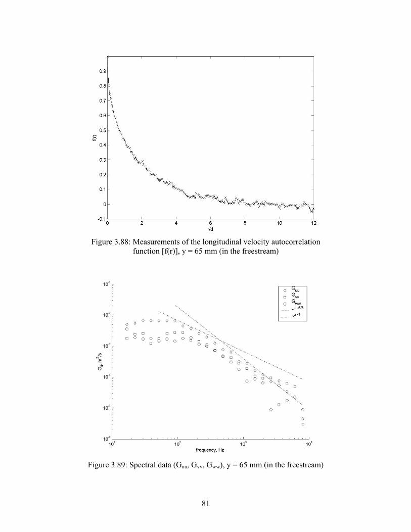
Figure 3.88: Measurements of the longitudinal velocity autocorrelation

function [f(r)], y = 65 mm (in the freestream)

Figure 3.89: Spectral data (Guu, Gvv, Gww), y = 65 mm (in the freestream)

81

Two model spectra were used to analyze the measured spectral data. The models used were the Pope’s model spectrum and the von Kármán’s model spectrum. For more details refer to Pope (2000, pp. 232-235). Both models used the same equations that are presented below, but with different variables. Some of these variables were obtained from Pope (2000) and other variables were calculated with equations that are shown below. The model for the energy-spectrum function is given by equation 3.3. According to Pope (2000) C = 1.5 and Cη = 0.40. And according to Saddoughi and Veeravalli (1994) β = 5.2.

)()()( 35

32

κηκκεκ ηfLfCE L

−= (3.3)

where oP

L

LCL

LLf

+

⎟⎟

⎠

⎞

⎜⎜

⎝

⎛

+=

35

212 ])[(

)(κ

κκ and }}]){[(exp{ 4144

ηηη κηβ ccf −+−=

Equation 3.4 is Pope’s (2000) equation 6.250, which is only valid for high Reynolds numbers. The integral in this equation is used to obtain CL for each model spectrum being studied here. For the Pope’s model spectrum, Po in equation 3.3 is equal to 2 and equal to 4 for the von Kármán’s model spectrum.

∫∞ −

=0

35

32

)()()()( LdLfkLLCq L κκε (3.4)

The following set of calculations was used to determine CL for the Pope’s model spectrum using Po = 2:

∫∫∞

+

−∞ −

⎟⎟

⎠

⎞

⎜⎜

⎝

⎛

+=

0

235

212

35

03

5)(

])[()()()()( Ld

CL

LLLdLfkLL

L κκ

κκκκ

If κL = x then:

∫ ∫∫∞

0

∞ ∞−−

⎟⎟

⎠

⎞

⎜⎜

⎝

⎛

+=⎟

⎟

⎠

⎞

⎜⎜

⎝

⎛

+=⎟

⎟

⎠

⎞

⎜⎜

⎝

⎛

+ 0 0 6112

2311

212

35

311

212

35

])[(])[()()(

])[()( dx

Cx

xdxCx

xxLdCL

LLLLL

κκ

κκ

31

31

0 6112

2

262.1

23

655

313

])[(

−−∞⋅≈

⎟⎠⎞

⎜⎝⎛Γ⎟

⎠⎞

⎜⎝⎛Γ

⎟⎠⎞

⎜⎝⎛Γ

=⎟⎟

⎠

⎞

⎜⎜

⎝

⎛

+∫ LL

L

CCdxCx

x

82

⎟⎠⎞⎜

⎝⎛ ⋅=

−3

1262.11

LCC

substituting C = 1.5, then CL = 6.783 for the Pope’s model spectrum.

The following set of calculations was used to determine CL for the von Kármán’s model spectrum using Po = 4:

∫∫∞

+

−∞ −

⎟⎟

⎠

⎞

⎜⎜

⎝

⎛

+=

0

435

212

35

03

5)(

])[()()()()( Ld

CL

LLLdLfkLL

L κκ

κκκκ

If κL = x then

∫ ∫∫∞

0

∞ ∞−−

⎟⎟

⎠

⎞

⎜⎜

⎝

⎛

+=⎟

⎟

⎠

⎞

⎜⎜

⎝

⎛

+=⎟

⎟

⎠

⎞

⎜⎜

⎝

⎛

+ 0 0 6172

4317

212

35

317

212

35

])[(])[()()(

])[()( dx

Cx

xdxCx

xxLdCL

LLLLL

κκ

κκ

5.111

6178

313

])[(3

1

0 6112

2

==⎟⎠⎞

⎜⎝⎛Γ

⎟⎠⎞

⎜⎝⎛Γ

=⎟⎟

⎠

⎞

⎜⎜

⎝

⎛

+

−∞

∫ CCdx

Cx

xL

L

π

715.35.1

1

6178

313

31

=→=⎟⎠⎞

⎜⎝⎛Γ

⎟⎠⎞

⎜⎝⎛Γ

−

LL CCπ

for the von Kármán’s model spectrum

Figure 3.90 and Figure 3.92 show the measurements of one-dimensional longitudinal velocity spectra compared to the Pope’s model spectrum at y = 50 mm (located in the boundary layer) and y = 65 mm (located in the freestream) respectively. Figure 3.91 and Figure 3.93 show the measurements of one-dimensional longitudinal velocity spectra compared to the von Kármán’s model spectrum at y = 50 mm (located in the boundary layer) and y = 65 mm (located in the freestream) respectively. By observing these four figures, it looks like the von Kármán model spectrum fits the spectral data better than the Pope’s model spectrum, specially for the spectral data at y = 50 mm (in the boundary layer). Also, the correlation coefficient between the spectral data and Pope’s spectrum, and the correlation coefficient between the spectral data and the von Kármán spectrum were determined. At y = 65 mm, the correlation coefficient between the spectral data and the Pope’s spectrum was equal to 0.9969, while the correlation coefficient between the spectral data and the von Kármán spectrum was equal to 0.9986. At y = 50 mm, the correlation coefficient between the spectral data and the Pope’s spectrum was equal to 0.9875, while the correlation coefficient between the spectral data and the von Kármán

83

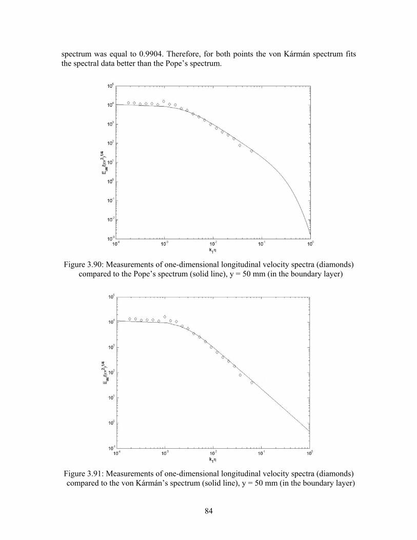
spectrum was equal to 0.9904. Therefore, for both points the von Kármán spectrum fits the spectral data better than the Pope’s spectrum.

Figure 3.90: Measurements of one-dimensional longitudinal velocity spectra (diamonds)

compared to the Pope’s spectrum (solid line), y = 50 mm (in the boundary layer)

Figure 3.91: Measurements of one-dimensional longitudinal velocity spectra (diamonds) compared to the von Kármán’s spectrum (solid line), y = 50 mm (in the boundary layer)

84

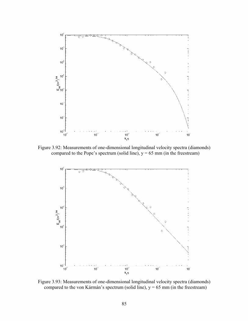
Figure 3.92: Measurements of one-dimensional longitudinal velocity spectra (diamonds)

compared to the Pope’s spectrum (solid line), y = 65 mm (in the freestream)

Figure 3.93: Measurements of one-dimensional longitudinal velocity spectra (diamonds)

compared to the von Kármán’s spectrum (solid line), y = 65 mm (in the freestream)

85

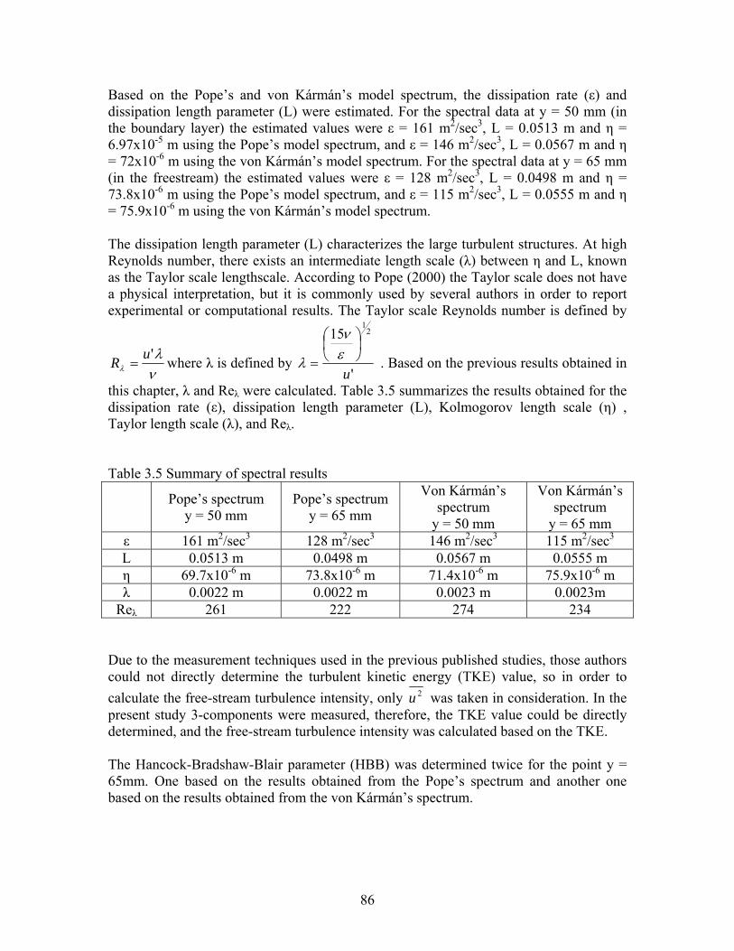
Based on the Pope’s and von Kármán’s model spectrum, the dissipation rate (ε) and dissipation length parameter (L) were estimated. For the spectral data at y = 50 mm (in the boundary layer) the estimated values were ε = 161 m2/sec3, L = 0.0513 m and η = 6.97x10-5 m using the Pope’s model spectrum, and ε = 146 m2/sec3, L = 0.0567 m and η = 72x10-6 m using the von Kármán’s model spectrum. For the spectral data at y = 65 mm (in the freestream) the estimated values were ε = 128 m2/sec3, L = 0.0498 m and η = 73.8x10-6 m using the Pope’s model spectrum, and ε = 115 m2/sec3, L = 0.0555 m and η = 75.9x10-6 m using the von Kármán’s model spectrum. The dissipation length parameter (L) characterizes the large turbulent structures. At high Reynolds number, there exists an intermediate length scale (λ) between η and L, known as the Taylor scale lengthscale. According to Pope (2000) the Taylor scale does not have a physical interpretation, but it is commonly used by several authors in order to report experimental or computational results. The Taylor scale Reynolds number is defined by

νλ

λ'uR = where λ is defined by

'

15 21

u

⎟⎠⎞

⎜⎝⎛

= εν

λ . Based on the previous results obtained in

this chapter, λ and Reλ were calculated. Table 3.5 summarizes the results obtained for the dissipation rate (ε), dissipation length parameter (L), Kolmogorov length scale (η) , Taylor length scale (λ), and Reλ. Table 3.5 Summary of spectral results

Pope’s spectrum y = 50 mm

Pope’s spectrum y = 65 mm

Von Kármán’s spectrum

y = 50 mm

Von Kármán’s spectrum

y = 65 mm ε 161 m2/sec3 128 m2/sec3 146 m2/sec3 115 m2/sec3

L 0.0513 m 0.0498 m 0.0567 m 0.0555 m η 69.7x10-6 m 73.8x10-6 m 71.4x10-6 m 75.9x10-6 m λ 0.0022 m 0.0022 m 0.0023 m 0.0023m

Reλ 261 222 274 234 Due to the measurement techniques used in the previous published studies, those authors could not directly determine the turbulent kinetic energy (TKE) value, so in order to calculate the free-stream turbulence intensity, only 2u was taken in consideration. In the present study 3-components were measured, therefore, the TKE value could be directly determined, and the free-stream turbulence intensity was calculated based on the TKE. The Hancock-Bradshaw-Blair parameter (HBB) was determined twice for the point y = 65mm. One based on the results obtained from the Pope’s spectrum and another one based on the results obtained from the von Kármán’s spectrum.

86

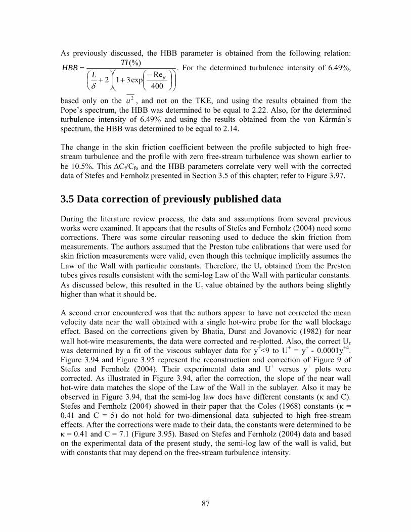
As previously discussed, the HBB parameter is obtained from the following relation:

⎟⎟⎠

⎞⎜⎜⎝

⎛⎟⎠⎞

⎜⎝⎛ −

+⎟⎠⎞

⎜⎝⎛ +

=

400Re

exp312

(%)

θ

δL

TIHBB . For the determined turbulence intensity of 6.49%,

based only on the 2u , and not on the TKE, and using the results obtained from the Pope’s spectrum, the HBB was determined to be equal to 2.22. Also, for the determined turbulence intensity of 6.49% and using the results obtained from the von Kármán’s spectrum, the HBB was determined to be equal to 2.14. The change in the skin friction coefficient between the profile subjected to high free-stream turbulence and the profile with zero free-stream turbulence was shown earlier to be 10.5%. This ∆Cf/Cfo and the HBB parameters correlate very well with the corrected data of Stefes and Fernholz presented in Section 3.5 of this chapter; refer to Figure 3.97. 3.5 Data correction of previously published data During the literature review process, the data and assumptions from several previous works were examined. It appears that the results of Stefes and Fernholz (2004) need some corrections. There was some circular reasoning used to deduce the skin friction from measurements. The authors assumed that the Preston tube calibrations that were used for skin friction measurements were valid, even though this technique implicitly assumes the Law of the Wall with particular constants. Therefore, the Uτ obtained from the Preston tubes gives results consistent with the semi-log Law of the Wall with particular constants. As discussed below, this resulted in the Uτ value obtained by the authors being slightly higher than what it should be. A second error encountered was that the authors appear to have not corrected the mean velocity data near the wall obtained with a single hot-wire probe for the wall blockage effect. Based on the corrections given by Bhatia, Durst and Jovanovic (1982) for near wall hot-wire measurements, the data were corrected and re-plotted. Also, the correct Uτ was determined by a fit of the viscous sublayer data for y+<9 to U+ = y+ - 0.0001y+4. Figure 3.94 and Figure 3.95 represent the reconstruction and correction of Figure 9 of Stefes and Fernholz (2004). Their experimental data and U+ versus y+ plots were corrected. As illustrated in Figure 3.94, after the correction, the slope of the near wall hot-wire data matches the slope of the Law of the Wall in the sublayer. Also it may be observed in Figure 3.94, that the semi-log law does have different constants (κ and C). Stefes and Fernholz (2004) showed in their paper that the Coles (1968) constants (κ = 0.41 and C = 5) do not hold for two-dimensional data subjected to high free-stream effects. After the corrections were made to their data, the constants were determined to be κ = 0.41 and C = 7.1 (Figure 3.95). Based on Stefes and Fernholz (2004) data and based on the experimental data of the present study, the semi-log law of the wall is valid, but with constants that may depend on the free-stream turbulence intensity.

87

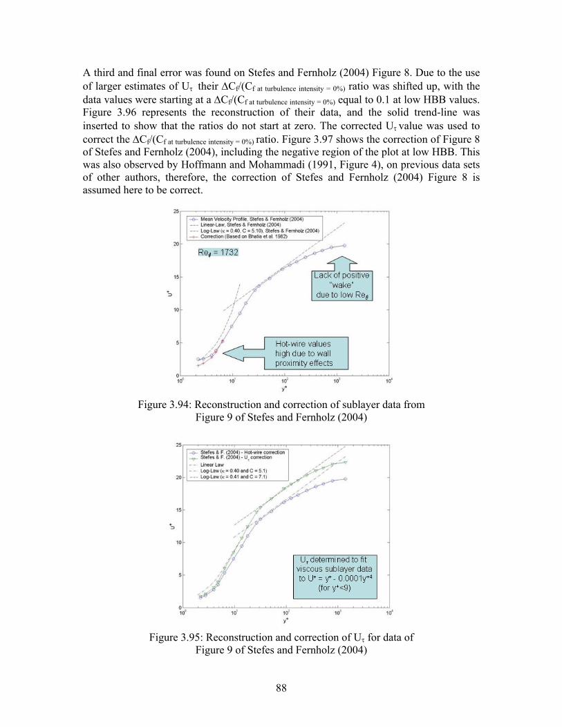
A third and final error was found on Stefes and Fernholz (2004) Figure 8. Due to the use of larger estimates of Uτ their ∆Cf/(Cf at turbulence intensity = 0%) ratio was shifted up, with the data values were starting at a ∆Cf/(Cf at turbulence intensity = 0%) equal to 0.1 at low HBB values. Figure 3.96 represents the reconstruction of their data, and the solid trend-line was inserted to show that the ratios do not start at zero. The corrected Uτ value was used to correct the ∆Cf/(Cf at turbulence intensity = 0%) ratio. Figure 3.97 shows the correction of Figure 8 of Stefes and Fernholz (2004), including the negative region of the plot at low HBB. This was also observed by Hoffmann and Mohammadi (1991, Figure 4), on previous data sets of other authors, therefore, the correction of Stefes and Fernholz (2004) Figure 8 is assumed here to be correct.

Figure 3.94: Reconstruction and correction of sublayer data from

Figure 9 of Stefes and Fernholz (2004)

Figure 3.95: Reconstruction and correction of Uτ for data of

Figure 9 of Stefes and Fernholz (2004)

88

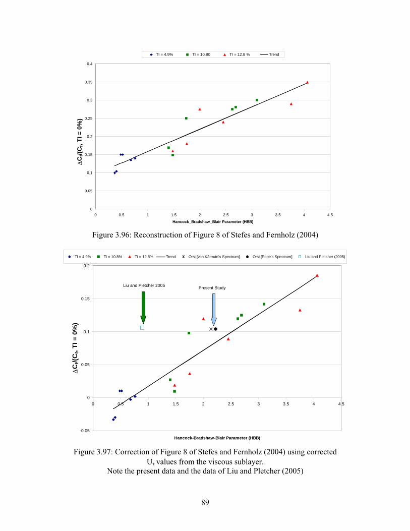
0

0.05

0.1

0.15

0.2

0.25

0.3

0.35

0.4

0 0.5 1 1.5 2 2.5 3 3.5 4 4

Hancock_Bradshaw_Blair Parameter (HBB)

∆C

f/(C

f, TI

= 0

%)

.5

TI = 4.9% TI = 10.80 TI = 12.8 % Trend

Figure 3.96: Reconstruction of Figure 8 of Stefes and Fernholz (2004)

-0.05

0

0.05

0.1

0.15

0.2

0 0.5 1 1.5 2 2.5 3 3.5 4 4

Hancock-Bradshaw-Blair Parameter (HBB)

∆C

f/(C

f, TI

= 0

%)

.5

TI = 4.9% TI = 10.8% TI = 12.8% Trend Orsi [von Kármán's Spectrum] Orsi [Pope's Spectrum] Liu and Pletcher (2005)

Present StudyLiu and Pletcher 2005

Figure 3.97: Correction of Figure 8 of Stefes and Fernholz (2004) using corrected

Uτ values from the viscous sublayer. Note the present data and the data of Liu and Pletcher (2005)

89

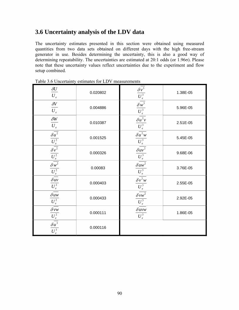
3.6 Uncertainty analysis of the LDV data The uncertainty estimates presented in this section were obtained using measured quantities from two data sets obtained on different days with the high free-stream generator in use. Besides determining the uncertainty, this is also a good way of determining repeatability. The uncertainties are estimated at 20:1 odds (or 1.96σ). Please note that these uncertainty values reflect uncertainties due to the experiment and flow setup combined. Table 3.6 Uncertainty estimates for LDV measurements

eUUδ 0.020802

3

3

eUvδ 1.38E-05

eUVδ 0.004886

3

3

eUwδ 5.96E-05

eUWδ 0.010387

3

2

eUvuδ 2.51E-05

2

2

eUuδ 0.001525

3

2

eUwuδ 5.45E-05

2

2

eUvδ 0.000326

3

2

eUuvδ 9.68E-06

2

2

eUwδ 0.00083

3

2

eUuwδ 3.76E-05

2eU

uvδ 0.000403 3

2

eUwvδ 2.55E-05

2eU

uwδ 0.000433 3

2

eUvwδ 2.92E-05

2eU

vwδ 0.000111 3eU

uvwδ 1.86E-05

3

3

eUuδ 0.000116

90

Chapter 4 Conclusions The objectives of this research project were to contribute to the expansion of the high free-stream turbulence database, to provide experimental data that will help on the improvement and validation of turbulence models, and to characterize the flow in the Aerospace and Ocean Engineering Boundary Layer Wind Tunnel with a high freestream turbulence (HFST) generator, which will be used in HFST studies around three-dimensional bodies. All work presented in this thesis was on nominally two-dimensional turbulent boundary layers at zero pressure gradient. High free-stream turbulence studies on three-dimensional boundary layers will be done in the future and may be found in Lowe (2006). The future three-dimensional study will simulate the flow around one turbine blade, where a wing/body junction (see Figure 1.2) will be used. The wing/body junction creates a three-dimensional pressure driven flow, which simulates exactly the flow around a turbine blade, which contains three-dimensional separation upstream of the blade and the formation of chaotic horseshoe vortex structures that wrap around the blade (Simpson, 2001). In order to satisfy the objectives, an active turbulence generator was used to create high free-stream turbulence in the boundary layer wind-tunnel, a seven-hole pressure probe was used to make mean velocity measurements, and a state of the art laser-Doppler velocimetry system was used to make mean and fluctuating velocity measurements. A turbulence intensity of 20% was desired, but the turbulence generator could not generate turbulent intensities higher than 7.9% due to limitations of the pressure regulator and air supply. During the turbulence generator’s testing phase, it was determined from the seven-hole pressure probe plane measurements, that the bottom row of jets (coflow and counterflow jets) of the turbulence generator were excessively speeding up the flow, making the boundary layer more three-dimensional. After some test cases, it was decided that the bottom row of coflow jets needed to have their diameters reduced by one half, and the bottom row of counterflow jets needed to be closed. In the region where the LDV measurements were made the spanwise variation of the mean velocity was less than 2%. For the first time, due to the technology available for this experiment, the skin friction coefficient (Cf) was deduced from the viscous sublayer, whereas in most of the previous published studies the authors assumed a semi-log layer with low free-stream turbulence constants to obtain the skin friction. The difference between the Uτ obtained in the viscous sublayer mean velocity profile and the Uτ obtained in the semi-log layer from

2τUuv =− was 1.5%.

Previous high free-stream turbulence studies were reviewed and discussed, where some of the previously published data of other authors have been corrected. Based on the measurements obtained with the LDV, the high free-stream turbulence was determined to

91

be nearly isotropic, and the turbulent kinetic energy was diffusing towards the wall. When a velocity profile subjected to no free-stream turbulence was compared to a

velocity profile subjected to high free-stream turbulence, it was observed based on 2

2

q

vq

that for both profiles the turbulent kinetic energy was diffusing towards the wall. The skin friction coefficient increased 10.5% due to the high free-stream turbulence and this change agrees with the data of Stefes and Fernholz (2004). It was also determined that the semi-log law of the wall is valid for high free-stream turbulence cases, but with different constants than the ones proposed by Coles (1968), where the constants for the high free-stream cases may be dependent on the turbulence intensity. For the present data, the constants were determined to be κ = 0.45 and C = 6.8. Spectral data obtained with the LDV, were compared to the von Kármán model spectrum and to the Pope’s model spectrum (Pope, 2000). Both model spectra fit the spectral data very well, but the von Kármán model spectrum had a higher correlation value with the spectral data than the Pope’s model spectrum. Finally, the ∆Cf/Cfo versus Hancock-Bradshaw-Blair parameter obtained for this experiment agreed very well with previously published data.

92

References Bangert, B.A; Kohli, A; Sauer, J.H. and Thole, K.A. 1997. “High freestream turbulence simulation in a scaled-up turbine vane passage.” ASME conference paper 97-GT-51. Benedict, L.H; Nobach, H. and Tropea, C. 2000. “Estimation of turbulent velocity spectra from laser Doppler data.” Measurement Science & Technology, Vol. 11, pp. 1089-1104. Bernero, Stefano. 2000a. “A turbulent jet in counterflow.” Doctor of Engineering Dissertation, Technische Universität Berlin, Berlin Germany. Bernero, Stefano and Fiedler, H.E. 2000b. “Application of particle image velocimetry and proper orthogonal decomposition to the study of a jet in a counterflow.” Experiments in Fluids, Vol. 29, no. 7, pp. S274-S281. Bhatia, J.C; Durst, F. and Jovanovic, J. 1982. “Corrections of hot-wire anemometer measurements near walls.” Journal of Fluid Mechanics, Vol. 122, September, pp. 411-431. Blair, M.F. 1983a. “Influence of free-stream turbulence on turbulence boundary layer heat transfer and mean profile development, Part I – experimental data.” Journal of Heat Transfer, Vol. 105, pp. 33-40. Blair, M.F. 1983b. ““Influence of free-stream turbulence on turbulence boundary layer heat transfer and mean profile development, Part II – analysis of results.” Journal of Heat Transfer, Vol. 105, pp. 41-47. Bonnin, J.C; Buchal, T. and Rodi, W. 1996. “ERCOFTAC Workshop on Data Bases and Testing of Calculation Methods for Turbulent Flows,” ERCOFTAC Bulletin 28, March. Bott, Donald M. and Bradshaw, Peter. 1998. “Effect of high free-stream turbulence on boundary-layer skin friction and heat transfer.” AIAA paper # 1998-531. Byun, Gwibo; Ölçmen, Semih M. and Simpson, Roger L. 2004. “A miniature laser-Doppler velocimeter for simultaneous three-velocity-component measurements.” Measurement Science and Technology, Vol. 15, pp. 2075-2082. Coles, D.E. and Hirst, E.A. 1968. “Proceedings computation of turbulent boundary layers, AFOSR-IFP-Stanford Conference”. Volume II, compiled data. Cousteix, J. and Houdeville, R. 1988. “The effects of unsteadiness on turbulent boundary layers.” Von Kármán Institute Lecture Series, April 18-22. Devenport, William J. and Simpson, Roger L. 1990. “Time-dependent and time-averaged turbulence structure near the nose of a wing-body junction.” Journal of Fluid Mechanics, Vol. 210, pp. 23-55.

93

Durst, F; Martinuzzi, R; Sender, J. And Thevenin, D. 1992. “LDA-measurements of mean velocity, rms-values and higher order moments of turbulence intensity fluctuations in flow fields with strong velocity gradients.” Sixth International Symposium on Applications of Laser Techniques to Fluid Mechanics, Lisbon, Portugal. Graf, Will and Simpson, Roger L. 2003. “Turbulence generator design.” Internal report. Virginia Polytechnic Institute and State University, Aerospace and Ocean Engineering Department, Blacksburg, Virginia. George, Jacob. 2005. “Structure of 2-D and 3-D turbulent boundary layers with sparsely distributed roughness elements.” Ph.D. Dissertation, Virginia Polytechnic Institute and State University, Aerospace and Ocean Engineering Department, Blacksburg, Virginia. Ha, Siew-Mun and Simpson, Roger L. 1993. “An experimental investigation of a three-dimensional turbulent boundary layer using multiple-sensor probes.” Proceedings of the ninth symposium on “Turbulent Shear Flows”. Kyoto, Japan, pp. 2-3-1 thru 2-3-6. Hancock, P. and Bradshaw, P. 1989. “Turbulence structure of a boundary layer beneath a turbulent free stream.” Journal of Fluid Mechanics, Vol. 205, pp. 45-76. Hancock, P. and Bradshaw, P. 1983. “The effect of free-stream turbulence on turbulent boundary layers.” ASME Journal of Fluids Engineering, Vol. 105, pp. 284-289. Hinze, J.O. 1975. “Turbulence”, Second Edition, McGraw-Hill Series in Mechanical Engineering, ISBN 0-07-029037-7. Hoffmann, J.A. and Mohammadi, K. 1991. “Velocity profiles for turbulence boundary layers under freestream turbulence.” Journal of Fluids Engineering, Vol. 113, pp 399-404. Hollingsworth, D.K. and Bourgogne, H.-A. 1995. “The development of a turbulent boundary layer in high free-stream turbulence produced by a two-stream mixing layer.” Experimental Thermal and Fluid Science, Vol. 11, pp. 210-222. Hunt, J.C.R. and Graham, J.M.R. 1978. “Free-stream turbulence near plane boundaries.” Journal of Fluid Mechanics, Vol. 84, part 2, pp. 209-235. Hussain, Fazle A.K.M. 1986. “Coherent structures and turbulence”. Journal of Fluid Mechanics, Vol. 173, pp.303-356. Kuhl, D.D. and Simpson, R.L. 2000. “Near-wall investigation of embedded streamwise vortex pairs.” Tenth International Symposium on Applications of Laser Techniques to Fluid Mechanics, Lisbon, Portugal. Liu, Kunlun and Pletcher, Richard H. 2005. “Large eddy simulation of turbulent boundary layers subjected to free-stream turbulence.” AIAA paper # 2005-669.

94

Lowe, K. Todd. 2006. “Design and application of an advanced Laser Doppler Velocimeter for high-order measurements in turbulent boundary layers.” Ph.D. Dissertation, Virginia Polytechnic Institute and State University, Aerospace and Ocean Engineering Department, Blacksburg, Virginia. Lowe, K. Todd and Simpson, Roger L. 2005. “Measurements of velocity-acceleration statistics in turbulent boundary layers.” TSFP-4, 4th International Symposium on Turbulence and Shear Flow Phenomena, Williamsburg – Virginia, paper # 186. Ölçmen, Semih M. and Simpson, Roger L. 1990. “An experimental study of a three-dimensional pressure-driven turbulent boundary layer.” Ph.D. Dissertation, Virginia Polytechnic Institute and State University, Aerospace and Ocean Engineering Department, Blacksburg, Virginia. Ölçmen, Semih M. and Simpson, Roger L. 1995. “An experimental study of a three-dimensional pressure-driven turbulent boundary layer.” Journal of Fluid Mechanics, Vol. 290, pp. 225-262. Pisterman, Kevin. 2004. “Use of a seven-hole pressure probe in highly turbulent flow-fields.” Master’s thesis, Virginia Polytechnic Institute and State University, Aerospace and Ocean Engineering Department, Blacksburg, Virginia. Pope, Stephen B. 2000. “Turbulent Flows.” Cambridge University Press, New York, NY, USA. Radomsky, R.W. and Thole, K.A. 1998. “Effects of high freestream turbulence levels and length scales on stator vane heat transfer.” ASME conference paper 98-GT-236. Rizzi, A. and Vos, J. 1998 “Toward Establishing Credibility in Computational Fluid Dynamic Simulations,” AIAA Journal, Vol. 36, no. 5, pp. 668-675. Saddoughi, S.G. and Veeravalli, S.V. 1994. “Local isotropy in turbulent boundary layers at high Reynolds number.” Journal of Fluid Mechanics, Vol. 268, pp. 333-372. Simpson, Roger L. 1973. “Turbulent Shear Flow - AOE 6154 Notes”. Virginia Polytechnic Institute and State University, Aerospace and Ocean Engineering Department, Blacksburg, Virginia. Simpson, R.L. 2001. “Junction Flows,” Annual Review of Fluid Mechanics, Vol. 33, pp. 415 – 441. Stefes, B. and Fernholz, H.-H. 2004. “Skin friction and turbulence measurements in a boundary layer with zero-pressure-gradient under the influence of high intensity free-stream turbulence.” European Journal of Mechanics B/Fluids, Vol. 23, pp. 303-318.

95

Stewart, Devin O. 2005. “The effects of spacing and geometry of three-dimensional distributed roughness elements on a two-dimensional turbulent boundary layer.” Master’s thesis, Virginia Polytechnic Institute and State University, Aerospace and Ocean Engineering Department, Blacksburg, Virginia. Thole, K. and Bogard, D. 1996. “High freestream turbulence effects on turbulent boundary layers.” ASME Journal of Fluids Engineering, Vol. 118, pp. 276-284. Thole, K; Bogard, D. and Whan, J. 1994. “Generating high freestream turbulence levels.” Experiments in Fluids, Vol. 17, pp. 375-380. Yoda, M. and Fiedler, H.E. 1996. “The round jet in a uniform counterflow: flow visualization and mean concentration measurements.” Experiments in Fluids, Vol. 21, pp. 427-436.

96

Vita Edgar Orsi Filho was born and raised in São Paulo, Brazil. In the fall of 1998, he decided to come to the United States to start his Aerospace Engineering and Computer Engineering careers at Embry-Riddle Aeronautical University in Prescott, Arizona. In the spring of 2003 Edgar graduated cum laude with a Bachelor of Science in Aerospace Engineering and a Bachelor of Science in Computer Engineering. He was also the outstanding Computer Engineering student of the Class of 2003. In the fall of 2003, he joined the Aerospace and Ocean Engineering Department at Virginia Polytechnic Institute and State University (Virginia Tech) in Blacksburg, Virginia in order to pursuit a higher education. He concluded his work in December of 2005 and graduated with a Master of Science degree in Aerospace Engineering.

97