an explanation of anomalous behavior in models in political participation

8/18/2019 An Explanation of Anomalous Behavior in Models in Political Participation

http://slidepdf.com/reader/full/an-explanation-of-anomalous-behavior-in-models-in-political-participation 1/13

American Political Science Review Vol. 99, No. 2 May 2005

An Explanation of Anomalous Behavior in Modelsof Political ParticipationJACOB K. GOEREE California Institute of Technology

CHARLES A. HOLT University of Virginia

T his paper characterizes behavior with “noisy” decision making for models of political interaction

characterized by simultaneous binary decisions. Applications include: voting participation games,candidate entry, the volunteer’s dilemma, and collective action problems with a contribution

threshold. A simple graphical device is used to derive comparative statics and other theoretical propertiesof a “quantal response” equilibrium, and the resulting predictions are compared with Nash equilibriathat arise in the limiting case of no noise. Many anomalous data patterns in laboratory experiments basedon these games can be explained in this manner.

Many political and social decisions involve onlytwo options: to vote or not, to enter a con-test or not, to join an alliance or not, etc. The

apparent simplicity of these binary-choice situations issomewhat misleading in that the best decision requirescorrect beliefs about others’ behavior. For instance,people may hesitate to go to a particular restaurant orbar when many others are likely to go, or as Yogi Berrasaid, “Nobody goes there anymore. It’s too crowded.”1

In other cases, the rewards associated with each deci-sion may be contingent on getting a minimal numberof decisions of a certain type, e.g., the choice by a coun-try of whether or not to join an alliance, or jump intoworld war, or impose an embargo. A similar exampleoccurs when a majority vote is needed to approve alegislative pay raise that each legislator would prefernot to support if it would pass otherwise (Ordeshook1986, chap 3). Sometimes the minimal number of con-tributors needed is only one, as in the “volunteer’s

dilemma,” where all players are better off if at least oneof them incurs a cost from vetoing an option, attempt-ing a dangerous rescue, or volunteering to perform atask that benefits them all (Diekmann 1985).

In all these examples, the question is whether inde-pendent choices made by different people will some-how generate the “correct” amount of participation orwhether the inability to coordinate will lead to defi-ciencies such as excess entry or crowding, insufficienteffortto produce a public good, or the failure of anyoneto initiate an action that benefits all. Another interest-ing issue is how aggregate behavior patterns respond

Jacob K. Goeree is Professor, Division of the Humanities and So-cial Sciences, California Institute of Technology, Mail Code 228-77, Pasadena, CA 91125 ([email protected]). Charles A. Holt isProfessor, Department of Economics, P.O. Box 400182, Universityof Virginia, Charlottesville, VA 22904-4182 ([email protected] [email protected]).

We gratefully acknowledge financial support from the NationalScience Foundation (SBR-0094800), the Alfred P. Sloan Foundation,the Bankard Fund at the University of Virginia, and the Dutch Na-tional Science Foundation (VICI 453.03.606). This paper benefitedfrom comments provided by three anonymous referees, RebeccaMorton, Howard Rosenthal,and participants at the quantal responseworkshop at Caltech and the politics seminar at NYU.1 Entry decisions in this context are known as the “El Farol”dilemma, named after a popular bar in Santa Fe (Morgan, Bell,and Sethares 1999).

to changes in the number of people involved and therelevant costs and benefits of participation.

This paper is motivated in part by the surprising andsometimes anomalous behavior patterns observed inmany laboratory experiments that involve simple bi-nary choices. For example, Kahneman (1988) reportsan experiment in which the number of people who de-cide to enter was approximately equal to a “capacity”parameter that determined whether or not entry wasprofitable. He remark, “To a psychologist, it looks likemagic.” Subsequent experiments have been based onsimilar models, and the general finding is that play-ers are able to coordinate entry decisions in a man-ner that roughly equates expected profits for entry tothe opportunity cost (Ochs 1990; Sundali, Rapoport,and Seale 1995).2 However, the “magic” of efficiententry coordination has been called into question byrecent experimental results. For example, Fischbacherand Th ¨ oni (2001) conducted an experiment in which

a monetary prize is awarded to a randomly selectedentrant, so the expected prize amount is a decreasingfunction of the number of entrants. Over-entry wasobserved, and it was more severe for larger numbers of potential entrants. This over-entry pattern is somewhatintuitive but contradicts the theoretical prediction thatrewards should be equalized for the two options, inde-pendent of the number of potential entrants. Camererand Lovallo (1999) also find over-entry when posten-try payoffs depend on a skill-based competition, butthey report under -entry and positive net payoffs in theabsence of such competition.

Other interesting behavior patterns have beenobserved in experiments based on the volunteer’s

dilemma, in which everyone receives a benefit if at least one person incurs the cost of “volunteering” buteach person would prefer to free-ride on others’ ef-forts. The theoretical prediction is that an increase inthe number of potential volunteers will reduce theprobability that any one person volunteers, which isintuitive, and will decrease the probability that at least one person volunteers, which is unintuitive. Experi-mental data support the intuitive prediction but not theunintuitive one (Franzen 1995). Similarly, laboratory

2 This successfulcoordination has been explained by models of adap-tation and learning (Erev and Rapoport 1998; Meyer et al. 1992).

201



Anomalous Behavior in Models of Political Participation May 2005

results for binary coordination games and collectiveaction problems support some theoretical predictions,but also generate intuitive data patterns that are notexplained by standard game theory, as discussed below.

The objective of this paper is to explore the commonstructural elements of a wide class of binary-choicegames, and to provide a unified theoretical perspectiveon seemingly contradictory results, like the positive re-

lationship between over-entry (or the probability of getting a volunteer) and the number of potential en-trants (or volunteers). Our approach involves relax-ing the extreme rational choice assumption of perfectmaximizing behavior where people respond sharply tosmall payoff differences, which, in reality, are likelyto be dwarfed by an array of emotions, perceptionbiases, and unobserved individual differences in fair-mindedness, altruism, etc. Instead of trying to model allthese dimensions explicitly, our approach is to replacethe knife-edge responses to small payoff differenceswith “smoothed” stochastic responses that representrandom variations in unobserved factors (Goeree andHolt 1999; McKelvey and Palfrey 1995; Palfrey and

Rosenthal 1985, 1988). The broader value of this workis that it provides an enriched and empirically usefulgame theory that applies to the kinds of situations of concern to political scientists, i.e., those with a richdiversity of individual motivations and attitudes. Inaddition, we derive our results using a simple graphicaldevice that can be used in a wide variety of seeminglyunrelated binary-choice situations.

TO PARTICIPATE OR NOT?

A symmetric N -person participation game is charac-terized by two decisions, which we call participate and

exit.3

Examples include the decision of whether ornot to run for office, try to unseat an incumbent, orapproach a wealthy donor seeking campaign contribu-tions. The payoff from participation is a function of the total number, n, who decide to participate, whichis denoted π(n), defined for n≤N . In a campaign entrygame, for example, the payoff for all candidates may bea decreasing function of the number, n, who enter. Theexpected payoff for the exit decision is denoted c(n),which is typically nondecreasing in n (the number of players that enter). In many applications, c(n) is simplya constant that can be thought of as the opportunitycost of participation, but we keep the more generalnotation to include examples where a higher number

of participants has external benefits to all, includingthose who do not participate (e.g., campaigning forcivil rights; see Chong 1991).

A strategy in this game is a participation probability, p ∈ [0, 1]. In order to characterize a symmetric equi-librium, consider one player’s decision when all othersparticipate with probability p. Since a player’s own pay-off is a function of the number who actually participate,

3 The participation game terminology wasintroduced by Palfrey andRosenthal (1983) in the context of the decision of whether or notto vote. This model is discussed below, under Voting ParticipationGames.

the expected payoff for participation is a function of thenumber of other players, N − 1, and the probability pthat any one of them will participate. Assuming in-dependence, the distribution of the number of otherparticipants is binomial, with parameters N − 1 and p. This distribution, together with the underlying π(n)function, can be used to calculate the expected partici-pation payoff, which is denoted πe( p, N − 1). More

precisely, πe

( p, N − 1) is defined to be the expectedpayoff if a player participates (with probability 1) whenall N − 1 others participate with probability p. Simi-larly, ce( p, N − 1) is the expected payoff from exitwhen the N − 1 others participate with probability p.

Equilibrium

In a Nash equilibrium, players choose the decision thatyields the highest expected payoff, or randomize in thecase of indifference. Our goal is the explanation of “anomalous” data from laboratory experiments, so itis convenient to model a type of noisy behavior thatincludes the rational-choice Nash predictions as a limitcase. One way to relax the assumption of noise-free,perfectly rational behavior is to specify a utility func-tion with a stochastic component. For example, peoplemay be motivated to vote by a sense of citizen duty(Riker and Ordeshook 1968), the strength of whichmay vary across individuals and across time for thesame individual as external factors change. Thus theexpected payoff for participation, πe, and the expectedpayoff for exit, ce, are each augmented by adding thestochastic term µεi, where µ > 0 is an “error” param-eter and the εi represent identically and independentlydistributed realizations of a random variable for deci-sion i = 1 (participate) or 2 (exit). The utility of partic-

ipation is greater if πe

+ µε1 > ce

+ µε2, so that whenµ = 0 the decision with the highest expected payoff is selected, but higher values of µ imply more noiserelative to payoff maximization. This noise can be dueeither to errors (e.g., distractions, perception biases,or miscalculations that lead to nonoptimal decisions)or to unobserved utility shocks that make rational be-havior look noisy to an outside observer. Regardlessof the source, the result is that choice is stochastic,and the distribution of the random variable determinesthe form of the choice probabilities.4 The participationdecision is selected if πe + µε1 > ce + µε2 or, equiv-alently, if ε2 − ε1 < (πe − ce)/µ, which occurs withprobability

p = F

πe( p, N − 1) − ce( p, N − 1)

µ

, (1)

where F is the distribution function of the differenceε2 − ε1. Since the two random errors are identicallydistributed, the distribution of their difference willbe “symmetric” around 0, so F (0) = 1/2.5 The error

4 For instance, a normal distribution yields the probit model, while adoubleexponentialdistribution gives rise to thelogitmodel, in whichcase the choice probabilities are proportional exponential functionsof expected payoffs.5 More formally, Pr(ε1 ≤ ε2)= 1/2, so Pr(ε1 − ε2 ≤ 0)=F (0) = 1/2.

202



American Political Science Review Vol. 99, No. 2

parameter, µ, determines the responsiveness of partic-ipation probabilities to expected payoffs. Perfectly ran-dom behavior (i.e., p = 1/2) results as µ →∞, sincethe argument of the F ( · ) function on the right side of Eq. (1) goes to zero and F (0) = 1/2 as noted above.Perfect rationality results in the limit as µ → 0, sincethe choice probability converges to zero or one, de-pending on whether the expected participation payoff

is less than or greater than the expected exit payoff.More generally, for µ > 0, Eq. (1) expresses the par-ticipation probability as a noisy best response to theexpected-payoff-difference, which we also refer to as a“stochastic best response.”

Equation (1) characterizes a quantal response equi-librium (McKelvey and Palfrey 1995) if the participa-tion probability p in theexpected payoffexpressions onthe right is equal to the choice probability that emergeson the left.6 Without further parametric assumptions,there is no closed-form solution for the equilibriumparticipation probability, but a simple graphical devicecan be used to derive theoretical properties and char-acterize factors that might cause systematic deviations

from Nash predictions. The graph is based on a separa-tion of the expected-payoff-difference from a term thatdepends only on thenoiseelements (µ and the distribu-tion of random elements). To this end, apply theinverseof the F function to both sides of (1) and multiply by µ

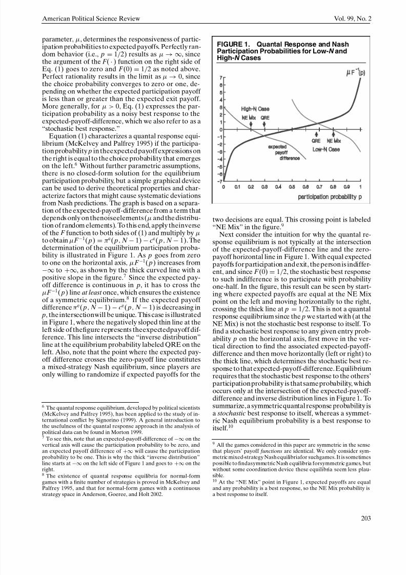
to obtain µF −1( p) = πe( p, N − 1) − ce( p, N − 1). Thedetermination of the equilibrium participation proba-bility is illustrated in Figure 1. As p goes from zeroto one on the horizontal axis, µF −1( p) increases from−∞ to +∞, as shown by the thick curved line with apositive slope in the figure.7 Since the expected pay-off difference is continuous in p, it has to cross theµF −1( p) line at least once, which ensures the existence

of a symmetric equilibrium.8

If the expected payoff difference πe( p, N − 1) − ce( p, N − 1) is decreasing in p, the intersectionwill be unique. This case is illustratedin Figure 1, where the negatively sloped thin line at theleft side of thefigure represents theexpectedpayoff dif-ference. This line intersects the “inverse distribution”line at the equilibrium probability labeled QRE on theleft. Also, note that the point where the expected pay-off difference crosses the zero-payoff line constitutesa mixed-strategy Nash equilibrium, since players areonly willing to randomize if expected payoffs for the

6 The quantal response equilibrium, developed by political scientists(McKelvey and Palfrey 1995), has been applied to the study of in-ternational conflict by Signorino (1999). A general introduction tothe usefulness of the quantal response approach in the analysis of political data can be found in Morton 1999.7 To see this, note that an expected-payoff-difference of −∞ on thevertical axis will cause the participation probability to be zero, andan expected payoff difference of +∞ will cause the participationprobability to be one. This is why the thick “inverse distribution”line starts at −∞ on the left side of Figure 1 and goes to +∞ on theright.8 The existence of quantal response equilibria for normal-formgames with a finite number of strategies is proved in McKelvey andPalfrey 1995, and that for normal-form games with a continuousstrategy space in Anderson, Goeree, and Holt 2002.

FIGURE 1. Quantal Response and NashParticipation Probabilities for Low-N andHigh-N Cases

two decisions are equal. This crossing point is labeled“NE Mix” in the figure.9

Next consider the intuition for why the quantal re-sponse equilibrium is not typically at the intersectionof the expected-payoff-difference line and the zero-payoff horizontal line in Figure 1. With equal expectedpayoffs for participation and exit, the person is indiffer-ent, and since F (0) = 1/2, the stochastic best responseto such indifference is to participate with probabilityone-half. In the figure, this result can be seen by start-ing where expected payoffs are equal at the NE Mix

point on the left and moving horizontally to the right,crossing the thick line at p = 1/2. This is not a quantalresponse equilibrium since the p we started with (at theNE Mix) is not the stochastic best response to itself. Tofind a stochastic best response to any given entry prob-ability p on the horizontal axis, first move in the ver-tical direction to find the associated expected-payoff-difference and then move horizontally (left or right) tothe thick line, which determines the stochastic best re-sponse to thatexpected-payoff-difference. Equilibriumrequires that the stochastic best response to the others’participationprobability is thatsameprobability, whichoccurs only at the intersection of the expected-payoff-difference and inverse distribution lines in Figure 1. Tosummarize, a symmetricquantal response probability isa stochastic best response to itself, whereas a symmet-ric Nash equilibrium probability is a best response toitself.10

9 All the games considered in this paper are symmetric in the sensethat players’ payoff functions are identical. We only consider sym-metric mixed-strategy Nash equilibriafor suchgames. It is sometimespossible to findasymmetric Nash equilibria forsymmetric games, butwithout some coordination device these equilibria seem less plau-sible.10 At the “NE Mix” point in Figure 1, expected payoffs are equaland any probability is a best response, so the NE Mix probability isa best response to itself.

203




As long as the expected payoff difference is decreas-ing in p, it is apparent from Figure 1 that any factorthat increases the expected payoff difference line forall values of p will move the intersection with the thickinverse distribution line to the right and, hence, raisethe quantal response equilibrium probability. In anentry game, for example, the original π(n) functionwould be decreasing if expected rewards are decreasing

in the number of entrants, and it is then straightfor-ward to show that πe(N − 1, p) is a decreasing func-tion of both arguments.11 When the opportunity costpayoff from not entering is constant, it follows thatthe expected-payoff-difference πe( p, N − 1) − ce( p,

N − 1) is decreasing in p and N , so a reduction in thenumber of potential entrants will shift the thin linein the figure upward and raise the quantal response(QRE) probability, as represented by a comparison of the high-N case on the left with the low-N case on theright.

The effect of additional “noise” in this model is easilyrepresented, since an increase in the error parameter µ

makes the µF −1( p) line steeper around the midpoint, p = 1/2, although it still passesthrough the zero-payoff line at this midpoint (see Figure 1). This increase innoise, therefore, moves the quantal response equilib-rium closer to one-half, as would be expected. In con-trast, as a reductionin µ makes the µF −1( p) line flatter,and in the limit it converges to the horizontal line atzero as the noise vanishes. In this case, the crossingsfor the QRE and mixed Nash equilibria match up, aswould be expected.

Next, consider coordination-type games where par-ticipation can be interpreted as an individual decisionof whether or not to help with a group productionprocess that will only succeed if enough people help

out. For example, participation in revolutionary activi-ties may be individually costly unless the movementreaches a critical mass. In such games, it does not payto participate unless enough others do, so π(n) willbe less than c(n) for low n and greater than c(n) forhigh n. Thus the right side of Eq. (1) is increasing inthe probability of participation. This property may re-sult in multiple quantal response equilibria since therecan be multiple intersections when both the expected-payoff-difference and the inverse distribution lines areincreasing in p (see Figure 2, which shows a case with

11 Intuitively, holding N fixed, a higherprobability of entering meansthat more people enter, which results in a lower expected payoff

of entry. Similarly, holding p fixed, a higher number of potentialentrants results in more entry. This can be made more precise asfollows: suppose N is fixed and the entry probability is p 1. Let thenumberof entrants be determined by drawing a randomnumber thatis uniformly distributed on [0, 1] for each player. If the number is lessthan p 1, a player enters; otherwise the player stays out. When theprobability of entering increases to p2 > p 1, the number of entrantsis at least thesameas beforefor allpossible realizationsof therandomvariables, and greaterfor somerealizations. (When a player’s randomvariable is less than p1, it is certainly less than p 2, leading to thesame entry decision, and when it lies between p1 and p2, the player’sdecision changes from staying out to entering.) Likewise, when p isfixed, an increase in the potential number of entrants means thatfor all possible realizations of players’ random draws, the numberof entrants is the same or higher, which makes the expected payoff from entry the same or lower.

FIGURE 2. Quantal Response and NashMixed Participation Probabilities for a Gamewith Positive Externalities

three intersections). With multiple crossings, any fac-tor that shifts the expected-payoff-difference line up-ward will move some intersection points to the leftand others to the right. Thus the comparative staticseffects are of opposite signs at adjacent equilibria, andwe need to use an analysis of dynamic adjustmentto restrict consideration to equilibria that are stable(the Samuelsonian “correspondence principle”).12 Asimple dynamic model can be based on the intuitiveidea that the participation probability will increaseover time when the “noisy best response” to a given

p is higher than p. Thus d p/dt > 0 when F ((πe( p, N −1) − ce( p, N − 1))/µ) > p , or equivalently, p wouldtend to increase when πe( p, N − 1) − ce( p, N − 1) >µF −1( p) and decrease otherwise. For example, startat p = .6 in Figure 2, which gives a positive expected-payoff-difference and a stochastic best response of al-most .9, found by moving horizontally to the right. Forthis reason, a rightward arrow is present at p = .6 onthe horizontal axis. The other directional arrows arefound similarly, so there is an unstable QRE at about.3, with arrows pointing away. In this manner it can beseen that the quantal response equilibrium will be sta-ble whenever the expected-payoff-difference line cutsthe inverse distribution line from above.

Note that any factor that raises the payoff fromparticipation, and hence shifts the expected-payoff-difference line upward in Figure 2, will raise the QREparticipation probability if the equilibrium is stable andnot otherwise. To summarize:

Proposition 1. There is at least one symmetric quan-tal response equilibrium in a symmetric binary-choice participation game. The equilibrium is unique if the difference between the expected payoff of participating and

12 Similar dynamic-stability arguments were used by Palfrey andRosenthal (1988) and Fey (1997).

204




that of exiting is decreasing in the probability of participation. In this case, any exogenous factor that increasesthe participation payoff or lowers the exit payoff will raisethe equilibriumparticipation probability. The samecomparative statics result holds when there are multipleequilibria and attention is restricted to stable equilibria.

It is useful to begin with a discussion of entry gamessince they are the simplest application. Moreover, thequantal response properties for these games also ap-ply to the stable equilibria in more complex applica-tions such as threshold contribution games, volunteer’sdilemma, and voting. The reader who is primarily in-terested in one of these subsequent applications maywish to skip any of the later sections after reading asfar as Proposition 2.

ENTRY GAMES: UNDER-ENTRY ANDOVER-ENTRY RELATIVE TO MIXEDNASH PREDICTIONS

A widely studied example that fits the binary-choice

framework is an “entry” game, where the choice isbetween a risky entry decision with high potential pay-offs (if few others enter) and a secure exit payoff. Forexample, entry may correspond to launching a politicalcampaign or filing an application for a limited num-ber of public broadcast licenses. There are N potentialentrants, and we assume that if all others enter withprobability one, the representative player would pre-fer to exit due to congestion, but if nobody else enters,then the player would prefer to enter: πe(1, N − 1) <

ce(1, N − 1) and πe(0, N − 1) > ce(0, N − 1). Considera simple three-person congestion problem where eachperson’s payoff from participation is one unless bothothers also participate, in which case congestion re-duces the payoff to zero. The exit payoff is c, with0 < c < 1. When both others participate with probabil-ity p, theprobability of congestionis p2, so πe = 1− p2,which is less than the exit payoff c when p = 1 andgreater than the exit payoff when p = 0. In this ex-ample and in all other applications considered below,the expected-payoff-difference will be continuous anddecreasing in p, so there is a unique p∗ for which

πe( p∗, N − 1) = ce( p∗, N − 1). (2)

[For instance, in the three-person congestion prob-lem p∗ = (1− c)1/2.] Since (2) implies indifference,it characterizes the unique symmetric Nash equilib-

rium in mixed strategies. The net payoff for participa-tion, πe( p, N − 1) − ce( p, N − 1), is decreasing in p, asshown by the “expected-payoff-difference” line on theleft in Figure 1. As noted above, the crossing of thisthin line and the horizontal line at zero represents thesolution to Eq. (2) and is labeled “NE Mix” on the leftside of the figure.

In order to compare the Nash and quantal responseequilibria, note that the thin lines representing thedifferences in expected payoffs are always negativelysloped in an entry game. First, consider the high-N case on the left, where the large number of potentialentrants lowers the expected payoff associated with a

given participation probability, and the resulting mixedequilibrium is less than one-half. The intersection of thenegatively sloped thin line and the increasing inversedistribution line determines the quantal response par-ticipation probability, and this intersection will be tothe right of the mixed Nash probability. The oppositeoccurs for the low-N case on the right side of the graph,where the low number of potential entrants results in a

mixed equilibrium that is greater than one-half. In thislow-N case, the QRE probability is biased downwardfrom theNash probability. One way to understand bothcases is to note that the effect of adding noise is to pushthe equilibrium toward one-half.13

Finally, recall that the thin lines in Figure 1 repre-sent the expected-payoff-difference on the right side of Eq. (1). At the QRE probability on the left, net ex-pected payoffs are negative and there is over-entry inthis case of a high number of potential entrants. Incontrast, the thin line lies above the zero line at theQRE probability on the right side, for the low-N case.This negative relationship between the number of po-tential entrants andthe net returns from participationis

consistent with the experimental results of Fischbacherand Th ¨ oni (2001) discussed in the Introduction.14 Tosummarize:

Proposition 2. In the quantal response equilibrium for the entry game, there is over-entry resulting in negativenet expected payoffs when the mixed-strategy Nash equi-librium is less than one-half. The reverse effect , under-entry, occurswhen the mixed Nash equilibrium is greater than one-half.

The implication of Proposition 2 is that the quantalresponse equilibrium for the entry game is always be-tween the Nash equilibrium and one-half. Therefore,

an observed participation that is more extreme thanthe Nash prediction would contradict the quantal re-sponse equilibrium model for any error rate, µ, andany distribution of stochastic shocks, F .

Meyer et al. (1992) report an experiment in whichsubjects choose to enter one of two markets. With agroup size of six, profits are equalized, with three ineach market, so the equilibrium probability of entryis one-half. An immediate corollary to Proposition 2is that in this case QRE coincides with Nash and bothpredict an entry probability of one-half. This predictionis borne out by their data: the average of the numberof people that enter each market is never statistically

different from three in the 11 baseline sessions that

13 In some games with strong strategic interactions, the “snowball”effects of small amounts of noise can push decisions away from theunique Nash equilibrium so strongly that they overshoot the mid-point of the strategy space, with most of the theoretical density atthe opposite end of the set of feasible decisions from the Nash pre-diction. This is the case for some parameterizations of the “traveler’sdilemma” (Capra et al. 1999). This prediction, that the data will beclustered on the opposite side of the midpoint decision from theNash equilibrium, is borne out by the experimental evidence.14 In their game, a prize worth V is awarded randomly to one of then players who purchase a lottery ticket at cost c, so π(n) = (V /n) − c.From this it can be shown that the expected-payoff-difference isdecreasing in p and N .

205




they report (see their Table 3), even when the game isrepeated for as many as 60 periods (see their Table 5).15

Camerer and Lovallo (1999) provide support for theQRE under-entry prediction when the Nash probabil-ity of entry is greater than one-half. In their experimentsubjects decide whether or not to enter a contest with afixed number, c, of prizes. The entrants were randomlyranked and the top c entrants divide $50 according

to their rank, while all other entrants lose $10. Theexit payoff is simply 0, and the equilibrium number of entrants is (close to)c + 5. The parameters werechosensuch that the Nash entry probability was greater thanor equal to one-half in all treatments.16 Under-entryoccurred in all of the eight sessions in their baselinetreatment, which resulted in positive expected payoffsfor entry (see their Table 4). The net expected payoff of entry across sessions and periods was $15, whichtranslates into under-entry of one or two subjects perround.17

The strongest evidence for the quantal responsepredictions in Proposition 2 can be found in Sundali,Rapoport, and Seale 1995. In their experiments, subjects received a fixed payoff of one for exit and anentry payoff that is increasing in market capacity,c, and decreasing in the number of entrants: π(n) =1 + 2(c − n). Thus entry in excess of capacity reducespayoffs below one, the payoff for exit. It is straight-forward to derive the mixed Nash entry probability: p∗ = (c − 1)/(N − 1), which is approximately equalto the ratio of capacity to number of potential en-trants.18 The capacities for the various treatments werec = 1, 3, . . . , 19, and with groups of N = 20 subjects,the Nash equilibrium probability ranged from p ∗ = 0to p∗ = 18/19. Figure 3 shows the entry decisions av-eraged over all subjects, with the Nash predictions

15 Meyer et al.(1992)also reportsome evidence that does notsquarewith either the symmetric Nash or the quantal response predictionsof our model. In particular, the frequency with which subjects switchmarkets is lower than the predicted frequency (50%). We conjecturethat this “inertia” could be explained by an asymmetric quantal re-sponse equilibrium in which some people tend to enter with higherprobability than others.16 The number of prizes was either 2, 4, 6, or 8, yielding equilibriumnumbers of entrants (c+ 5) of 7, 9, 11, or 13 respectively, which arealways greater than or equal to half the group size (14–16).17 Camerer and Lovallo (1992) also report a second treatment inwhich subjects are told beforehand that their performance on sportsor current events trivia will determine their payoff. This creates aselection bias, since people that participate in the experiment aremore likely to think they will rank high when they enter (i.e., they

are “overconfident”),neglectingthe fact that otherparticipants thinkthe same (“reference group neglect”). Camerer and Lovallo proposeoverconfidence and reference groupneglect as a possibleexplanationof the over-entry that occurs in this second treatment. This explana-tion is quite plausible, in that it is analogous to the failure to perceivea selection bias that causes winners in a common-value auction tobe the ones who overestimated its value. Note that overconfidencecannot be the whole story, however, since this bias does not explainunder-entry in their baseline treatment.18 To derive this symmetric mixed equilibrium, note that the ex-pected number of other people who enter is (N − 1) p, so if a per-son enters, the expected total number of entrants is 1 + (N − 1) p.Then π(n) can be used to calculate the expected payoff for entering:πe( p, N − 1) = 1 + 2(c − 1) − (N − 1)2 p and the Nash equilibriumprobability of entering follows by equating this expected payoff tothe exit payoff of one, which yields the result in the text.

FIGURE 3. Nash Predictions (Solid Line) andObserved Entry Probabilities (Diamonds)(Source: Sundali, Rapoport, and Seale 1995)

shown as the 45◦ line. Since each subject participatedin 10 “runs” and there were three groups of 20 subjects, a data point in the figure is the average of 10 ∗ 3 ∗ 20 = 600 entry decisions. Note that the entryfrequency is generally higher than predicted by Nashfor p∗ < 1/2 and lower than predicted for p∗ > 1/2, inline with the quantal response equilibrium predictions.

To summarize, the quantal response analysis ex-plains the “magical” conformity to Nash entry predic-tions (e.g., Meyer et al. 1992), the under-entry in theCamerer andLovallo 1999 baseline, the over-entry withmany potential entrants observed by Fischbacher andTh ¨ oni (2001), and the systematic pattern of deviationsfrom Nash predictions reported by Sundali, Rapoport,andSeale (1995). Thisgeneral approachcan be adaptedto evaluate behavior in other contexts where payoffsforone decision arediminished as a resultof congestioneffects, as the next section illustrates.19

THE VOLUNTEER’S DILEMMA

There are many situations in which a player’s decisionto participate benefits others. In collective action prob-lems, for instance, the contributions of some have pos-itive returns for everyone involved, and these returns

are increasing in the number of contributors. In somecontexts, the critical number of participants is one, e.g.,

19 The analysis presented here does not apply directly to the ex-periments reported in Ochs 1990, since his experiments involvedmore than two market locations, each with a different “capacity”that determined thenumber of entrants that could be accommodatedprofitably. Nevertheless, the data patterns with random regrouping(“high turnover”) are suggestive of the quantal response results de-rived here. The locations with the most capacity (and high probabil-ities) consistently have a lower frequency of entry than required fora mixed-strategy Nash equilibrium, whereas the opposite tendencywas observed for locations with the capacity to accommodate onlyone entrant profitably.

206




TABLE 1. Frequencies of IndividualVolunteer Decisions (p ) and of “NoVolunteer” OutcomesN p P (No Volunteer )

2 .65 .123 .58 .075 .43 .067 .25 .13

9 .35 .0221 .30 .0051 .20 .00

101 .35 .00

Source : Franzen(1995).

when a volunteer is needed to issue a politically riskyveto or sanction a group member who violated a norm.The dilemma in these situations is that volunteeringis costly and players have an incentive to free ride onothers’ benevolence.

In the volunteer’s dilemma game studied here(Diekmann 1986), all players receive a benefit B if at least one of them incurs a cost, C < B. In this case,the expected payoff of participation, or “volunteer-ing,” is simply a constant, B− C . The expected pay-off from “exiting” follows from the observation thatwhen the N − 1 others volunteer with probability p,there is a (1 − p)N −1 chance that no one volunteers, soce( p, N − 1) = B(1 − (1− p)N −1). Note that the vol-unteer’sdilemmagamesatisfies the assumptionsunder-lying Figure 1, i.e., the difference between the expectedpayoff of participating and that of exiting is decreasingin p. The Nash probability of volunteering follows byequating these expected payoffs (as per Eq. [2]) toobtain

p∗ = 1 −

C

B

1N −1

. (3)

This probability of volunteering has the intuitive prop-erties that it is increasing in the benefit, B, decreas-ing in the cost, C , and decreasing in the number of potential volunteers, N . However, the probability of getting no volunteers is (1− p∗)N . By Eq. (3) theprobability of getting no volunteers in a Nash equi-librium is (C /B)N /(N −1), which is increasing in N , withlim N →∞P (No Volunteer)=C /B > 0. Unlike the in-tuitive comparative statics properties mentioned be-fore, this prediction is not supported by experimen-

tal data. Table 1 reports experimental results for aone-shot volunteer’s dilemma game with B = 100 andC = 50 (Franzen 1995). Note that the probability thatany person volunteers is generally declining with N ,as predicted by Nash.20 The probability that no onevolunteers, however, is decreasing in N and convergesto zero instead of C /B = 1/2.

Next, consider the quantal response equilibrium forthe volunteer’s dilemma. Since the difference betweenthe expected payoff of volunteering that of and exiting

20 Franzen (1995) reports that the group-size effect is significant atthe 5% level using a chi-square test with seven degrees of freedom.

is decreasing in the probability of volunteering, Propo-sition 1 implies that the QRE probability of volunteer-ing is unique, decreasing in N and C , and increasingin B. Interestingly, the introduction of (enough) en-dogenous noise reverses the unintuitive Nash predic-tion that the probability of “no volunteer” increaseswith N .

Proposition 3. In the quantal response equilibrium for the volunteer’s dilemma game, the probability that no one will volunteer is decreasing in the number of potential volunteers for a sufficiently high error rate,µ. Furthermore, limN →∞P(No Volunteer)= 0 for anyµ > 0.

The proof of Proposition 3 is given in the Appendix.The intuition is that, in the presence of noise, the ad-dition of potential volunteers only results in a smallreduction in the probability of volunteering, and thenet effect is that the chance that someone volunteerswill rise.21

The unintuitive feature of the Nash equilibrium for

the volunteer’s dilemma (i.e., that the probability of getting no volunteer increases with N ) parallels theresult that the chance of convicting an innocent de-fendant under the unanimity rule (i.e., no acquittalvotes) rises with the size of the jury (Feddersen andPesendorfer 1998). The models differ in that jurorsreceive private signals about the likelihood that thedefendant is guilty. In the Nash equilibrium, those thatreceive a guilty signal vote to convict while those withan innocentsignal randomize between voting to convictor to acquit. As the jury size increases, an individual juror’s propensity to vote to acquit with an innocentsignal falls, and the chance that there is not a singlevote to acquit rises. As a result, it becomes more likely

that an innocent defendant is wrongfully convicted(Feddersen and Pesendorfer 1998). In laboratory juryvoting experiments, subjects tend to vote strategicallyas predicted by the Nash equilibrium. However, theunintuitive numbers effect is not supported by experi-mental data and is not implied by a quantal responseequilibrium analysis (Guarnaschelli, McKelvey, andPalfrey 2000).

GAMES WITH MULTIPLE EQUILIBRIA:STEP-LEVEL PUBLIC GOODS GAMES

In some binary-choice games the expected payoff func-

tion for participating is not decreasing in p. For exam-ple, in any collective political activity where a criticalmass is required to achieve a desired outcome (e.g.,regime change), the net reward from participating willbe higher as others become more involved.22 There-fore, the payoff difference function is increasing in

21 In the extreme case when µ →∞, players volunteer with prob-ability one-half, irrespective of the number of potential volunteers,and the chance that no one volunteers falls exponentially, since theprobability of no volunteer is 2−N .22 In the discussion that follows we treat the threshold as a sharpcutoff even though it is more reasonable in most contexts to modelthethreshold as a range of participation over which theprobabilityof

207




the probability of participation, which permits mul-tiple crossings as shown in Figure 2. This is intuitive,since there may exist both low-participation equilib-ria and high-participation equilibria in such “coordi-nation” or “assurance” games.23 A particular exampleis a step-level public goods game, where N players de-cide whether or not to “contribute” at cost c. If thetotal number of contributions meets or exceeds some

threshold n∗

, then the public good is provided and allplayers receive a fixed return, V , whether nor not theycontributed. Here we assume that the contribution islike an effort that is lost if the threshold is not met,so there is “no rebate.” The threshold n∗ could corres-pond to a required number of participants in an em-bargo or signatures on a petition.24

In the standard linear public goods games without astep, observed contributions in experiments are posi-tively related to the marginal effectof a contribution onthe value of the public good, known as the marginal per capita return (MPCR).25 Anderson, Goeree, and Holt(1998) have shown that a logit quantal response anal-ysis predicts this widely observed MPCR effect. This

raises the question whether there is a similar measureor index that would predict the level of contributionsin step-level public goods games. One would intuitivelyexpect that contributions are positively related to thetotal (social) value of the public good (NV ) and nega-tively related to the minimum total cost of providing it(n∗c). Croson and Marks (2000) have proposed usingthe ratio ofsocial value tocost, which they call the “stepreturn:” SR = NV /n∗c. Based on a meta-analysis of several step-level public goods games, they conclude,“. . . Subjects respond to the step return just as theycorrespond to the marginal per capita return (MPCR)in linear public goods games: higher step returns lead

to more contributions.”First, we consider whether there is a clear theoret-ical basis for expecting contributions to be positivelyrelated to step return measures. A contribution in thisgame pays off only when it is pivotal, i.e., when exactlyn∗ − 1 others contribute, which happens with probabi-lity

N − 1n∗ − 1

pn∗−1(1− p)N −n∗ , (4)

where, as before, p denotes the probability that othersparticipate. The difference between the expectedpayoff of contributing and that of not contributing is

success is sharply increasing. The use of a sharp cutoff simplifies theanalysis and is standard in the literature (see, e.g., Lohmann 1994).23 Stability arguments can often be used to rule out the middleequilibrium if there are three crossings as in Figure 2. For low µ ,this middle equilibrium is usually close to a mixed Nash equilibriumwith “perverse” comparative statics properties. The high- and low-participation equilibria then correspond to low-effort and high-effortpure-strategy Nash equilibria that often arise in coordination games.24 Gilligan (2003) considers the problem of determining the “cor-rect” number of countries needed to ratify a treaty. A higher thresh-old indicating broader support typically requires a less restrictiveagreement.25 This literature is surveyed in Ostrom’s (1998) presidential addressto the American Political Science Association and in Miller 1997.

FIGURE 4. Expected-Payoff-Differences andthe Inverse Distribution Line for DifferentThresholds in Step-Level Public Goods Games

thereforeπe( p, N − 1) − ce( p, N − 1)

=V

N − 1n∗ − 1

pn∗−1(1− p)N −n∗ − c. (5)

The right side is a single-peaked function of p, andequating its derivative to zero yields a unique max-imum at p = (n∗ − 1)/(N − 1). Figure 4, drawn forV = 6, c = 1, and N = 10, shows these “hillshaped”expected-payoff-difference lines for three values of thethreshold: n∗ = 3, 5, 8. (Please ignore the “n∗ = {5, 8}”line, which pertains to a multiple-step case consideredlater.) In each case there are two Nash equilibria inmixed strategies, determined by the crossings of thethin line with the horizontal line at zero. The inversedistribution line is plotted for the case of a logisticdistribution, i.e., F ( x) = 1/(1+ exp(− x)), and µ = 1.As before, the intersection of the inverse distributionline with the thin lines determines the quantal responseequilibrium, which is unique for all three values of thethreshold in this numerical example.26

Recall that the step return is NV /n∗c, which is in-creasing in N and V and decreasing in n∗ and c. Inorder to evaluate these properties in the context of the quantal response predictions, note that the bell-shaped nature of the expected payoff differences im-

plies that there may be multiple quantal response equi-libria. It follows from Proposition 1, however, that anyfactor that shifts the expected payoff difference lineupward will raise the equilibrium probability in a stable

26 More generally, when the expected-payoff-difference line is in-creasing there may be multiple equilibria for some values of theerror rate µ. For instance, a slight upward shift in the “n∗ = 8” linein Figure 4 would result in three quantal response equilibria. Thestability analysis associated with Figure 2 can be used to show thatthe middle equilibrium is unstable; see also Fey 1997 and Palfreyand Rosenthal 1988. The likelihood of having multiple equilibriais increased when µ is small and the µF −1( p) line is essentiallyhorizontal for p between zero and one.

208




equilibrium. Since thedifference in Eq. (5)is increasingin V and decreasing in c, we conclude that the equi-librium contribution probability will be increasing inV and decreasing in c, just as indicated by the stepreturn effect. Next, consider the effect of the numbersvariables, N and n∗, beginning with a somewhat infor-mal graphical analysis (precise results are presentedin Proposition 4, below). Recall that the maximum of

the expected-payoff-difference “hill” is at a probabilityof (n∗ − 1)/(N − 1), so an increase in N tends to shiftthis function to the left. Note that a leftward shift inthe thin line labeled n∗ = 3 in Figure 4 will lower theequilibrium probability, but a slightleftward shift in theline labeled n∗ = 8 will move the intersection point upalong the thick line and, hence, will raise the quantalresponse equilibrium probability. Thus an increase in N can result in a decrease in the equilibrium probabilitywhen the threshold is low and an increase when thethreshold is high.27 The effects of changes in the thresh-old, n∗, are similar. Note that the quantal responseprobability of contributing does not decrease mono-tonically with the threshold: when n∗ increases from 3to 5, the equilibrium probability increases from .43 to.56, and then drops to .27 when n∗ = 8. The intuition isthat when the threshold rises and it is still likely that thepublic good will be provided, individual contributionswill rise, but contributions drop dramatically when toomany contributions are needed for provision. To sum-marize, in a quantal response equilibrium, a higher stepreturn ratio leads to more contributions when it is dueto a higher total value of the public good or a lowercost of provision, but not necessarily when it is due toan increase in the number of potential contributors orto a lower threshold. Thus the (admittedly theoretical)analysis here yields only qualifiedsupport forthe use of

the step return as a rough measure of the propensity tocontribute in a binary step-level public goods game.28

Of course, even when individual contributions risein response to the increased threshold, the probabilitythat the public good is actually provided may decrease,since more people are needed to meet the threshold.For the numeric example represented in Figure 4, theprobability of success drops from .83 to .62 to practi-cally zero when n∗ is increased from 3 to 5 to 8. vande Kragt, Orbell, and Dawes (1983) report an experi-ment that implemented a step-level public goods gamewith binary contributions and found that increasing thenumber of contributors needed for success reduced theincidence of successful provision. The next proposition

shows that these findings are in line with QRE predic-tions when there is sufficient noise.

27 See, for instance, Offerman, Schram, and Sonnemans 1997 forexperimental evidence on some of these comparative static results.28 Nor are the numbers effects in a Nash equilibrium necessarilyconsistent with the qualitative properties of the step return ratio.This is because an increase in the threshold n∗ shifts the maximumof the expected-payoff-difference line to the right in Figure 4, whichis likely to shift the rightmost (stable) mixed Nash equilibrium to theright. Thus a rise in n∗, which lowers the step return, can raise themixed Nash contribution probability.

FIGURE 5. QRE Probabilities of IndividualContribution and Successful Group Provisionof a Step-Level Public Good, as a Functionof the Provision Point

Proposition 4. For a high enough error rate, µ, thequantal response equilibrium for the step-level public goods game is unique and predicts that individual con-tributions first rise and then fall with the threshold, n∗,while the probability of successful provision always de-creases with n∗.

This proposition, which is proved in the Appendix,is illustrated in Figure 5, which was drawn for the casewhere V = 6, c = 1, N = 10, µ = 1.5, and with the pro-vision point, n∗, varying from 1 to 9. A movement tothe right in the figure corresponds to an increase in the

number of contributors needed for successful provi-sion, which reduces the probability of success in a quan-tal response equilibrium. As the step level is increased,individual contributions first increase to meet thechallenge and then fall as the threshold becomes moreunattainable. Interestingly, Palfrey and Rosenthal(1988) derive this result in an equivalent manner byintroducing random, individual-specific “joy of giving”(or “warm-glow” altruism) shocks that are added to aperson’s payoff for a contribution decision.29 Proposi-tion 4 extends their analysis by showing that the prob-ability of successful provision is decreasing in n∗.

Finally, it is interesting to see how contribution be-havior changes as multiple steps, or thresholds, are in-

troduced. Suppose, for instance, that in addition to then∗ = 5 threshold, there is another threshold at n∗ = 8:with five or more contributions, everyone receives areturn of one from the public good, while with eightcontributions or more, the return is two. This multiple-step case canbe analyzedin the same manner as before.

29 The Nash equilibrium for the resulting game of incomplete infor-mation is mathematically equivalent to a quantal response equilib-rium. Palfrey and Rosenthal (1988) prove that individual contribu-tions first rise and then fall with the threshold (see their Table 2).They also show that the number of potential contributors, N , has thereverse effect: individual contributions first fall and then rise withincreases in N .

209




Now there are two points at which one’s contributioncan bepivotal, and the expectedpayoff is the sum of thetwo effects. In terms of Figure 4, the expected payoff lines for n∗ = 5 and n∗ = 8 get “summed,” as indicatedby the n∗ = {5, 8} line in Figure 4 (the cost of con-tributing only enters once, which is why the endpointsof this are still at −1). The introduction of the extrathreshold at n∗ = 8, which by itself results in a low

contribution probability, dramatically increases contri-butions: the QRE contribution probability is .73 andthe probability that at least five people contribute is ashigh as .97. An immediate extension of this analysisis that adding more steps, without reducing the payoff increment at any of the existing steps, will increasequantal response contribution probabilities in a binarypublic goods game.

VOTING PARTICIPATION GAMES

Another binary choice of considerable interest is thedecision whether or not to vote in a small-group sit-uation where voting is costly and a single vote hasa nonnegligible effect on the final outcome, e.g., thedecision whether to attend a faculty meeting on a busyday. The analysis is similar to that of a step-level pub-lic goods game, since the threshold contribution, n∗,corresponds to the number of votes needed to pass afavored bill. In a real voting contest, however, the votetotal required to win is endogenously determined bythe number of people voting against the bill. If thereare two types of voters, those who favor a bill andthose who oppose, then the equilibrium will be char-acterized by a participation probability for each type.Here we restrict attention to a symmetric model withequal numbers of voters of each type, equal costs of

voting, c, and symmetric valuations: V if the preferredoutcome receives more votes and zero otherwise. Tiesin this majority rule game are decided by the flip of a coin. Note that the public goods incentives to free-ride are still present in this game, since voters benefitwhen their side wins, regardless of whether or not theyincurred the cost of voting.

The analysis of the majority voting game is a straight-forward application of the approach taken in the pre-vious sections. The gain from a favorable outcome is V ,so the expected-payoff-difference is V times the prob-ability that one’s vote affects the outcome minus thecost of voting. (Obviously, the net cost of voting couldbe small or even negative if voting is psychologicallyrewarding or if there are social pressures to vote, e.g.,to attend a faculty meeting.) Since a tie is decided bythe flip of a coin, the probability that a vote is piv-otal is one-half times the probability that it creates orbreaks a tie. In a symmetric equilibrium with commonparticipation probability, p, it is straightforward to usethe binomial formulas to calculate these probabilities,and the expected payoff difference for voting is thenV /2 times this “influence probability” minus the cost of voting.30

30 Suppose there are two groups of equal size, N , and consider aplayer in group 1. The player’s vote is pivotal only when the number

FIGURE 6. Nash and Quantal ResponseVoting Probabilities Under Majority andProportional Rules

Figure 6 shows the expected-payoff-difference asa function of the common participation probability,which is labeled “majority rule.” The parameters thatwere used to construct this figure are taken fromSchramand Sonnemans (1996b), whoconducted an ex-periment based on this game form with N = 6, V = 2.5,and c = 1. The “U” shape of the expected-payoff-difference reflects the fact that a costly vote is wastedwhen the preferred outcome is already winning orwhen it cannot win even with an extra vote. Indeed,the expected value of a vote is highest when either noone else or everyone else votes, since a vote is thenguaranteed to be pivotal by breaking or creating a tie.

In contrast, when all others vote with probability 1/2,one extra vote is likely to be superfluous or not enoughandits expected value is therefore small. As in previoussections, the mixed Nash prediction is determined bywhere the expected-payoff-difference line crosses thezero line: there are two Nash equilibria, one in whichalmost no one votes and another in which almost ev-eryone votes (Palfrey and Rosenthal 1983).

The quantal response equilibrium is determined bythe intersection of the expected-payoff-difference lineand the inverse distribution function (thick lines).31

of voters in group 1 is equal to n2 − 1 or n2, where n2 denotes thenumber of voters in group 2, which happens with probability

N n2=1

N n2

N − 1n2 − 1

p2n2−1(1− p)2N −2n2

+

N −1n2=0

N n2

N − 1

n2

p2n2 (1 − p)2N −2n2−1,

where, as before, p denotes the probability with which all others (inboth groups) vote. The first term represents the probability that a tieis created and the second term is the probability that a tie is broken.A player’s expected payoff is V /2 times this “influence probability”minus c, the cost of voting.31 Palfrey and Rosenthal (1985) use essentially the same techniquesto determine the Bayesian–Nash equilibrium in a voting game with

210




The µ parameter of .8 used to construct the steeperline was selected so that the QRE prediction wouldbe at about the same level (30% to 50%) as the voteparticipation probabilities reported by Schram andSonnemans (1996b) in the initial periods of their ex-periment. Interestingly, the voting probabilities startedhigh and then decreased to stabilize somewhere in the20% to 30% range. This downward trend is crudely

captured by a reduction in the noise parameter µ to .4as indicated by the second inverse distribution line inFigure 6.32

Schram and Sonnemans (1996b) also considered a“proportional rule” game in which the payoff for allparticipants is the proportion of votes for their pre-ferred outcome, minus the cost of voting if they voted.Again, it is straightforward to use the binomial for-mula to calculate the expected proportion of favorablevotes, contingent on one’s own decision of whetherto vote, as a function of the common participationprobability, p.33 The expected payoff difference forthis proportional representation game is the increasein the expected proportion of favorable votes, minus

the cost of voting. This difference is declining every-where because one’s vote has a smaller impact on thevote proportion as the probability of others’ participa-tion increases. The expected-payoff-difference line islabeled “proportional rule” in Figure 6, where the pa-rameters are again taken from Schram and Sonnemans(1996b): N = 6, V = 2.22, and c = 0.7. The Schram andSonnemans data for the proportional rule experiments,plotted as the lower line in Figure 7, started in the 30%to 40% range and ended up between 20% and 30%in the final periods. Note that participation is initiallyhigherwith themajority rule than with theproportionalrule, while this difference disappears in the final peri-

ods of the experiment when the voting probabilitiesare close to 25%, well above the Nash predictions forthese games. This result is not surprising from a QREpoint of view, since the two expected-payoff-differencelines cross at p = .25, at which they intersect with theinverse distribution line (for µ = .4). The result, how-ever, is unexplainable by a Nash analysis for whichthe intersection of the two expected-payoff-differencelines plays no role and only “crossings at zero” mat-

incomplete information. In their paper, individual cost-of-votingshocks are added to each person’s payoffs. The resulting Bayesian–Nash equilibrium is mathematically equivalent to a quantal responseequilibrium.

32 Alternatively, this downward adjustment could be explained bythe µ = .4 line, together with the dynamic stability argument underTo Participate or Not? (above), which produces directional move-ments of the type indicated by the arrows on the horizontal axis inFigure 2.33 Using the same notation as before, the expected payoff differencefor a player in group 1 is

V

N −1n1=0

N n2=0

N − 1

n1

N n2

n1 + 1

n1 + n2 + 1 −

n1

n1 + n2

× pn1+n2 (1− p)2N −n1−n2−1 − c.

where the outside sum pertains to the decisions of the N − 1 othersof one’s own type, and the inside sum pertains to the N voters of theother type.

FIGURE 7. Voting Participation Rates withRandom Matching (Source: Schram andSonnemans 1996b)

ter. For the parameter values of the experiment, thesecrossings are at p = .05 and p = .95 for the majorityrule treatment and at p = .09 for the proportional ruletreatment, and seem to have little predictive powerfor the results of the Schram and Sonnemans 1996bexperiment.34 To summarize, both the qualitative datapatterns and the magnitude of the observed votingprobabilities are consistent with a QRE analysis (butnot with Nash), as can be seen from Figures 6 and 7.35

This general approach may be extended to covercases with asymmetries, e.g., when one type is morenumerous than another. With asymmetries, the equi-librium will consist of a participation probability foreach type. These two probabilities will be determinedby two equations analogous to Eq. (1), with the ex-pected payoff for participation (voting) being a func-tion of the number of potential voters of each typeand the equilibrium participation probabilities. Whilea simple graphical analysis of this asymmetric modelis not possible, it is straightforward to proceed withnumerical calculations, for example, to show that thesmaller group is more likely to vote when the costs of voting are symmetric (Palfrey and Rosenthal 1983).36

CONCLUSION

Many strategic situations are characterized by binarydecisions, e.g., whether or not to vote, volunteer,

34 See also Schram and Sonnemans 1996a for a similar experimentwith slightly different parameter values.35 Note from Figure 6 that the participation probabilities predictedby the quantal response equilibrium are roughly the same undermajority rule and proportional rule. This similarity is due to thespecific parameters used in theexperiment andcannot be interpretedas a general empirical prediction.36 Cohen and Noll (1991) report that members of the majority coali-tion abstain more frequently in congressional roll call votes thanmembers of the minority coalition. Cohen and Noll note that onecost of voting is that of alienating some of the constituents whomight disagree on the proper vote of their representative.

211




attend a congested event, or perform a costly taskwith social benefits. In this paper we present a simplemodel of equilibrium behavior that applies to a widevariety of seemingly unrelated binary-choice games,including coordination, public goods, entry, voting par-ticipation, and volunteer’s dilemma games. The modelcaptures the feature that the decision, whether or notto participate, may be affected by randomness, either

in preferences (e.g., entry or voting costs) or in deci-sion making (due to perception or calculation errors).The resulting quantal response equilibrium (McKelveyand Palfrey 1995) incorporates this randomness inthe form of an error parameter and nests the stan-dard rational-choice Nash equilibrium as a limitingcase.

The quantal response equilibrium tracks many be-havioral deviations from Nash predictions, e.g., thetendency for entry to match the Nash predictions whenthe prediction is one-half and for excess entry whenthe Nash prediction is below one-half. In other words,a model with behavioral noise is capable of explainingthe “magical” accuracy of Nash predictions in some

experiments and the systematic deviations in others.The observed over-entry when Nash predictions arelow is analogous to the over-participation in votingexperiments, which is explained by a quantal responseanalysis. The participation rates in these experimentsare roughly the same for the majority and proportionaloutcome rule treatments,which are consistent with the-oretical calculations for the parameters used in the ex-periments.Similarly, the quantal responsemodel tracksintuitive “numbers effects” observed in volunteers’dilemma and step-level public goods experiments, bothwhen these effects are consistent with Nash predictionsand when they are not.

The quantal response equilibrium generalizes thestandard Nash theory by allowing for stochastic ele-ments. The scale of these elements, as measured by theerror rate µ, determines how closely decisions matchperfect-rationality predictions. Despite the unspecifiednature of the stochastic elements, the quantal responseequilibrium provides clear, falsifiable predictions formany of the binary-choice models considered in thispaper. For example, the predicted participation prob-abilities for the entry games are less extreme thanthe Nash predictions (i.e., they lie between one-half and the mixed-strategy Nash equilibrium) for any er-ror distribution F . Similarly, the predicted volunteerrates for the volunteer’s dilemma are less extreme

than the Nash predictions since the expected-payoff-difference is decreasing in the probability of volun-teering. In addition, there are key differences betweenNash and quantal response equilibrium predictionssuch as the effect of large numbers on the probabil-ity of getting at least one volunteer or one vote toacquit under unanimity. Taken together, these resultsindicate that standard “rational-choice” game theorycan be enriched in a manner that increases its behav-ioral relevance for a wide class of situations. More-over, the simple nature of the graphical equilibriumanalysis will aid researchers in other binary-choiceapplications.

APPENDIX

Proof of Proposition 3

The probability, P , that no one volunteers is given by(1 − p)N , where the QRE probability of volunteering, p, sat-isfies:

µF −1( p) = B(1 − p)N −1 − C . (A1)

Combining these equations and using the fact that F −1( p) issymmetric, i.e., F −1( p) = −F −1(1 − p), allowsone to express(A1) in terms of the probability that no one volunteers:

µF −1

P 1N = C − BP

N −1N , (A2)

from which the derivative of P with respect to N can beestablished as

dP

dN = −

P log( P )

N

Bf

F −1

P 1/N − µP −1+2/N

(N − 1)Bf

F −1

P 1/N + µP −1+2/N

.

Note that dP /dN can only be nonnegative when µ ≤

P 1−(2/N )Bf (F −1( P 1/N )). The right side of this inequality isbounded by Bmax( f ), so dP /dN has to be negative for largeenough µ. Finally, suppose, in contradiction, that limN →∞

P > 0. This implies that P 1/N tends to 1, so µF −1( P 1/N ) →∞

when µ > 0. Thiscontradicts(A2) since therightsidelimits toC -BP , which is finite. Hence, P tends to zero when N tendsto infinity. In fact, from (A2) it follows that for large N , P converges to F (C /µ)N , which tends to zero since F (C /µ) < 1for µ > 0. QED.

Proof of Proposition 4

The QRE probability of contributing, p, satisfies

µF −1( p) = VP N w ( p)− c, (A3)

where w ≥ 1 denotes the threshold and P N w ( p) is the proba-

bility that w− 1 of the N − 1 others contributed (see Eq. [6]).The solution to (A3) is unique when the derivative of the left side is everywhere greater than that of the rightside. The derivative of P N

w ( p) with respect to p is given by((w − 1)/ p − (N − w)/(1 − p))P N

w ( p) and the relevant con-dition for uniqueness is therefore

µ > Vf (F −1( p))((w − 1)/ p − (N − w)/(1 − p))P N w , (A4)

Note that the right side is negative when w= 1, and for w ≥ 2it is less than Vf (F −1( p))P N

w (w − 1)/ p. The latter expression

can be rewritten (N − 1)Vf (F −1( p))P N −1w−1 , which is bounded

by (N − 1)V max( f ). So for µ > (N − 1)V max( f ), the quan-tal response probability of contributing is unique for all val-ues of the threshold. The derivative of P N

w ( p) with respect to

w < N (holding p fixed) is P N w+1( p) − P

N w ( p), which simplifies

to P N w ( p)(1− w/(N − w)(1− p)/ p). Together with (A3) this

implies that the derivative of the QRE probability, p, withrespect to the threshold, w, is given by

d p

dw =

1− p

N −w

×Vf (F −1( p))((N −w)/(1− p)−w/ p)P N

w

µ + Vf (F −1( p))((N −w)/(1− p)− (w− 1)/ p)P N w

,

(A5)

Note that the denominator of the second fraction on theright side is positive when the condition for a unique QRE

212




(Eq. [A4]) is satisfied. The sign of d p/dw is then determinedby the numerator, which is positive iff p ≥ w/N . The intu-ition for this result is straightforward: as long as the “inversedistribution” lineintersectsthe “expected-payoff-difference”line to the right of its maximum (i.e., p > w/N ), an increasein w shifts the expected-payoff-difference to the right andmoves the intersection point upward. The reverse happensfor higher values of w when the inverse distribution line cutsthe expected-payoff-difference line to the left of the maxi-

mum (see also Palfrey and Rosenthal 1982).The probability, QN

w , that the public good is provided isgiven by

QN w =

N k=w

N k

pk(1 − p)N −k,

and its derivative with respect to w (for w < N ) is

dQN w

dw = Q N

w+1 − QN w +

dQN w

d p

d p

dw = NP N

w

d p

dw −

1 − p

N − w

.

(A6)

Combining (A5) and (A6) shows that QN w is decreasing in w.

QED.

REFERENCES

Anderson, Simon P., Jacob K. Goeree, and Charles A. Holt. 1998.“A Theoretical Analysis of Altruism and Decision Error in PublicGoods Games.” Journal of Public Economics 70: 297–323.

Anderson, Simon P., Jacob K. Goeree, and Charles A. Holt. 2002.“The Logit Equilibrium: A Perspective on Intuitive BehavioralAnomalies.” Southern Economic Journal 69 (1): 21–47.

Camerer, Colin, and D. Lovallo. 1999. “Overconfidence and ExcessEntry: An Experimental Approach.” American Economic Review89 (March): 306–18.

Capra, C. Monica, Jacob K. Goeree, Rosario Gomez, and CharlesA. Holt. 1999. “Anomalous Behavior in a Traveler’s Dilemma?”

American Economic Review 89 (June): 678–90.

Chong, Dennis. 1991. Collective Action and the Civil Rights Move-ment . Chicago: University of Chicago Press.

Cohen, Linda R., and Roger Noll. 1991. “How to Vote, Whether toVote: Strategies for Voting and Abstaining on Congressional RollCalls.” Political Behavior 13 (2): 97–127.

Croson, Rachel T. A., and Melanie Beth Marks. 2000. “Step Returnsin Threshold Public Goods: A Meta- and Experimental Analysis.”Experimental Economics 2 (3): 239–59.

Diekmann, Andreas. 1985. “Volunteer’s Dilemma.” Journal of Con- flict Resolution 29 (4): 605–10.

Diekmann, Andreas. 1986. “Volunteer’s Dilemma: A Social TrapWithout a Dominant Strategy and Some Empirical Results.” InParadoxical Effects of Social Behavior: Essays in Honor of Anatol Rapoport , ed. A. Diekmann and P. Mitter. Heidelberg: Physica-Verlag, 187–97.

Erev, Ido, and Amnon Rapoport. 1998. “Coordination, “Magic,” andReinforcement Learning in a Market Entry Game.” Games andEconomic Behavior 23 (May): 146–75.

Feddersen, Timothy, and Wolfgang Pesendorfer. 1998. “Convictingthe Innocent: The Inferiority of Unanimous Jury Verdicts underStrategic Voting.” American Political Science Review 92: 23–36.

Fey, Mark. 1997. “Stability and Coordination in Duverger’s Law: AFormal Model of Preelection Polls and Strategic Voting.” Ameri-can Political Science Review 91 (1): 135–47.

Fischbacher, Urs, and Christian Th ¨ oni. 2001. “Inefficient ExcessEntry in an Experimental Winner-Take-All Market.” Universityof Zurich. Working paper No. 86.

Franzen, A. 1995. “Group Size and One Shot Collective Action.”Rationality and Society 7: 183–200.

Gilligan, Michael J. 2003. “Is There a Broader-Deeper Tradeoff?”New York University, Photocopy.

Goeree, Jacob K., andCharles A. Holt. 1999. “Stochastic Game The-ory: For Playing Games, Not Just for Doing Theory.” Proceedingsof the National Academy of Sciences 96 (September): 10564–567.

Guarnaschelli, Serena, Richard D. McKelvey, and Thomas R.Palfrey. 2000. “An Experimental Study of Jury Decision Making.”

American Political Science Review 94 (2): 407–23.

Kahneman, Daniel. 1988. “Experimental Economics: A Psycholog-ical Perspective.” In Bounded Rational Behavior in Experimental Games and Markets, Ed. R. Tietz, W. Albers, and R. Selten. NewYork: Springer-Verlag, 11–18.

Lohmann, Susanne. 1994. “Dynamics of Informational Cascades:The Monday Demonstrations in Leipzig, East Germany, 1989–1991.” World Politics 47: 42–101.

McKelvey, Richard D., and Thomas R. Palfrey. 1995. “QuantalResponse Equilibria for Normal Form Games.” Games andEconomic Behavior 10: 6–38.

Meyer, Donald J., John B. Van Huyck, Raymond C. Battalio,and Thomas R. Saving. 1992. “History’s Role in CoordinatingDecentralized Allocation Decisions: Laboratory Evidence on Re-peated Binary Allocation Games.” Journal of Political Economy100 (April): 292–316.

Miller, Gary J. 1997. “The Impact of Economics on ContemporaryPolitical Science.” Journal of Economic Literature 35: 1173–1204.

Morgan, Dylan, Anne M. Bell, and William A. Sethares. 1999. “AnExperimental Study of the El Farol Problem.”Presented at theSummer ESA Meetings, Tucson.

Morton, Rebecca. 1999. Methods and Models: A Guide to the Em- pirical Analysis of Formal Models in Political Science. Cambridge:Cambridge University Press.

Ochs, Jack. 1990. “The Coordination Problem in Decentralized Mar-kets:An Experiment.” QuarterlyJournal of Economics 105 (May):545–59.

Offerman, Theo, Arthur Schram, and Joep Sonnemans. 1998. “Quan-tal Response Models in Step-Level Public Goods.” European

Journal of Political Economy 14: 89–100.Ordeshook, Peter C. 1986. Game Theory and Political Theory.

Cambridge: Cambridge University Press.Ostrom, Elinor. 1998. “A Behavioral Approach to the Rational

Choice Theory of Collective Action.” American Political Science

Review 92 (1): 1–22.Palfrey, Thomas R., and Howard Rosenthal. 1983. “A Strategic

Calculus of Voting.” Public Choice 41: 7–53.Palfrey, Thomas R., and Howard Rosenthal. 1985. “Voter Participa-

tion and Strategic Uncertainty.” American Political Science Review79: 62–78.

Palfrey, Thomas R., and Howard Rosenthal. 1988. “Private Incen-tivesin Social Dilemmas.” Journal of Public Economics 35: 309–32.

Riker, William H., and Peter Ordeshook. 1968. “Theory of the Cal-culus of Voting.” American Political Science Review 62 (1): 25–43.

Schram, Arthur, and Joep Sonnemans. 1996a. “Voter Turnout asa Participation Game: An Experimental Investigation.” Inter-national Journal of Game Theory 25 (3): 85–406.

Schram, Arthur, and Joep Sonnemans. 1996b. “Why People Vote:Experimental Evidence.” Journal of Economic Psychology 17:417–42.

Signorino, Curtis S. 1999. “Strategic Interaction and the StatisticalAnalysis of International Conflict.” American Political ScienceReview 93 (June): 279–97.

Sundali, James A., Amnon Rapoport, and Darryl A. Seale. 1995.“Coordination in Market Entry Games with Symmetric Players.”Organizational Behavior and Human Decision Processes 64: 203–18.

van de Kragt, Alphons, John M. Orbell, and Robyn M. Dawes. 1983.“The Minimal Contributing Set as a Solution to Public GoodsProblems.” American Political Science Review 77 (March): 112–22.

213

an explanation of anomalous behavior in models in political participation

Documents