an extension of matlab to continuous functions and … · an extension of matlab to continuous...

AN EXTENSION OF MATLAB TO CONTINUOUS FUNCTIONSAND OPERATORS∗

ZACHARY BATTLES† AND LLOYD N. TREFETHEN†

SIAM J. SCI. COMPUT. c© 2004 Society for Industrial and Applied MathematicsVol. 25, No. 5, pp. 1743–1770

Abstract. An object-oriented MATLAB system is described for performing numerical linearalgebra on continuous functions and operators rather than the usual discrete vectors and matrices.About eighty MATLAB functions from plot and sum to svd and cond have been overloaded so thatone can work with our “chebfun” objects using almost exactly the usual MATLAB syntax. Allfunctions live on [−1, 1] and are represented by values at sufficiently many Chebyshev points forthe polynomial interpolant to be accurate to close to machine precision. Each of our overloadedoperations raises questions about the proper generalization of familiar notions to the continuouscontext and about appropriate methods of interpolation, differentiation, integration, zerofinding, ortransforms. Applications in approximation theory and numerical analysis are explored, and possibleextensions for more substantial problems of scientific computing are mentioned.

Key words. MATLAB, Chebyshev points, interpolation, barycentric formula, spectral methods,FFT

AMS subject classifications. 41-04, 65D05

DOI. 10.1137/S1064827503430126

1. Introduction. Numerical linear algebra and functional analysis are two facesof the same subject, the study of linear mappings from one vector space to another.But it could not be said that mathematicians have settled on a language and notationthat blend the discrete and continuous worlds gracefully. Numerical analysts favora concrete, basis-dependent matrix-vector notation that may be quite foreign to thefunctional analysts. Sometimes the difference may seem very minor between, say, ex-pressing an inner product as (u, v) or as uTv. At other times it seems more substantial,as, for example, in the case of Gram–Schmidt orthogonalization, which a numericalanalyst would interpret as an algorithm, and not necessarily the best one, for com-puting a matrix factorization A = QR. Though experts see the links, the discrete andcontinuous worlds have remained superficially quite separate; and, of course, some-times there are good mathematical reasons for this, such as the distinction betweenspectrum and eigenvalues that arises for operators but not matrices.

The purpose of this article is to explore some bridges that may be built be-tween discrete and continuous linear algebra. In particular we describe the “cheb-fun” software system in object-oriented MATLAB, which extends many MATLABoperations on vectors and matrices to functions and operators. This system con-sists of about eighty M-files taking up about 100KB of storage. It can be down-loaded from http://www.comlab.ox.ac.uk/oucl/work/nick.trefethen/, and we assurethe reader that going through this paper with a computer at hand is much more fun.

Core MATLAB contains hundreds of functions. We have found that this collectionhas an extraordinary power to focus the imagination. We simply asked ourselves, forone MATLAB operation after another, what is the “right” analogue of this operationin the continuous case? The question comes in two parts, conceptual and algorithmic.What should each operation mean? And how should one compute it?

∗Received by the editors June 18, 2003; accepted for publication (in revised form) November 16,2003; published electronically May 20, 2004.

http://www.siam.org/journals/sisc/25-5/43012.html†Computing Laboratory, Oxford University, Wolfson Building, Parks Road, Oxford OX13QD,

England ([email protected], [email protected]).

1743

1744 ZACHARY BATTLES AND LLOYD N. TREFETHEN

On the conceptual side, we have made a basic restriction for simplicity. Wedecided that our universe will consist of functions defined on the interval [−1, 1]. Thusa vector v in MATLAB becomes a function v(x) on [−1, 1], and it is immediately clearwhat meaning certain MATLAB operations must now take on, such as

norm(v) =

(∫ 1

−1

v2dx

)1/2

.(1.1)

(Throughout this article we assume that the reader knows MATLAB, and we take allquantities to be real except where otherwise specified, although our software systemrealizes at least partially the generalization to the complex case.) Of course, if oursystem is to evolve into one for practical scientific computing, it will eventually haveto be generalized beyond [−1, 1].

And how might one implement such operations? Here again we have made a veryspecific choice. Every function is represented by the polynomial interpolant through itsvalues in sufficiently many Chebyshev points for accuracy close to machine precision.By Chebyshev points we mean the numbers

xj = cosπj

N, 0 ≤ j ≤ N,(1.2)

for some N ≥ 0. (For N = 0 we take x0 = 1.) We evaluate the polynomial interpolantof data in these points by the fast, stable barycentric formula first published bySalzer [1, 11, 23]. Implementing numerical operations involving such interpolantsraises fundamental questions of numerical analysis. The right way to evaluate (1.1), forexample, is by Clenshaw–Curtis quadrature implemented with a fast Fourier transform(FFT) [4], and indeed many of our methods utilize the FFT to move back and forthbetween Chebyshev grid functions on [−1, 1] and sets of coefficients of expansions inChebyshev polynomials. But these matters are all in principle invisible to the user,who sees only that familiar operations like + and norm and sin have been overloadedto operations that give the right answers, usually to nearly machine precision, forfunctions instead of vectors.

From functions, the next step is matrices whose columns are functions. Forthese “column maps” [6] or “matrices with continuous columns” [28] or “quasi matri-ces” [25], we define and implement operations such as matrix-vector product, QR fac-torization, singular value decomposition (SVD), and least-squares solution of overde-termined systems of equations (section 9). Thus our overloaded “qr” function, forexample, can be used to generate orthogonal polynomials. At the end we mentionpreliminary steps to treat the case of “matrices” that are continuous in both direc-tions, which can be regarded as bivariate functions on [−1, 1] × [−1, 1] or as integraloperators.

2. Chebfuns and barycentric interpolation. Our fundamental objects areMATLAB structures called chebfuns, which are manipulated by overloaded variantsof the usual MATLAB functions for vectors. “Under the hood,” the data defining achebfun consist of a set of numbers f0, . . . , fN for some N ≥ 0, and each operationis defined via polynomial interpolation of the values {fj} at the Chebyshev points{xj} defined by (1.2). The interpolation is carried out numerically by the fast, stablebarycentric formula developed by Salzer [23] for these interpolation points:

p(x) =

N∑j=0

wj

x− xjfj

/N∑j=0

wj

x− xj(2.1)

THE CHEBFUN SYSTEM 1745

with

wj =

{(−1)j/2, j = 0 or j = N ,

(−1)j otherwise.(2.2)

For an introduction to barycentric interpolation, see [1], and for a proof of its nu-merical stability, see [11]. Polynomial interpolation has a spotty reputation, but thisis a result of difficulties if one uses inappropriate sets of points (e.g., equispaced) orunstable interpolation formulas (e.g., Newton with improper ordering). For Cheby-shev points and the barycentric formula, polynomial interpolants have almost idealproperties, at least for approximating functions that are smooth. We summarize someof the key facts in the following theorem.

Theorem 2.1. Let f be a continuous function on [−1, 1], pN its degree N poly-nomial interpolant in the Chebyshev points (1.2), and p∗N its best approximation on[−1, 1] in the norm ‖ · ‖ = ‖ · ‖∞. Then

(i) ‖f − pN‖ ≤ (2 + 2π logN)‖f − p∗N‖;

(ii) if f has a kth derivative in [−1, 1] of bounded variation for some k ≥ 1,‖f − pN‖ = O(N−k) as N → ∞;

(iii) if f is analytic in a neighborhood of [−1, 1], ‖f − pN‖ = O(CN ) as N → ∞for some C < 1; in particular we may take C = 1/(M + m) if f is analyticin the closed ellipse with foci ±1 and semimajor and semiminor axis lengthsM ≥ 1 and m ≥ 0.

Proof. It is a standard result of approximation theory that a bound of theform (i) holds with a constant 1 + ΛN , where ΛN is the Lebesgue constant for thegiven set of interpolation points, i.e., the ∞-norm of the mapping from data inthese points to their degree N polynomial interpolant on [−1, 1] [18]. The proofof (i) is completed by noting that for the set of points (1.2), ΛN is bounded by1+(2/π) logN [3]. Result (ii) can be proved by transplanting the interpolation prob-lem to one of Fourier (= trigonometric) interpolation on an equispaced grid and usingthe Poisson (= aliasing) formula together with the fact that a function of boundedvariation has a Fourier transform that decreases at least inverse-linearly; see Theo-rem 4(a) of [27]. One might think that this result would be a standard one in theliterature, but its only appearance that we know of is as Corollary 2 in [16]. Condi-tion (iii) is a standard result of approximation theory, due originally to Bernstein (see,e.g., [14, Thm. 5.7] or [27, Thm. 5.6]). It can be proved, for example, by the Hermiteintegral formula of complex analysis [7, 30].

It follows from condition (i) of Theorem 2.1 that the Chebyshev interpolant of afunction f on [−1, 1] is within a factor 10 of the best approximation if N < 105, afactor 100 if N < 1066. Thus Chebyshev interpolants are near-best. Following familiarterminology in certain circles, we may say that conditions (ii) and (iii) establish thatthey are also spectrally accurate.

In our object-oriented MATLAB system, chebfuns are implemented as a class ofobjects with directory @chebfun. The most fundamental operation one may carry outis to create a chebfun by calling the constructor program chebfun.m. (From now on,we omit the “.m” extensions.) For example, we might write

>> f = chebfun(’x.^3’)

By evaluating x3 in various points, the MATLAB code then determines automat-ically, with high, though inevitably not perfect, reliability, how large N must beto represent this function to a normwise relative accuracy of about 13 digits: inthis case, N = 3. The output returned by MATLAB from the above command,


generated by the @chebfun code display, is a list of the function values at the pointsx0 = 1, . . . , xN = −1:

ans = column chebfun

1.0000

0.1250

-0.1250

-1.0000

If we type whos, we get

Name Size Bytes Class

f -3x1 538 chebfun object

Note that we have adopted the convention of taking the “row dimension” of a columnvector chebfun to be the negative of its grid number N . This may seem gimmickyat first, but one quickly comes to appreciate the convenience of being able to spotcontinuous dimensions at a glance. Similarly, we find

>> size(f)

ans =

-3 1

>> length(f)

ans = -3

and thus, for example,

>> length(chebfun(’x.^7 -3*x + 5’))

ans = -7

These extensions of familiar MATLAB functions are implemented by @chebfun func-tions size and length.

The function used to generate a chebfun need not be a polynomial, and indeedour chebfun constructor has no knowledge of what form the function may have. Itsimply evaluates the function at various points and determines a grid parameter Nthat is sufficiently large. Thus, for example, we may write

>> g = chebfun(’sin(5*pi*x)’);

>> length(g)

ans = -43

Evidently 44 Chebyshev points suffice to represent sin(5πx) to close to machine preci-sion. Our constructor algorithm proceeds essentially as follows (some details omitted).On a given grid with parameter N , the Chebyshev expansion coefficients of the poly-nomial interpolant through the given function values are computed by means of theFFT (see section 5). A coefficient is considered to be negligible if it is smaller in mag-nitude than twice machine precision times the largest Chebyshev coefficient computedfrom the current grid. If the last two coefficients are negligible, then N is reduced tothe index associated with the last nonnegligible coefficient. Otherwise, N is doubledand we start again. If convergence is not reached before N = 216, then the iterationstops with this value of N and a warning message is printed.

It is clear from Theorem 2.1 that if a function is not smooth, the associatedchebfun may require a large value of N . For example, we find N = 248, 856, and11750 for |x|7, |x|5, and |x|3, respectively; each of these computations takes much lessthan 1 sec. on our workstation. For the function |x| the system quits with N = 216


after about 1 sec. For any function, one has the option of forcing the system to use afixed value of N by a command such as f = chebfun(’abs(x)’,1000).

If f were a column vector in MATLAB, we could evaluate it at various indices bycommands like f(1) or f([1 2 3]). For a chebfun, the appropriate analogue is thatf should be evaluated at the corresponding arguments, not indices. For example, if fis the x3 chebfun defined above, we get

>> f(5)

ans = 125.0000

>> f(-0.5)

ans = -0.1250

If g is the sin(5πx) chebfun, we get (after executing format long)

>> g(0:.05:.2)

ans =

0.00000000000000

0.70710678118655

1.00000000000000

0.70710678118655

0.00000000000000

The chebfun system does not “know” that g is a sine function or that sin(π/4) =1/√

2 ≈ 0.70710678118655, but the barycentric evaluation of the polynomial inter-polant has computed the right results nonetheless.

If f and g are chebfuns of degrees Nf and Ng, then f+g is a chebfun of degreeN = max{Nf , Ng}. We compute f+g by evaluating the sum in each of the pointsof the Chebyshev N grid, taking advantage of the FFT as described in section 5,without automatically checking for fortuitous cancellation that might lower the degree.Differences f-g are handled in the same way. Following standard conventions forobject-oriented programming in MATLAB, such operations are overloaded on theusual symbols + and - by programs plus and minus. For unary operations of the form+f and -f, we have codes uplus and uminus. The former is the identity operation,and the latter just negates the data defining the chebfun. The functions real, imag,and conj also have the obvious meanings and implementations.

Since chebfuns are analogous to vectors, the product f*g of chebfuns f and g

is dimensionally incorrect; it yields an error message. Instead, a correct notion ispointwise multiplication f.*g, implemented by the function times. To compute f.*gwe evaluate the product of f and g on various Chebyshev grids until a sufficientlylarge parameter N is found; this might be N = Nf + Ng, but usually it is smaller.For example, we have

>> f = chebfun(’sin(x)’);

>> length(f)

ans = -13

but

>> length(f.*f)

ans = -16

The chebfun system, like MATLAB, also allows for adding or multiplying a scalarwith commands such as 3*f or 3+f, implemented by mtimes and plus, respec-tively.


−1 −0.5 0 0.5 1−0.5

0

0.5

−1 −0.5 0 0.5 1−0.5

0

0.5

−1 −0.5 0 0.5 1

−1

0

1

−1 −0.5 0 0.5 1

−1

0

1

Fig. 2.1. Results of plot(f) and plot(f,’.-’) for f = chebfun(’x.ˆ3-x’) (left) and f =

chebfun(’sin(5*pi*x)’) (right). The first plot in each pair is the basic one, showing the underlyingfunction. The second reveals the implementation by displaying the Chebyshev points at which thisfunction is defined.

Fig. 2.2. Result of plot(sin(16*x),sin(18*x)), assuming x = chebfun(’x’).

If v is a MATLAB vector of length k, plot(v) yields a broken-line plot of the kentries of v against the numbers 1, . . . , k. If f is a chebfun, the appropriate outputshould be a smooth curve plotted against [−1, 1]. This is achieved in the function plot

by evaluating f in 1000 Chebyshev points. Additional MATLAB plotting instructionssuch as line types and colors and widths are passed along to the underlying MATLABplotting engine. As a special case, what should one do with the line type .-, which inMATLAB normally produces dots connected by line segments? The right answer forchebfuns is surely to produce the usual curve together with dots marking the pointsof the underlying Chebyshev grid; see Figure 2.1.

As in MATLAB, one can also plot one chebfun against another with a commandlike plot(f,g). An example is shown in Figure 2.2. The chebfun commands we havedescribed are summarized in Table 2.1.


Table 2.1

Basic chebfun commands.

Typical command M-file Functionf = chebfun(’x’) chebfun.m Create a chebfun

whos size.m List variablessize(f) size.m Row and column dimensions

length(f) length.m Grid parameter Nplot(f) plot.m Plot against [−1, 1]

plot(f,’.-’) plot.m Plot and show grid pointssemilogy(f) semilogy.m Semilog plotf([.5 .6]) subsref.m Evaluate at specified points

f+g plus.m Sum+f uplus.m Identity operatorf-g minus.m Difference-f uminus.m Negation

f.*g times.m Pointwise productf./g rdivide.m Pointwise divisionf.\g ldivide.m Pointwise left division3+f plus.m Scalar sum3*f mtimes.m Scalar productf/3 mrdivide.m Scalar division

f.ˆ3, 3.ˆf power.m Pointwise powerreal(f) real.m Real partimag(f) imag.m Imaginary partconj(f) conj.m Complex conjugate

3. Elementary functions. A command like chebfun(’exp(sin(x))’) con-structs a chebfun by evaluating the indicated function in various points. However,often it is more convenient to compute elementary functions of chebfuns directly, as in

h = exp(sin(x))

assuming that x has previously been defined by x = chebfun(’x’). We have accord-ingly overloaded a number of the elementary functions to make such computations pos-sible (Table 3.1). The underlying algorithm is the same adaptive procedure employedby the chebfun constructor, but there is a difference: chebfun(’exp(sin(x))’) eval-uates the exponential at certain points determined by the sine function itself, whereasexp(sin(x)) is constructed by evaluating the exponential at values determined bythe chebfun approximation to the sine function. The procedure should be the same upto close to rounding errors, and indeed we usually find that the chebfuns are almostidentical:

>> f = chebfun(’exp(sin(x))’);

>> g = exp(sin(chebfun(’x’)));

>> [length(f) length(g)]

ans =

-21 -21

>> norm(f-g)

ans = 5.2011e-16

There are a number of MATLAB elementary functions which we have not im-plemented for chebfuns because they return discontinuous results: fix, floor, ceil,round, mod, and rem. We have, on the other hand, implemented certain other func-tions for which discontinuities are sometimes an issue: sign, abs, sqrt, log, angle,and division carried out by / or \. If these functions are applied to functions that


Table 3.1

Elementary functions of chebfuns. The commands marked with daggers will be unsuc-cessful if f passes through zero.

Typical command M-file Functionexp(f) exp.m Exponential†log(f) log.m Logarithm†sqrt(f) sqrt.m Square root†abs(f) abs.m Absolute value†sign(f) sign.m Sign†angle(f) angle.m Argumentcos(f) cos.m Cosinecosh(f) cosh.m Hyperbolic cosinesin(f) sin.m Sinesinh(f) sinh.m Hyperbolic sinetan(f) tan.m Tangenttanh(f) tanh.m Hyperbolic tangenterf(f) erf.m Error functionerfc(f) erfc.m Complementary error functionerfcx(f) erfcx.m Scaled complementary error functionerfinv(f) erfinv.m Inverse error function

pass through zero, the results should be discontinuous (or in the case of sqrt, havea discontinuous derivative). Such results are not representable within the chebfunsystem, and, as before, the system quits with a warning message at N = 216.

4. Applications in approximation theory. We have already described enoughof the chebfun system to enable some interesting explorations in approximation theory,which give a hint of how this system might be used in the classroom.

Gibbs phenomenon. A famous effect in approximation theory is the Gibbs phe-nomenon, the tendency of interpolants and approximants to oscillate near points ofdiscontinuity [12]. We can illustrate this effect for interpolation in Chebyshev pointsby the command

f = chebfun(’sign(x)’,25); plot(f,’.-’)

This command constructs the interpolant in 26 points to a function that is −1 forx < 0 and 1 for x > 0. Figure 4.1 shows the result, with the expected oscillations.(The command max(f) returns the number 1.2808, showing that the overshoot isabout 28%; see section 7.) The oscillations diminish away from the discontinuity,but only algebraically; the contamination is global. This is the principal drawback ofglobal polynomial representations of functions: local irregularities have nonnegligibleglobal consequences, in contrast to other forms of approximations such as splines withirregular meshes.

Smoothness and rate of convergence. According to Theorem 2.1(ii), the Cheby-shev interpolant to the function f(x) = |x|5 will have errors of order O(N−5). Wecan illustrate this with the sequence

s = ’abs(x).^5’

exact = chebfun(s);

for N = 1:60

e(N) = norm(chebfun(s,N)-exact);

end

loglog(e), grid on, hold on

loglog([1 60].^(-5),’--’)


−1 −0.5 0 0.5 1−2

−1

0

1

2

x

Fig. 4.1. The Gibbs phenomenon.

100

101

102

10−10

10−5

100

N

erro

r

N−5

Fig. 4.2. Fifth-order convergence for |x|5 (loglog scale).

100

101

102

10−15

10−10

10−5

100

N

erro

r

Fig. 4.3. Geometric convergence for 1/(1 + 6x2).

(The function norm, which implements (1.1), is described in section 6.) Figure 4.2shows the result. On the other hand if f is analytic in a neighborhood of [−1, 1], thenby Theorem 2.1(iii) the convergence will be geometric. Figure 4.3 shows the result if inthe code above, s is changed to ’1./(1+6^x.^2)’. With semilogy instead of loglog,this would be a straight line, whose slope is readily derived from Theorem 2.1(iii).

Interpolation of random data. Though the chebfun system is designed for smoothfunctions, we can use it to illustrate the robustness of interpolation in Chebyshevpoints by considering random data instead of smooth. The command

plot(chebfun(’rand(51,1)’,50),’.-’)

constructs and plots the degree 50 interpolant through data consisting of uniformlydistributed random numbers in [0, 1] located at 51 Chebyshev points. The result,


−1 −0.5 0 0.5 1

0

0.5

1

Fig. 4.4. Degree 50 Chebyshev interpolation of 51 uniform random numbers.

Fig. 4.5. A two-dimensional analogue of the previous plot: the chebfun interpolant through a101-point random walk.

shown in Figure 4.4, emphasizes how well behaved the interpolation process is; any“wild oscillations” one might have expected to see are features of equispaced grids,not Chebyshev, as indeed must be the case in view of Theorem 2.1(i). The samerobustness is illustrated in two dimensions in Figure 4.5, which shows the output ofthe commands

x = chebfun(’cumsum(randn(101,1))’,100);

y = chebfun(’cumsum(randn(101,1))’,100);

plot(x,y,’.-’), axis equal

The points are those of a random walk in the plane with x and y increments nor-mally distributed, and the curve has x and y coordinates given by the Chebyshevinterpolants through these data.

Extrapolation outside [−1, 1]. Polynomial interpolation in Chebyshev points isbeautifully well behaved, but extrapolation from these or any other points is anothermatter. Suppose we again form the chebfun corresponding to sin(5πx) and thenevaluate this function not just in [−1, 1] but in a larger interval, say, [−1.4, 1.4]. Asuitable code is

g = chebfun(’sin(5*pi*x)’);

xx = linspace(-1.4,1.4)’;

plot(xx,g(xx),’.’)

The upper half of Figure 4.6 shows that the result is a clean sine wave in [−1, 1] anda bit beyond, but has large errors for |x| > 1.3. The lower half of the figure quantifiesthese errors with the command

error = abs(g(xx)-sin(5*pi*xx));

semilogy(xx,error,’.’)


−1.5 −1 −0.5 0 0.5 1 1.5

−10

0

10

x

inte

rpol

ant

−1.5 −1 −0.5 0 0.5 1 1.5

10−15

10−10

10−5

100

x

erro

r

Fig. 4.6. Extrapolation of the Chebyshev interpolant of sin(5πx) on [−1, 1] to [−1.4, 1.4]. Theerrors grow rapidly for |x| > 1.

Arguments related to Theorem 2.1(iii) [27, Chap. 5] show that outside [−1, 1], theerrors will be on the order of machine precision times (x+

√x2 − 1)N , a formula which

matches the dots in the lower half of Figure 4.6 well. We emphasize that instabilityin the sense of sensitivity to rounding errors is not the essential issue here. In theory,if all the computations were performed exactly, these extrapolants would converge tosin(5πx) as N → ∞ in any compact region of the complex plane, but this is onlybecause sin(5πx) is analytic throughout the complex plane. For a function analyticjust in a neighborhood of [−1, 1], according to the theory of “overconvergence” [30],convergence in exact arithmetic will occur inside the largest ellipse of analyticity withfoci ±1. The problem we are up against is the ill-posed nature of analytic continuation,which, although highlighted by rounding errors, cannot be blamed upon them.

5. Chebyshev expansions and FFT. For reasons of simplicity, we have chosento base the chebfun system on interpolation in Chebyshev points, not expansion inChebyshev polynomials [15, 22]. These two formulations are close cousins, however,with the same excellent approximation properties [3], and one can travel back andforth between the two at a cost of O(N logN) operations by means of the FFT.Indeed, it is a crucial feature of our package that it takes advantage of the FFT inimplementing many operations, enabling us easily to handle vectors of lengths in thetens of thousands.

Suppose we are given a chebfun p of grid number N and wish to determine itsChebyshev expansion coefficients {ak}:

p(x) =N∑

k=0

akTk(x).(5.1)

Another way to describe the {ak} would be to say that they are the coefficients ofthe unique polynomial interpolant of degree ≤ N through the data values p(xj),0 ≤ j ≤ N . The chebfun system includes a function chebpoly(f) that computesthese numbers. For example, we find

>> chebpoly(x.^3)

ans =

0.2500 0 0.7500 0


since x3 = 14T3(x)+ 3

4T1(x), assuming again that x has been previously defined by x =

chebfun(’x’). Note that, following the usual MATLAB convention, the high-ordercoefficients are listed first. Similarly, we have

>> chebpoly(exp(x))

ans =

0.00000000000004 0.00000000000104 0.00000000002498

0.00000000055059 0.00000001103677 0.00000019921248

0.00000319843646 0.00004497732295 0.00054292631191

0.00547424044209 0.04433684984866 0.27149533953408

1.13031820798497 1.26606587775201

The fact that the first (leading) coefficient is just above the level of machine preci-sion illustrates that the chebfun constructor has selected the smallest possible valueof N . The chebpoly function is one of only three in the chebfun system that are notextensions of functions in standard MATLAB, and accordingly we distinguish it inTable 5.1 by an asterisk. The existing function in MATLAB is poly, which calculatesthe coefficients in the monomial basis of the characteristic polynomial of a matrix. Wehave overloaded poly to compute the coefficients in the monomial basis of a chebfun:

>> poly(x.^3)

ans =

1 0 0 0

>> poly((1+x).^9)

ans =

1 9 36 84 126 126 84 36 9 1

>> poly(exp(x))

ans =

0.00000000016343 0.00000000213102 0.00000002504800

0.00000027550882 0.00000275573484 0.00002480163504

0.00019841269739 0.00138888887054 0.00833333333348

0.04166666667007 0.16666666666667 0.49999999999976

1.00000000000000 1.00000000000000

Note that these last coefficients, unlike their Chebyshev counterparts, do not fallas low as machine precision, reflecting the O(2N ) gap between the monomial andChebyshev bases. Polynomial coefficients in the monomial basis have the virtue ofsimplicity, but few numerical virtues for the manipulation of functions on [−1, 1].1

The chebfun system computes them by calling chebpoly first and then convertingfrom one basis to the other with the recursion Tn+1(x) = 2xTn(x) − Tn−1(x). Weregard the outputs of poly as interesting for small explorations but not normallyuseful in serious computations.

The implementation of chebpoly is based on the standard three-way identificationof a real variable x ∈ [−1, 1], an angular variable θ = cos−1x ∈ [0, 2π], and a complexvariable z = eiθ on the unit circle in the complex plane. As described, for example,in Chapter 8 of [27], we have

Tk(x) = Rezk = 12 (zk + z−k) = cos kθ

1In terms of complex analysis, the number 2 comes from the fact that the logarithmic capacity ofthe unit disk (1) is twice that of the unit interval ( 1

2) [21]. The monomials are the Faber polynomials

for the unit disk, and naturally adapted to approximations there, whereas the Chebyshev polynomialsare the Faber polynomials for the unit interval. See [7, 30] and also [29].


Table 5.1

Operations based on FFT. The asterisks mark functions that are not overloaded variants ofexisting MATLAB functions. The function chebpoly is called internally by many chebfun functionsto speed up various computations by means of the FFT.

Typical command M-file Functionpoly(f) poly.m Polynomial coeffs. of chebfun

∗chebpoly(f) chebpoly.m Chebyshev coeffs. of chebfun∗chebfun([1 2 3]) chebfun.m Chebfun with given Chebyshev coeffs.

for each n ≥ 0. Thus (5.1) can be extended to

p(x) =

N∑k=0

akTk(x) = 12

N∑k=0

ak(zk + z−k) =

N∑k=0

ak cos kθ.(5.2)

In the x variable, p(x) is an algebraic polynomial determined by its values in the N+1Chebyshev points x0, . . . , xN . In the z variable, it is a Laurent polynomial determinedby its values in the corresponding 2N roots of unity z0, . . . , z2N−1; this function of ztakes equal values at z and z and thus comprises N+1 independent numbers. In the θvariable, the same function is a trigonometric polynomial determined by its values inthe 2N equally spaced points θ0, . . . , θ2N+1 with θj = πj/N ; in this case the functiontakes equal values at θ and 2π − θ.

We use these identifications to transplant the Chebyshev coefficient problem to themore familiar problem of computing trigonometric polynomial coefficients on a regulargrid in [0, 2π]—a discrete Fourier transform. This leads to the following method bywhich we compute chebpoly(p): extend the data vector (p(x0), . . . , p(xN )) of lengthN + 1 to a vector

(p(x0), . . . , p(xN−1), p(xN ), p(xN−1), . . . , p(x1))

of length 2N ; apply MATLAB’s fft function; extract the first N +1 entries in reverseorder; and divide the first and last of these numbers by 2N and the others by N .2

The inverse of the chebpoly operation should be a map from Chebyshev coeffi-cients to chebfuns. According to the principles of object-oriented programming, thisprocess of construction of a chebfun object should be carried out by the standardconstructor program chebfun. Accordingly, our program chebfun is designed to pro-duce chebfuns from two alternative kinds of input. If the input is a string, as inchebfun(’exp(x)’), then the adaptive process described in section 2 is executed. Ifthe input is a numerical vector, as in chebfun([1 2 3]), then the input is interpretedas a set of Chebyshev coefficients ordered from highest degree down, and the appro-priate chebfun is constructed by means of the FFT, inverting the process describedabove with the aid of MATLAB’s ifft function.

For example, we have

>> chebfun([1 2 3])


6

2

2

2The ideas behind this algorithm are discussed in Chapter 8 of [27]. As mentioned there, thisalgorithm could be speeded up by the use of the discrete cosine transform (DCT) rather than thegeneral complex FFT. However, although a DCT code is included in MATLAB’s Signal ProcessingToolbox, there is no DCT in MATLAB itself.


The three numbers displayed are the values of T2(x) + 2T1(x) + 3T0(x) at x0 = 1,x1 = 0, x2 = −1. Similarly,

plot(chebfun([1 zeros(1,10)]))

constructs a plot of T10(x) on [−1, 1] (not shown). The commands

r = randn(1,100000);

f = chebfun(r);

produce a chebfun with N = 100000 in a fraction of a second, and in a few moreseconds we compute

>> norm(r)

ans = 3.157618089537492e+02

>> norm(f)

ans = 3.160389611083427e+02

>> norm(r-chebpoly(f))

ans = 1.7236e-13

The first and third numbers are ordinary MATLAB norms of vectors, and the mid-dle one is the norm of a chebfun. The approximate agreement of the first two re-

flects the fact that for large n,∫ 1

−1(Tn(x))2dx ≈ 1: for example, norm(chebfun([1

zeros(1,20)])) yields 0.9997.We have shown how a user may go back and forth between function values and

Chebyshev coefficients with the FFT-based functions chebpoly and chebfun (see Ta-ble 5.1). Most often, however, the FFT is used by various chebfun functions (which callchebpoly internally) to speed up certain computations from O(N2) to O(N logN).The guiding principle is this: to determine the values of a chebfun at an arbitraryvector of points, use barycentric interpolation, but to determine values on a grid ofChebyshev points (presumably with a different parameter N ′ from the parameterN of f ), use the FFT. An electrical engineer would call this a process of “down-sampling” or “upsampling” [20]. For upsampling, with N ′ ≥ N , we determine theChebyshev coefficients of f, pad them with N ′ − N zeros, and then inverse trans-form to the N ′ grid. For downsampling, with N ′ < N , we determine the Chebyshevcoefficients of f and then fold N − N ′ of them back into the N ′ coefficients to beretained by a process of aliasing. Thus, for example, if we downsample from f withN = 20 to g with N ′ = 15, then a5(g) = a5(f) + a20(f). This operation is car-ried out in the chebfun system by the private function prolong, not accessible tothe user.

6. Integration and differentiation. Many MATLAB operations on vectorsinvolve sums, and their chebfun analogues involve integrals (Table 6.1). The startingpoint is the function sum. If f is a vector, sum(f) returns the sum of its components,whereas if f is a chebfun, we want

sum(f) =

∫ 1

−1

f(x)dx.

The mathematical problem implicit in this command is that of determining the inte-gral of the polynomial interpolant through data in a set of Chebyshev points (1.2).This is the problem solved by the method known as Clenshaw–Curtis quadrature [4],devised in 1960 and described in various references such as [5] and [13].


Table 6.1

Chebfun functions involving integration or differentiation.

Typical command M-file Functionsum(f) sum.m Definite integral

cumsum(f) cumsum.m Indefinite integralprod(f) prod.m Integral of product

cumprod(f) cumprod.m Indefinite integral of productmean(f) mean.m Meannorm(f) norm.m 2-normvar(f) var.m Variancestd(f) std.m Standard deviationx’*y mtimes.m Inner product

diff(f) diff.m Derivative

Clenshaw–Curtis quadrature becomes quite straightforward with the aid of theFFT, and that is how we implement it.3 Given a chebfun f , we construct its Cheby-shev coefficients a0, . . . , aN by a call to chebpoly and then integrate termwise usingthe identity

∫ 1

−1

Tk(x)dx =

⎧⎨⎩

0, k odd,

2

1 − k2, k even.

(6.1)

The result returned from a command sum(f) will be exactly correct apart from theeffects of rounding errors. For example, here are some integrals the reader may ormay not know:

>> sum(sin(pi*x).^2)

ans = 1

>> sum(chebfun(’1./(5+3*cos(pi*x))’))

ans = 0.50000000000000

>> sum(chebfun(’abs(x).^9.*log(abs(x)+1e-100)’))

ans = -0.02000000000000

These three chebfuns have N = 26, 56, and 194. The addition of 1e-100 is needed inthe last example so that 0 log(0) comes out as 0 (almost) rather than NaN.

From the ability to compute definite integrals we readily obtain chebfun functionsfor the three statistical operations of mean, variance, and standard deviation, withfunctionality as defined by these expressions:

mean(f) = sum(f)/2

var(f) = mean((f-mean(f)).^2)

std(f) = sqrt(var(f))

Similarly we have

norm(f) = norm(f,2) = norm(f,’fro’) = sqrt(sum(f.^2))

since in MATLAB, the default norm is the 2-norm. Thus, for example, here is an

3The MATLAB code clencurt of [27] works well for smaller values of N , but as it is based onexplicit formulas rather than FFT, the work is O(N2) rather than O(N logN).


unusual computation of√

2/5:

>> norm(x.^2)

ans = 0.63245553203368

The evaluation of the 1- and ∞-norm variants norm(f,1) and norm(f,inf) is morecomplicated and is discussed in section 7.

Inner products of functions are also defined by integrals. If f and g are chebfuns,then the chebfun system produces a result for f’*g equivalent to

f’*g = sum(f.*g)

All these operations are very similar in that they come down to definite integralsfrom −1 to 1. In addition, one may ask about indefinite integrals, and the appropriatefunction for this is MATLAB’s cumulative sum operation cumsum. If f is a chebfun andwe execute g = cumsum(f), the result g is a chebfun equal to the indefinite integralof f with the particular value g(−1) = 0. If f has grid number N (a polynomial ofdegree N), g has grid number N + 1 (degree N + 1). The implementation here isessentially the same as that of sum: we compute Chebyshev coefficients by the FFTand then integrate termwise. The crucial formula is∫ x

Tk(x)dx =Tk+1(x)

2(k + 1)− Tk−1(x)

2(k − 1)+ C, k ≥ 2(6.2)

(see [5, p. 195] or [15, p. 32]); for k = 0 or 1, the nonconstant terms on the right-handside become T1(x) or T2(x)/4, respectively. For an example of indefinite integration,recall that the error function is defined by

erf(x) =2√π

∫ x

0

e−t2dt.

We can compare a chebfun indefinite integral to MATLAB’s built-in function erf asfollows:

>> f = chebfun(’(2/sqrt(pi))*exp(-t.^2)’);

>> erf2 = cumsum(f); erf2 = erf2 - erf2(0);

>> norm(erf2-erf(x))

ans = 4.1022e-16

The grid parameters for erf(x) and erf2 are 21 and 23, respectively.MATLAB also includes functions prod and cumprod for products and cumulative

products. These are overloaded in the chebfun system by functions

prod(f) = exp(sum(log(f)))

cumprod(f) = exp(cumsum(log(f)))

If f is of one sign in [−1, 1], these will generally compute accurate results with nodifficulty:

>> prod(exp(x))

ans = 1

>> prod(exp(exp(x)))

ans = 10.48978983369024

If f changes sign, the computation will usually fail because of the discontinuity in-volving the logarithm of 0, as discussed in section 3.


The inverse of indefinite integration is differentiation, and in MATLAB, the in-verse of cumsum (approximately) is diff: for example, diff([1 4 4]) = [3 0]. Theoverloaded function diff in the chebfun system converts a chebfun with grid value Nto a chebfun with grid value N − 1 corresponding to the derivative of the underlyingpolynomial. Again, for efficiency the computation is based on the FFT,4 making useof the fact that if p(x) has the Chebyshev expansion p(x) =

∑Nk=0 akTk(x) as in (5.1),

then the coefficients {bk} of the expansion p′(x) =∑N−1

k=0 bkTk(x) are

bk−1 = bk+1 + 2kak, 2 ≤ k ≤ N,(6.3)

and b0 = b2/2+a1, with bN = bN+1 = 0. (See (4.15)–(41.6) of [9] or [15, sect. 2.4.5].)If a second argument is supplied to the diff function, the chebfun is differentiatedthe corresponding number of times. Thus, for example,

>> f = sin(5*x);

>> g = diff(f,4);

>> norm(g)/norm(f)

ans = 625.0000000170987

The reader may enjoy comparing the following two results with their analytic values,assuming as usual that x is defined by x = chebfun(’x’):

>> f = diff(sin(exp(x.^2)));

>> f(1)

ans = -4.95669946591073

>> g = chebfun(’1./(2+x.^2)’);

>> h = diff(g);

>> h(1)

ans = -0.22222222222299

It is not hard to figure out that if f is a MATLAB vector, we have

cumsum(diff(f)) = f(2:end)-f(1), diff(cumsum(f)) = f(2:end)

(apart from rounding errors, of course), whereas if f is a chebfun,

cumsum(diff(f)) = f-f(-1), diff(cumsum(f)) = f.

7. Operations based on rootfinding. MATLAB’s roots function finds allthe roots of a polynomial given by its coefficients in the monomial basis [19]. Inthe chebfun system, the analogue is an overloaded function roots that finds allthe roots of a chebfun. As we shall see, this is not an optional extra but a cru-cial tool for our implementations of min, max, norm(f,1), and norm(f,inf) (Ta-ble 7.1).

What do we mean by the roots of a chebfun with grid number N? The naturalanswer would seem to be, all the roots of the underlying degree N polynomial. Thuswe have a global rootfinding problem: it would not be enough, say, to find a singleroot in [−1, 1]. Now the problem of finding roots of polynomials is notoriously ill-conditioned [31], but the difficulty arises when the polynomials are specified by their

4As with integration, one could do this in a more direct fashion by means of the differentiationmatrices used in the field of spectral methods, as implemented, for example, in the program cheb

of [27]. Again, however, this approach involves O(N2) operations.


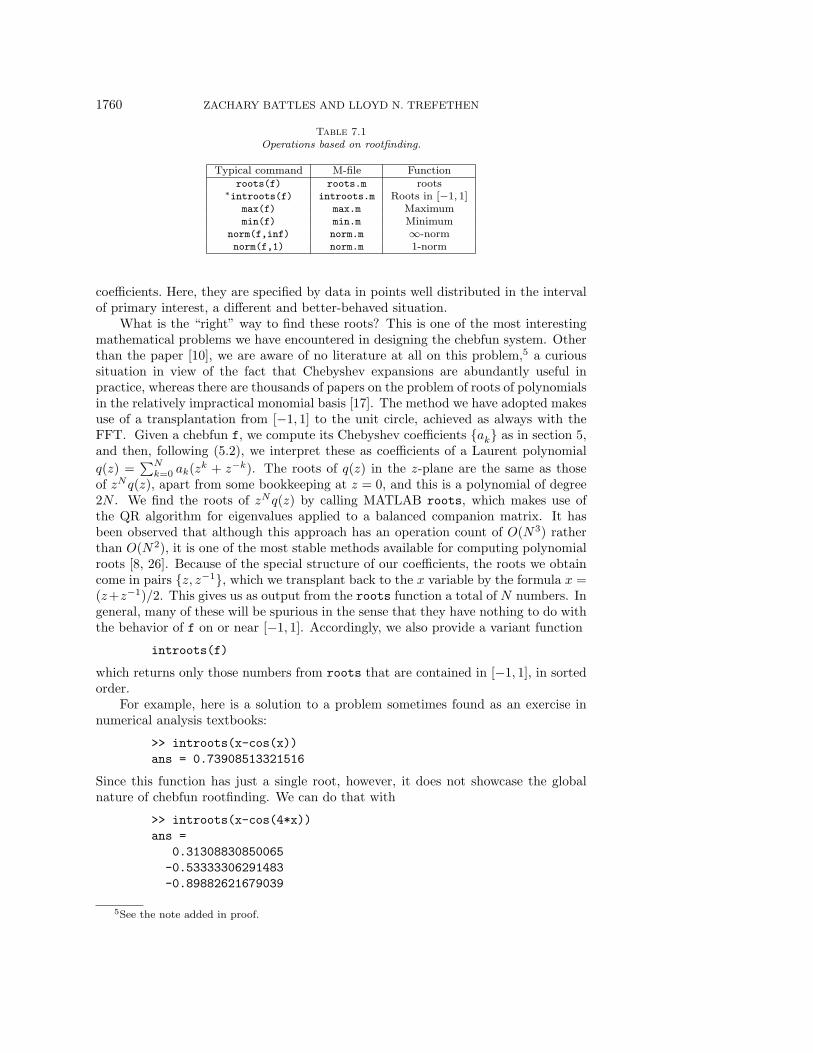
Table 7.1

Operations based on rootfinding.

Typical command M-file Functionroots(f) roots.m roots

∗introots(f) introots.m Roots in [−1, 1]max(f) max.m Maximummin(f) min.m Minimum

norm(f,inf) norm.m ∞-normnorm(f,1) norm.m 1-norm

coefficients. Here, they are specified by data in points well distributed in the intervalof primary interest, a different and better-behaved situation.

What is the “right” way to find these roots? This is one of the most interestingmathematical problems we have encountered in designing the chebfun system. Otherthan the paper [10], we are aware of no literature at all on this problem,5 a curioussituation in view of the fact that Chebyshev expansions are abundantly useful inpractice, whereas there are thousands of papers on the problem of roots of polynomialsin the relatively impractical monomial basis [17]. The method we have adopted makesuse of a transplantation from [−1, 1] to the unit circle, achieved as always with theFFT. Given a chebfun f, we compute its Chebyshev coefficients {ak} as in section 5,and then, following (5.2), we interpret these as coefficients of a Laurent polynomial

q(z) =∑N

k=0 ak(zk + z−k). The roots of q(z) in the z-plane are the same as those

of zNq(z), apart from some bookkeeping at z = 0, and this is a polynomial of degree2N . We find the roots of zNq(z) by calling MATLAB roots, which makes use ofthe QR algorithm for eigenvalues applied to a balanced companion matrix. It hasbeen observed that although this approach has an operation count of O(N3) ratherthan O(N2), it is one of the most stable methods available for computing polynomialroots [8, 26]. Because of the special structure of our coefficients, the roots we obtaincome in pairs {z, z−1}, which we transplant back to the x variable by the formula x =(z+z−1)/2. This gives us as output from the roots function a total of N numbers. Ingeneral, many of these will be spurious in the sense that they have nothing to do withthe behavior of f on or near [−1, 1]. Accordingly, we also provide a variant function

introots(f)

which returns only those numbers from roots that are contained in [−1, 1], in sortedorder.

For example, here is a solution to a problem sometimes found as an exercise innumerical analysis textbooks:

>> introots(x-cos(x))

ans = 0.73908513321516

Since this function has just a single root, however, it does not showcase the globalnature of chebfun rootfinding. We can do that with

>> introots(x-cos(4*x))

ans =

0.31308830850065

-0.53333306291483

-0.89882621679039

5See the note added in proof.


And here are the zeros in [0, 20] of the Bessel function J0(x):

>> f = chebfun(’besselj(0,10*(1+x))’);

>> 10*(1+introots(f))

ans =

2.40482555769577

5.52007811028631

8.65372791291101

11.79153443901428

14.93091770848778

18.07106396791093

These numbers are correct in every digit, except that the fifth one should end with79 instead of 78 and the sixth should end with 92 instead of 93.

With the ability to find roots in [−1, 1], we can now perform some other moreimportant operations. For example, if f is a chebfun, what is max(f)? The answershould be the global maximum on [−1, 1], and to compute this, we compute thederivative with diff, find its roots, and then check the value of f at these points andat ±1. The functions min(f) and norm(f,inf) are easy variants of this idea. Thus,for example,

>> f = x-x.^2;

>> min(f)

ans = -2

>> max(f)

ans = 0.25000000000000

>> [y,x] = max(f)

y = 0.25000000000000

x = 0.50000000000000

>> norm(f,inf)

ans = 2

The computation of a 1-norm by norm(f,1) is carried out by similar methods.The definition is

‖f‖1 =

∫ 1

−1

|f(x)|dx,

and since f may pass through 0, the integrand may have singularities in the form ofpoints of discontinuity of the derivative. To evaluate the integral we use introots

to find any roots of f in [−1, 1], divide into subintervals accordingly, and integrate.Thus norm(f,1) reduces to introots(f) and cumsum(f). For example, with f as inthe example above, we find

>> norm(f,1)

ans = 1

One can combine our functions rather nicely into a little program for computing thetotal variation of a function on [−1, 1]:

function tv = tv(f)

tv = norm(diff(f),1);


With tv defined in this fashion we find, for example,

>> tv(x)

ans = 2

>> tv(sin(5*pi*x))

ans = 20.00000000000005

The O(N3) operation count of our roots, min, and max computations is out ofline with the O(N logN) figure for most other chebfun calculations, and it makes theperformance unsatisfactory for N 100. There is not much literature on rootfind-ing for polynomials of high degrees, though an algorithm of Fox and Lindsey hasbeen applied to polynomials of degrees in the hundreds of thousands [24]. We areinvestigating the possible use of this or other rootfinding algorithms in the chebfunsystem.

8. Applications in numerical analysis. Having described a major part of thechebfun system, we can now consider more applications. To begin with, let us deter-mine some numbers of the kind that students learn how to compute in an introductorynumerical analysis course. For illustration we will take the function

f(x) = tan(x + 14 ) + cos(10x2 + ee

x

).(8.1)

The chebfun for this function (which turns out to have grid number N = 77) isconstructed in less than 0.1 sec. by

s = ’tan(x+1/4) + cos(10*x.^2+exp(exp(x)))’;

f = chebfun(s);

and the result of plot(f) is shown in Figure 8.1.One topic in a numerical analysis course is quadrature. A standard approach

using the built-in adaptive MATLAB code gives

>> quad(s,-1,1,1e-14)

ans = 0.29547767624377

in about 7 secs. on our workstation; MATLAB’s alternative code quadl reduces thisfigure to 1.6 secs. In the chebfun system, the adaptation has already taken place inconstructing the chebfun, and it takes just 0.02 secs. more to compute

>> sum(f)

ans = 0.29547767624377

Another basic topic is minimization. In standard MATLAB we find, for example,

>> opts = optimset(’tolx’,1e-14);

>> [x0,f0] = fminbnd(s,-1,1,opts)

x0 = -0.36185484293847

f0 = -1.09717538514564

From the figure it is evident that this result is a local minimum rather than the globalone. We can get the latter by refining the search interval:

>> [x0,f0] = fminbnd(s,-1,-.5,opts)

x0 = -0.89503073635821

f0 = -1.74828014625170

These calculations take around 0.05 secs. In the chebfun system the min function


−1 −0.5 0 0.5 1−2

0

2

4

Fig. 8.1. A function to illustrate quadrature, minimization, and rootfinding.

gives the global minimum directly:

>> [f0,x0] = min(f)

f0 = -1.74828014625170

x0 = -0.89503073653153

The timing is somewhat worse, 0.25 secs., because of the O(N3) rootfinding operation.Turning to rootfinding itself, in standard MATLAB we have

>> fzero(s,0)

ans = 0.24078098023501

and again it is clear from Figure 8.1 that this result is only local, since this functionhas three zeros in [−1, 1]. In the chebfun system we get them all at once:

>> introots(f)

ans =

0.24078098023501

-0.57439914100933

-0.75298521313936

We shall now consider two applications from the field of ordinary differentialequations (ODEs). The first is in the area known as waveform relaxation. Supposewe are given the nonlinear, variable coefficient ODE

u′ = e−2.75xu, −1 < x < 1, u(−1) = 0;(8.2)

we have picked the constant −2.75 to make the solution interesting. The problem canbe rewritten in integral form as

u(x) =

∫ x

−1

e−2.75suds,(8.3)

which suggests that we might try to solve (8.3) by Picard iteration, i.e., successivesubstitution. The following code carries out this process with chebfuns:

x = chebfun(’x’);

uold = chebfun(’0’);

du = 1

while du > 1e-13

u = cumsum(exp(-2.75*x.*uold));

du = norm(u-uold);

uold = u;

end

u(1)


−1 −0.5 0 0.5 10

2

4

6

Fig. 8.2. Solution of the ODE (8.2) by waveform relaxation.

−1 −0.5 0 0.5 1−3

−2

−1

0

1

Fig. 8.3. Solution of the boundary-value problem (8.4) using cumsum.

It takes around 7 secs. for the solution to be found, with u(1) = 5.07818302388064.The resulting chebfun, with N = 181, is plotted in Figure 8.2. For comparison, hereis a solution using standard ODE software:

opts = odeset(’abstol’,1e-14,’reltol’,1e-14);

[x,u] = ode45(@f,[-1,1],0,opts);

u(end)

function f = f(x,u)

f = exp(-2.75*x*u);

This code prints the number 5.07818302388075 in about 2 secs., and we do not claimthat the chebfun approach is in any way superior, merely that it is interesting. (We arein the process of considering extensions of our system to tackle ODEs more directly.)

A variation on this theme of waveform relaxation would be to use chebfuns iter-atively to find solutions to functional differential equations. We have used this ideasuccessfully for simple problems, such as finding a function f(x) on [−1, 1] such thatf(f(x)) = tanh(x), and are considering possible extensions to more challenging prob-lems such as the approximation of Feigenbaum’s constant or Daubechies wavelets.

Our next example, also from the field of ODEs, concerns the linear boundary-value problem

u′′ = e4x, −1 < x < 1, u(−1) = u(1) = 0.(8.4)

This problem is solved by a Chebyshev spectral method in Program 13 of [27]; theexact solution is u(x) = [e4x −x sinh(4)− cosh(4)]/16. We can solve it in the chebfunsystem with the sequence

f = exp(4*x);

u = cumsum(cumsum(f));

u = u - u(1).*(1+x)/2;

and Figure 8.3 shows the result, which is accurate to 14 digits.


9. Chebfun quasi matrices. We are finally ready to move from vectors to ma-trices (Table 9.1). Specifically, in this section we consider “matrices” that consist of adiscrete set of columns, each of which is a chebfun of the kind we have been discussing.Thus our matrices are continuous in the row dimension, discrete in the column dimen-sion. The idea of such objects is surely an old one, and they are mentioned explicitlyby de Boor [6] (“column maps”), Trefethen and Bau [28, p. 52] (“matrices with con-tinuous columns”), and Stewart [25, p. 33] (“quasi matrices”). To be definite we shalluse the latter term.

We can explain the idea with an example built on x = chebfun(’x’) as usual:

>> A = [1 x x.^2 x.^3 x.^4]

A = column chebfun

1.0000 1.0000 1.0000 1.0000 1.0000

1.0000 0.7071 0.5000 0.3536 0.2500

1.0000 0 0 0 0

1.0000 -0.7071 0.5000 -0.3536 0.2500

1.0000 -1.0000 1.0000 -1.0000 1.0000

>> size(A)

ans =

-4 5

We see that A is a matrix of five columns, each of which is a chebfun. In principle,each might have a different grid value N , in which case the Chebyshev point datadefining A could be stored in a MATLAB cell array, but our implementation insteadforces all columns to share the same maximal value of N and stores the data in anordinary matrix. We can evaluate A at various points by commands like these:

>> A(3,5)

ans = 81.0000

>> A(0.5,:)

ans =

1.0000 0.5000 0.2500 0.1250 0.0625

>> A(:,3)


1.0000

0.5000

0

0.5000

1.0000

Note that in each case the first argument is a function argument, and the second isan index.

If c is a column vector of the appropriate dimension (namely, size(A,2)), theproduct A*c should be a chebfun equal to the linear combination of the columns of Awith the given coefficients. Thus the sequence

>> c = [1 0 -1/2 0 1/24]’;

>> f = A*c;

>> norm(f-cos(x),inf)

ans = 0.0014

reveals that the maximum deviation of cosx on [−1, 1] from its fourth-order Taylor


Table 9.1

Operations involving quasi matrices.

Typical command M-file Function

A = [f g h] horzcat.m Construction of quasi matrix

A([.5 .6],[2 3]) subsref.m Evaluate at specified points

A*x mtimes.m Quasi matrix times vector

[Q,R] = qr(A,0) qr.m QR factorization

[U,S,V] = svd(A,0) svd.m Singular value decomposition

cond(A) cond.m Condition number

rank(A) rank.m Rank

null(A) null.m Basis of nullspace

pinv(A) pinv.m Pseudoinverse

norm(A) norm.m Norm

A\b mldivide.m Least-squares solution

A’*B mtimes.m Inner product of quasi matrices

series approximation is about 0.0014. The figure becomes twenty times smaller forthe degree 4 Chebyshev interpolant, whose coefficients are only very slightly different:

>> c = poly(chebfun(’cos(x)’,4))

c =

0.0396 0 -0.4993 0 1.0000

>> f = A*c(end:-1:1)’;

>> norm(f-cos(x),inf)

ans = 6.4809e-05

Many familiar matrix operations make sense for quasi matrices. For example, ifA is a quasi matrix with n chebfun columns, then in the (reduced) QR decompositionA = QR, Q will be another quasi matrix of the same dimension whose columns areorthonormal, and R will be an n × n upper-triangular matrix. The chebfun systemperforms the computation by a modified Gram–Schmidt method:

[Q,R] = qr(A,0)

Q = column chebfun

0.7071 1.2247 1.5811 1.8708 2.1213

0.7071 0.8660 0.3953 -0.3307 -0.8618

0.7071 0 -0.7906 -0.0000 0.7955

0.7071 -0.8660 0.3953 0.3307 -0.8618

0.7071 -1.2247 1.5811 -1.8708 2.1213

R =

1.4142 0 0.4714 0 0.2828

0 0.8165 0 0.4899 -0.0000

0 0 0.4216 -0.0000 0.3614

0 0 0 0.2138 -0.0000

0 0 0 0 0.1077

Similarly, the (reduced) SVD of A should be a factorization A = USV T , where Uhas the same type as A, S is n × n and diagonal with nonincreasing nonnegativediagonal entries, and V is n × n and orthogonal. We compute this by computingfirst the reduced QR decomposition A = QR as above and then the ordinary SVDR = U1SV

T ; we then have A = USV T with U = QU1:


[U,S,V] = svd(A,0)

U = column chebfun

0.9633 -1.4388 1.7244 -1.7117 -1.8969

0.7440 -0.8205 0.1705 0.4315 0.9035

0.5960 0.0000 -0.7747 0.0000 -0.8958

0.7440 0.8205 0.1705 -0.4315 0.9035

0.9633 1.4388 1.7244 1.7117 -1.8969

S =

1.5321 0 0 0 0

0 0.9588 0 0 0

0 0 0.5181 0 0

0 0 0 0.1821 0

0 0 0 0 0.0809

V =

0.9130 0.0000 -0.4014 -0.0000 -0.0725

-0.0000 -0.8456 -0.0000 0.5339 0.0000

0.3446 -0.0000 0.6640 -0.0000 0.6636

-0.0000 -0.5339 -0.0000 -0.8456 -0.0000

0.2182 -0.0000 0.6308 0.0000 -0.7446

The function svd by itself gives just the singular values, i.e., the diagonal entries of S,which can be interpreted as the semiaxis lengths of the hyperellipsoid that is the imageof the unit ball in n-space under A. The function cond gives the ratio of the maximumand minimum singular values, and rank counts the number of singular values abovea prescribed tolerance, which defaults to a number on the order of machine precision.Thus after the above calculations we have

>> cond(A)

ans = 18.9286

>> cond(Q)

ans = 1.0000

>> rank(A)

ans = 5

>> rank([1 x.^2 x.^2])

ans = 2

>> rank([sin(x) sin(2*x) sin(3*x) sin(4*x)])

ans = 4

>> rank([sin(2*x) sin(x).*cos(x)])

ans = 1

A moment ago we computed the QR factorization of the quasi matrix withcolumns 1, x, x2, x3, x4. The resulting Q is a quasi matrix whose columns are orthog-onal polynomials, each normalized to have 2-norm equal to 1. Thus the columns ofQ are the Legendre polynomials, except that the latter are conventionally normalizedto take the value 1 at x = 1. We can achieve that normalization like this:

>> for i = 1:5;

P(:,i) = Q(:,i)/Q(1,i);

end

plot(P)


−1 −0.5 0 0.5 1

−1

0

1

Fig. 9.1. The first five Legendre polynomials, computed by QR decomposition of the quasimatrix whose columns are chebfuns for 1, x, x2, x3, x4.

which produces the familiar picture of Figure 9.1. For example, here are the coeffi-cients of P4(x):

>> poly(P(:,5))

ans =

4.3750 -0.0000 -3.7500 0.0000 0.3750

From the QR factorization comes a ready ability to solve least-squares problems,and this is implemented in an overloaded \ operator:

>> c = A\cos(x)

c =

1.0000

-0.0000

-0.4994

0.0000

0.0398

>> norm(A*c-cos(x),inf)

ans = 9.2561e-05

Note that this is comparable to the result found earlier by interpolation in Chebyshevpoints.

Stewart has a half-serious remark in a footnote on p. 34 of his Afternotes Goes toGrad School [25]:

If you introduce a formal mathematical object, people are likely to start

writing papers about it. Like “On the generalized inverse of quasi-matrices.”

Ugh!

Well, Pete, here we are, sooner than you could have imagined:

>> pinv(A)

ans = row chebfun

0.9375 -0.4980 1.7578 -0.4980 0.9375

-3.7500 1.9887 -0.0000 -1.9887 3.7500

-13.1250 7.7930 -8.2031 7.7930 -13.1250

8.7500 -1.5468 0.0000 1.5468 -8.7500

19.6875 -7.9980 7.3828 -7.9980 19.6875

The implementation is [U,S,V] = svd(A,0), pinv = V*inv(S)*U’.

10. Conclusion. The chebfun system is under development. One of our goalsis to find ways to make it more effective at solving problems by spectral collocation


methods such as those embodied in the MATLAB programs of [27]. Another, alreadypartly achieved, is to extend the system to the case of “matrices” that are continuousin both the column and row dimensions rather than just the latter. Such objects canbe regarded as bivariate functions on [−1, 1]×[−1, 1] or as integral operators. We havealready implemented a good deal of this functionality and hinted at the possibility ofcontinuity in the column dimension in the discussions of f’*g and pinv, but we willnot give details here as they have not yet settled down.

Computation in the chebfun system has a hybrid flavor: the feel is symbolic, butthe implementation is numerical. Having become used to this style of programming,we find it powerful and appealing. Of course, true symbolic computation wouldgenerally be better for those problems where it is applicable, but these are a minority.6

The class of problems whose solutions are merely smooth, as we have targeted here,is much wider.

Many topics of numerical analysis can be illustrated in the chebfun system, as wellas some fundamental ideas of approximation theory, functional analysis, and object-oriented programming; one can imagine many classrooms to which this system mightbe able to contribute. MATLAB itself was originally introduced as an educationaltool, but eventually, it proved to be much more than that. Perhaps the chebfunsystem too will mature in interesting ways.

Note added in proof. Since this paper was accepted for publication we havebecome aware of a paper by Boyd that presents some of the same ideas [2]. Boyd isnot concerned with general operations on functions, nor with overloading MATLABcommands, but with the specific subject of finding zeros of a function on an interval.The algorithm he proposes is the same as ours in two crucial respects: he approximatesthe function by a Chebyshev series of adjustable degree, and he finds the roots ofthis approximation by a change of variables that transplants the unit interval to theunit circle. Boyd then introduces a third powerful idea: recursive subdivision of therootfinding interval to reduce the cubic operation count that is otherwise entailedin rootfinding. Following his lead, we have subsequently introduced recursion in thechebfun rootfinding operations too and thereby reduced the computing time for suchoperations, for large degrees, by an order of magnitude.

Acknowledgments. We are grateful to Jean-Paul Berrut, Folkmar Bornemann,Kevin Burrage, Carl de Boor, David Handscomb, Des Higham, Nick Higham, CleveMoler, Pete Stewart, Peter Vertesi, and Andy Wathen for commenting on drafts ofthis article, suggesting applications, and pointing us to relevant literature.

REFERENCES

[1] J.-P. Berrut and L. N. Trefethen, Barycentric Lagrange interpolation, SIAM Rev., 46 (3)(2004), to appear.

[2] J. A. Boyd, Computing zeros on a real interval through Chebyshev expansion and polynomialrootfinding, SIAM J. Numer. Anal., 40 (2002), pp. 1666–1682.

[3] L. Brutman, Lebesgue functions for polynomial interpolation—a survey, Ann. Numer. Math.,4 (1997), pp. 111–128.

[4] C. W. Clenshaw and A. R. Curtis, A method for numerical integration on an automaticcomputer, Numer. Math., 2 (1960), pp. 197–205.

[5] P. J. Davis and P. Rabinowitz, Methods of Numerical Integration, 2nd ed., Academic Press,New York, 1984.

6See the appendix “The definition of numerical analysis” in [28].


[6] C. de Boor, An alternative approach to (the teaching of) rank, basis, and dimension, LinearAlgebra Appl., 146 (1991), pp. 221–229.

[7] D. Gaier, Lectures on Complex Approximation, Birkhauser, Boston, 1987.[8] S. Goedecker, Remark on algorithms to find roots of polynomials, SIAM J. Sci. Comput., 15

(1994), pp. 1059–1063.[9] D. Gottlieb, M. Y. Hussaini, and S. A. Orszag, Theory and applications of spectral methods,

in Spectral Methods for Partial Differential Equations, R. G. Voigt, D. Gottlieb, and M. Y.Hussaini, eds., SIAM, Philadelphia, 1984, pp. 1–54.

[10] J. A. Grant and A. Ghiatis, Determination of the zeros of a linear combination of Chebyshevpolynomials, IMA J. Numer. Anal., 3 (1983), pp. 193–206.

[11] N. J. Higham, The numerical stability of barycentric Lagrange interpolation, IMA J. Numer.Anal., to appear.

[12] T. W. Korner, Fourier Analysis, Cambridge University Press, Cambridge, UK, 1988.[13] A. R. Krommer and C. W. Ueberhuber, Computational Integration, SIAM, Philadelphia,

1998.[14] G. G. Lorentz, Approximation of Functions, 2nd ed., Chelsea, New York, 1986.[15] J. C. Mason and D. C. Handscomb, Chebyshev Polynomials, Chapman & Hall/CRC, Boca

Raton, FL, 2003.[16] G. Mastroianni and J. Szabados, Jackson order of approximation by Lagrange interpolation.

II, Acta Math. Hungar., 69 (1995), pp. 73–82.[17] J. M. McNamee, A bibliography on roots of polynomials, J. Comput. Appl. Math., 47 (1993),

pp. 391–392; also available online from www.elsevier.com/homepage/sac/cam/mcnamee/.[18] G. Meinardus, Approximation of Functions: Theory and Numerical Methods, Springer-Verlag,

Berlin, 1967.[19] C. B. Moler, ROOTS—Of polynomials, that is, MathWorks Newsletter, 5 (1991), pp. 8–9.[20] A. V. Oppenheim and R. W. Schafer, Discrete-Time Signal Processing, Prentice-Hall, En-

glewood Cliffs, NJ, 1989.[21] T. Ransford, Potential Theory in the Complex Plane, Cambridge University Press, Cam-

bridge, UK, 1995.[22] T. J. Rivlin, Chebyshev Polynomials: From Approximation Theory to Algebra and Number

Theory, Wiley, New York, 1990.[23] H. E. Salzer, Lagrangian interpolation at the Chebyshev points xn,ν = cos(νπ/n), ν = 0(1)n;

some unnoted advantages, Computer J., 15 (1972), pp. 156–159.[24] G. A. Sitton, C. S. Burrus, J. W. Fox, and S. Treitel, Factorization of very high degree

polynomials in signal processing, IEEE Signal Process. Mag., 20 (2003), pp. 27–42.[25] G. W. Stewart, Afternotes Goes to Graduate School: Lectures on Advanced Numerical Anal-

ysis, SIAM, Philadelphia, 1998.[26] K.-C. Toh and L. N. Trefethen, Pseudozeros of polynomials and pseudospectra of companion

matrices, Numer. Math., 68 (1994), pp. 403–425.[27] L. N. Trefethen, Spectral Methods in MATLAB, SIAM, Philadelphia, 2000.[28] L. N. Trefethen and David Bau III, Numerical Linear Algebra, SIAM, Philadelphia, 1997.[29] L. N. Trefethen and J. A. C. Weideman, Two results on polynomial interpolation in equally

spaced points, J. Approx. Theory, 65 (1991), pp. 247–260.[30] J. L. Walsh, Interpolation and Approximation by Rational Functions in the Complex Domain,

5th ed., AMS, Providence, RI, 1969.[31] J. H. Wilkinson, The perfidious polynomial, in Studies in Numerical Analysis, G. H. Golub,

ed., Math. Assoc. Amer., Washington, D.C., 1984, pp. 1–28.

an extension of matlab to continuous functions and … · an extension of matlab to continuous...

Documents