an extensional mode resonator for vibration …
TRANSCRIPT

AN EXTENSIONAL MODE RESONATOR
FOR VIBRATION HARVESTING
By
JOHN Mc KAY YOUNGSMAN
A dissertation submitted in partial fulfillment of the requirements for the degree of
DOCTOR OF PHILOSOPHY
WASHINGTON STATE UNIVERSITY College of Engineering and Architecture
MAY 2009

ii
To the Faculty of Washington State University:
The members of the Committee appointed to examine the dissertation of John
Mc Kay Youngsman find it satisfactory and recommend that it be accepted.
___________________________________ David F. Bahr, Ph.D., Chair ___________________________________ Michael J. Anderson, Ph.D. ___________________________________ David P. Field, Ph.D. ___________________________________ M. Grant Norton, Ph.D.

iii
ACKNOWLEDGEMENT
A dissertation is never accomplished by an individual. There is always a tremendous
supporting cast. I have been very fortunate to be surrounded by incredibly supportive people. I would
like to express my gratitude and appreciation to the following people for their efforts in helping me
achieve the production of this work:
Professor David Bahr, my advisor, for accepting me into his group, providing sage advice, and
giving me the opportunity to work on such an interesting project.
Professor Michael Anderson, committeeman, for the hours of assistance and direction in this
work.
Professors David Field, and Grant Norton, my committee, for their time and interest in my
work.
Dr. Dylan Morris for his inspiration and creation of the first prototype XMR.
Tim Luedeman, summer intern, for his outstanding assistance and dedicated work.
Bob Ames, my friend and golfing partner, who provided sanity checks through the last half of
this work.
Finally, to Cheryl, Abby, and Max for their love and patience to endure my absence for much
longer than originally planned.
Financial support was provided through the US Navy under a subcontract to an SBIR project
with TPL Incorporated; contract number N68335-08-C-0098.

iv
AN EXTENSIONAL MODE RESONATOR
FOR VIBRATION HARVESTING
ABSTRACT
By John Mc Kay Youngsman, Ph.D.
Washington State University
May 2009
Chair: David F. Bahr
In an effort to identify techniques for harvesting energy from ambient vibrations, a prototype device
that utilizes stretching piezoelectric film to support a proof mass, with an adjustable support that
allows the resonant frequency of the device to be easily altered has been developed. This extensional
mode resonator (XMR) device is described by a model developed in this work that predicts the power
that is harvested as a function of the frequency and amplitude of the external vibration, the elastic and
piezoelectric materials properties, and the device geometry. The model provides design guidelines for
the effects of device geometry and applied tension through an adjustable support that suggest a strong
dependence on mechanical damping and a weak dependence on frequency, as opposed to a bending
cantilever device. The model predictions are compared to experimental measures from multiple
configurations of the prototype device for frequencies between 60 Hz and 180 Hz, and at accelerations
between 0.1 m/s2 and 25 m/s2. Up to 22 mW is generated from a device with a mass of ~82 g at

v
25 m/s2 acceleration, and over the range of frequencies tested the power harvested at 4 m/s2 is between
3 mW and 4 mW. The developed models are used as design tools for various configurations that are
capable of over 100 mW at less than 3 m/s2 in one case to another that can generate more than 10 mW
at 1 m/s2. Prototype configurations have been successfully tested as high as 80 m/s2 with power
generated on the order of 40 mW.

vi
TABLE OF CONTENTS
ACKNOWLEDGEMENT ...................................................................................................................... iii
ABSTRACT ........................................................................................................................................... iv
TABLE OF CONTENTS ....................................................................................................................... vi
LIST OF TABLES .................................................................................................................................. x
LIST OF FIGURES ................................................................................................................................ xi
CHAPTER ONE ..................................................................................................................................... 1
1 INTRODUCTION ............................................................................................................................ 1
1.1 Power Requirements .................................................................................................................. 2
1.2 Principle of Piezoelectricity ...................................................................................................... 3
1.3 Polymer Piezoelectric Materials ................................................................................................ 6
1.4 Conformation Effects ................................................................................................................ 7
1.5 Poling Techniques ..................................................................................................................... 9
1.6 Review of Cantilever Type Devices ........................................................................................ 10
1.7 Stretching Mode ...................................................................................................................... 11
CHAPTER TWO ................................................................................................................................... 13
2 PVDF POLING AND TESTING TECHNIQUES ......................................................................... 13
2.1 Introduction ............................................................................................................................. 13
2.2 Poling ...................................................................................................................................... 13
2.3 Evaluating Phase ..................................................................................................................... 16

vii
2.4 Measuring Compliance s11E ..................................................................................................... 21
2.5 Measuring Piezoelectric Coefficient, d31 ................................................................................. 27
2.6 Amplitude Measurements ........................................................................................................ 31
2.7 Damping .................................................................................................................................. 33
CHAPTER THREE ............................................................................................................................... 39
3 XMR BASICS ................................................................................................................................ 39
3.1 Introduction ............................................................................................................................. 39
3.2 The Extensional Mode Resonator ........................................................................................... 41
3.3 Prototype Device Fabrication and Experimental Measures .................................................... 43
3.4 Frequency Tunability .............................................................................................................. 45
3.5 Power Results of the XMR ...................................................................................................... 49
3.6 Conclusions ............................................................................................................................. 51
CHAPTER FOUR ................................................................................................................................. 52
4 MODEL DEVELOPMENT OF THE RXMR ................................................................................ 52
4.1 Introduction ............................................................................................................................. 52
4.2 Dynamic Model ....................................................................................................................... 55
4.3 Electric Circuit Analysis and Energy Harvesting Capability .................................................. 60
4.4 Prototype Device ..................................................................................................................... 63
4.5 Electrical Impedance ............................................................................................................... 63
4.6 Mechanical Vibration and Power Output ................................................................................ 64
4.7 Results ..................................................................................................................................... 66

viii
4.8 Mechanical Vibration and Power Output ................................................................................ 68
4.9 Uncertainty Discussion ............................................................................................................ 73
4.10 Conclusions ........................................................................................................................... 74
CHAPTER FIVE ................................................................................................................................... 75
5 EXCESS FILM MODEL DEVELOPMENT ................................................................................. 75
5.1 Introduction ............................................................................................................................. 75
5.2 Geometric Effects .................................................................................................................... 75
5.3 Development of Power Equations ........................................................................................... 79
5.4 Experimental Results of Excess Model ................................................................................... 85
CHAPTER SIX ..................................................................................................................................... 92
6 APPLICATIONS OF THE DEVELOPED MODELS TO DESIGN ............................................. 92
6.1 Introduction ............................................................................................................................. 92
6.2 Matchbox Device .................................................................................................................... 93
6.3 CD Jewel Case Device ............................................................................................................ 97
6.4 ½ Pint Carton Device ............................................................................................................ 102
6.5 Conclusions ........................................................................................................................... 106
CHAPTER SEVEN ............................................................................................................................. 108
7 CONCLUSIONS .......................................................................................................................... 108
REFERENCES .................................................................................................................................... 113
APPENDIX ......................................................................................................................................... 117
A1 Materials Properties Information ........................................................................................... 118

ix
A2 RXMR Excess Model Development Equations from Mathematica ...................................... 122
A3 Composite Material Thickness Derivation ............................................................................ 151
A4 Uncertainty Analysis ............................................................................................................. 155
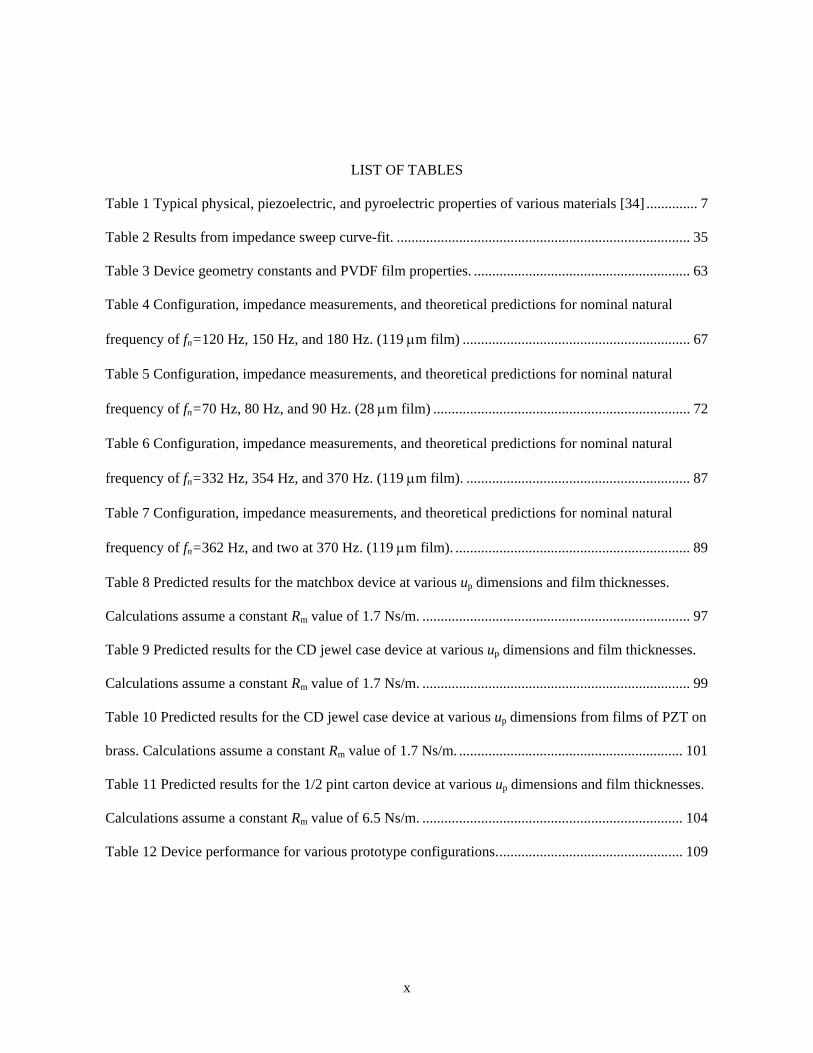
x
LIST OF TABLES
Table 1 Typical physical, piezoelectric, and pyroelectric properties of various materials [34] .............. 7
Table 2 Results from impedance sweep curve-fit. ................................................................................ 35
Table 3 Device geometry constants and PVDF film properties. ........................................................... 63
Table 4 Configuration, impedance measurements, and theoretical predictions for nominal natural
frequency of fn=120 Hz, 150 Hz, and 180 Hz. (119 µm film) .............................................................. 67
Table 5 Configuration, impedance measurements, and theoretical predictions for nominal natural
frequency of fn=70 Hz, 80 Hz, and 90 Hz. (28 µm film) ...................................................................... 72
Table 6 Configuration, impedance measurements, and theoretical predictions for nominal natural
frequency of fn=332 Hz, 354 Hz, and 370 Hz. (119 µm film). ............................................................. 87
Table 7 Configuration, impedance measurements, and theoretical predictions for nominal natural
frequency of fn=362 Hz, and two at 370 Hz. (119 µm film). ................................................................ 89
Table 8 Predicted results for the matchbox device at various up dimensions and film thicknesses.
Calculations assume a constant Rm value of 1.7 Ns/m. ......................................................................... 97
Table 9 Predicted results for the CD jewel case device at various up dimensions and film thicknesses.
Calculations assume a constant Rm value of 1.7 Ns/m. ......................................................................... 99
Table 10 Predicted results for the CD jewel case device at various up dimensions from films of PZT on
brass. Calculations assume a constant Rm value of 1.7 Ns/m. ............................................................. 101
Table 11 Predicted results for the 1/2 pint carton device at various up dimensions and film thicknesses.
Calculations assume a constant Rm value of 6.5 Ns/m. ....................................................................... 104
Table 12 Device performance for various prototype configurations. .................................................. 109

xi
LIST OF FIGURES
Figure 1 Examples of noncentrosymmetric crystal structures [28] ......................................................... 3
Figure 2 Schematic detailing the 31 and 33 mode of piezoelectric materials [29]. ................................. 4
Figure 3 Schematic detailing the composite structure of piezoelectric fibers embedded in an epoxy
matrix with interdigitated electrodes configured to take advantage of the higher d33 coefficient of
piezoelectricity [30]. ................................................................................................................................ 5
Figure 4 SEM image of a MEMS curved cantilever with an interdigitated electrode design to utilize
the d33 coefficient [31]. ............................................................................................................................ 6
Figure 5 Stress strain curve for PVDF [33]. ............................................................................................ 7
Figure 6 Schematic depiction of the two most common crystalline chain conformations in PVDF: (a)
tg+tg- and (b) all-trans. The arrows indicate projections of the -CF2 dipole directions on planes defined
by the carbon backbone. The tg+tg- conformation has components of the dipole moment both parallel
and perpendicular to the chain axis, while the all-trans conformation has all dipoles essentially normal
to the molecular axis [34]. ....................................................................................................................... 8
Figure 7 Schematic showing the random distribution of amorphous material and small crystallites in
cast PVDF (top). Application of strain (middle) orients the crystallites along a single axis. Poling
(bottom) aligns the dipoles of the crystallites [32]. ................................................................................. 9
Figure 8 RXMR device. A proof mass is suspended by PVDF films which stretch rather than bend
during vibratory motion. Adjustment screws change tension. .............................................................. 12
Figure 9 Cross section view of conical XMR. ...................................................................................... 12
Figure 10 Poling apparatus. Top left: hot plate with sample in dielectric bath. Top right: sample on
conductive base and copper contact pad. Bottom: Bertran power supply and ammeter. ...................... 14

xii
Figure 11 Current vs. time for the poling process of sample AM75 13B. Each step increase in current
at time < 20 minutes represents a 50 V step in the applied field. .......................................................... 15
Figure 12 FTIR spectra from 28 µm Measurement Specialties film. The peak at ~840 cm-1 indicates
presence of β-phase. Peaks at ~615 and ~763 cm-1 indicate α-phase. .................................................. 17
Figure 13 FTIR spectrum from TPL, Inc. cast film. The peak at ~840 cm-1 indicate β-phase while the
broad peak below 700 cm-1 hides most information regarding α-phase. .............................................. 18
Figure 14 FTIR spectrum from TPL, Inc. cast film sample AM75-21A. .............................................. 19
Figure 15 FTIR spectra for stretched (red) vs. unstretched (blue) PVDF-HFP 10% sample from TPL
(AM75-49A). ......................................................................................................................................... 20
Figure 16 FTIR spectra for stretched (red) vs. unstretched (blue) PVDF-HFP 10% with 20 vol% PZT
sample from TPL (AM75-13B). ............................................................................................................ 20
Figure 17 Stress vs. strain results from a DMA test on samples of 9 µm biaxial stretched PVDF film.
............................................................................................................................................................... 22
Figure 18 Linear region of stress vs. strain results from a DMA test on samples of 9 µm biaxial
stretched PVDF film showing curve fit of samples. .............................................................................. 22
Figure 19 Zoomed in region of stress vs. strain results from a DMA test on samples of 9 µm biaxial
stretched PVDF film showing a curve fit of the sample data that corresponds to the materials modulus.
............................................................................................................................................................... 23
Figure 20 Schematic of bulge test apparatus used for measuring film modulus. .................................. 24
Figure 21 Pressure vs. deflection data with curve fit of Measurement Specialties 28 µm film used to
calculate film modulus. ......................................................................................................................... 25
Figure 22 Schematic of the force-deflection experiment using the 4-point bend apparatus. ................ 26
Figure 23 Force-displacement measurement relationship of the RXMR used as a method to determine
compliance. (Data file 10140816 corrected load plot.) ......................................................................... 27
Figure 24 Schematic of d31 gravity test. ................................................................................................ 28

xiii
Figure 25 Schematic of d31 experiment using the bulge test apparatus. ................................................ 30
Figure 26 Drawing of the electrode generated by the shadow mask used in the RMM d31 bulge test. . 31
Figure 27 Typical plot showing the displacement vs. acceleration of the mass and base. The
displacements between the mass and base differ by more than an order of magnitude. ....................... 32
Figure 28 Plot showing the measured mass amplitude vs. base acceleration of the XMR at resonant
frequencies of 152 Hz and 178 Hz. ....................................................................................................... 33
Figure 29 Initial impedance sweep, vs.Z f , (left) and curvefit (right) of impedance data of the XMR
device nominally tuned to 180 Hz. ........................................................................................................ 34
Figure 30 Image of the XMR device with binder clips attached. .......................................................... 34
Figure 31 Impedance sweep, vs.Z f , (left) and curvefit (right) of impedance data of the XMR device
after the attachment of additional mass. ................................................................................................ 35
Figure 32 Mechanical damping Rm vs. up+uxs generated from data sets. Blue data are from 119 µm
films, red data are from 28 µm films, diamonds are from a regular model device, triangles are from an
xs-model device. .................................................................................................................................... 38
Figure 33 (a)Schematic of the displacement u of a rectangular string of non-deformed length 2l,
thickness h and width w (out of the plane of the figure) at the center by a force F. (b) Pre-tensioning
two extensional elements by a rigid link of length 2up. (c) Displacement of the link by an external
force F by an amount ∆u. ...................................................................................................................... 42
Figure 34 (a) Section view of the XMR (b) Photograph of an assembled XMR device ...................... 44
Figure 35 Cross-sectional schematic of the XMR device driven by base excitation. In this schematic,
the seismic mass has moved upwards relative to the base, causing the top piezoelectric membrane to
shorten and the bottom membrane to lengthen. Continued vibratory motion causes the membranes to
alternately lengthen and shorten [24]. ................................................................................................... 45

xiv
Figure 36 Frequency response functions from a frequency-tuning experiment in which each symbol
indicates the same adjustment position. Different experiments at each adjustment position have
different shading. The adjustment was varied between the three positions in a random sequence. This
demonstrates the reproducibility of the frequency tuning mechanism. ................................................. 46
Figure 37 Resonant frequency, determined by the frequency response function, as a function of
relative preloading displacement. The placement of the preloading screw at 212 Hz is an arbitrary
datum. The solid line is a least-squares linear fit, and the dashed lines indicate a 95 % confidence
interval [24]. .......................................................................................................................................... 47
Figure 38 Compressive beam technique (a) schematic of technique (b) device under test [19]. .......... 48
Figure 39 Magnetic assist by Challa et al (a) magnet configuration that increases the effective stiffness
of the beam (b) magnet configuration that decreases the effective stiffness of the beam. (c) Device
schematic showing positions of components [20]. ................................................................................ 48
Figure 40 Schematic of Hu et al method to load a bimorph cantilever [54]. ........................................ 49
Figure 41 Power vs. acceleration for the prototype XMR. .................................................................... 50
Figure 42 Power vs. acceleration of the prototype XMR at low acceleration amplitudes. ................... 51
Figure 43 Schematic for mechanical function of the XMR device. ...................................................... 54
Figure 44 Schematic for electrical function of the device. .................................................................... 55
Figure 45 A free-body diagram for the mass m. .................................................................................... 56
Figure 46 Equivalent circuit diagram for the device (Equations (4.13) and (4.20)). ............................ 61
Figure 47 Measurement of electrical impedance and curve fit for circuit parameters R, L, C, Co and k2.
............................................................................................................................................................... 64
Figure 48 Apparatus used to perform power output experiment from a controlled vibration source. .. 65
Figure 49 Transfer function vs. frequency of the XMR device. Peak indicates the resonant frequency
of the oscillator. ..................................................................................................................................... 66

xv
Figure 50 Comparison of predicted power output vs. acceleration for the XMR configured with
nominal natural frequencies of 120, 150, and 180 Hz. .......................................................................... 69
Figure 51 Power output vs. acceleration for the XMR across a broad range of frequencies. Device was
constructed with 119 µm films. ............................................................................................................. 70
Figure 52 Power output vs. acceleration for the XMR configured with nominal natural frequencies of
40, 48, and 59 Hz. Device was constructed with 9 µm films. ............................................................... 71
Figure 53 Comparison of predicted power output vs. acceleration for the XMR configured with
nominal natural frequencies of 70, 80, and 90 Hz. Device was constructed with 28 µm films. ........... 72
Figure 54 XS model geometric configuration (left) unstrained configuration, (middle) static strained
film due to up tension, (right) dynamic strained films due to base motion ∆u. ..................................... 76
Figure 55 Plot of power function vs. uxs. Acceleration normalized power variation with changes in
excess film length for a device configured with 119 µm film, 82.3 g mass, and dimensions of
Lo= 22 mm, w= 24 mm, and up= 3.59 mm. ........................................................................................... 81
Figure 56 Dimensionless term RCoωn vs. uxs. Variation of the RCoωn term with additions to the film
length. .................................................................................................................................................... 82
Figure 57 Resonant frequency response to changes in excess film length. ........................................... 82
Figure 58 Device stiffness vs. changes in excess film length. .............................................................. 83
Figure 59 Predicted frequency response of xs-model versus changes in uxs at several values of up. (red
(long dash): up=3 mm, green (short dash): up=4 mm, black (solid): up=5 mm) .................................... 84
Figure 60 Predicted frequency response of xs-model versus changes in up at several values of uxs. (red
(long dash): uxs=0, green (short dash): uxs=10 mm, black (solid): uxs=20 mm) .................................... 85
Figure 61 Measured power vs. acceleration data with theoretical predictions for an xs-model device. 88
Figure 62 Measured power vs. acceleration data with theoretical predictions for an xs-model device. 89
Figure 63 Power vs. acceleration plot of xs-model device from two separate data runs. The dimension
up is the same between the 354 Hz measurement and the 362 Hz measurement indicating potential

xvi
creep. Blue data set was taken approximately two weeks before the red set. Two different up settings
generated 378 Hz data in the latter set. ................................................................................................. 90
Figure 64 Power vs. acceleration plot of xs-model device (blue) contrasted with the regular model
(red). Mass and film thickness are the same. Film length is the significant variation between the two
results. ................................................................................................................................................... 91
Figure 65 Model of the matchbox size device. ...................................................................................... 93
Figure 66 Front view of the matchbox device showing device configuration and clearance. ............... 94
Figure 67 Partial section view of the matchbox device. ........................................................................ 95
Figure 68 Predicted power vs. acceleration for the matchbox device showing performance from a
device constructed with two sizes of PVDF film. Results of 31, 62 and 92 Hz are from 28 µm film, the
remaining are from 119 µm film. .......................................................................................................... 96
Figure 69 Model of the CD jewel case device. ..................................................................................... 98
Figure 70 Front view of the CD jewel case device showing device configuration and clearance. ....... 98
Figure 71 Predicted power vs. acceleration for the CD jewel case device showing performance from a
device constructed with two sizes of PVDF film. Results of 3.7, 5.6 and 7.4 Hz are from 28 µm film,
the remaining are from 119 µm film. .................................................................................................... 99
Figure 72 Predicted power vs. acceleration for the CD jewel case device showing performance from a
device constructed with PZT on brass foils. Results of 3.7 Hz (PVDF 28 µm film) and 8 Hz (PVDF
119 µm film) are shown for comparison. ............................................................................................ 101
Figure 73 Model of the 1/2 pint carton device designed with a copper mass and PVDF films. ......... 102
Figure 74 Front view of the 1/2 pint carton device showing relationship between components. ....... 103
Figure 75 Section view of the 1/2 pint carton device showing additional relations between
components. ......................................................................................................................................... 103

xvii
Figure 76 Predicted power vs. acceleration for the 1/2 pint carton device showing performance from a
device constructed with two sizes of PVDF film. Results of 62.4, 63.7 and 64.3 Hz are from 28 µm
film, the remaining are from 119 µm film. .......................................................................................... 106

1
CHAPTER ONE
1 INTRODUCTION
Improvements in wireless communication and sensing techniques, along with the reduction of
power consumption in current microelectronics, have provided the opportunity for structural health
monitoring systems. Although power consumption is low, battery life remains a critical factor in
installation of distributed sensor networks. Techniques are under investigation that can charge
batteries, super capacitors, or other storage mediums, as a means to extend the service life of installed
networks. Solar power is ubiquitous; however it is not a universal solution. Ambient vibrations are
available in many instances and provide the critical energy input for the piezoelectric class of
materials.
Researchers are investigating vibration harvesting utilizing various self energizing techniques
including electromagnetic in both a cantilever configuration [1-3] and single membrane form [4, 5],
and piezoelectric, principally as cantilevers [6, 7]. A number of recent reviews discuss harvesting
theory, techniques, and performance [8-11]. The frequencies and accelerations discussed in the
aforementioned reviews typically focus on the available vibrations from common machinery and
appliances. Infrastructure monitoring falls into different vibration spectra than the typical machinery
installation because buildings and bridges are so much larger. While not exhaustive, spectra have been
reported for small span bridges (including pedestrian walkways) in the 2-10 Hz range [12-15], large
span bridges report typical resonant frequencies below 2 Hz [12, 15], and a 27 story apartment
building ranged between 0.4 and 3.3 Hz depending on the wind.
A critical issue with most resonating harvesters is their best performance occurs at a single
frequency or over a very narrow range. Therefore, many designs appear limited to fixed frequency or

2
known environments. Adjustable resonant tuning provides flexibility in a device and the opportunity
to maximize power generation. Literature shows limited cases of resonant tuning and are described as
external electrical control [16, 17], beam compression technique [18, 19], beam stiffness change
through piezoelectric effect [18], beam stiffness change through magnetic field application [20],
decoupling [21, 22] or frequency rectification [23], and this work on the extensional mode resonator
[24].
1.1 Power Requirements
Wireless sensor nodes installed in remote or difficult access locations allow for continuous
monitoring of structures and events. For example, sensors (strain gages) installed on the main cables
of a suspension bridge can provide strain information of the cables during high winds. This
information is critical to the health of the structure and safety of the public as the sensor may
determine the bridge had been exposed to an unsafe stress condition. This type of sensor would require
continuous operation or perhaps operation during wind storms only. Another recent example is the
collapse of the 35W highway bridge in Minnesota on August 1, 2007. Preliminary findings from the
NTSB suggest that during recent roadwork, the structure was subjected to an overload condition due to
excessive construction materials and equipment on the bridge deck. This overload may have caused
undersized gusset plates to fail [25].
A critical problem to wide deployment is the issue of a suitable power source. Batteries have a
limited life and require considerable time and energy to exchange. A larger concern is the installation
that is either dangerous or no longer accessible for battery exchange. Solar energy can be used to
recharge batteries or super capacitors and has many research dollars invested but a solution is required
for installations that may not have or may not want solar exposure.
An example of the power requirements for a sensor node is presented in Ching et al. [5] in
which a 100 µW generator can operate a sensor, controller and transmitter system that measures and
transmits temperature data to a receiver 25 meters away every 30 seconds. Charge is continuously

3
accumulated in a storage capacitor and used as required. A Navy SBIR program has called for energy
harvesters that can provide 1 mW/cm3. The purpose of this study is to examine the piezoelectric and
mechanical properties of certain piezopolymers and copolymers, some of which incorporate
piezoceramic materials [26, 27], in an effort to optimize materials composition and tailor the
properties for application to a novel vibration harvesting device.
1.2 Principle of Piezoelectricity
Certain crystalline materials exhibit the property of piezoelectricity. A requirement for the
effect is a noncentrosymmetric crystal structure such that, under a strain, the center of charge of the
positive and negative elements of the structure is separated. This creates a polarization or dipole
moment. When a piezoelectric material (ZnO in Figure 1) is clad with electrodes, the effect of the
dipole is to induce charge to move from one electrode surface of the crystal to the other electrode
surface through a conductor. This is known as the direct piezoelectric effect. When the strain is
cyclical, the mechanical energy from strain is converted into electrical energy that can be used to
power electronics. The classification of a ferroelectric (BaTiO3 in Figure 1) is that of a structure that
has spontaneous polarization, i.e. the structure has charge separation without deformation and the
magnitude of polarization changes with strain. So a ferroelectric is piezoelectric but the opposite does
not hold.
Figure 1 Examples of noncentrosymmetric crystal structures [28]
The complementary effect of piezoelectricity is the ability to displace a material with the
application of voltage across the structure and is used in small speakers (i.e. cell phone and iPod) and
BaTiO3 structure Wurtzite structure, ZnO

4
transducers. This is known as the converse piezoelectric effect and is equal in efficiency but opposite
in direction to the direct effect. In this study it is utilized in the impedance measurement to extract
electrical properties of the piezoelectric films. When the alternating voltage signal is put into the
extensional mode resonator (XMR) device, the displacement of the piezoelectric films causes the
device to resonate. The electrical properties of the film are assumed to be conserved in both modes of
operation so the impedance test allows an efficient technique to capture the electrical properties of the
films and device.
One of the principle measurements utilized in piezoelectric structures is the piezoelectric
coefficient defined as dij where i and j refer to the direction of applied strain generated by a force and
the direction of the electric field respectively detailed in Figure 2.
Figure 2 Schematic detailing the 31 and 33 mode of piezoelectric materials [29].
As stated above, the piezoelectric effect works in either direction. The direct piezoelectric effect
generates a charge across the material when a strain is applied. The converse piezoelectric effect
strains the material when a field is applied across the material. Because the effect is reversible, a single
coefficient can be used to report the property.
The potential improvement in performance that the higher value of the d33 mode suggests has
prompted some unique structures to try and utilize this mode. Two notable cantilever applications are

5
shown in Figure 3 and Figure 4. Both utilize an interdigitated electrode design on the surface of the
cantilevers. The interdigitated design allows the field to lie in the 3 direction which is the same
direction as the resulting strain. The composite structure in Figure 3 incorporates piezoelectric fibers
embedded in an epoxy matrix. As the structure flexes, the fibers are stretched in the 1 direction. The
arrangement of the electrodes induces the electric field along the 1 direction as well.
Figure 3 Schematic detailing the composite structure of piezoelectric fibers embedded in an epoxy matrix with interdigitated electrodes configured to take advantage of the higher d33 coefficient of piezoelectricity [30].
The structure depicted in Figure 4 undergoes a strain along the 1 direction when the radius of
curvature changes due to excitation of the base. The interdigitated electrodes are configured to extract
the charge induced along the 1 direction. It should be noted that the numbered directions of the
reference frame are arbitrary and what is critical to understand is that d11 is equivalent to d33 as the
directions are the same. However, d31 is not the same as d32. This is an important distinction because
often there is anisotropy in the materials or composite structure.

6
Figure 4 SEM image of a MEMS curved cantilever with an interdigitated electrode design to utilize the d33 coefficient [31].
1.3 Polymer Piezoelectric Materials
The polymer with the highest piezoelectric properties (Table 1) is that of polyvinylidene di-
fluoride (PVDF), and its copolymers, although other polymer materials exhibit this property.
Polarization occurs due to separation of charge across the carbon backbone of the chain from either
atoms or molecular groups [32]. While polymers have a much lower piezoelectric coefficient and
smaller coupling than piezoceramics, the higher compliance (from 1/modulus) provides an opportunity
to utilize these materials. The geometry of the XMR device benefits from the ability of polymer films
to support tensile loads.
PVDF is also pyroelectric where temperature changes cause polarization. However, a large
area is required for any significant change to performance in a harvester device. Temperature can
affect the elasticity of the material which does impact device performance.
Figure 5 shows a typical stress strain curve for the PVDF material. It is seen that the material
is capable of handling large strains relative to piezoceramic materials, with an elastic region of about
6%. Beyond this, a broad yield point is observed with a yield strength of approximately 43 MPa,
consistent with the reported properties from Measurement Specialties.

7
Figure 5 Stress strain curve for PVDF [33].
Table 1 Typical physical, piezoelectric, and pyroelectric properties of various materials [34]
1.4 Conformation Effects
Typical cast PVDF materials result in the α-phase chain conformation (Figure 6a) with the
long polymer changes randomly oriented throughout the film [35]. This effectively contributes to the
polarization neutrality of the bulk material as neighboring dipoles influence one another [36].
Mechanical drawing breaks down the original structure of the cast films and at high temperatures
(~140°C) allow the chains to slide over one another while maintaining the α-phase conformation.
However, if the drawing occurs at an intermediate temperature (~50°C), there is not enough room for
the chains to slide by one another and they are instead stretched, resulting in the β- phase [34, 36]. The

8
β-phase or all-trans phase, aligns the domains in a complementary fashion which maximizes the
energy harvesting potential (Figure 6b). Drawing is one step in the process but does not align the
dipole domains; it converts the alternate ordered domains to an ordered arrangement.
Figure 6 Schematic depiction of the two most common crystalline chain conformations in PVDF: (a) tg+tg- and (b) all-trans. The arrows indicate projections of the -CF2 dipole directions on planes defined by the carbon backbone. The tg+tg- conformation has components of the dipole moment both parallel and perpendicular to the chain axis, while the all-trans conformation has all dipoles essentially normal to the molecular axis [34].
As stated above, the cast material is composed of randomly oriented α-phase material which
also includes about 50% crystallites as shown in the top image of Figure 7. The crystallites are
supported in the amorphous region and align along a single axis when mechanically stretched up to
500%. Finally, the sample is poled to align the dipoles of the crystallites in the same direction. This
allows the material to generate a field across the surface when strained.
For the best performance, PVDF films should be drawn before poling. In the case where
drawing is not feasible, literature suggests techniques to cast β-phase through alternate chemistries
[35, 37, 38]. Additionally, the film can still be improved through poling at a modest temperature [34].
The purpose of poling is to align all the dipole domains along a common axis.

9
Figure 7 Schematic showing the random distribution of amorphous material and small crystallites in cast PVDF (top). Application of strain (middle) orients the crystallites along a single axis. Poling (bottom) aligns the dipoles of the crystallites [32].
1.5 Poling Techniques
The ability to maximize the piezoelectric effect relies on highly polarized materials. The
chains of the PVDF polymer, as well as the individual grains of the incorporated piezoceramic, are
arranged in a random distribution after casting. By subjecting the films to an elevated temperature
(~80°C) in the presence of a large electric field (23kV/mm), the dipole moments of the components
align. Cooling the film with the field applied locks in the dipole orientation [32, 34, 36, 39].
Relaxation of the structure occurs and is termed aging [32]. Typically this effect is completed after a

10
day. Poling can be accomplished most directly by applying a DC field across the film. This is an
appropriate technique provided the film is of a modest thickness. Electric field is inversely
proportional to the thickness of the sample so as the sample thickens, the voltage potential required
may quickly surpass the limits of the power supply. An alternate technique called corona discharge
poling may also be used. Because contact with the film is not necessary, corona discharge poling is
effective for continuous processing of sheet stock and avoids the need of electrode deposition [32].
1.6 Review of Cantilever Type Devices
The conventional cantilever vibration energy harvester, which can be modeled as a spring
mass damper system, is constrained to a very narrow frequency range in order to perform effectively.
The equation for resonant frequency (ωn) is [40]
3
3 .nk EIm ml
ω = = (1.1)
The stiffness term, k, varies with the geometry of the beam (width, thickness, length, and moment of
inertia, I) as well as the material from which the beam is constructed (E is the modulus of the
material). Changes to the resonant frequency can be made by altering either the proof mass (m) or the
stiffness of beam. These are not simple adjustments and as such, the typical cantilever harvester must
be designed for an application rather than “tuned” for an installation. This requires the frequency and
amplitude of the environmental vibration be known beforehand and the device designed to match the
frequency.
Cantilevers are used primarily in one of two configurations. The first is as the oscillating
member that moves a magnetic field across a coil [1]. The second is the oscillating member that
supports a layer (or bilayer) of a piezoelectric material [29]. In this case the area of highest strain and
maximum piezoelectric conversion occurs at the root of the beam where it joins the support structure.
The stress diminishes linearly with length along the cantilever such that the tip has no stress [41]. As a
result, a strain gradient forms and the efficiency of piezoelectric conversion declines. In an attempt to

11
more uniformly apply the strain, researchers have suggested a tapered cantilever where the root or
attachment point is wide and tapers to the tip. The authors suggest this configuration will more
uniformly distribute the strain along the length of the cantilever and realize a doubling of energy per
unit volume of PZT (lead-zirconate-titanate, a common piezoceramic) thereby reducing production
costs and real estate requirements in a device [6].
Another issue with the cantilever design is the reduction in power output as the frequency
increases. The accepted model for the maximum power of the cantilever harvester as postulated by a
number of researchers [1, 8, 11, 29, 42] is written in simple form as
2
2 ,4
e
T
m AP ζωζ
= (1.2)
where A is the acceleration and ζe and ζT are the electrical and total dimensionless damping
coefficients. The equation assumes that the natural frequency, ωn, equals the driving frequency, ω.
From this relationship it is apparent that as the driving frequency ω increases, the power generated is
reduced. Initial experiments with the XMR device appear to contradict this relationship however,
because stretching the films alters the stiffness, and therefore the mechanical damping (a component of
ζT in the equation) of the device.
1.7 Stretching Mode
An advantage of the XMR device (Figure 8) is the ability to utilize stretching rather than bending
mode for generating the piezoelectric effect. In the case of the rectangular version (RXMR), all strains
are uniaxial and uniform. Because there is no strain gradient, as in the cantilever, the entire active area
of the films produce power effectively. The conical model (Figure 9) is more complex and is
composed of biaxial strain; principally a radial component through the film and a secondary tangential
component. A strain gradient is also present through the film due to the change in cross sectional area,
with the maximum strain occurring at the central hub and the minimum strain at the edge.
Piezopolymers typically have lower stiffness (higher compliance) and lower d31 than traditional

12
Figure 8 RXMR device. A proof mass is suspended by PVDF films which stretch rather than bend during vibratory motion. Adjustment screws change tension.
piezoceramics used in many harvesting techniques (Table 1), but that allows a much smaller force to
displace the material. Piezoelectricity is generated by the strain of the material, and the voltage is a
function of the piezoelectric coefficient, d31. High compliance is beneficial, however low d31 limits the
performance of a harvesting device. Incorporating high d31 piezoceramics into the piezopolymer
should increase both the d31 and the stiffness. The tradeoff between performance, due to increased
stiffness, and d31 in the piezocomposite materials will be examined.
Figure 9 Cross section view of conical XMR.

13
CHAPTER TWO
2 PVDF POLING AND TESTING TECHNIQUES
2.1 Introduction
Through the course of this research a number of miscellaneous techniques were used to
evaluate, measure, or otherwise condition the samples to achieve a particular objective. This chapter is
broken into sections to address these techniques.
2.2 Poling
This section provides details on the poling procedure applied to samples received at various
points in the research. The equipment is owned by the Center for Materials Research (CMR) and, with
permission, was used when needed. The settings required were modified to suit the PVDF samples,
these included temperature, voltage steps and dwell time.
All samples subjected to poling in this research use the DC electric field approach. This
requires electrodes to be available on the film surfaces. For simplicity, gold electrodes are applied to
both sides of the film using DC magnetron sputtering in a BOC Edwards Auto 306 Sputter System. In
some cases, a shadow mask was used to define the geometry of the electrodes. It is imperative that no
short circuits are present between the electrodes through either pits in the film or sputtered material
that wraps around the edge. Prior to putting power to the films, a resistance and capacitance
measurement are recorded to check for the short circuit condition. Additionally, it is best to trim the
film to size after the electrodes are applied to avoid the second possibility above.
The process setup is shown in Figure 10. The sample was immersed in Fluorinert FC-40 (3M
product), a dielectric solution to prevent premature breakdown of the film. The process was controlled
by a Labview program running on a desktop computer. Inputs to the program include voltage step size,
maximum voltage, step time, and maximum voltage dwell time.

14
Figure 10 Poling apparatus. Top left: hot plate with sample in dielectric bath. Top right: sample on conductive base and copper contact pad. Bottom: Bertran power supply and ammeter.
The PVDF samples require a very large poling field. Literature suggests poling at just below
the breakdown field, typically 30-120 kV/mm [36], however a practical poling field is limited to about
50 kV/mm [32]. The samples in this research were subjected to a field on the low end of the reported
spectrum, 23 kV/mm, to avoid damage to the poling equipment. Using the sample thickness and
applied field, calculations determined the power supply needed to supply up to 1100 V.

15
Figure 11 shows the poling profile of current versus time conducted on the films. The film
was heated to ~90°C, which is just below the Curie temperature Tc, while immersed in a dielectric
solution bath to prevent breakdown. This additional energy allows the electric domains to reorder
more easily. Each increasing step change in current represents a 50 VDC change in the applied field
voltage with a peak (in this case) at 1050 VDC. The field was held through the following events: the
current reduction leveled then dropped precipitously (t=30 minutes), reduction in current leveled off
again (t=40 minutes), the heat was removed and the sample was allowed to cool to room temperature
which further reduced the current. When the sample reached ~40°C, the field was reduced at 50 VDC
intervals every 30 seconds (t=60 minutes).
Figure 11 Current vs. time for the poling process of sample AM75 13B. Each step increase in current at time < 20 minutes represents a 50 V step in the applied field.
Although the technique used in this research is applicable to poling a single material such as
PVDF or PZT, some of the samples were composites that included both PVDF and PZT. The d31 value
of PVDF is opposite that of PZT, as such, a poling field would tend to polarize one material while it
depoled the other. Zeng et al [43] describes a technique to pole both components which would

16
maximize the performance of a composite film when subjected to strain. The procedure involves
poling the piezoceramic portion at a temperature above the polymer’s Curie temperature for an
extended period, up to 2 hours. The field is then removed and the sample is cooled to approximately
60˚C and subjected to an AC poling field of 10 Hz. The field strength varied as a function of
composition. This would be a useful technique to apply to some of the PVDF-PZT composite films
used in this work.
2.3 Evaluating Phase
Fourier Transform Infrared Spectroscopy (FTIR), a non-destructive characterizing method, is
used to determine the phase of the PVDF polymer films. The useful phase, in this case β-phase, is
important to generate the piezoelectric effect. Cast PVDF films are typically α-phase and converted to
β-phase through additional process steps. The measurement instrument used in this work is a Nicolet
Nexus 870 FTIR ESP.
The FTIR technique measures a materials vibration response to an energy input. Laser light is
applied to the sample which absorbs the energy. This energy absorption causes the molecules of the
sample to vibrate. Analysis of the transmitted or reflected vibration frequencies is used to determine
the types of bonds and atoms present. Modes include stretching, bending and torsion between
neighboring atoms. Each atom pair and vibration mode has a specific vibration frequency. Spectra are
typically reported in wave number (cm-1).
A number of researchers have studied the PVDF and the PVDF-copolymer systems. Optical
wave numbers of interest for phase determination are listed below [27, 37, 44, 45].
• 895 to 885 cm-1 : vinylidene (>C=CH2)
• 840 and 510 cm-1 :β-phase PVDF
• 766, 795, 856, and 976 cm-1 : α-phase PVDF
Many of the films investigated were PVDF with HFP copolymer (hexafluoropropene). The addition of
HFP is to produce β-phase rather than α-phase in the as cast condition. Another variant is the

17
incorporation of PZT particles into the PVDF copolymer. As pointed out in the previous chapter, this
was done to try and improve the piezoelectric performance of the films. FTIR results of the PZT films
contain a very broad peak below 700 cm-1 which inhibits the ability to identify the β-phase peak at
510 cm-1.
The FTIR spectrum in Figure 12 is from a Measurement Specialties 28 µm film. Peaks show
the presence of both α-phase (615 and 763 cm-1) and β-phase (840 cm-1).
Figure 12 FTIR spectra from 28 µm Measurement Specialties film. The peak at ~840 cm-1 indicates presence of β-phase. Peaks at ~615 and ~763 cm-1 indicate α-phase.
The presence of α-phase would be expected as it would be difficult to convert all the material to β-
phase. The dominant peak at ~882 cm-1 indicates the presence of vinylidene groups which are
composed of two carbon atoms double bonded with a pair of single bound hydrogen atoms and single
bonds to two other atoms; in the case of PVDF they are fluorine.
A number of PVDF-copolymer samples were cast by TPL, Inc. and sent for evaluation. The
intention was to develop a technique to tailor the piezoelectric properties of PVDF films by

18
incorporating copolymers and PZT. The spectrum shown in Figure 13 below is from sample AM75-
13B #3 which is PVDF with 10% HFP and 20 volume % PZT. The broad peak due to the PZT is
evident below 700 cm-1 and the sample shows a strong peak ~840 cm-1 which would indicate the
presence of β-phase. Unfortunately, the broad PZT peak obscures any information regarding the
presence of α-phase.
Figure 13 FTIR spectrum from TPL, Inc. cast film. The peak at ~840 cm-1 indicate β-phase while the broad peak below 700 cm-1 hides most information regarding α-phase.
Another sample produced by TPL, AM75-21A, was cast without PZT. It is composed of
PVDF with 10% HFP. Its spectrum is shown in Figure 14 and has a strong resemblance to the
Measurement Specialties film in Figure 12 above. The TPL films presented here show β-phase in an as
cast condition while the Measurement Specialties film was stretched to develop β-phase.

19
Figure 14 FTIR spectrum from TPL, Inc. cast film sample AM75-21A.
Samples were received from TPL that had been stretched as well. Unfortunately their
technique was not able to stretch PVDF-PZT composite films; the samples tended to break before
much strain was imposed. A technique tried at WSU was able to stretch films both with and without
PZT. The technique involved rolling the samples in a pinch roller at room temperature. Sample
AM75-49A, composed of PVDF-HFP 10%, was successfully stretched from 30.5 mm to 53 mm, a
strain of 74%. The spectra are shown in Figure 15. The results show a small improvement in the β-
phase indicator at 840 cm-1.

20
Figure 15 FTIR spectra for stretched (red) vs. unstretched (blue) PVDF-HFP 10% sample from TPL (AM75-49A).
Figure 16 FTIR spectra for stretched (red) vs. unstretched (blue) PVDF-HFP 10% with 20 vol% PZT sample from TPL (AM75-13B).
A sample composed of PVDF-HFP 10% with 20 vol% PZT was also run through the roller. It
was stretched from 30.9 mm to 51 mm, a strain of 65%. The spectra for this sample are shown in
Figure 16. The results indicate a large improvement in the β-phase marker at 840 cm-1. While

21
improvement is seen, it is at a level much lower than literature suggests. Typically strain values to
generate β-phase occur at levels around 400-500% [36].
2.4 Measuring Compliance s11E
2.4.1 DMA Method Dynamic Mechanical Analysis (DMA) is a useful technique to extract compliance data from
materials. The DMA is a very sensitive instrument which simultaneously applies a static and dynamic
load to a sample mounted in an insulated chamber then measures the resulting displacement. The
compliance is calculated from the load and displacement data. The insulated chamber allows
variations in temperature so that other measurements can be conducted such as loss modulus.
This technique was used to determine whether a sample of 9 µm biaxial stressed film with no
published data would have the same properties as the typical uniaxial stressed film from Measurement
Specialties.
Two samples were cut from the parent sheet such that the test direction of the samples would
be orthogonal. The samples were identified as longitudinal and transverse. Each sample was subjected
to the same test conditions:
• Static load 2055 µN
• Dynamic load ramped from 1 µN to 323 µN
• Frequency 1 Hz
• Temperature constant~30˚C
Results of the experiments are shown in Figure 17 below. The biaxial material was assumed isotropic,
however the results depicted in the plot seem to contradict that assumption. The shift may also be
explained by slippage of the longitudinal sample in the clamping jaws during the experiment. The
samples were very thin and difficult to mount in the instrument. Slippage was also observed on
another experiment.

22
Figure 17 Stress vs. strain results from a DMA test on samples of 9 µm biaxial stretched PVDF film.
The shape of the curves are similar, with very steep sections near the origin that bend to a
wide linear region with a slope that matches the reported 180 MPa tensile strength of biaxial PVDF
[46]. A curve fit of the linear region is shown in Figure 18 with a slope of ~120 MPa.
Figure 18 Linear region of stress vs. strain results from a DMA test on samples of 9 µm biaxial stretched PVDF film showing curve fit of samples.

23
The plot is consistent with the events in the experiment. As the stress is increased, the sample reaches
the elastic limit and then begins to deform. Figure 5 shows a broad peak at the elastic limit for PVDF
and that is assumed to explain the length of the linear portion in Figure 18.
Close examination of the results near the origin are shown in Figure 19 which captures the
data at very low strains. The curve fit for the transverse sample is ~1.2 GPa which is somewhat lower
than the reported Young’s modulus of 2 GPa for a biaxial sample [46].
Figure 19 Zoomed in region of stress vs. strain results from a DMA test on samples of 9 µm biaxial stretched PVDF film showing a curve fit of the sample data that corresponds to the materials modulus.
Overall, the technique is useful for exploring the properties of the PVDF films. Caution must
be used when mounting the samples and thicker samples may provide better results.
2.4.2 Bulge Testing In bulge testing, a uniform stress is applied to a thin film material by introducing a pressure
gradient on the two faces of the film. Figure 20 is a schematic of the test apparatus. The film (gray
rectangle) is centered and adhered to a rigid puck (blue circle) that contains a rectangular feature (blue
dashed line) with an aspect ratio (l/w) greater than 5. The puck is mounted to a bellows apparatus that
applies vacuum to one side of the film through the slot feature. The vacuum causes the film to deflect

24
which is measured with a laser vibrometer centered over the film. Through the geometry restriction,
the Rectangular Membrane Method (RMM) limits the strain to a uniaxial state [47]. The strain
developed in the film through the pressure deflection is written as:
2
1 2
23aδε = (2.1)
where ε, δ and a are the strain, center deflection of the film, and one half the side length of the short
side of the film, respectively.
Figure 20 Schematic of bulge test apparatus used for measuring film modulus.
The modulus of the film is determined by curve fitting the pressure-deflection data to the
following equation:
( ) 1 2
01 2
2 4
( ) ( )
3.4
1.82
offset offset offset
B
P x C x x C x x P
tCa
E tCa
σ
= − + − −
=
=
(2.2)

25
where P and x are the measured pressure and deflection. Coefficient C1 has units kPa/µm while C2 has
units of kPa/µm3. The offset terms allow for corrections to be inserted if the pressure-deflection curve
does not track through the origin [48]. Modulus is determined by solving the C2 equation for EB
42
1.82BC aE
t= (2.3)
and substituting the known and measured values. The pressure-deflection curve shown in Figure 21
results in a modulus of 3.02 GPa. Measurement Specialties publishes a range for this value between 2-
4 GPa.
Figure 21 Pressure vs. deflection data with curve fit of Measurement Specialties 28 µm film used to calculate film modulus.
2.4.3 Force Deflection Measurement The force-deflection experiment conducted with the 4-point bend apparatus provides another
means to measure the compliance of the film elements. The apparatus is designed to measure force (in
Newtons) through a transducer head, while it steps the head at fixed intervals of distance and time.

26
The device under test is assumed to be a simple mass-spring system so it obeys the following
relationship:
F sδ δ= (2.4)
where s is the spring stiffness and δ is the displacement. Equation (2.5) calculates the device stiffness
using a relationship between the device geometry and materials properties. The equation is used here
but developed in detail in Chapter 4.2.
3211 02
0
4 1 11
1
E
p
whss L
uL
⎛ ⎞⎜ ⎟⎜ ⎟⎜ ⎟= −⎜ ⎟
⎡ ⎤⎜ ⎟⎛ ⎞⎢ ⎥+⎜ ⎟⎜ ⎟⎜ ⎟⎢ ⎥⎝ ⎠⎣ ⎦⎝ ⎠
(2.5)
The terms w, h, and L0, refer to the film width, thickness and non-deformed length while up is a
pretensioning dimension. The material compliance is represented by 11.Es
Figure 22 Schematic of the force-deflection experiment using the 4-point bend apparatus.
Solving Equation (2.5) for 11Es and substituting the other geometric parameters with the device
stiffness result from the force-deflection experimental plot, shown in Figure 23, returns a value of
1.15E-9 m2/N for the material compliance. This value is about an order of magnitude higher than the
reported value of 3.65E-10 m2/N from Measurement Specialties.

27
Figure 23 Force-displacement measurement relationship of the RXMR used as a method to determine compliance. (Data file 10140816 corrected load plot.)
2.5 Measuring Piezoelectric Coefficient, d31
The piezoelectric coefficient, d31, is calculated experimentally by measuring the charge
accumulated on the electrode surface of the film during an applied stress. An electrometer, which
measures charge (in coulombs), is connected across the films. When stress is applied to the film, the
dipoles in the film change. This induces the charge to move from the electrode on one side of the film
to the electrode on the other side of the film. The conduction pathway is through the electrometer
which then provides a measure of the charge transported. Two techniques are detailed in the following
sections that include a straightforward gravity test and a more controlled test using the bulge test
apparatus.
2.5.1 Gravity Test Figure 24 below is a schematic of the d31 gravity test. In the test, the film is stressed by the
alternate application of a load onto the mounted film. The film is attached to a frame by the upper
clamp while a lower clamp is attached to the other end of the film. The mass is connected to the lower

28
clamp by a string. The mass is raised and lowered to load and unload the film. Charge transfer
between the electrodes is measured by the electrometer with each load application.
The value for d31 is calculated using the expression [32]
31e
x
Q Admg A
= (2.6)
where Q is the measured charge transfer, m is the mass, g is gravity, Ae is the electrode area and Ax is
the cross sectional area of the film.
Figure 24 Schematic of d31 gravity test.
Samples of commercially available film from Measurement Specialties, with a published d31
value of 22 pC/N, were evaluated and produced values of d31=20 pC/N. As a consequence, this film
was used as a standard for evaluating performance of the apparatus when evaluating other film
samples. Measurements conducted on d32 resulted in a similar confirmation of published values for the
Measurement Specialties product.
2.5.2 Bulge Testing As stated above, the piezoelectric coefficient, d31, is calculated experimentally by measuring
the charge transfer between the electrodes of the film during a stress cycle. The gravity test provides

29
an easy, although low precision, technique of measuring d31while the bulge test apparatus provides a
more controlled method to stress the films. An electrometer, which measures charge (in coulombs), is
connected across the films. When stress is applied to the film, the dipoles in the film change. This
induces the charge to move from the electrode on one side of the film to the electrode on the other side
of the film. The conduction pathway is through the electrometer which then provides a measure of the
charge transported.
The experimental measures are used with some geometric parameters of the film element in
the following equation [47]:
( )2 2
31 2
132 f
Q ad
E h A
ν⎡ ⎤−⎣ ⎦= (2.7)
where Q, ν, a, Ef, h, and A are the measured charge, Poisson’s ratio, half the short side length of the
film, measured Young’s modulus, film thickness and the electrode area respectively. The geometric
values can be measured while the Poisson ratio can be found in literature. The bulge test apparatus
provides the measures for charge and modulus as described in Section 2.4.2. Figure 25 below is a
schematic detailing the experimental apparatus for measuring d31 with the bulge test apparatus. The
setup is the same as that used for measuring compliance but includes the electrometer.
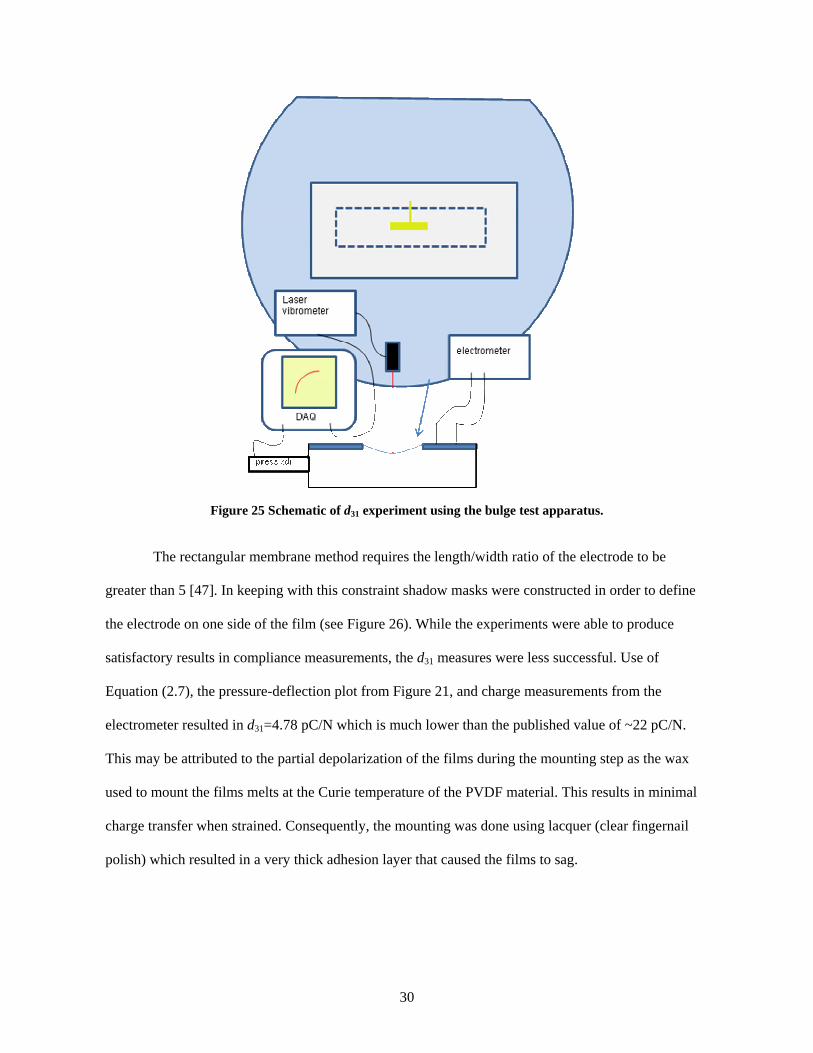
30
Figure 25 Schematic of d31 experiment using the bulge test apparatus.
The rectangular membrane method requires the length/width ratio of the electrode to be
greater than 5 [47]. In keeping with this constraint shadow masks were constructed in order to define
the electrode on one side of the film (see Figure 26). While the experiments were able to produce
satisfactory results in compliance measurements, the d31 measures were less successful. Use of
Equation (2.7), the pressure-deflection plot from Figure 21, and charge measurements from the
electrometer resulted in d31=4.78 pC/N which is much lower than the published value of ~22 pC/N.
This may be attributed to the partial depolarization of the films during the mounting step as the wax
used to mount the films melts at the Curie temperature of the PVDF material. This results in minimal
charge transfer when strained. Consequently, the mounting was done using lacquer (clear fingernail
polish) which resulted in a very thick adhesion layer that caused the films to sag.

31
Figure 26 Drawing of the electrode generated by the shadow mask used in the RMM d31 bulge test.
Another source of error arose with centering the laser vibrometer on the sample at a region
that would reflect an adequate signal. As the film was drawn down (with vacuum) into the puck
feature, the concave surface of the film would tend to reflect the laser signal away from the detector
reducing the signal strength. Additionally, the film surfaces were rough which caused the sputtered
gold electrode material to reflect poorly. Although this would provide a more precise measure of d31,
there are issues that must be overcome before the technique is effective.
2.6 Amplitude Measurements
This section describes an experiment to measure the displacements of the base motion of the
XMR and the displacement of the mass due to inertial motion. The displacements were measured
using a laser vibrometer with small pieces of a polished silicon wafer attached to the frame and mass
to act as reflectors. The XMR was driven at several resonant frequencies. Figure 27 shows the typical
results for a displacement versus acceleration experiment. In this particular case the difference
between the base and mass displacement is featured. This demonstrates the importance of operating an
oscillating device at resonance: the very small base motion causes very large excursions of the
resonant device. This results in larger strains in the compliant films which produce power in
proportion to the strain.

32
Figure 27 Typical plot showing the displacement vs. acceleration of the mass and base. The displacements between the mass and base differ by more than an order of magnitude.
Figure 28 shows the mass amplitude versus base acceleration at resonant frequencies of
152 Hz and 178 Hz. The interesting feature is the similarity in this plot to the power versus
acceleration plots shown elsewhere. This indicates that power roll-off and limitation is due to
reductions in vibration amplitude rather than a reduction in piezoelectric conversion.

33
Figure 28 Plot showing the measured mass amplitude vs. base acceleration of the XMR at resonant frequencies of 152 Hz and 178 Hz.
2.7 Damping
At one point, the question of the effect of a mass change on device performance at a constant
geometry was asked because of an assumption of constant mechanical damping. Before investing a lot
of time on design and manufacture for a variable mass XMR, the following experiment was conducted
to see if there was any change to the damping term.
Experiment The hypothesis is that with an unchanged geometry, the change in mass should not affect
mechanical damping. From the model development and mechanical analogue presented in Chapter 4,
and the equivalent electrical circuit parameter R, the damping term Rm is defined by the relationship
Rm=RΨ2, where Ψ, an electromechanical coupling term, is entirely composed of materials properties
and geometry terms.
An impedance sweep was measured on the XMR tuned nominally to 180 Hz. The sweep and
subsequent Matlab curve fit are shown Figure 29.

34
Figure 29 Initial impedance sweep, vs.Z f , (left) and curvefit (right) of impedance data of the XMR device nominally tuned to 180 Hz.
An easy method to add additional mass was to affix large binder clips onto the ends of the
XMR as shown in Figure 30. The total increase in mass was ~51.5 g. The clips were carefully attached
to ensure symmetry in order to minimize a significant change in the moment about the center of mass.
Figure 30 Image of the XMR device with binder clips attached.
After affixing the clips, another impedance sweep was taken. The results are shown in Figure 31.

35
Figure 31 Impedance sweep, vs.Z f , (left) and curvefit (right) of impedance data of the XMR device after the attachment of additional mass.
Comparing the plots in Figure 29 with the plots of Figure 31, the expected shift in frequency is
apparent. The fit (blue line) to the data (green line) seemed to be less satisfactory than fits conducted
on prior data sets, however it appeared to be consistent through both tests. The curve fit parameters are
shown in Table 2.
Table 2 Results from impedance sweep curve-fit.
Parameter XMR XMR + 52 g % ChangeC o 1.45E-10 1.45E-10 0.1R 4.25E+06 4.82E+06 13.4L 2.23E+05 2.95E+05 32.3
C m 3.58E-12 3.22E-12 -10.1k 2 0.024 0.022 -10.0f n 178 163 -8.3
Ψ (elec) 6.06E-04 6.74E-04 11.1s (elec) 1.03E+05 1.41E+05 37.4
R m (elec) 1.6 2.2 40.0Ψ (geo) 7.53E-04 7.53E-04 0.0s (geo) 1.31E+05 1.31E+05 0.0
R m (geo) 2.4 2.7 13.4C m (geo) 4.3E-12 4.3E-12 0.0
Q 58.4 62.9 7.8

36
(elec) indicates values from impedance data using Ψ2=m/L, s=Ψ2/Cm and Rm=RΨ2 (geo) indicates values from geometry using equations for s and Ψ below
Analysis The additional 52 g mass resulted in a 13% increase in R, and according to the mechanical-
electrical relationship from the model would suggest that the mechanical damping has increased. Now
consider the other terms, L and Cm. The mechanical analogs are 2L m= Ψ and 2mC s= Ψ . One
would expect a change to L, as the mass has changed but geometry has not, and results indicate a
change of 32%. The change to Cm is 10%, however one would not expect a change to this value as the
assumption was that s and Ψ would remain constant with geometry. The model equations for the terms
s and Ψ do not contain a mass term anywhere.
Frequency is calculated in the curve fit as n 1 2f LCπ= m , however frequency is also
defined as /f s m=n . From the assumption of constant device stiffness, s, the following
relationship should be true: 2 21 1 2 2f m f m= where the subscripts indicate the two test conditions. The
initial mass was 82 g. The additional mass added was 52 g, a 63% increase. Substituting values
produces:
( )( )2178 82 2.6E6= ,
( )( )2163 82 52 3.6E6+ = .
The significant inequality between the results strongly suggests that s did not remain constant with the
additional mass.
The following equations for s and Ψ are developed in detail in Chapter 4 but are placed here
for convenience:

37
3 2E 211 o
p
o
14 1 ,
1
whss L u
L
⎧ ⎫⎪ ⎪⎪ ⎪⎪ ⎪= −⎨ ⎬
⎡ ⎤⎪ ⎪⎛ ⎞⎢ ⎥+⎪ ⎪⎜ ⎟⎢ ⎥⎝ ⎠⎪ ⎪⎣ ⎦⎩ ⎭
and p311 2E 2
11 op
o
12 .
1
ud ws L u
L
Ψ =⎡ ⎤⎛ ⎞⎢ ⎥+ ⎜ ⎟⎢ ⎥⎝ ⎠⎣ ⎦
Using the mechanical analog from the impedance result (Ψ2=m/L) provides a means to calculate the
coupling term, Ψ. The result was used to find s and Rm. Inspection of the geometric equation for Ψ
indicates a dependence on geometric terms and materials properties, namely, compliance and
piezoelectric coefficient. The mass is known and the inductance is measured, however the coupling
term does not remain constant. The two terms that can change (because geometry did not change) in Ψ
are d31 and s11E. The calculation of Cm using Ψ and s from the electrical measures returns essentially
the measured value. This may be good in that Ψ and s are accurate or it may indicate that this
relationship is used to derive the values. Because the experiment was conducted with constant
geometry, using the relationship for 2mC s= Ψ and substituting the equations for Ψ and s above
should provide Cm~const(d312/s11
E).
The plot shown in Figure 32 is generated from measured data taken from the regular model
and the xs-model RXMR devices. In this case, the mass is constant with changes made to either the
geometry or the material. The difference in the mechanical damping term Rm is seen to vary with
changes in film thickness as well as film length. Film length (Lo) in the regular model is ~22 mm and
the xs-model has a film length of ~46 mm. While some of the data (119 µm regular) appear to be
linear, other data appear more clustered about a region. However a general trend seems to present
itself, damping is increased by both material thickness and geometry.

38
Figure 32 Mechanical damping Rm vs. up+uxs generated from data sets. Blue data are from 119 µm films, red data are from 28 µm films, diamonds are from a regular model device, triangles are from an xs-model device.
39
CHAPTER THREE
3 XMR BASICS
This chapter is principally a reproduction of a paper published in Smart Materials and Structures
(Morris, D.J., Youngsman, J.M., Anderson, M.J., and Bahr, D.F., A resonant-frequency tunable,
extensional mode piezoelectric vibration harvesting mechanism. Smart Materials and Structures, 2008.
17). Sections written by co-authors have been paraphrased but the structure and derivations are mostly
duplicated. The content has been expanded to address the additional figures that relate this work to
prior literature.
3.1 Introduction
The three principal methods of electromechanical energy conversion in vibration harvesting
devices are electrostatic, electromagnetic and piezoelectric. A number of reviews have been compiled
recently that present the theory and performance of these methods [8, 29, 49]. Electrostatic harvesters
have been demonstrated in different configurations [6]. Electromagnetic devices have been
successfully demonstrated for a variety of structures and designs [1, 3, 50]. Piezoelectric
configurations, principally fabricated as cantilevers of ceramic lead – zirconate – titanate (PZT), are
demonstrated in several publications; e.g. [6, 16, 51], and Kim et al present a unique compression
method with a piezoceramic structure [52].
Regardless of the particular electromechanical energy conversion technique, the entire
vibration harvesting device may be viewed as a simple oscillator (mass and spring), excited externally
by a vibration source, with mechanical and electrical dissipative paths. Electrical dissipation in this
sense is good; this is the power delivered to an electrical load or stored for use later. The mechanical
dissipation is the losses in the conversion due to friction, bending, or damping. It is generally
recognized that the most electrical power may be extracted when the mechanical device is at, or near,

40
resonance. Even good electromechanical converters convert a small fraction of the strain (piezoelectric
converters) or kinetic (electromagnetic or electrostatic converters) energy at each pass. Therefore, high
mechanical gain increases the effective transduction efficiency of input mechanical power to output
electrical power.
An array of simple cantilevers may have a difficult job harvesting power from what might be
viewed as a typical structural installation where a variety of frequencies are present. Even if each
cantilever was constructed for a particular frequency [49], such that it was harvesting at resonance,
there would be many devices operating at much less than optimal conditions. If a volume or weight
constraint is enforced, this configuration becomes even less appealing. It is possible to increase the
harvesting bandwidth of an individual cantilever such that a single or smaller array would capture
more vibration energy by introducing additional damping, but this also reduces the electrical output of
the device as the energy would be dissipated through the mechanical rather than the electrical path.
The issue of matching devices to environments leads to the interest in tunability. If a technique
were available to adjust a harvester to match the environment into which it is placed, power
production would occur at the efficient resonant frequency. This would allow less rigorous
manufacturing tolerances and the ability for a single device to be used in a variety of installations. It is
a straightforward extension to envision “smart” devices that could track the frequencies available in
the installation and adjust themselves to maximize power output.
The literature shows a few implementations of frequency tuning in resonant devices for vibration
harvesting. In general, the stiffness of the device is controlled as this is easier to implement than a
dynamic change in the effective mass. These methods fall into two main categories:
1. Control of the stiffness of a piezoelectric beam by adaptive capacitive loading or other electrical control schemes; for example, as in [6, 16, 17];
2. Bias loading of a piezoelectric beam, which can decrease the stiffness by application of a compressive end load [19] or, application of magnetic forces to increase or decrease the beam stiffness [20].

41
Another class of wide band vibration harvesting mechanisms decouples the vibration frequency
from the resonant frequency of the piezoelectric element by pulse-excitation of a high-natural-
frequency generator by a low-frequency resonator [21, 23].
In this chapter a new mechanism that is capable of resonant frequency tuning will be detailed.
The device can utilize any piezoelectric material or structure capable of supporting a tensile load. For
simplicity the initial device designs utilize polyvinylidene fluoride (PVDF) films of varying
thicknesses, but the theory outlined is applicable to other families of materials, for example,
piezoceramics on metal foils. The device couples two nonlinear spring elements into a configuration
that becomes an oscillator with wider ranges of linear motion. The spring elements, in this case PVDF
films, are affixed on one end to a central mass and on the other end, to an adjustable frame element.
By changing the length of the frame element, the effective stiffness of the spring element is changed
which alters the resonant frequency of the system. Electrical power is observed to scale with
acceleration as expected, however it is relatively insensitive to changes in the natural frequency.
3.2 The Extensional Mode Resonator
In this chapter the device described utilizes stretching rather than bending of the piezoelectric
element. The device is constructed of films or membranes which by definition cannot support bending
or compressive loads. Consider a film element of width, w, length 2l, and thickness h, firmly anchored
to a frame. The force, F, required to deflect the center of the single film element a distance, u, shown
in Figure 33(a) can be described by the following equation for small excursions where u/l << 1
33 .EwhF u
l= (3.1)
This exhibits a cubic relationship between force and displacement.
Now if two identical films are attached with a rigid link of length 2up=u1+u2 as shown in
Figure 33(b) the films act as spring elements and the structure will be in a state of static equilibrium. A
force balance equation can be written as

42
3 3TOT 1 23 3 0,Ewh EwhF u u
l l= + = (3.2)
and recognizing in the presented configuration u1 is opposite in sign to u2 and consequently equal to
up. Finally introduce an arbitrary excursion ∆u to the structure. This results in a force balance equation
written as
( ) ( )3 3
TOT p p3 3 ,Ewh EwhF u u u ul l
= + ∆ + − + ∆ (3.3)
which simplifies to
( )2 3TOT p3 6 2 .EwhF u u u
l= ∆ + ∆ (3.4)
This demonstrates a force-deflection relationship of the structure with both linear and cubic terms in
∆u. For sufficiently small displacements of ∆u, the cubic portion contributes very little to the total
force, FTOT, and can be neglected. The effective stiffness of the structure can be found through the
following equation
Figure 33 (a)Schematic of the displacement u of a rectangular string of non-deformed length 2l, thickness hand width w (out of the plane of the figure) at the center by a force F. (b) Pre-tensioning two extensional elements by a rigid link of length 2up. (c) Displacement of the link by an external force F by an amount ∆u.

43
( )2TOTp3
d 6 .d
F Ewhk uu l
= ≈∆
(3.5)
This demonstrates that a geometric change to the structure should allow an increase or decrease in the
force required to displace the link. Substitution of Equation (3.5) into Equation (1.1) allows the
derivation of an equation that demonstrates a linear relationship of frequency to the geometric change
of the spring elements.
N p 3
1 62
Ewhf umlπ
= (3.6)
The next section describes the construction and testing of a device to validate the equations presented
to this point.
3.3 Prototype Device Fabrication and Experimental Measures
For proof-of-concept testing the first prototype of the XMR used a full circular diaphragm
geometry made from metalized 28 µm-thick piezoelectric polyvinylidene fluoride (PVDF)
(Measurement Specialties, Inc), and a seismic mass largely constructed from an alloy of 90 %
tungsten, 6 % copper, and 4 % nickel (Marketech International). The tungsten alloy has a density of
17,000 kg m-3, which is close to the density of pure tungsten (19,300 kg m-3) but is easy to machine
with conventional tooling. The total live mass was 26.4 g. Other rigid parts of the XMR were
constructed of brass. The PVDF was glued to the clamping rings and attached to both sides of the
seismic mass with nylon screws. The W-alloy and brass components were electrically isolated from
the metalized PVDF film by applying a lacquer coating where they might contact the PVDF, and
etching the electrodes from the PVDF using a peroxy-sulfuric acid solution. The electrodes may also
be etched using a ferric chloride solution. The electromechanical properties of the PVDF, as reported
by the manufacturer, are d31 = 23 pC N-1, ε = 106-113 pF m-1, and E = 2-4 GPa; the films were chosen
for ease of use in verification of the model and initial device construction, and should not be
considered as either upper or lower bounds on the range of materials that could be used in this device.

44
The PVDF elements were suspended at the center with flanged brass spools. The rigid link
between the spools is an 8-32 screw, the effective length of which may be changed by turning the
screw relative to the spools. This is the mechanism by which up, and therefore the resonant frequency,
is controlled. Figure 34(a) is a cross section view of the XMR detailing the relationship between the
components. Figure 34(b) a photograph of the assembled XMR in preparation for testing. The volume
of the XMR (excluding testing fixtures) is about 10 cm3 (0.6 in3).
Figure 34 (a) Section view of the XMR (b) Photograph of an assembled XMR device
Figure 35 is a cross-sectional schematic that demonstrates the operation of the XMR. In this figure, the
base to which the device is attached is considered the reference frame and is rigidly attached to the
page. The membrane suspension spools are also rigidly attached to the base. Vibration excitation of
the base induces motion of the seismic mass relative to the base. This in turn causes each piezoelectric
membrane to alternately lengthen and shorten. Electrodes on both sides of the piezoelectric material
collect charge developed through the direct piezoelectric effect.
PVDF
Mass
Adjustment screw
Clamp ring
Base

45
Seismic mass Motion of seismic mass relative to base
Base
Preloading adjustment
Shortened membrane
Lengthened membrane
Figure 35 Cross-sectional schematic of the XMR device driven by base excitation. In this schematic, the seismic mass has moved upwards relative to the base, causing the top piezoelectric membrane to shorten and the bottom membrane to lengthen. Continued vibratory motion causes the membranes to alternately lengthen and shorten [24].
The XMR was mounted to a vibration table (Brüel and Kjaer 4801) for testing. The driving
signal was typically white noise (to observe a frequency spectrum) or a sine wave from the signal
source on a dynamic signal analyzer (DSA) (Agilent 35670A). The open-circuit voltage from the
XMR, and an accelerometer that was mounted to the vibration table, were input to the DSA. The data
were collected using either an oscilloscope (Tektronix TDS 2002) or the DSA. A convenient method
of characterizing the spectrum of dynamic behavior is the frequency response function (FRF), defined
here as the open circuit voltage across one or both of the piezoelectric membranes divided by the
acceleration measured from the vibration table.
3.4 Frequency Tunability
Figure 36 is a plot of several FRFs acquired from the XMR in open-circuit conditions after
changing the pretension displacement between three tuning screw positions in random order. Position
2 was the initial point. Position 1 had an up of 0.1 mm less than Position 2 and Position 3 had an up of
0.2 mm greater than Position 2. In general the resonant frequency was repeatable within the ability to
reposition the tuning screw to the same location. The ability to reproduce the specific frequency of
interest was possible to within 1% of the frequency; this is limited by the sensitivity of the adjustment
screw used in the current study and not a fundamental limit on the device. Long term static loads with

46
this level of pre-tension did not cause the device resonant frequency to drift. In a complementary
experiment, an XMR was tuned to a resonant frequency that was measured to be 81.5 Hz. The XMR
was then driven at this frequency for four hours with a 9 m/s2 acceleration amplitude. Every hour the
resonant frequency of the XMR was measured using an impedance sweep technique [53], and found to
be within the experimental uncertainty of the measurement (0.3 Hz). The prototype system
demonstrated the ability to adjust to and maintain a specific resonant frequency. Furthermore, the
voltage to acceleration ratio at resonance is effectively constant, even when doubled in frequency.
Figure 36 Frequency response functions from a frequency-tuning experiment in which each symbol indicates the same adjustment position. Different experiments at each adjustment position have different shading. The adjustment was varied between the three positions in a random sequence. This demonstrates the reproducibility of the frequency tuning mechanism.
A second resonant frequency tuning experiment was undertaken to examine the prediction of
linearity of frequency to geometric changes to the device. The results in Figure 37 provide support for
the assumption presented in Equation (3.6). The XMR was adjusted through a range of preloads which
varied the dimension up by approximately 1.25 mm which resulted in resonant frequencies that ranged
from 80 Hz to 235 Hz. The red line represents a least squares linear fit of the data that lies within a
Position 1 Position 2 Position 3

47
95% confidence interval. This broad range of frequencies encompasses almost the entire spectrum of
low level vibration sources suitable for energy harvesting as reported by Roundy [29]. By comparison
this range of tuning, on the order of 66% calculated as ( )max min max/f f f− , is far greater than others
reported in the literature.
!"!!
Figure 37 Resonant frequency, determined by the frequency response function, as a function of relative preloading displacement. The placement of the preloading screw at 212 Hz is an arbitrary datum. The solid line is a least-squares linear fit, and the dashed lines indicate a 95 % confidence interval [24].
Leland and Wright achieved a reduction in resonant frequency from 250 Hz to 200 Hz and
from 190 Hz to 160 Hz (two different seismic masses) by applying a compressive axial load to a beam
that supported a seismic mass midspan as shown in Figure 38 [19]. The lower limit occurred at the
buckling point of the column due to the large loads required, up to 65 N. They report a tuning range of
20% for a 7.1 g mass and 16% for a 12.2 g mass.

48
Figure 38 Compressive beam technique (a) schematic of technique (b) device under test [19].
Challa et al [20] has shown a technique using permanent magnets attached to a cantilever
harvester and the frame to either increase or decrease the resonant frequency. The adjustment depends
on the orientation of the poles of the magnets. Like poles cause a relative increase of the beam
stiffness and consequently an increase in the resonant frequency while opposing poles reduce the
stiffness but also present a problem of attachment in the event of over-travel by the beam. The
cantilever/mass assembly has a natural frequency of 26.2 Hz. Through application of the magnets and
adjustment of the separation distance dx of the magnets, they were able to tune the frequency between
22 Hz and 32 Hz. Using the same calculation above, this results in a reduction of 31%.
Figure 39 Magnetic assist by Challa et al (a) magnet configuration that increases the effective stiffness of the beam (b) magnet configuration that decreases the effective stiffness of the beam. (c) Device schematic showing positions of components [20].
Hu et al [54] describes a model for a piezoelectric cantilever capable of applying a tensile or
compressive loads to the end much like the device demonstrated by Leland and Wright. The model
(c)

49
demonstrates that if such a device were constructed it would have a very broad tuning range, 60 Hz to
170 Hz, with power densities on the order of 40 µW/cm3. Frequency tuning is accomplished by
adjusting a screw that is integrated or coaxial with the support layer in a bimorph piezoelectric
cantilever. Figure 40 shows the authors suggested design.
Figure 40 Schematic of Hu et al method to load a bimorph cantilever [54].
3.5 Power Results of the XMR
Figure 41 shows the power output of the original prototype device at several frequencies and
accelerations. The power is calculated as 2rms LP V R= where RL is a fixed load resistance of
490 kΩ. It should be noted that the load was not impedance matched and only a single film was
producing power. With both films operating, the power doubles. Impedance matching, where the load
resistance is equal to the internal resistance of the piezoelectric device will allow the device to produce
its maximum power.

50
Figure 41 Power vs. acceleration for the prototype XMR.
Initial results at the lower acceleration amplitudes indicate a lesser dependence on frequency.
The results in Figure 42 show the data from the linear region of the power-acceleration relationship. A
statistical regression was performed on the data in this plot using Minitab software (State College, Pa.)
to determine the primary influence on power production. The two inputs evaluated are acceleration
amplitude and resonant frequency. The results report a p-value which is a measure of probability that a
hypothesis of a particular regression coefficient should be rejected. Typically, p=0.05 is taken as the
boundary between large and small. Regression of the data in Figure 42 to a model
2log log( ) log( )P K Aβ= + (3.7)
where log(K) and β are arbitrary constants returns log(K)=0.627 and β=0.818 with p=0.000 for both
terms. This implies that the terms are likely significant. Now if the data are regressed to
2Nlog log( ) log( ) log( )P K f Aα β= + + (3.8)
where α is a constant for the log(fN) regression term relating to resonant frequency, the results are p-
values of p=0.000 for β, and p=0.427 for α. This means that the power output term may be

51
significantly related to the acceleration amplitude but not significantly related to the resonant
frequency [24].
Figure 42 Power vs. acceleration of the prototype XMR at low acceleration amplitudes.
3.6 Conclusions
The extensional mode resonator (XMR) described in this chapter exploits the nonlinear force-
deflection characteristics of a membrane to create a highly tunable piezoelectric vibration harvesting
device. By rigidly coupling two piezoelectric membranes in the manner described, the nonlinearities
cancel to create a linear spring with a highly variable spring constant. A piezoelectric vibration
harvesting device with a repeatable frequency adjustment range greater than 150 Hz has been
demonstrated. The large natural frequency adjustment range is beneficial in that a single vibration
harvester model can generate substantial power in many different vibration environments. Analysis of
power output demonstrates a strong dependence on acceleration amplitude with less dependence upon
resonant frequency.

52
CHAPTER FOUR
4 MODEL DEVELOPMENT OF THE RXMR
This chapter is principally a reproduction of a paper submitted for publication in Journal of Sound and
Vibration in 2009. Sections written by co-authors T. Luedeman, D. Morris, M. Anderson, and D. Bahr,
have been paraphrased where possible but the structure and derivations are mostly duplicated.
4.1 Introduction
Improvements in wireless communication and sensing techniques, along with the reduction of
power consumption in current microelectronics are driving demand for structural health monitoring
systems. Although power consumption is low, battery life remains a critical factor in installation of
distributed sensor networks. Because battery exchange requires considerable manpower, techniques
are under investigation that can charge batteries or alternatively super capacitors as a means to extend
the service life of installed networks. A larger concern is the installation that is either dangerous or no
longer accessible for battery exchange. Solar generated power is ubiquitous, but is not a universal
solution. A solution is required for installations that may not have or may not want solar exposure.
Vibrations are available in many instances and can provide the critical energy input for the
piezoelectric class of materials. Researchers are investigating vibration harvesting utilizing various
self energizing techniques including electromagnetic in both a cantilever configuration [1-3] and
single membrane form [4, 5], and piezoelectric, principally as cantilevers [6, 7]. A number of recent
reviews discuss harvesting theory, techniques, and performance [8-11, 55].
A critical issue with most resonating harvesters is their best performance occurs at a single or
very narrow frequency range. Therefore, many devices must be designed for and limited to a known
environment. Adjustable resonant tuning provides flexibility in a device and the opportunity to

53
maximize power generation. Literature shows limited cases of resonant tuning and can be described as
external electrical control [16, 17], beam compression techniques [18, 19, 54], beam stiffness change
through piezoelectric effect [18], beam stiffness change through magnetic field application [20],
decoupling [21], cantilever arrays [22], or frequency rectification [23].
An issue with the cantilever design is the reduction in power output as the driving frequency
increases. An accepted model predicting the maximum power of a cantilever harvester as postulated
by a number of researchers [1, 8, 11, 29, 42] is shown in Eq. (4.1) and a conditional form, as suggested
by Morris et al. [24] is written as Eq. (4.2)
2E
2T4
m Aζωζ
Π =( )
2 2E
2 2E E M M
,2 2
b m Ab b b b
=+ +
(4.1)(4.2)
where A is the acceleration amplitude, ζE and ζT are the electrical and total dimensionless damping
coefficients, and bE and bM are the electrical and mechanical damping coefficients. The equation
assumes that the natural frequency, ωn, equals the driving frequency, ω. From Eq. (4.1) it is apparent
that as the driving frequency increases, the power generated is reduced if the damping coefficients
remain constant with frequency. The conditions of Eq. (4.2) assume the damping terms bE and bM
remain constant with changes in device stiffness. This removes the dependence on frequency for
electrical power generation.
The extensional mode resonator (XMR) [24] is constructed of piezoelectric films, in this case
polyvinylidene fluoride (PVDF), that suspend a mass to a rigid frame. As the frame vibrates, the
compliance of the films permits the mass to oscillate about a neutral axis which alternately stretches
the films. The alternating strain cycle applied to the films generates electricity through the direct
piezoelectric effect. The unique geometry of the XMR permits simple adjustability of the resonant
frequency through a change in stiffness rather than a change in mass. Initial experiments with the
XMR device appear weakly dependant upon resonant frequency and more strongly affected by
mechanical damping (bM in Eq. (4.2)).

54
An advantage of the XMR design (Figure 43) is the ability to utilize stretching rather than
bending mode for generating the piezoelectric effect. The initial prototype device presented in the
previous chapter utilized circular membranes. During the development of the following model it was
determined that although the circular XMR model is more structurally stable, it had lower power
output due to a strain gradient as a result of its circular design. In the case of the rectangular version,
all strains are uniaxial and uniform. Because there is no strain gradient as in the circular XMR or a
cantilever [6], the entire active area of the films produce power effectively. The implications of
geometry changes to the device stiffness and frequency are shown in the following model section
followed by verification of the model with an experimental prototype device.
Figure 43 Schematic for mechanical function of the XMR device.

55
Figure 44 Schematic for electrical function of the device.
4.2 Dynamic Model
Consider the schematic diagrams of the eXtentional Mode Resonator shown in Figure 43 and
Figure 44. They illustrate the mechanical and electrical function of the device. As shown in Figure 43,
the device consists of a moving mass m and adjustable frame. Four PVDF films, of unstretched length
Lo, width w (into the plane of the figure), and thickness h are fixed to the moving mass and the central
hub of the frame. The central hubs are moved vertically a distance up from the moving mass to preload
the films and deform them to the dimension L . The frame is moved at a specified inertial acceleration
u , while the inertial displacement of the mass is z, and the displacement of the mass relative to the
moving frame is ∆u. While m executes relative movements ∆u, the instantaneous length L of each film
is L L L= + ∆ , where ∆L is the stretch of each film caused by the movements ∆u. In Figure 44 the
electrical function of the upper and lower films are shown symbolically. The top and bottom
electrodes on the upper and lower sections are connected, so as to form the potentials ∆Vu and ∆Vl
respectively. The polarity of the upper and lower films are indicated by “+” and “-”, where the polarity
is referenced to the free charge attracted to the electrode. The currents iu and il flow into the top

56
electrodes of the upper and lower films. A load resistor RL is placed as shown to model harvesting of
electrical energy, and the remaining electrodes will be connected such that iu=il.
The objective is to develop a model that will predict the time-averaged power Π dissipated in
a resistor placed across the electrodes of the XMR given a specified acceleration u . In what follows,
Newton’s second law will be derived for the vertical motion of m, and the electromechanical coupling
of the PVDF film to a load resistor placed across the electrodes will be determined.
To derive the mechanical response of the device, consider the free-body diagram of the mass
in the deflected condition shown in Figure 45. Neglecting gravity, the only forces on the mass
originate from the stretching of each PVDF film. Denote N as the axial force of a PVDF film on m,
and Fv as the vertical component of the axial force N.
Figure 45 A free-body diagram for the mass m.
Furthermore, the vertical reactions are subdivided in Fv
+ and Fv- depending upon whether they
originate from the upper or lower films respectively. The force Fv can be computed from Fv=Ncosα,
where the angle α is subscripted as αu and αl for the upper and lower films shown in Figure 43 and
Figure 45. The axial force N can be computed from the constitutive equations for the film [56]
1 31 3 11 1S d E s T= − + E , (4.3)

57
3 33 3 31 1D E d Tε= −T , (4.4)
where S, T, E, and D are strain, stress, electric field and electric displacement; d31, 11sE , and 33ε T are the
piezoelectric coefficient, mechanical compliance and electric permittivity; the 1-direction is along the
film axis and the 3-direction is in the film thickness direction. In Equations (4.3) and (4.4), the upper
films are assumed to be oriented such that a release in tension associated with positive movements ∆u
of m cause a positive voltage at the top electrode, consistent with Figure 44. Consequently, the
piezoelectric coefficient d31 is taken to be negative. The constitutive model, Equations (4.3) and (4.4),
assumes that the stress in the 2-direction is zero (T2=0), and that the films are free to contract in the 2-
direction. This is a simplifying assumption in the model, and its quantitative effect will be neglected at
this point in time. Given that T1=N/wh because a tension on an upper film is a force Fv in the opposite
direction on m, Fv=Ncosα, S1=∆L/Lo, and 30
hV E dz∆ = −∫ , Equation (4.3) can be rewritten for the
upper and lower films as
31
11 11
cos coswh L d wF Vs L s
α α+ ∆= + ∆v u u uE E
o (4.5)
31
11 11
cos coswh L d wF Vs L s
α α− ∆= − ∆v l l lE E
o (4.6)
The component of the force Fv- induced by the voltage ∆Vl on m from the lower film is negative
because the polarity of the lower films are opposite that of the upper films. To obtain a linear model, it
is assumed that ∆u of m is small, and linearization of Equations (4.5) and (4.6) results in
311 2 3 2 1 22 2 2
11 11 11
1 1 11 1
1 1 1
u uwh wh d wF u V
s L s L s Lu u uL L L
+ = − − − ∆ − ∆
+ + +
⎧ ⎫ ⎧ ⎫⎪ ⎪ ⎪ ⎪⎪ ⎪ ⎪ ⎪⎪ ⎪ ⎪ ⎪⎨ ⎬ ⎨ ⎬
⎡ ⎤ ⎡ ⎤ ⎡ ⎤⎪ ⎪ ⎪ ⎪⎛ ⎞ ⎛ ⎞ ⎛ ⎞⎢ ⎥ ⎢ ⎥ ⎢ ⎥⎪ ⎪ ⎪ ⎪⎜ ⎟ ⎜ ⎟ ⎜ ⎟
⎝ ⎠ ⎝ ⎠ ⎝ ⎠⎢ ⎥ ⎢ ⎥ ⎢ ⎥⎪ ⎪ ⎪ ⎪⎣ ⎦ ⎣ ⎦ ⎣ ⎦⎩ ⎭ ⎩ ⎭
p p
v uE E Eo o o
p p p
o o o
, (4.7)

58
311 2 3 2 1 22 2 2
11 11 11
1 1 11 1
1 1 1
.u uwh wh d w
F u Vs L s L s Lu u u
L L L
− = − − − − ∆ − ∆
+ + +
⎧ ⎫ ⎧ ⎫⎪ ⎪ ⎪ ⎪⎪ ⎪ ⎪ ⎪⎪ ⎪ ⎪ ⎪⎨ ⎬ ⎨ ⎬
⎡ ⎤ ⎡ ⎤ ⎡ ⎤⎪ ⎪ ⎪ ⎪⎛ ⎞ ⎛ ⎞ ⎛ ⎞⎢ ⎥ ⎢ ⎥ ⎢ ⎥⎪ ⎪ ⎪ ⎪⎜ ⎟ ⎜ ⎟ ⎜ ⎟
⎝ ⎠ ⎝ ⎠ ⎝ ⎠⎢ ⎥ ⎢ ⎥ ⎢ ⎥⎪ ⎪ ⎪ ⎪⎣ ⎦ ⎣ ⎦ ⎣ ⎦⎩ ⎭ ⎩ ⎭
p p
v lE E Eo o o
p p p
o o o
(4.8)
The terms in Equations (4.7) and (4.8) above are caused by static extension of the films,
displacements ∆u caused by movement of the mass, and the voltages ∆Vu and ∆Vl induced across the
electrodes of the upper and lower films. The total vertical force F on m from all four films then is
2 2F F F s u V V+ −= + = − ∆ − Ψ∆ − Ψ∆v v u l , (4.9)
where
3 2211
14 1
1
whss L u
L
⎧ ⎫⎪ ⎪⎪ ⎪⎪ ⎪= −⎨ ⎬
⎡ ⎤⎪ ⎪⎛ ⎞⎢ ⎥+⎪ ⎪⎜ ⎟⎢ ⎥⎝ ⎠⎪ ⎪⎣ ⎦⎩ ⎭
Eo
p
o
(4.10)
311 22
11
12
1
ud ws L u
L
Ψ =⎡ ⎤⎛ ⎞⎢ ⎥+ ⎜ ⎟⎢ ⎥⎝ ⎠⎣ ⎦
pE
op
o
. (4.11)
Physically, s is a mechanical stiffness, and Ψ is a coupling coefficient with units of N/V.
There are two components of s, one given by the extensional stiffness of the four films, and the other
being a geometric dilution parameterized by the ratio up/Lo. Similarly, Ψ consists of a component that
would be expected from extensional strains, and a geometric dilution. Newton’s second law for the
motion of the mass is
( )F R z u mz− − =m , (4.12)

59
where Rm is a coefficient of mechanical damping. Using the fact that z=u+∆u, letting u =-A(t), and
using Equation (4.9) for F, Newton’s law, Equation (4.12), for m becomes
( ).m u R u s u V V mA t∆ + ∆ + ∆ + Ψ∆ + Ψ∆ =m u l (4.13)
To derive the electrical response of the device, voltage-current laws are derived for the upper
and lower films shown in Figure 44. Starting with one of the upper films, elimination of the stress T1
from Equations (4.3) and (4.4) gives
231 31
3 33 3 111 33 11
1 d dD E Ss s
εε
⎛ ⎞= − −⎜ ⎟
⎝ ⎠T
E T E . (4.14)
Upon integrating ( )0
hdz∫ , using the fact that 30
hV E dz∆ = −∫u , 3 0D z∂ ∂ = within the piezoelectric
material, and 1S L L= ∆ o , Equation (4.14) becomes
231 31
3 3311 33 11
1 d d LhD V hs s L
εε
⎛ ⎞ ∆= − − ∆ −⎜ ⎟
⎝ ⎠T
uE T Eo
. (4.15)
Next, integrate over a volume of infinitesimal thickness enclosing the interface between the electrode
and the piezoelectric film. This operation converts Equation (4.15) to
231 31
3 3311 33 11
1 d d LwL hD wL V wL hs s L
εε
⎛ ⎞ ∆= − − ∆ +⎜ ⎟
⎝ ⎠T
o o u oE T Eo
. (4.16)
To obtain a linear model for the upper films, ∆L/Lo is approximated for small motions ∆u, the quantity
wLoD3 is equated to the total free charge Q attracted to the electrode, and Equation (4.16) is multiplied
by two to reflect the fact that the two top and bottom electrodes are common. Additionally, it is
assumed that charge caused by static deformation has been dissipated. One then obtains
Q C V u− = − ∆ + Ψ∆u u , (4.17)
where Qu is the total free charge attracted to the top electrodes on the upper films and

60
231
3311 33
12
d wLs
Ch
εε
⎛ ⎞−⎜ ⎟
⎝ ⎠=
ToE T
. (4.18)
The derivation for the lower films is similar, only that the polarity orientation of the film is reversed,
and positive movements of the mass ∆u lead to extensional strains. For the lower films, the voltage-
current law then is
Q C V u− = − ∆ + Ψ∆l l . (4.19)
As a final step, the circuit is completed by connecting the bottom electrode on the upper films to the
top electrodes of the lower films. Then, iu=il and V=∆Vu+∆Vl=-iuRL, and the time derivative of the
circuit equations for the upper and lower films are summed to obtain
VC V uR
= − + Ψ∆oL
, (4.20)
where
231
3311 33
1
2
d wLsCCh
εε
⎛ ⎞−⎜ ⎟
⎝ ⎠= =
ToE T
o . (4.21)
Equations (4.13) and (4.20) constitute a model for the device, where the acceleration of the frame A(t)
is the input, and there are two equations for the unknowns V and ∆u.
4.3 Electric Circuit Analysis and Energy Harvesting Capability
The model for the XMR device has a circuit analogy that is useful for analysis of power
harvesting capability. Consider the circuit diagram shown in Figure 46. With the definitions of voltage
mA(t)/Ψ and current Ψ u∆ , and the components R=Rm/Ψ2, L=m/Ψ2, and C=Ψ2/s, the circuit shown in
Figure 46 can be verified to have the same governing equations as Equations (4.13) and (4.20).

61
Figure 46 Equivalent circuit diagram for the device (Equations (4.13) and (4.20)).
Furthermore, the natural frequency of the RLC circuit is
3 2211
1 1 14 1
1
s whm m s LLC u
L
ω
⎧ ⎫⎪ ⎪⎪ ⎪⎪ ⎪= = = −⎨ ⎬
⎡ ⎤⎪ ⎪⎛ ⎞⎢ ⎥+⎪ ⎪⎜ ⎟⎢ ⎥⎝ ⎠⎪ ⎪⎣ ⎦⎩ ⎭
n Eo
p
o
, (4.22)
and the quality factor Q is
3 2211
1 14 1
1
ms whQ mR R s L u
L
⎧ ⎫⎪ ⎪⎪ ⎪⎪ ⎪= = −⎨ ⎬
⎡ ⎤⎪ ⎪⎛ ⎞⎢ ⎥+⎪ ⎪⎜ ⎟⎢ ⎥⎝ ⎠⎪ ⎪⎣ ⎦⎩ ⎭
Em m o
p
o
. (4.23)
Given a harmonic frame acceleration of amplitude A, it is necessary to specify the optimal frequency
of operation and load resistance RL. It has been shown [57, 58] that in the limit of low damping,
optimal power production is obtained at two frequencies, the resonance frequency ωn given by
Equation (4.22) and the anti-resonance frequency. When damping becomes larger and exceeds a
particular limit, called the bifurcation damping ratio [58] there is a single frequency for optimal power
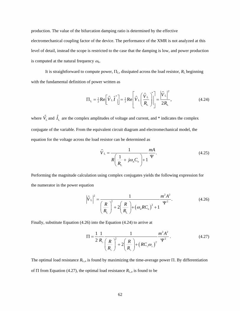
62
production. The value of the bifurcation damping ratio is determined by the effective
electromechanical coupling factor of the device. The performance of the XMR is not analyzed at this
level of detail, instead the scope is restricted to the case that the damping is low, and power production
is computed at the natural frequency ωn.
It is straightforward to compute power, ΠL, dissipated across the load resistor, RL beginning
with the fundamental definition of power written as
2*L* L1 1
L LL 2 2L L
Re Re ,2
VVV I VR R
⎡ ⎤⎛ ⎞⎡ ⎤ ⎢ ⎥Π = = =⎜ ⎟⎢ ⎥ ⎜ ⎟⎣ ⎦ ⎢ ⎥⎝ ⎠⎣ ⎦ (4.24)
where LV and LI are the complex amplitudes of voltage and current, and * indicates the complex
conjugate of the variable. From the equivalent circuit diagram and electromechanical model, the
equation for the voltage across the load resistor can be determined as
L
n oL
1 .1 1
mAVR j C
Rω
=Ψ⎛ ⎞
+ +⎜ ⎟⎝ ⎠
(4.25)
Performing the magnitude calculation using complex conjugates yields the following expression for
the numerator in the power equation
( )
2 22L 2 2
2o
L L
1 .
2 1n
m AVR R RCR R
ω
=Ψ⎛ ⎞ ⎛ ⎞
+ + +⎜ ⎟ ⎜ ⎟⎝ ⎠ ⎝ ⎠
(4.26)
Finally, substitute Equation (4.26) into the Equation (4.24) to arrive at
( )
2 2
2 22
1 1 12
2
m AR R R RC
R Rω
Π =Ψ⎛ ⎞ ⎛ ⎞
+ +⎜ ⎟ ⎜ ⎟⎝ ⎠ ⎝ ⎠
L
o nL L
. (4.27)
The optimal load resistance RL,o is found by maximizing the time-average power Π. By differentiation
of Π from Equation (4.27), the optimal load resistance RL,o is found to be

63
( )21
RRRC ω
=+
L,o
o n
. (4.28)
Given an optimal load resistance RL,o specified by Equation (4.28), the corresponding optimal time-
averaged power dissipation Πo from Equation (4.27) will be
( )2 2
2
1 14 1 1
m AR RC ω
Π =+ +
om
o n
. (4.29)
4.4 Prototype Device
A prototype XMR was fabricated for experimental verification of the model. The active
components of the device occupied a net volume of 21 cm3. The total live mass of the device was
82.3 g. Commercially available PVDF film (Measurement Specialties, Inc.) was used as the
piezoelectric element. Properties of the film provided by the manufacturer and other device constants
are contained in Table 3.
Table 3 Device geometry constants and PVDF film properties.
m [g] 82.3 Lo [mm] 22 w [mm] 23.95 h [µm] 119
s11E [m2/N] 3.65E-10
d31 [C/N] -2.30E-11
ε33T [C/V/m] 1.10E-10 k31 [%] 1.15E-01
4.5 Electrical Impedance
Electrical impedance experiments were conducted with an Agilent 4294A precision
impedance analyzer to determine the circuit parameters Co, R, L, C and k2. The electromechanical
coupling coefficient k2 is defined as the ratio of energy converted by the system divided by the energy
input into the system. The impedance sweep data (Figure 47) was curve fit using a least squares fit in

64
which variables Co, R, L, and C were allowed to change. The mechanical damping Rm was calculated
using the measured R from the impedance sweep, Equation (4.11), and the relationship Rm=RΨ2.
Results from the impedance sweep were also used to find the optimal load resistance RL,o in order to
achieve a matched impedance power experiment. The films were connected in series so that
measurements captured the values of the device rather than the individual film elements. An electrical
impedance measurement was conducted at each tension screw setting up, as the circuit parameters
depended upon the device geometry as discussed in Section 4.2 Dynamic Model.
Figure 47 Measurement of electrical impedance and curve fit for circuit parameters R, L, C, Co and k2.
4.6 Mechanical Vibration and Power Output
The schematic for the power measurement experiment is detailed in Figure 48. The XMR
device was mounted to a MB Electronics EA1250 vibration head driven with a MB Electronics 2120
amplifier. The input signal to the amplifier (both white noise and fixed sine) was generated by an
Agilent 35670A Dynamic Signal Analyzer (DSA). Accelerations were measured with a Bruel & Kjaer
Type 4395 accelerometer mounted to the vibration head. The impedance matched resistive load was

65
provided by an AEMC BR07 decade resistance box. Measurements were conducted at room
temperature. Temperature effects were observed during other extended run experiments and caused
~10% reduction in power when the room temperature increased by ~5°C but were not observed in the
short time span of the present experiments.
Figure 48 Apparatus used to perform power output experiment from a controlled vibration source.
The typical power measurement series was conducted by first exciting the XMR with white
noise in order to determine the resonant frequency. In addition to providing the source signal, the DSA
was used to capture the XMR and accelerometer output voltages and to plot the transfer function of
mechanical excitation shown in Figure 49. In this experiment the transfer function was defined as the
output RMS open circuit voltage of the XMR divided by the acceleration. Open circuit condition
refers to the absence of an electrical load across the film elements. The resonant frequency was
identified by the maximum in the transfer function. Once the resonant frequency was found, the XMR
was excited with a fixed sine signal at that resonant frequency at multiple accelerations. A feature of
the DSA enables the use of measurement averaging (in this case, 50 measurements) to improve the
resolution in VRMS for each acceleration setting. Power was calculated from 2P V R= RMS L where RL is
the total load resistance of the system (load from the decade box parallel to load from the DSA). When
all the desired measurements were collected, the XMR was tuned to a new resonant frequency by
adjusting the tension screws. This step changed the up position and the initial tension in the films. For

66
each position up, a new impedance measurement was conducted. Once the impedance measure was
made, the power experiment was repeated.
Figure 49 Transfer function vs. frequency of the XMR device. Peak indicates the resonant frequency of the oscillator.
4.7 Results
In this section, results of impedance and mechanical vibration measurements as described in
Sections 4.5 and 4.6 are presented. These measurements allow comparison of measured and
theoretically predicted device parameters and power output. A discussion of properties of the device as
predicted by the theoretical model follows in Section 4.8.
4.7.1 Impedance Tests and Device Parameters Table 4 provides a comparison of the XMR properties obtained in the impedance experiment
with the values determined from the theoretical model. The model provides the fundamental values
from geometry and materials properties to calculate the terms in Table 4 using the additional
relationships C=Ψ2/s, L=Ψ2/m, k2=C/(C+Co),and fn=ωn/2π. The geometric term up was selected to
obtain nominal natural frequencies of fn=120 Hz, 150 Hz, and 180 Hz, shown in Table 4.

67
Table 4 Configuration, impedance measurements, and theoretical predictions for nominal natural frequency of fn=120 Hz, 150 Hz, and 180 Hz. (119 µm film)
Consider the measurements and predictions contained in Table 4 in which the XMR was
configured to have a natural frequency of 120 Hz. Referring to the second column, a value of
up=3.59 mm was selected. Because the value of Lo is known, and the assumption that the film elements
are identical, it is straightforward to calculate a static strain of 1.32% in each film. Electrical
impedance measurements gave the values shown in column two for Co, R, L, C and k2. Derived further
from the impedance measurements was mLΨ = , 1 2f LCπ=n , and s=Ψ2/C. Presently, the scope
of the theoretical model does not include an a priori prediction of damping Rm. In the third column of
Table 4 are theoretically predicted values of the device parameters using the expressions contained
above and in Sections 4.2 and 4.3. The fourth column shows the difference between the measured
value and theoretical prediction expressed in percent. Columns 5-7 and 8-11 in Table 4 follow the
same format as columns 2-4.
The fundamental properties of the XMR device can be divided into two categories. The first
category composed of s, Ψ, Co, and Rm are fundamental properties of the device. The second category
of device parameters are those derived from s, Ψ, Co, and Rm. These include effective
120 Hz 150 Hz 180 Hz
Parameter Measured Theoretical Prediction
% Diff Measured
Theoretical Prediction % Diff Measured
Theoretical Prediction % Diff
up [mm] 3.59 4.62 5.67 εo [%] 1.32 2.18 3.27 Co [pF] 461 479 -4 453 479 -5 458 479 -4 R [MΩ] 7.85 7.06 6.14 L [kH] 473 349 36 308 214 44 212 145 46 C [pF] 3.81 4.29 -11 3.72 4.31 -14 3.76 4.33 -13 k2 [%] 0.82 0.89 -8 0.81 0.89 -9 0.81 0.9 -10 fn [Hz] 119 130 -8 149 166 -10 178 201 -11
Rm [Ns/m] 1.36 1.89 2.39 Ψ [mN/V] 0.417 0.485 -14 0.517 0.62 -17 0.624 0.753 -17 s [kN/m] 45.7 54.9 -17 71.7 89.1 -20 103 131 -21 R*Co*ωn 2.48 2.99 3.15

68
electromechanical coupling factor k2, and the product RCoωn. The product RCoωn is discussed in
Section 4.8 regarding power generation.
Referring to Table 4, it can be seen that the difference between theoretically predicted and
measured values for s, Ψ, and Co ranged from 4-21%. The predicted coupling factor and stiffness
consistently exceeded their measured values by approximately 15-20%. The model prediction of
natural frequency was within ∼10% of the measured value. For several reasons, the agreement was
thought to be reasonable for a first order predictive model. PVDF properties, s11E, d31, and h used in
the model prediction were nominal values reported by the manufacturer (Measurement Specialties),
and were not confirmed by independent measurement. It was unknown whether the manufacturer’s
specification for the permittivity is consistent with the tensor assumptions regarding ε33T in
Equation (4.4). There was no attempt to compensate these properties for the relatively large amount of
static strain encountered during operation. For a first approximation, the model seems to be valuable
for predicting s, Ψ, and Co based only upon material properties and device geometry.
From Table 4, it was observed that the predicted and measured effective mechanical coupling
coefficient k2 was slightly less than 1%. At most, the predicted and measured value of k2 differed by
10%.
4.8 Mechanical Vibration and Power Output
A comparison of power output at the three nominal natural frequencies of 120 Hz, 150 Hz,
and 180 Hz is shown in Figure 50 corresponding to the configurations described in Table 4. To
compute a predicted power output using Equation (4.29) it was necessary to use a value for Rm
obtained from impedance measurements of R, i.e., Rm=RΨ2. Multiple measurements of power were
made for each device configuration to get an estimate of scatter. Maximum power outputs of 2.9 mW,
4 mW, and 4.4 mW were observed for acceleration amplitudes about ½ g and 9.4 mW and 9.5 mW at
just under 1 g. The power output agreed very closely with theoretical predictions for small acceleration
amplitudes, 1.3 m/s2, 3 m/s2, and 7 m/s2, for nominal natural frequencies of fn=120 Hz, 150 Hz, and

69
180 Hz respectively. At higher acceleration amplitudes, the predicted power output exceeded the
measured values. This behavior would be expected, as the mathematical model assumed small motions
of the proof mass. In a previous analysis, it was shown that the departure from a linearized analysis
should occur at larger acceleration amplitudes as the ratio up/Lo increased [24]. The measurements
shown in Figure 50 are consistent with this analysis.
Figure 50 Comparison of predicted power output vs. acceleration for the XMR configured with nominal natural frequencies of 120, 150, and 180 Hz.
Referring to Table 4, the product RCoωn for each configuration was in the range 2.48-3.19, and
according to Equation (4.29) would contribute little to changes in power output. It is apparent that the
power output was not identical for the XMR configured for different natural frequencies, but the
difference was attributed to a change in mechanical damping. Consequently, these measurements
indicate that the power output changes little with the natural frequency of the device, but instead
depends predominantly upon the amount of inherent mechanical damping in this device.

70
Figure 51 shows the results of multiple power measurements of the XMR in incremental steps
of approximately 10 Hz. This figure reinforces the notion that power output is less dependent upon
frequency as the data merge in the 2-3 m/s2 acceleration range. The scatter at lower frequencies is not
fully understood. Roll-off of the data at larger acceleration amplitudes is consistent with previously
observed behavior.
Figure 51 Power output vs. acceleration for the XMR across a broad range of frequencies. Device was constructed with 119 µm films.
Figure 52 shows the results for power vs. acceleration of the XMR using 9 µm films. A
comparison is not possible to theoretical values as the range of the impedance analyzer has a minimum
frequency of 40 Hz. Consequently, the internal resistance term (R) used to calculate the mechanical
damping (Rm) was not available. At this point an a priori value for mechanical damping Rm is not
available. Rather than calculating an optimal resistance, the experiment was conducted by sweeping a
range of resistances on the decade box and measuring the resulting voltage across the load. Power was
calculated and plotted to determine the films potential to produce power and to observe any trends.

71
The results for 40 Hz appear to be much lower than expected. This may be a result of single
film operation. The trends of the 48 and 59 Hz curves are in line with previous results where the lower
frequency plot lies just above the higher frequency plot, but in general there is not a large digression
between power values for a given acceleration. Also observed is the beginning of a power roll-off of
the 58 Hz data at about 2 m/s2 (this is more evident in other figures such as Figure 41 and Figure 50).
Figure 52 Power output vs. acceleration for the XMR configured with nominal natural frequencies of 40, 48, and 59 Hz. Device was constructed with 9 µm films.
The results for a 28 µm film device are shown in Figure 53 and Table 5. Again, the data
matches well with low acceleration amplitudes (<2 m/s2) and diverges beyond. The roll-off is not as
well defined (not enough data points) but the divergence would indicate the start of this event.
Predicted values for s, Ψ, and Co ranged from 3-17% compared to the measured values. The predicted
coupling factor and stiffness differences were slightly lower than reported for the 119 µm film;
consistently exceeding their measured values by approximately 10-17%. The model prediction of
natural frequency was improved to within ∼5% of the measured value. The mechanical damping, Rm,

72
increases with the resonant frequency. The results reinforce confidence in the predicative capabilities
of the model.
Figure 53 Comparison of predicted power output vs. acceleration for the XMR configured with nominal natural frequencies of 70, 80, and 90 Hz. Device was constructed with 28 µm films.
Table 5 Configuration, impedance measurements, and theoretical predictions for nominal natural frequency of fn=70 Hz, 80 Hz, and 90 Hz. (28 µm film)
70 Hz 80 Hz 90 Hz
Parameter Measured Theoretical Prediction % Diff Measured
Theoretical Prediction % Diff Measured
Theoretical Prediction % Diff
up [mm] 3.79 4.41 4.8 εo [%] 1.47 1.98 2.35 Co [pF] 1920 2130 11..3 1920 2130 10.9 1980 2130 8 R [MΩ] 2.16 3.09 42.5 1.67 2.41 45.1 1.74 2.53 45.3 L [kH] 200 285 42.5 147 213 45.1 124 181 45.3 C [pF] 24.4 19.1 -21.6 26.9 19.2 -28.7 25.1 19.2 -23.5 k2 [%] 0.0126 8.89E-03 -29.5 0.0128 8.91E-03 -35.4 0.0125 8.92E-03 -28.6 fn [Hz] 72 68.1 -5.4 80 78.7 -1.7 90 85.4 -5.2
Rm [Ns/m] 0.884 0.884 0 0.925 9.25 0 1.14 1.14 0 Ψ [mN/V] 0.639 0.535 -16.2 0.746 0.619 -17 0.81 0.672 -17.1 s [kN/m] 16.7 15 -10.6 20.7 20 -3.3 26.2 23.5 -10.1 R*Co*ωn 1.88 2.82 50 1.61 2.55 58.2 1.95 2.9 48.8

73
4.9 Uncertainty Discussion
Ordinarily, uncertainty analysis is applied to measured data. In this case, the only value
measured in the impedance experiment and the power experiment is voltage which can be determined
very precisely. The theoretical model incorporates values that are subject to uncertainty as well. For
example, any of the length terms such as Lo, up, w, and h have associated measurement uncertainties.
The materials parameters used in the calculations are typically the midrange values of the
manufacturers reported value so they have uncertainties as well.
Model predictions are compared to measured values to provide confidence in the results
expressed by the model. Model predictions rely heavily on the terms for stiffness s, and
electromechanical coupling Ψ. Both of these terms are composed of the aforementioned geometric and
materials property terms. Following is a derivation of the uncertainty for the theoretical values of s and
Ψ for the 120 Hz data in Table 4.
The total uncertainty is determined using the following equation
22 ,in
i
f xx
ω⎛ ⎞∂
= ∆⎜ ⎟∂⎝ ⎠∑ (4.30)
where ω is the uncertainty, f is the function, xi is the parameter, ∆xi is the uncertainty of the xi
parameter and n is the number of independent parameters. When only the geometric terms are
included and the measurement uncertainty in each term is ∆w=0.5 mm, ∆h=0.02 mm, ∆Lo=0.1mm, and
∆up=0.2 mm, the uncertainty in s and Ψ are 11,064 N/m and 3.88e-5 N/V respectively. These equate to
a 20% uncertainty in s and an 8% uncertainty in Ψ. If the uncertainty for compliance s11E is included
where ∆s11E=1e-10, the uncertainties increase significantly to 18,692 N/m for s and 1.39e-4 N/V for Ψ,
an increase to 34% and 29% respectively. The complete analysis is shown in the appendices. Because
s and Ψ appear in many of the other relationships such as C, R, L, and ωn it is important to recognize
the propagation of this uncertainty to those values.

74
4.10 Conclusions
A tunable vibration harvesting device with an active volume of 21 cm3 constructed of
piezoelectric films supporting a mass of ~82 g with the ability to vary the resonant frequency was
introduced. A model was developed that predicts the device performance from materials properties
and device geometry. Results from the predictive model were confirmed with experimental measures
with close correlation in the small deflection regime (small accelerations).
Model development included all the geometric and materials properties of the device. Model
dynamics were derived from Newton’s second law of motion. The results were incorporated with the
piezoelectric constitutive equations through an equivalent electrical circuit analysis to derive an
equation for power. An optimal power output was predicted and corroborated with experimental data
for a variety of frequencies and accelerations. Results at ½ g acceleration produced 3 mW to 4 mW at
three different frequencies while producing up to 9 mW at just under 1 g acceleration.
Model predictions indicated a dependence on both the frequency and mechanical damping. It was
shown that the damping has the greatest influence on performance. Experimental data supported this
observation.

75
CHAPTER FIVE
5 EXCESS FILM MODEL DEVELOPMENT
5.1 Introduction
This chapter addresses the development of the excess film model, where the film has
additional length beyond 2Lo. It is imagined that different geometries will allow the XMR to generate
more power with the same acceleration input. Additionally, in the event that a composite structure of
piezoceramic and metallic foil were to be employed, it is apparent that the structure would not be
capable of sustaining the static strains necessary to provide a significant tuning range using the
previously described structure. Therefore, a strong motivation for the xs-model is to be able to predict
the performance and practicality of devices constructed with composite film structures that exceed the
initial dimension Lo such that the device operates in a regime where a tuning range is possible. It is
presumed a structure with an angle α approximately 45˚ would provide a suitable tuning range for
films with low strain capabilities. The intention is to develop the equations to predict power and
frequency performance when the film angle, α, is closer to 45˚. The development follows closely to
that presented in the previous chapter, and in fact, the dynamic and electrical portions are identical.
Therefore the bulk of this chapter deals with the effects of geometric changes to the device and
compares the model results with test results from a prototype device.
5.2 Geometric Effects
In general, the dimensional descriptions from Figure 43 apply. The differences are highlighted
in Figure 54 below.

76
Figure 54 XS model geometric configuration (left) unstrained configuration, (middle) static strained film due to up tension, (right) dynamic strained films due to base motion ∆u.
In the left image, the unstrained film length is equal to Lo+Lxs. In the middle image, the films have
been subjected to a static strain through the tensioning or tuning step up to a length L defined as
Lo+Lxs+Lup. In the image on the right, base motion causes the films to undergo dynamic strain. The
film length uses the previously defined term L L L= + ∆ . Through geometric manipulation, the
following terms are derived
2 20 0 ,xs xsL L L u+ = + (5.1)
( )220 ,xs pL L u u= + + (5.2)
( )220 .xs pL L L L u u u= + ∆ = + + − ∆ (5.3)
In this section, the total strain calculation and dynamic angle terms will be used to develop the
stiffness term, s, and coupling term, Ψ. Recall from the previous chapter Equations (4.5) and (4.6)
rewritten here for convenience
31
11 11
cos cos ,wh L d wF Vs L s
α α+ ∆= + ∆v u u uE E
o
(5.4)
31
11 11
cos cos .wh L d wF Vs L s
α α− ∆= − ∆v l l lE E
o
(5.5)

77
The Taylor approximations for coso
LL
α∆ and cosα utilizing the total strain will be used. The
same force equations are used but the result is different. See Mathematica derivation “RXMR xs
model w dynamic alpha.nb” in the appendices for details. The total force FT is written as
2 2 .TOT v vF F F+ −= + (5.6)
Substitution of the linear Taylor approximation terms and simplification result in an equation for FTOT
( )
( ) ( ) ( )( )
2 2 22 3
0 00 0 0
32 211 2
30 0
0 0
2 23 2 2
0 0 0 00 031
11
1 1 14
1 1
1 12
p xs p xsxsp xs
TOT E
p xsxs
xs xsL U p xs p xs
E
u u u uuL u u LL L LwhF u
su uuL L
L L
u uL V V u u L u u L L VL Lwd
s
⎛ ⎞+ +⎛ ⎞ ⎛ ⎞ ⎛ ⎞⎜ ⎟+ + + + − +⎜ ⎟ ⎜ ⎟ ⎜ ⎟⎜ ⎟⎝ ⎠ ⎝ ⎠ ⎝ ⎠⎝ ⎠= − ∆⎛ ⎞+⎛ ⎞ ⎛ ⎞⎜ ⎟+ +⎜ ⎟ ⎜ ⎟⎜ ⎟⎝ ⎠ ⎝ ⎠⎝ ⎠
⎛ ⎞ ⎛ ⎞+ + + + + + +⎜ ⎟ ⎜ ⎟
⎝ ⎠ ⎝ ⎠+( )
32 2 2
30 0
0 0
.
1 1
L U
p xsxs
V u
u uuL LL L
− ∆
⎛ ⎞+⎛ ⎞ ⎛ ⎞⎜ ⎟+ +⎜ ⎟ ⎜ ⎟⎜ ⎟⎝ ⎠ ⎝ ⎠⎝ ⎠
(5.7)
Collecting terms and comparing the result to
2 2T V v U LF F F s u V V+ −= + = − ∆ + Ψ∆ + Ψ∆ (5.8)
provides an expression for the stiffness s, written as
( )2 2 2
2 30 0
0 0 0
32 211 2
30 0
0 0
1 1 14 ,
1 1
p xs p xsxsp xs
E
p xsxs
u u u uuL u u LL L Lwhs
su uuL L
L L
⎛ ⎞+ +⎛ ⎞ ⎛ ⎞ ⎛ ⎞⎜ ⎟+ + + + − +⎜ ⎟ ⎜ ⎟ ⎜ ⎟⎜ ⎟⎝ ⎠ ⎝ ⎠ ⎝ ⎠⎝ ⎠=⎛ ⎞+⎛ ⎞ ⎛ ⎞⎜ ⎟+ +⎜ ⎟ ⎜ ⎟⎜ ⎟⎝ ⎠ ⎝ ⎠⎝ ⎠
(5.9)

78
which can be reduced slightly to
( )2 2 2
2 20
0 0 0
32 211 2
30
0 0
1 1 14 .
1 1
p xs p xsxsp xs
E
p xsxs
u u u uuu u LL L Lwhs
su uu L
L L
⎛ ⎞+ +⎛ ⎞ ⎛ ⎞ ⎛ ⎞⎜ ⎟+ + + + − +⎜ ⎟ ⎜ ⎟ ⎜ ⎟⎜ ⎟⎝ ⎠ ⎝ ⎠ ⎝ ⎠⎝ ⎠=⎛ ⎞+⎛ ⎞ ⎛ ⎞⎜ ⎟+ +⎜ ⎟ ⎜ ⎟⎜ ⎟⎝ ⎠ ⎝ ⎠⎝ ⎠
(5.10)
Likewise, the expression for the coupling term Ψ is written as
( ) ( )( )3 20
313
211 230
0
2 ,
1
p xs p xs
E
p xs
u u L u uwds
u uL
L
+ + +Ψ =
⎛ ⎞+⎛ ⎞⎜ ⎟+ ⎜ ⎟⎜ ⎟⎝ ⎠⎝ ⎠
(5.11)
which simplifies to
( )312
11
00
2 .
1
p xsE
p xs
u uwds u u
LL
+Ψ =
+⎛ ⎞+ ⎜ ⎟
⎝ ⎠
(5.12)
It is seen that there is an additional term beyond the s and Ψ equivalences used in the previous
derivations that contains values of both ∆u and ∆Vx
( )2
20 0
0313
2 211 23
0 00 0
12 ,
1 1
xsL U
E
p xsxs
uL L V V uLwdXScoupling
su uuL L
L L
⎛ ⎞+ − ∆⎜ ⎟
⎝ ⎠=⎛ ⎞+⎛ ⎞ ⎛ ⎞⎜ ⎟+ +⎜ ⎟ ⎜ ⎟⎜ ⎟⎝ ⎠ ⎝ ⎠⎝ ⎠
(5.13)
which can be reduced to
( )313
211 2
00
2 .
1
L UE
p xs
V V uwdXScouplings
u uL
L
− ∆=
⎛ ⎞+⎛ ⎞⎜ ⎟+ ⎜ ⎟⎜ ⎟⎝ ⎠⎝ ⎠
(5.14)

79
Because of the nonlinear nature of this term (a function of both ∆u and Vx), it is assumed to not
significantly contribute to the model and will be neglected at this point consistent with the
approximation.
5.3 Development of Power Equations
The development of the power equations follows directly from the previous model
development as well as the optimal resistance term because the electrical mechanical equivalent model
has not changed. What has changed are the values for Co, R, and ω in the resulting equations. For
convenience, the developed equations are shown
( )
2 2
2 22
1 1 1 ,2
2
m AR R R RC
R Rω
Π =Ψ⎛ ⎞ ⎛ ⎞
+ +⎜ ⎟ ⎜ ⎟⎝ ⎠ ⎝ ⎠
L
o nL L
(5.15)
2 ,mRR =Ψ
(5.16)
and
( )2.
1
RRRC ω
=+
L,o
o n
(5.17)
Substituting the optimal resistance equation (5.17) into the power equation (5.15) results in
( )2 2
2
1 1 .4 1 1
m AR RC ω
Π =+ +
om
o n
(5.18)
The geometric changes associated with the xs-model impact the equations for
R and Co minimally,
however ωn is changed significantly. Changes to Co are limited to the increased area of the electrodes
due to the addition of film over the relatively planar geometry of the RXMR in Chapter 4. Resistance
changes are seen due to the coupling term Ψ. Frequency has a significant change because the excess
film affects the no strain position. If one were to substitute an ideally linear elastic material in place of
the current material that undergoes changes in modulus due to strain, it may be expected that the

80
previous model derivation for frequency would still apply. The revised equations for these variables
which use the dynamic form of cosα are shown here
( )2 2 2
2 20
0 0 0
32 211 2
30
0 0
1 1 14 ,
1 1
p xs p xsxsp xs
E
p xsxs
u u u uuu u LL L Ls wh
m msu uu L
L L
ω
⎛ ⎞+ +⎛ ⎞ ⎛ ⎞ ⎛ ⎞⎜ ⎟+ + + + − +⎜ ⎟ ⎜ ⎟ ⎜ ⎟⎜ ⎟⎝ ⎠ ⎝ ⎠ ⎝ ⎠⎝ ⎠= =⎛ ⎞+⎛ ⎞ ⎛ ⎞⎜ ⎟+ +⎜ ⎟ ⎜ ⎟⎜ ⎟⎝ ⎠ ⎝ ⎠⎝ ⎠
(5.19)
22 231
33 011 33
0
1,
TxsE T
d w L us
Ch
εε
⎛ ⎞− +⎜ ⎟
⎝ ⎠= (5.20)
and
( )
22
312
11
00
.
2
1
m m
p xsE
p xs
R RR
u uwds u u
LL
= =Ψ ⎛ ⎞
⎜ ⎟⎜ ⎟+⎜ ⎟⎜ ⎟+⎛ ⎞
+⎜ ⎟⎜ ⎟⎜ ⎟⎝ ⎠⎝ ⎠
(5.21)
Substitution and simplification of the terms above into the power equation provides an equation for
power written as a function of materials properties and geometry as follows
( ) ( ) ( ) ( ) ( )( )
2 2
om
22 2 2 22 E 2 2 2 2 2 2 2 2 2 E Tm 11 o xs o p xs p xs o p xs o o xs o p xs 31 11 33
4431 p xs
*2
1 .
2 2 14
m AR
R s L u L u u u u L u u L L u L u u d s
d hm u u
ε
ω
Π =
⎡ ⎤⎛ ⎞⎛ ⎞+ + + − + + + + + − + + −⎢ ⎥⎜ ⎟⎜ ⎟⎝ ⎠⎝ ⎠⎢ ⎥+ +⎢ ⎥+⎢ ⎥⎢ ⎥⎣ ⎦
(5.22)
A plot of the acceleration normalized power equation for varying values of uxs is shown in
Figure 55. The geometric and materials terms are held constant and are taken from the 120 Hz data set
in Table 4 from the previous chapter. The material is 119 µm PVDF film with an 82.3 g mass.

81
0 0.01 0.02 0.03 0.04 0.05uxs HmL
0.35
0.4
0.45
0.5
0.55
0.6
0.65
rwpêA
2H
WmêH
mês2L2L
Figure 55 Plot of power function vs. uxs. Acceleration normalized power variation with changes in excess film length for a device configured with 119 µm film, 82.3 g mass, and dimensions of Lo= 22 mm, w= 24 mm, and up= 3.59 mm.
The plot in Figure 55 indicates that the power achieves a maximum at a value of
uxs=Lo=22 mm that corresponds with an α=45˚. Once beyond this point, the power stays essentially
constant. The general shape of the curve can be explained based on the changes in geometry that occur
with incremental additions to the film length. When uxs=0, the smallest increase allows the films to be
affected by the vertical force from mass oscillations. Further increases to uxs allow a larger portion of
the vertical motion to come to bear on the films, increasing strain and producing more power. The
steep initial slope continuously decreases as more film is added. This would be expected as the change
to the geometry requires an increasing amount of film to generate another degree of angle change.
The plot shown below in Figure 56 compares the RCoωn term to changes in excess film length,
uxs. The term RCoωn, defined by others as the dimensionless time constant, [57, 58] is seen to decrease
dramatically with the smallest increase in film length beyond uxs=0. This response to geometry change
is clearly the explanation to the change in power as the term is prominent in the power equation,
Equation (5.18), and the mechanical damping term Rm is held constant. This provides insight into the
effect geometry plays on the power output. In practice, measured power is likely to diminish because

82
of the strong influence that Rm has on power output and as the results in Figure 32 demonstrate,
significant geometry changes cause significant changes in Rm.
0 0.01 0.02 0.03 0.04 0.05uxs HmL
0.25
0.5
0.75
1
1.25
1.5
1.75
2
HCR
oω
nL2
Figure 56 Dimensionless term RCoωn vs. uxs. Variation of the RCoωn term with additions to the film length.
The response of frequency to changes in film length from Equation (5.19) is shown in Figure
57. Frequency appears to reach a maximum at the α=45˚ condition. It is assumed that the change in
geometry allows a greater portion of the force vector due to mass oscillations to come to bear on the
films and that continues to increase, although at a diminishing rate, until the α=45˚ point.
0 0.01 0.02 0.03 0.04 0.05uxs HmL
150
200
250
300
350
400
ωnH
zHL
Figure 57 Resonant frequency response to changes in excess film length.

83
The explanation for frequency decrease beyond this point is explained by the change in device
stiffness, s, shown in Figure 58. This is a plot of stiffness s, defined by Equation (5.10) and because
mass is constant, is the principle contributor to the change in resonant frequency as shown in
Equation (5.19). Physically this shows that with a constant pretension up, additional length to the films
reduces the strain induced by the motion of the mass which manifests itself as a reduction in the device
stiffness.
0 0.01 0.02 0.03 0.04 0.05uxs HmL
100000
200000
300000
400000
500000
600000
sHNêmL
Figure 58 Device stiffness vs. changes in excess film length.
An example of the change due to variation in up is shown in Figure 59. Here uxs is allowed to
sweep a range that captures the α=45˚ condition with values of up=3, 4, and 5 mm corresponding to
the red, green and black curves in the figure. The values for up are larger than real world dimensions
but are used to provide some clarity in the plot. The general trend is maintained but at very high values
of uxs the curves join indicating the reduced role of up on the total stiffness value of the structure.
Inspection of Equation (5.10) will confirm this. The curve also indicates that each resonant frequency
can be achieved by two values of uxs and that there is a maximum frequency that the device can
achieve.

84
0 0.01 0.02 0.03 0.04 0.05uxs HmL
150
200
250
300
350
400
450
wnH
zHL
Figure 59 Predicted frequency response of xs-model versus changes in uxs at several values of up. (red (long dash): up=3 mm, green (short dash): up=4 mm, black (solid): up=5 mm)
Chapter 4 developed a model that demonstrated a linear response of frequency to changes in
up. The model used an approximation for the included angle in the device geometry. The model
presented in this chapter allows the angle to change with the dynamics of the structure. Figure 60
shows the change in resonant frequency when up sweeps a range of values with fixed lengths of uxs. In
this case, uxs=0, 10, and 20 mm corresponding to the red, green and black curves in the figure. What is
most curious is the variation of frequency with respect to up. When uxs=0, the condition presented in
Chapter 4, there is a large linear region as the experimental data show, but beyond a point (up~10 mm)
the plot deviates and ultimately appears to reach a maximum. Increases in film length due to uxs cause
the transition from the linear to the curved portion to occur much sooner. In the case of uxs= 20 mm,
the linear region is very small, from about 380 Hz to 440 Hz. In addition, the maximum operating
frequency diminishes with the increases to up.

85
0 0.01 0.02 0.03 0.04 0.05up HmL
0
100
200
300
400
500
600
wnH
zHL
Figure 60 Predicted frequency response of xs-model versus changes in up at several values of uxs. (red (long dash): uxs=0, green (short dash): uxs=10 mm, black (solid): uxs=20 mm)
5.4 Experimental Results of Excess Model
In order to verify the accuracy of the theoretical model developed, a device was constructed
using the same mass and film material as the device presented in the last chapter. The overall dynamic
mass increased slightly from 82.3 g to 82.9 g. This change was attributed to the increase in film
material. Similar to the previous device, 119 µm thick Measurement Specialties PVDF film was used.
The difference in film length, Lxs, is 8.9 mm. A more practical term for use in the model is the change
in dimension in the u direction, uxs, and it is convenient to calculate it with the following
2
xsxs o
o
1 1.Lu LL
⎛ ⎞= + −⎜ ⎟
⎝ ⎠ (5.23)
Substituting Lo=22 mm with Lxs=9 mm returns a value of uxs=21.89 mm or 22 mm. The static strain,
εstat, developed by pretensioning the films a distance up is approximated by
xs p2
2 xso
o
.
1stat
u u
uLL
ε ≈⎛ ⎞⎛ ⎞⎜ ⎟+ ⎜ ⎟⎜ ⎟⎝ ⎠⎝ ⎠
(5.24)

86
The device was connected to an impedance analyzer to measure the general properties
discussed previously (R, L, Co, C, k2, ωn). These values are used to calculate some of the “measured”
values using the relationships; 2L m= Ψ , 2C s= Ψ , 2mR R= Ψ , and ( )2
ok C C C= + . The
results are shown in the Table 6.
Small errors in measuring the geometric terms and assumptions of materials properties as
described in Chapter 4, lead to larger errors that propagate through some of the values. This is
particularly evident in the large difference between measure Ψ (from 2L m= Ψ ) and calculated Ψ
which uses Equation (5.12) and s, derived from measured C and the relationship above. The
theoretical column uses the developed equations to calculate the terms s, Ψ, and Co. The relationships
listed above were used to calculate the remaining predicted values (they are the measured quantities
from the impedance analyzer).
The theoretical resistance R is not shown as it depends on the damping term which is difficult
to quantify. The only relationship is shown above and would yield a circular calculation as the
measured R from the impedance data was used to calculate Rm. Certainly, R could be calculated by
using the theoretical Ψ term with the measured Rm, however this results in the already demonstrated
difference between Ψ with no new insight.
It should be noted that the impedance data for 354 Hz appears outside the expected. It may be
that there was a poor connection between the lead wire and the film. This is particularly obvious when
a comparison is made between the measured values of Co at the three settings. Ideally, Co should
remain almost constant, any change in its value is due to the small change in film thickness, h, and an
increase in film area due to the strain imposed by up. It is noted that the value remains the same for the
332 Hz and 370 Hz measurements but is double the value for the remaining experiment. This indicates
the measurement captured just a single film element pair.

87
Table 6 Configuration, impedance measurements, and theoretical predictions for nominal natural frequency of fn=332 Hz, 354 Hz, and 370 Hz. (119 µm film).
The measured power output shown in Figure 61 does not reflect the change in capacitance that
was detailed in the previous paragraph, although the theoretical value appears low and would certainly
be affected by a change in this term. The motion of the device during the dynamic measurement
(rather than the small motions imposed by the impedance analyzer) appears to have completed the
circuit.
Theoretical calculations for power use Equations (5.18), (5.19), and (5.20). Rm was calculated
from Rm=RΨ2, using the measured value for R at a number of accelerations to generate the damping
term. The results match the measured data very well. Unlike the predicted values, it is the lowest
frequency data set of the measured data that appears out of place. This may be attributed to an
experimental condition with no pretension, i.e. up=0.
332 Hz 354 Hz 370 Hz
Parameter Measured Theoretical Prediction % Diff Measured
Theoretical Prediction % Diff Measured
Theoretical Prediction % Diff
up [mm] 0 0.1 0.2 εo [%] 0 0.23 0.45 Co [pF] 643 684 6.3 1260 684 -45.8 642 684 6.7 R [MΩ] 5.12 6.10 6.83 L [kH] 77.1 18.0 -76.7 91.8 17.9 -80.5 85.3 17.8 -79.1 C [pF] 3.3 9.1 177 2.6 9.1 246 2.9 9.1 216 k2 [%] 0.0051 0.0132 158 0.0021 0.0131 526 0.0045 0.0131 192 fn [Hz] 316 393 25 323 394 22 321 396 23
Rm [Ns/m] 5.51 23.6 329 5.51 28.3 414 6.64 18.2 174 Ψ [mN/V] 1.04 2.15 107 0.95 2.15 127 0.99 2.16 119 s [kN/m] 326 505 55 342 509 49 337 512 52 R*Co*ωn 6.53 8.65 32 15.6 10.3 -34 8.84 6.63 -25

88
Figure 61 Measured power vs. acceleration data with theoretical predictions for an xs-model device.
Another series of data was taken using the same configuration and setup. The results are
shown in Figure 62 with impedance and geometry data shown in Table 7. Similar differences are seen
in the reported data as shown in the previous set. Note that the problem with Co does not appear.
Again, the theoretical power appears to closely match the measure result. This demonstrates the
significance of the damping term Rm. While the predicted values of the terms R, Co, and ωn vary
significantly with the measured values, their role in predicting power is limited to the contribution in
the radical of the denominator. Another observation is the duplication of resonant frequency at 378 Hz
with two different settings of up. This appears to be the upper tuning limit. This point was about as
tight as the films would go although the geometry of the device was capable of further adjustment. It
may be that this exceeded the elastic limit of the material and induced some plastic deformation.

89
Figure 62 Measured power vs. acceleration data with theoretical predictions for an xs-model device.
Table 7 Configuration, impedance measurements, and theoretical predictions for nominal natural frequency of fn=362 Hz, and two at 370 Hz. (119 µm film).
362 Hz 378 (1) Hz 378 (2) Hz
Parameter Measured Theoretical Prediction % Diff Measured
Theoretical Prediction % Diff Measured
Theoretical Prediction % Diff
up [mm] 0.1 0.365 .430 εo [%] 0.45 0.83 0.98 Co [pF] 644 684 6.3 650 684 5.3 658 684 4 R [MΩ] 6.39 4.44 6.76 L [kH] 82.6 18 -78 58.8 17.7 -70 82.5 17.6 -79 C [pF] 3.0 9.1 210 3.6 9.1 153 2.9 9.1 213 k2 [%] .0045 .0131 192 .0055 .0131 138 .0044 .0131 197 fn [Hz] 323 396 22 347 398 15 326 398 22
Rm [Ns/m] 6.42 29.76 364 6.27 20.84 233 6.79 31.78 368 Ψ [mN/V] 1 2.15 115 1.19 2.14 81 1 2.16 116 s [kN/m] 342 512 50 393 517 32 348 520 50 R*Co*ωn 8.36 10.9 30 6.29 7.6 21 9.1 11.6 27

90
Figure 63 shows the results from several data collections of the xs-device. The device shows
consistency over the runs although evidence of creep can be seen. The data set shown as 370 Hz in the
blue curve has the same up setting as the 362 Hz red data curve. In fact the runs were consecutive with
a span of 3 weeks between them. Power roll-off is evident at the higher accelerations (about 7 m/s2).
Data was collected at accelerations of almost 80 m/s2 and generated almost 45 mW. The RXMR
seemed to run well at this setting.
Figure 63 Power vs. acceleration plot of xs-model device from two separate data runs. The dimension up is the same between the 354 Hz measurement and the 362 Hz measurement indicating potential creep. Blue data set was taken approximately two weeks before the red set. Two different up settings generated 378 Hz data in the latter set.
A final comparison is shown in Figure 64 between the xs-model and the regular model. Both
devices used the same mass and films, and were statically strained about the same range. The power
produced by the higher frequency xs-model device is slightly below the regular model XMR, but
certainly not as significant a reduction as literature would suggest with the inverse relationship
between power and frequency. The plot also demonstrates that the initial perception of higher power
output at a perhaps more favorable geometry is not necessarily true. However, the model development

91
does address the other issue of interest, that of excess material length that may be required for a low
strain capable piezoceramic materials system.
Figure 64 Power vs. acceleration plot of xs-model device (blue) contrasted with the regular model (red). Mass and film thickness are the same. Film length is the significant variation between the two results.

92
CHAPTER SIX
6 APPLICATIONS OF THE DEVELOPED MODELS TO DESIGN
6.1 Introduction
This chapter is devoted to the application of the derived models to design devices for a variety
of installations. The device designs will still have the adjustable resonant frequency feature and the
idea is to center the device frequency on the expected resonant frequency of an installation so that
there is still tuning above and below the center frequency. This work has focused on generating energy
using a vibrating mass driving piezoelectric elements and, in the scheme of energy harvesting for
remote sensing, is a battery replacement or storage charger. No effort has been placed on design or
improvement of energy conversion and optimization, or storage techniques. Typical installations of
sensors will have a load requirement of their own and that value can be used in the future to direct
device design.
As stated earlier, many opportunities are available for the remote monitoring of equipment and
structures. Of particular interest are sensors that can monitor a variety of conditions in infrastructure.
Other applications that can contribute significant cost savings are corrosion monitors in military and
civilian airframes. Still other installations, such as bearing condition monitors, can help minimize
downtime on critical pieces of production equipment or printing lines. Therefore, the development
throughout this chapter will focus on a very low frequency (0.5-3.3 Hz) [14] harvester for a building, a
low frequency harvester for a helicopter installation (~20-25 Hz) [59], a device that captures 60 Hz
frequencies as might be seen on the electric motors on many production equipment installations and a
clothes dryer with requirements reported by Hu et. al (121 Hz, 3.5 m/s2) [54].
Any number of criteria may be used as the design constraints of a device; from power output,
frequency range, weight, or volume, or any combination of these. For simplicity, device volume will
be used for the following designs which will run from a small device, about the size of a matchbox, a

93
low profile device the size of a CD jewel case, and a large volume device about the size of a ½ pint
milk carton. Given the device volume constraint, the design process will determine the expected
frequency range and power output for a variety of input accelerations.
6.2 Matchbox Device
Given the dimensions as 15 mm x 30 mm x 50 mm, the device in Figure 65 uses tungsten for
the mass and PVDF films as the active piezoelectric elements. The regular model (Chapter 4) is used
to determine the predicted outputs as the low profile of the device does not lend itself to the xs-model
(Chapter 5).
Figure 65 Model of the matchbox size device.
The four clamp bars that secure the film to the tungsten mass and the two rails that exert the
tension into the films are metallic elements and act as conductors in the extraction of power from the
device. The clamp bars are arranged so they contact the outer electrode surfaces of the device and
conduct charge through the screws into the mass. This makes the outer electrode surfaces electrically

94
common. The rails also are arranged so they contact the inner electrode surfaces. They can be isolated
from one another through several schemes:
• the screws that secure the lower rail and move the upper rail are composed of an insulating
material such as nylon and an insulation strip is applied between the lower film and the case.
• the case is constructed of an insulating material.
• the case is constructed of metal but one set of (upper or lower rail) screw holes are lined with
insulating features such as nylon bushings and washers.
In the first two cases, wires attached to the rails extract the power generated from motion of the
device. In the third example, the case itself is common to one electrode and forms one conductor, then
power can be extracted from a wire attached to either the upper rail or the isolated upper rail screws.
Figure 66 Front view of the matchbox device showing device configuration and clearance.
Figure 66 shows the front view of the device in order to clarify the relationship between the
different components. The case places an upper limit on the tuning range (through changes in up) of
the device but it should be noted that a strain of 2.63% is calculated for the maximum up value
possible for this device (see Table 8). Generous clearance is shown between the device and the
sidewalls of the enclosure to minimize drag potential (as may occur if the mass were to shift sideways)
and air damping. The partial section view in Figure 67 shows additional relationships between the
components such as the rail screws and film clamps.

95
Figure 67 Partial section view of the matchbox device.
The device constraints were used to iterate the final design. The final dimensions were used to
predict the power output shown in Figure 68. The plot shows predictions for two different
configurations, one using 28 µm PVDF film (31, 62, and 92 Hz) and the other with 119 µm PVDF
film (65, 128, and 190 Hz). The power predictions are similar to experimental results from Chapter 4
which is to be expected. This design is similar in size to the original XMR but utilizes a larger mass, in
this case 107 g. The active area of a film element in the XMR is 22 mm x 24 mm while this device is
19.5 mm x 30 mm. Power is calculated using a constant value for Rm=1.7 Ns/m.

96
Figure 68 Predicted power vs. acceleration for the matchbox device showing performance from a device constructed with two sizes of PVDF film. Results of 31, 62 and 92 Hz are from 28 µm film, the remaining are from 119 µm film.
Table 8 shows some trends that can be compared to previous experimental and theoretical
results. The change in resonant frequency increases with increases in device geometry, up, which is
consistent with previous data and results from the increasing value of device stiffness, s. Device
stiffness also shows a strong dependence upon the material thickness. The electromechanical coupling
term, Ψ, is shown to be independent of material thickness but trends up with increases in geometry.

97
Table 8 Predicted results for the matchbox device at various up dimensions and film thicknesses. Calculations assume a constant Rm value of 1.7 Ns/m.
up [mm] 1.5 2.25 3
Parameter
28 µm Theoretical Prediction
119 µm Theoretical Prediction
28 µm Theoretical Prediction
119 µm Theoretical Prediction
28 µm Theoretical Prediction
119 µm Theoretical Prediction
εo [%] 0.3 0.3 1.18 1.18 2.63 2.63 Co [nF] 2.27 0.53 2.27 0.53 2.27 0.53
R [MΩ] 20.22 20.22 5.14 5.14 2.35 2.35
L [kH] 1272.51 1272.51 323.74 323.74 148.04 148.04
C [pF] 0.20 4.74 0.20 4.76 0.20 4.80
k2 [%] 8.84E-03 8.84E-03 8.87E-03 8.87E-03 8.94E-03 8.94E-03
fn [Hz] 31.4 64.8 62.1 128.2 91.5 188.9
Ψ [mN/V] 0.3 0.3 0.6 0.6 0.9 0.9
s [kN/m] 4.2 17.7 16.3 69.4 35.3 150.7
Q [unitless] 12.4 25.6 24.5 50.7 36.2 74.7 R*Co*ωn 9.0 4.4 4.6 2.2 3.1 1.5
Rm [Ns/m] 1.7
6.3 CD Jewel Case Device
A CD jewel case is approximately 12 mm x 125 mm x 150 mm. This is a very low profile
device and will have a very limited tuning range due to the restriction in up. Figure 69 and Figure 70
show views of the iterated design. This device is similar to the matchbox device in function and
electrical connections. However, the moving mass is tungsten and weighs 706 g and it has a much
larger film area (69.5 mm x 125 mm). From the theory presented earlier, frequency was shown to be
strongly dependant on mass. As such, the resulting frequency for this device, shown in Table 9, ranges
from 3.7 to 15.3 Hz. The height restriction limits up to a range from 1.5 mm to 3 mm. This range
produces static strains from 0.02% to 0.09% respectively.

98
Figure 69 Model of the CD jewel case device.
The front view of the device (Figure 70) again shows the relationship of the components and
the clearance along the wall of the enclosure. This space becomes more important in a large area
device such as this as air needs to move between the upper and lower portions of the enclosure during
the device vibrations.
Figure 70 Front view of the CD jewel case device showing device configuration and clearance.
Predicted power outputs are shown in Figure 71 for configurations of the CD case device
using both 28 µm and 119 µm PVDF films at various frequencies. The trends are as expected with the
constant damping assumption; power output goes up from increases in both resonant frequency and
acceleration. In practice, the damping term was seen to change with changes in device configuration.

99
Figure 71 Predicted power vs. acceleration for the CD jewel case device showing performance from a device constructed with two sizes of PVDF film. Results of 3.7, 5.6 and 7.4 Hz are from 28 µm film, the remaining are from 119 µm film.
Table 9 Predicted results for the CD jewel case device at various up dimensions and film thicknesses. Calculations assume a constant Rm value of 1.7 Ns/m.
up [mm] 1.5 2.25 3
Parameter
28 µm Theoretical Prediction
119 µm Theoretical Prediction
28 µm Theoretical Prediction
119 µm Theoretical Prediction
28 µm Theoretical Prediction
119 µm Theoretical Prediction
εo [%] 0.02 0.02 0.05 0.05 0.09 0.09 Co [nF] 33.7 7.90 33.7 7.90 33.7 7.90 R [MΩ] 14.7 14.7 6.54 6.54 3.68 3.68 L [MH] 6.11 6.11 2.72 2.72 1.53 1.53 C [pF] 300 70.3 300 70.3 300 70.3 k2 [%] 0.008823 0.008820 0.008825 0.008825 0.008827 0.008827 fn [Hz] 3.7 7.7 5.6 11.5 7.4 15.3
Ψ [mN/V] 0.34 0.34 0.51 0.51 0.68 0.68 s [kN/m] 0.39 1.64 0.87 3.69 1.54 6.56
Q [unitless] 9.7 20.0 14.5 30.0 19.4 40.0 R*Co*ωn 11.6 5.6 7.7 3.7 5.8 2.8
Rm [Ns/m] 1.7

100
The question of how well the PVDF material performs compared to PZT or other
piezoceramic composites is addressed next. Minor modifications are required to the theoretical
equations derived in Chapter4 to accommodate a composite structure and are presented in detail in the
appendix. The principle changes occur to the value for compliance and thickness of the film. The
capacitance term is calculated using the thickness of the active layer while the mechanical terms for s
and Ψ use the composite thickness. The CD jewel case device was chosen for comparison because of
the very low strains necessary to operate the device.
The materials properties are from the materials specification sheet from Megacera, a division
of Nihon Ceratec, Inc. a Japanese manufacturer. The “M” type product has 70 µm of PZT on a 70 µm
brass substrate. Details of the type of PZT are not given however the following properties are listed:
• d31=-185E-12 m/V
• s11E=15.2E-12 m2/N
• ε33=1.593E-8 F/m
The results of the power prediction are shown in Figure 72 where the lowest frequency predictions
from the two cases of PVDF are shown as a comparison. The PZT on brass foil produces almost twice
the power of a 28 µm PVDF film device and about 50% more than the 119 µm PVDF film device. The
difference can be attributed to the lack of strain that can be supported by the PZT material. The three
conditions used very low strains and are listed in the table below with the other predicted values from
this configuration. The limit on strain also affects the tuning range as tuning is a function of the
change to the geometry. This configuration shows tuning of 4 Hz.

101
Figure 72 Predicted power vs. acceleration for the CD jewel case device showing performance from a device constructed with PZT on brass foils. Results of 3.7 Hz (PVDF 28 µm film) and 8 Hz (PVDF 119 µm film) are shown for comparison.
Table 10 Predicted results for the CD jewel case device at various up dimensions from films of PZT on brass. Calculations assume a constant Rm value of 1.7 Ns/m.
up [mm] 0.15 0.225 0.3
Parameter
140 µm Theoretical Prediction
140 µm Theoretical Prediction
140 µm Theoretical Prediction
εo [%] 0.00020 0.000500 0.000900 Co [µF] 1.70 1.70 1.70 R [MΩ] 0.039 0.018 0.010 L [kH] 16.370 7.276 4.093 C [nF] 0.931 0.931 0.931
k2 [%] 0.052 0.052 0.052 fn [Hz] 4.1 6.1 8.2
Ψ [mN/V] 6.567 9.851 13.134 s [N/m] 462.99 1041.72 1851.93
Q [unitless] 10.64 15.95 21.27 R*Co*ωn 1.714 1.142 0.857
Rm [Ns/m] 1.7

102
6.4 ½ Pint Carton Device
A half pint milk carton is approximately 80 mm x 80 mm x 80 mm. The device designed
around these dimensions utilizes the xs-model developed in Chapter 5 to predict performance. The
predictions are based on using 28 µm and 119 µm PVDF films. The advantage that this package
provides is the ability to really increase the mass in order to operate at a low frequency.
Figure 73 Model of the 1/2 pint carton device designed with a copper mass and PVDF films.
The device uses a copper mass of 1.87 kg shown in Figure 73. Figure 74 is the front view of the device
and shows the relationship between the components as well as the limited adjustment range. The
geometry of the xs-model really limits the tuning range of a device, as small changes in up effect large
increases in the static strain of the active elements. Consequently, there is not a great need for a large
tuning range.

103
Figure 74 Front view of the 1/2 pint carton device showing relationship between components.
Figure 75 Section view of the 1/2 pint carton device showing additional relations between components.
Figure 75 provides an additional view to understand the relationship between the components
of the device. The profile of the mass in the above figures shows an area where material is removed to
provide clearance during the dynamic phase of operation and to minimize air damping.

104
Table 11 shows the predicted values of the device using the xs-model equations developed in
Chapter 5. The frequency values indicate a very small tuning range, particularly with the 28 µm film.
The large up value generates an excessive amount of strain, more than 5%. Of particular note is how
high the resonant frequency is for any of the settings. However, inspection of the device stiffness term,
s, quickly explains this result. The resonant frequency is shown to be a function of both the mass and
the stiffness, and in the case of this configuration which allows a tremendous mass, the geometry also
increases the stiffness significantly. Stiffness comparison to the CD jewel case device shows an
increase of more than 700X. The mass increase on the other hand was only 2.5X.
Table 11 Predicted results for the 1/2 pint carton device at various up dimensions and film thicknesses. Calculations assume a constant Rm value of 6.5 Ns/m.
up [mm] 0.03 2.28 3.28
Parameter
28 µm Theoretical Prediction
119 µm Theoretical Prediction
28 µm Theoretical Prediction
119 µm Theoretical Prediction
28 µm Theoretical Prediction
119 µm Theoretical Prediction
εo [%] 0.05 0.05 3.94 3.94 5.71 5.71 Co [nF] 0.13 2.98 0.13 2.98 0.13 2.98
R [MΩ] 0.13 0.13 0.12 0.12 0.12 0.12
L [kH] 38.36 38.36 35.54 34.47 34.47 34.47
C [pF] 0.017 0.399 0.018 0.418 0.018 0.418
k2 [%] 0.013 0.013 0.014 0.014 0.014 0.014
fn [Hz] 62.42 128.68 63.72 132.55 64.30 132.55
Ψ [mN/V] 6.987 6.987 7.260 7.371 7.371 7.371
s [kN/m] 288.11 1224.48 300.22 1299.19 305.69 1299.19
Q [unitless] 113.02 232.99 115.37 239.99 116.41 239.99
R*Co*ωn 0.66 0.32 0.63 0.30 0.61 0.30
Rm [Ns/m] 6.5
In this configuration, the heavy mass is supported by a large amount of film. The question of
whether the films can support this mass is addressed as follows. In the d31 test conducted in Chapter 2,
a small sample of film (13 mm x 28 µm) was subjected to a mass of ~100 g. The cross sectional area
of the sample is 3.64E-7 m2 and results in a stress of 275 kPa, safely below the reported yield strength
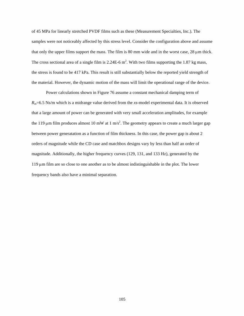
105
of 45 MPa for linearly stretched PVDF films such as these (Measurement Specialties, Inc.). The
samples were not noticeably affected by this stress level. Consider the configuration above and assume
that only the upper films support the mass. The film is 80 mm wide and in the worst case, 28 µm thick.
The cross sectional area of a single film is 2.24E-6 m2. With two films supporting the 1.87 kg mass,
the stress is found to be 417 kPa. This result is still substantially below the reported yield strength of
the material. However, the dynamic motion of the mass will limit the operational range of the device.
Power calculations shown in Figure 76 assume a constant mechanical damping term of
Rm=6.5 Ns/m which is a midrange value derived from the xs-model experimental data. It is observed
that a large amount of power can be generated with very small acceleration amplitudes, for example
the 119 µm film produces almost 10 mW at 1 m/s2. The geometry appears to create a much larger gap
between power generatation as a function of film thickness. In this case, the power gap is about 2
orders of magnitude while the CD case and matchbox designs vary by less than half an order of
magnitude. Additionally, the higher frequency curves (129, 131, and 133 Hz), generated by the
119 µm film are so close to one another as to be almost indistinguishable in the plot. The lower
frequency bands also have a minimal separation.

106
Figure 76 Predicted power vs. acceleration for the 1/2 pint carton device showing performance from a device constructed with two sizes of PVDF film. Results of 62.4, 63.7 and 64.3 Hz are from 28 µm film, the remaining are from 119 µm film.
6.5 Conclusions
This chapter presented a few configurations designed using a fixed volume constraint. The
performance of the designs was estimated using the models created in the previous chapters. As stated
at the beginning, any of the constraints may be used to guide the design including frequency range,
acceleration magnitude, target power, and mass. Additionally, other piezoelectric materials can be
used in place of PVDF by substituting the appropriate materials parameters as shown with the CD case
device where the PVDF films are replace with PZT on brass. Details to the equation variations are
shown in the appendices for the composite materials model.
Predicted power and performance of the different devices showed additional relationships that
must be considered when targeting particular design goals. For example, resonant frequency is often
assumed to be largely a function of mass, however it was shown in the half pint device that the
successful design must also control the stiffness term. Stiffness is shown to be very dependent on the

107
geometry. A comparison of the predicted performance of the devices in this chapter showed the
increase in s with the changes in geometry of the different configurations. This relationship is also
confirmed in Chapter 5, Figure 58 which shows the change in device stiffness with the addition of film
length uxs.

108
CHAPTER SEVEN
7 CONCLUSIONS
This document has presented the need, and one of a number of possible solutions, to the
problem of powering remote devices directly or charging the power storage component of a remote
sensing system. While vibrations may not be the most abundant of harvestable environmental energy,
they certainly have their niche. Extensive research has been conducted on fixed frequency vibration
devices, principally of the cantilever design, that convert the environmental mechanical energy into
electrical energy through electromagnetic and piezoelectric effects. Because of the nature of resonant
frequency oscillators such as cantilevers, which operate most effectively when the vibration of the
device matches the input vibration, considerable design effort must be expended at the front end of an
installation to insure the final design will operate effectively in the intended installation. Researchers
have recognized the limitation of fixed frequency devices and efforts have been expended to move
towards tunable devices.
The XMR device generates energy by stretching a piezoelectric film, and provides a means to
vary the resonant tuning over a wide range through changes in device geometry. Results have shown a
very broad and linear tuning range. A number of prototype devices were constructed with tuning
ranges and details outlined in the Table 12. The initial XMR device shows a tuning range of 86 Hz-
225 Hz. In contrast, tuning ranges in the literature report much lower values. Leland and Wright
demonstrated tuning from 250 Hz to 200 Hz [19], while Challa et al. showed a device with a resonant
frequency of 26 Hz that can tune between 24 Hz and 32 Hz [20]. This requires switching the polarity
of the magnets. The RXMR device has a similar broad adjustment range of 54 Hz-182 Hz. Thicker
films reduces the range from 110 Hz-180 Hz due to the increase in stiffness. Initial modeling
demonstrated a linear power versus acceleration range that was a function of the geometric value up.
As the ratio up/Lo increased, the linear power region with respect to acceleration increased.

109
Table 12 Device performance for various prototype configurations.
Device Mass (g)
Film (µm)
Max Power
Measured (mW)
Frequency Range Tested (Hz)
Working Volume
(cm3)
Acceleration Range Tested (m/s2)
Power/Volume (mW/cm3)
XMR 28.6 28 na 100-225 10 na
XMR 28.6 28 ~0.171 86-154 10 2-10 0.0171 RXMR 65 28 3.2 54-182 21 3-30 0.15 RXMR 82 9 0.3 39-60 21 0.5-4 0.01 RXMR 82 28 12 62-100 21 1-12 0.57 RXMR 82 119 22 110-180 21 0.9-25 1.05
RXMR-xs 82 119 40 332-378 78 0.2-79 0.51 1 Single film operation
Power output for the different configurations is also shown in Table 12. The lowest power
output is from the initial prototype device XMR at ~0.17 mW. The device performance is limited
because of the small area of film and the strain gradients due to the geometry. The RXMR device with
119 µm films made 22 mW and exceeds the 1 mW/cm3 mark initially requested by the Navy. The
power/volume metric allows comparison to other devices in the literature. For example, Perpetuum
sells an fixed frequency commercial harvester using an electromagnetic cantilever design that
produces 4 mW at 100 Hz and 0.04 g acceleration in a 30 cm3 package [60]. This equates to
0.13 mW/cm3. Calculation of an acceleration normalized value results in 3.3 mW/cm3g. The RXMR is
0.42 mW/cm3g. The power output generated by the device was shown to be more strongly affected by
the damping of the device rather than the resonant frequency of operation, which was shown to be
contrary to cantilever devices.
The RXMR (rectangular model) provides additional power output over the original circular
model XMR. This is primarily due to the elimination of strain gradients in the film elements of the
RXMR design. The reduction in the strain gradient allows all the active area of the films to produce
power effectively. Improvements in power are seen by comparing the power/volume metric. Assuming
the single film output would double to 0.034 mW for the XMR device operating with both films, the

110
RXMR produces more than 4 times the power per volume. The reduction in the strain gradient also
prevents premature failure of the films due to plastic deformation.
Modeling developed the relationships for power output based on materials properties and
device geometry. Prototype devices were constructed and evaluated. Results compared favorably to
the model predictions at low acceleration magnitudes. The predictive capabilities for other parameters
such as device stiffness, resonant frequency, coupling, capacitance, optimal load resistance and device
quality factor compare favorably as well. The model can be used as a design tool to optimize a
harvester that can operate through a variety of conditions. Any of the parameters may be used as
design constraints to generate an iterative solution.
Equations were also developed to allow the use of composite material films such as PZT on
brass. The assumption is based on constant strain, i.e. the interface between the composite is ideal. The
ability to use composite films affects a limited number of equations in the model, principally the
capacitance, Co, stiffness, s, and electromechanical coupling term, Ψ.
The modeling was expanded to include additional film lengths, Lxs, to accommodate
geometries that may include piezoceramic structures that are not capable of significant strains but need
to operate in a particular vibration spectrum. At present, the equations of the xs-model tend to over
predict the device stiffness and coupling. Many of the other parameters are determined from these two,
so the error propagates through. However, the power predictions from the model match closely to the
values measured from a prototype device. This may be attributed to the strong dependence in the
power equation on the damping term (which must be measured) and the weak dependence on the
parameters determined from device geometry. The RXMR with excess film shows a reduced tuning
range at a much higher resonant frequency for similar strain ranges, i.e. 332 Hz to 378 Hz. The power
is somewhat lower than the RXMR regular model for similar strains and accelerations as seen in
Figure 64 however the design provides harvesting at accelerations in excess of 75 m/s2.

111
As a design exercise and to show the performance range of the RXMR device a number of
volume limited designs were modeled and evaluated. Frequencies ranged between 3 Hz to 190 Hz and
predicted powers up to 650 mW at 3 m/s2 acceleration. Comparisons are shown for variables such as
film thickness (28 µm and 119 µm) and strains (0.02% to 5.71%) through variation of the pretension
dimension up. In one case, PVDF films are compared with a PZT on brass composite with the
composite PZT structure producing about 120 mW at 3 m/s2 versus 2.5 mW for the PVDF at the same
acceleration. This was accomplished at very low static strain rates of less than 0.0009%. Device
geometry is shown to influence the stiffness of the mechanism which dramatically affects the resonant
frequency. This is particularly evident in the half pint carton device where the mass is very large,
1.8 kgs, however the device geometry drives the stiffness so high that the resonant frequency range
was much higher than anticipated.
There are still many unanswered questions. The performance of PVDF films are known to be
affected by temperature, both high and low. This fact was observed in some experiments conducted in
this research, however the issue has not been addressed in the modeling. PVDF has a very low
piezoelectric coefficient which is why some of the work conducted was on composite PVDF/HFP-
PZT films. There are still many issues to resolve in this system; casting a consistent film, phase
conversion, poling, applying electrodes. The significant difference between some terms in the xs-
model still must be addressed. There is the issue of saturation that is observed in the power output at
higher accelerations and while work has been progressing on this, the solution is not yet at hand.
Other issues would be interesting to pursue, for example, the composite film model could be
expanded to incorporate a bimorph configuration. The single element PVDF films could be doubled or
tripled up, with electrodes in common. Both of these methods would certainly increase the device
stiffness but may also improve power output. Prototype devices could be constructed of PZT on brass
and compared to the predicted results. Additional testing of the xs-model prototype device should be
conducted and used to help clarify the model.

112
This research has provided a design tool that can predict device performance based on
geometry and materials properties. It allows direction in optimizing the power output for a vibration
harvesting device. It has also shown relationships between device parameters and performance.

113
REFERENCES
[1] Beeby, S.P., Torah, R.N., Tudor, M.J., Glynne-Jones, P., Donnell, T.O., Saha, C.R., and Roy, S., A micro electromagnetic generator for vibration energy harvesting. Journal of Micromechanics and Microengineering, 2007(7): p. 1257.
[2] El-hami, M., Glynne-Jones, P., White, N.M., Hill, M., Beeby, S., James, E., Brown, A.D., and Ross, J.N., Design and fabrication of a new vibration-based electromechanical power generator. Sensors and Actuators A: Physical, 2001. 92(1-3): p. 335.
[3] Amirtharajah, R. and Chandrakasan, A.P., Self-powered signal processing using vibration-based power generation. IEEE Journal of Solid-State Circuits, 1998. 33(5): p. 687.
[4] Williams, C.B., Shearwood, C., Harradine, M.A., Mellor, P.H., Birch, T.S., and Yates, R.B., Development of an electromagnetic micro-generator. Circuits, Devices and Systems, IEE Proceedings -, 2001. 148(6): p. 337.
[5] Ching, N.N.H., Li, W.J., Leong, P.H.W., Wen, Z., and Wong, H.Y. A laser-micromachined multi-modal resonating power transducer for wireless sensing systems. 2002. Munich: Elsevier Science B.V.
[6] Roundy, S., Leland, E.S., Baker, J., Carleton, E., Reilly, E., Lai, E., Otis, B., Rabaey, J.M., Wright, P.K., and Sundararajan, V., Improving power output for vibration-based energy scavengers. IEEE Pervasive Computing, 2005. 4(1): p. 28.
[7] Renaud, M., Fiorini, P., and van Hoof, C., Optimization of a piezoelectric unimorph for shock and impact energy harvesting. Smart Materials and Structures, 2007(4): p. 1125.
[8] Stephen, N.G., On energy harvesting from ambient vibration. Journal of Sound and Vibration, 2006. 293(1-2): p. 409.
[9] Beeby, S.P., Tudor, M.J., and White, N.M., Energy harvesting vibration sources for microsystems applications. Measurement Science and Technology, 2006. 17(12): p. 175-195.
[10] Nakano, K., Elliott, S.J., and Rustighi, E., A unified approach to optimal conditions of power harvesting using electromagnetic and piezoelectric transducers. Smart Materials and Structures, 2007. 16(4): p. 948.
[11] Roundy, S., On the effectiveness of vibration-based energy harvesting. Journal of Intelligent Material Systems and Structures, 2005. 16(10): p. 809.
[12] Rossi, G., Marsili, R., Gusella, V., and Gioffre, M., Comparison between accelerometer and laser vibrometer to measure traffic excited vibrations on bridges. Shock and Vibration, 2002. 9(1-2): p. 11.
[13] Lin, C.W. and Yang, Y.B., Use of a passing vehicle to scan the fundamental bridge frequencies: An experimental verification. Engineering Structures, 2005. 27(13): p. 1865.

114
[14] Glanville, M.J., Kwok, K.C.S., and Denoon, R.O., Full-scale damping measurements of structures in Australia. Journal of Wind Engineering and Industrial Aerodynamics, 1996. 59(2-3): p. 349.
[15] Yoshimura, M., Wu, Q., Takahashi, K., Nakamura, S., and Furukawa, K., Vibration analysis of the Second Saikai Bridge--a concrete filled tubular (CFT) arch bridge. Journal of Sound and Vibration, 2006. 290(1-2): p. 388.
[16] Ottman, G.K., Hofmann, H.F., Bhatt, A.C., and Lesieutre, G.A., Adaptive piezoelectric energy harvesting circuit for wireless remote power supply. IEEE Transactions on Power Electronics, 2002. 17(5): p. 669.
[17] Wu, W.J., Chen, Y.F., Chen, Y.Y., Wang, C.S., and Chen, Y.H. Smart wireless sensor network powered by random ambient vibrations. 2007. Taipei, Taiwan: Institute of Electrical and Electronics Engineers Inc., New York, NY 10016-5997, United States.
[18] Roundy, S. and Zhang, Y. Toward self-tuning adaptive vibration based micro-generators. 2005. Sydney, Australia: International Society for Optical Engineering, Bellingham, WA 98227-0010, United States.
[19] Leland, E.S. and Wright, P.K., Resonance tuning of piezoelectric vibration energy scavenging generators using compressive axial preload. Smart Materials and Structures, 2006(5): p. 1413.
[20] Challa, V.R., Prasad, M.G., Shi, Y., and Fisher, F.T., A vibration energy harvesting device with bidirectional resonance frequency tunability. Smart Materials and Structures, 2008(1).
[21] Rastegar, J., Pereira, C., and Nguyen, H.L. Piezoelectric-based power sources for harvesting energy from platforms with low frequency vibration. 2006. San Diego, CA, United States: International Society for Optical Engineering, Bellingham WA, WA 98227-0010, United States.
[22] Shahruz, S.M., Design of mechanical band-pass filters with large frequency bands for energy scavenging. Mechatronics, 2006. 16(9): p. 523.
[23] Tieck, R.M., Carman, G.P., and Enoch Lee, D.G. Electrical energy harvesting using a mechanical rectification approach. 2006. Chicago, IL, United States: American Society of Mechanical Engineers, New York, NY 10016-5990, United States.
[24] Morris, D.J., Youngsman, J.M., Anderson, M.J., and Bahr, D.F., A resonant-frequency tunable, extensional mode piezoelectric vibration harvesting mechanism. Smart Materials and Structures, 2008. 17.
[25] Stachura, S., NTSB investigators surprised by what they found. 2008, Minnesota Public Radio: Minnesota Public Radio Website.
[26] Clegg, W.W., Jenkins, D.F.L., and Cunningham, M.J., The preparation of piezoceramic-polymer thick films and their application as micromechanical actuators. Sensors and Actuators A: Physical, 1997. 58(3): p. 173.
[27] Seema, A., Dayas, K.R., and Varghese, J.M., PVDF-PZT-5H composites prepared by hot press and tape casting techniques. Journal of Applied Polymer Science, 2007. 106(1): p. 146.

115
[28] Naval Research Laboratories Materials Science and Technology Division, Crystal Lattice Structures http://cst-www.nrl.navy.mil/lattice/index.html.
[29] Roundy, S., Wright, P.K., and Rabaey, J., A study of low level vibrations as a power source for wireless sensor nodes. Computer Communications, 2003. 26(11): p. 1131.
[30] Sodano, H.A., Lloyd, J., and Inman, D.J., An experimental comparison between several active composite actuators for power generation. Smart Materials and Structures, 2006. 15(5): p. 1211.
[31] Jeon, Y.B., Sood, R., Jeong, J.H., and Kim, S.G., MEMS power generator with transverse mode thin film PZT. Sensors and Actuators, A: Physical, 2005. 122(1 SPEC ISS): p. 16.
[32] Harrison, J.S. and Ounaies, Z., Piezoelectric Polymers. 2001: Hampton, VA. p. 32.
[33] Linares, A. and Acosta, J.L., Tensile and dynamic mechanical behaviour of polymer blends based on PVDF. European Polymer Journal, 1997. 33(4): p. 467.
[34] Lovinger, A.J., Ferroelectric Polymers. Science, 1983. 220(4602): p. 1115-1121.
[35] El-Hami, K., Ribbe, A., Isoda, S., and Matsushige, K., Structural analysis of the P(VDF/TrFE) copolymer film. Chemical Engineering Science, 2003. 58(2): p. 397.
[36] Chilton, J.A. and Goosey, M.T., eds. Special Polymers for Electronics & Optoelectronics. 1st ed. 1995, Chapman & Hall: London.
[37] Gregorio, R.J., Cestari, M., and Bernardino, F.E., Dielectric behaviour of thin films of β-PVDF/PZT and β- PVDF/BaTiO3 composites. Journal of Materials Science, 1996. 31(11): p. 2925.
[38] Gregorio, R.J. and Cestari, M., Effect of crystallization temperature on the crystalline phase content and morphology of poly(vinylidene fluoride). Journal of Polymer Science, Part B: Polymer Physics, 1994. 32(5): p. 859.
[39] Kepler, R.G., Piezoelectricity, Pyroelectricity, and Ferroelectricity in Organic Materials. Annual Review of Physical Chemistry, 1978. 29(1): p. 497-518.
[40] Thomson, W.T., Theory of vibrations with applications. 2nd ed. 1981, Englewood Cliffs, N.J.: Prentice-Hall, Inc. 493.
[41] Liu, C., Foundations of MEMS. 2006, Upper Saddle River, NJ: Pearson Education, Inc. 530.
[42] Williams, C.B. and Yates, R.B., Analysis of a micro-electric generator for microsystems. Sensors and Actuators, A: Physical, 1996. 52(1-3 pt 1): p. 8.
[43] Zeng, R., Kwok, K.W., Chan, H.L.W., and Choy, C.L., Longitudinal and transverse piezoelectric coefficients of lead zirconate titanate/vinylidene fluoride-trifluoroethylene composites with different polarization states. Journal of Applied Physics, 2002. 92(5): p. 2674.
[44] Socrates, G., Infrared characteristic group frequencies. 1980, Chichester: John Wiley & Sons, Ltd. 153.

116
[45] Lanceros-Mendez, S., Mano, J.F., Costa, A.M., and Schmidt, V.H., FTIR and DSC studies of mechanically deformed β-PVDF films. Journal of Macromolecular Science - Physics, 2001. 40 B(3-4): p. 517.
[46] Goodfellow Corporation, Polyvinylideneflouride (PVDF) Material Information. 2008.
[47] Sullivan, M.S., Development of a novel method for measuring the transverse piezoelectric coefficients of thin piezoelectric films, in Materials Science and Engineering. 2004, Washington State University: Pullman. p. 90.
[48] Robinson, M.C., Microstructural and geometric effects on the piezoelectric perfomance of PZT MEMS, in Materials Science. 2007, Washington State University: Pullman. p. 196.
[49] Anton, S.R. and Sodano, H.A., A review of power harvesting using piezoelectric materials (2003-2006). Smart Materials and Structures, 2007(3): p. R1.
[50] Casciati, F. and Rossi, R., A power harvester for wireless sensing applications. Structural Control & Health Monitoring, 2007. 14(4): p. 649-659.
[51] Mossi, K., Green, C., Ounaies, Z., and Hughes, E., Harvesting energy using a thin unimorph prestressed bender: Geometrical effects. Journal of Intelligent Material Systems and Structures, 2005. 16(3): p. 249.
[52] Kim, H.W., Priya, S., Uchino, K., and Newnham, R.E., Piezoelectric energy harvesting under high pre-stressed cyclic vibrations. Journal of Electroceramics, 2005. 15(1): p. 27.
[53] Cho, J.H., Richards, R.F., Bahr, D.F., Richards, C.D., and Anderson, M.J., Efficiency of energy conversion by piezoelectrics. Applied Physics Letters, 2006. 89(10): p. 104107.
[54] Hu, Y., Xue, H., and Hu, H., A piezoelectric power harvester with adjustable frequency through axial preloads. Smart Materials and Structures, 2007. 16(5): p. 1961.
[55] Mitcheson, P.D., Reilly, E.K., Toh, T., Wright, P.K., and Yeatman, E.M., Performance limits of the three MEMS inertial energy generator transduction types. Journal of Micromechanics and Microengineering, 2007(9): p. S211.
[56] Kino, G., Acoustic waves: devices, imaging, and analog signal processing. 1987, Englewood Cliffs, NJ: Prentice-Hall, Inc. 601.
[57] DuToit, N.E. and Wardle, B.L., Experimental verification of models for microfabricated piezoelectric vibration energy harvesters. AIAA Journal, 2007. 45(5): p. 1126.
[58] Renno, J.M., Daqaq, M.F., and Inman, D.J., On the optimal energy harvesting from a vibration source. Journal of Sound and Vibration, 2009. 320(1-2): p. 386.
[59] Heffernan, R., Precetti, D., and Johnson, W., Vibration Analysis of SA349/2 Helicopter, NASA, Editor. 1991, Publ by NASA: New York, NY, USA. p. 104.
[60] PMG Perpetuum Ltd. http://www.perpetuum.co.uk/.

APPENDIX

118
A1 Materials Properties Information
A1.1 Materials properties of Measurement Specialties, Inc. PVDF

119

120
A1.2 Materials properties for PZT on brass
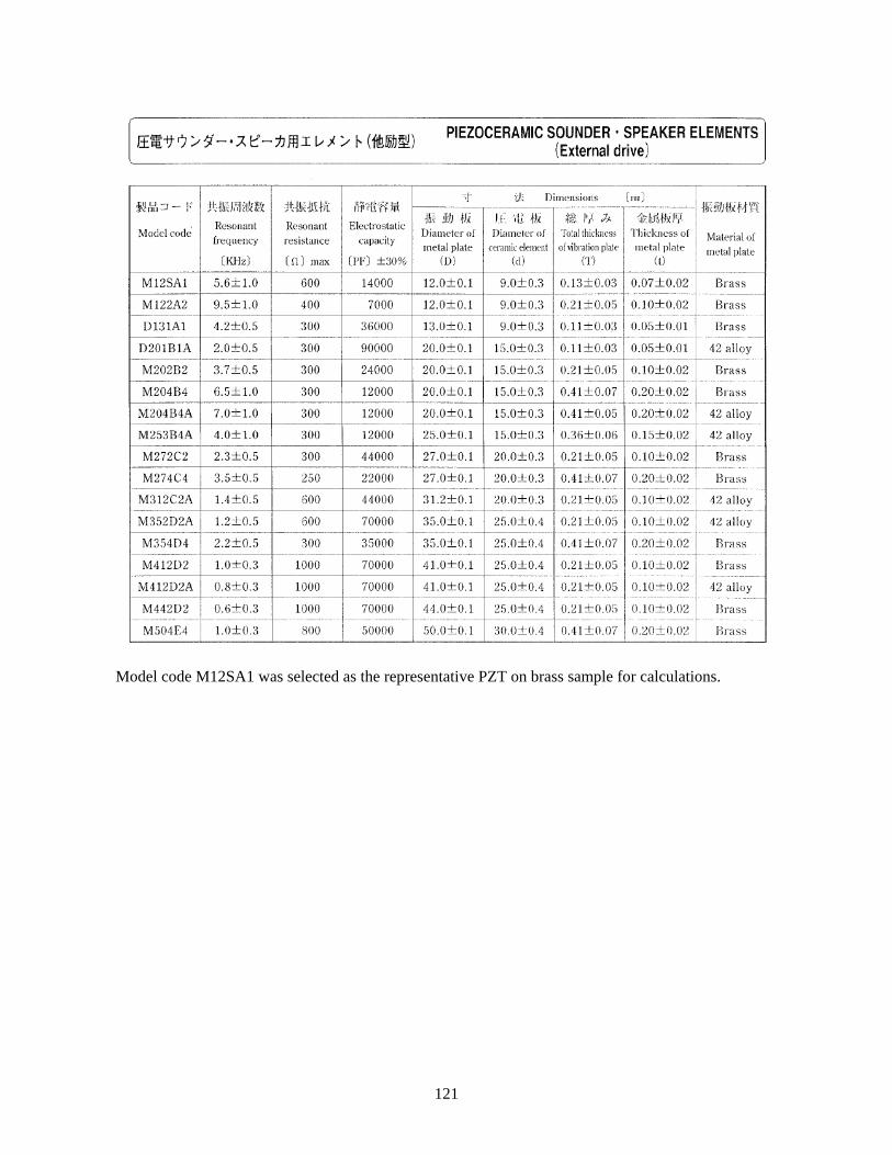
121
Model code M12SA1 was selected as the representative PZT on brass sample for calculations.

122
A2 RXMR Excess Model Development Equations from Mathematica
A2.1 RXMR Tlr App cos a total strain xs.nb

123

124

125

126

127

128

129
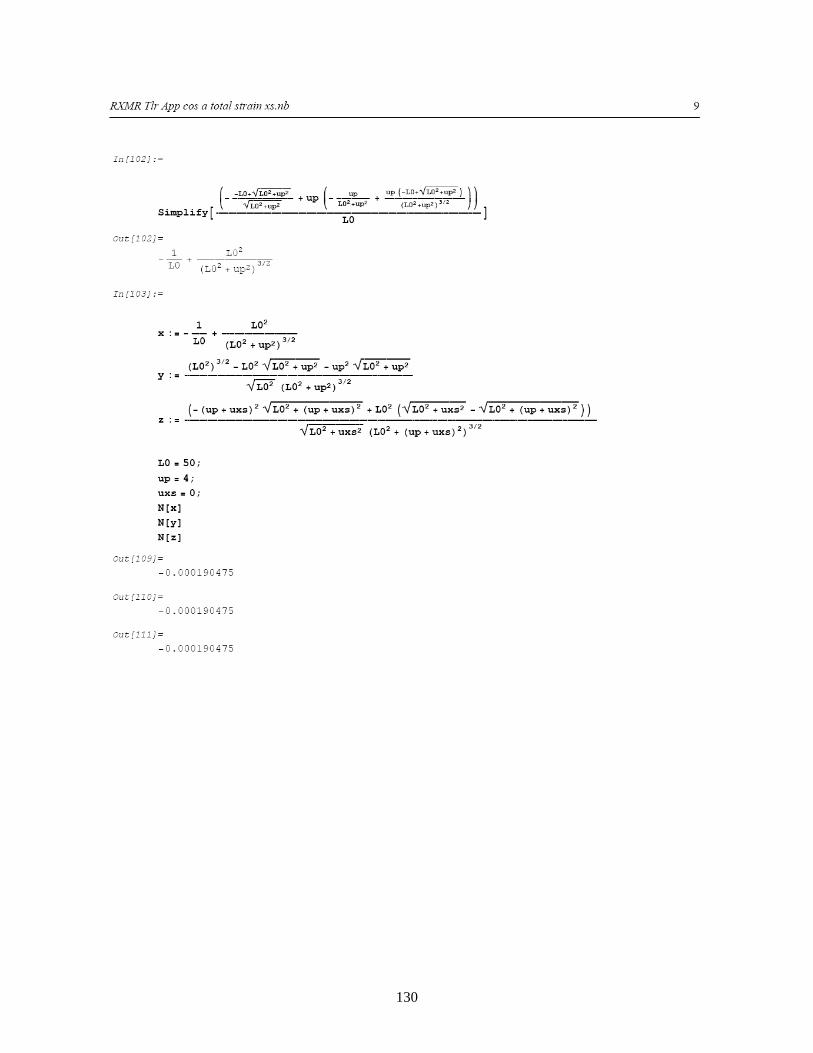
130

131
A2.2 RXMR xs-model power eqn1.nb

132

133

134

135

136

137

138
A2.3 RXMR x- model w dynamic alpha.nb
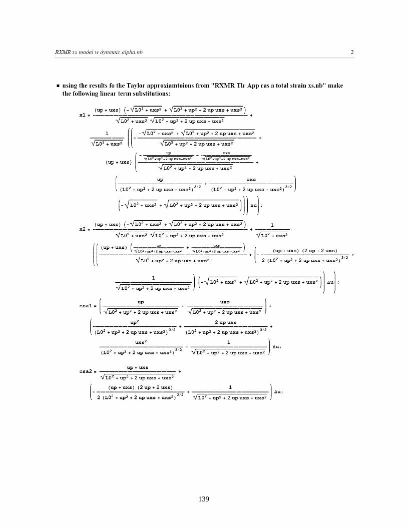
139
140

141

142
A2.4 Variation of wn with up_uxs low freq.nb

143

144

145
A2.5 Variation of wn with up_uxs.nb
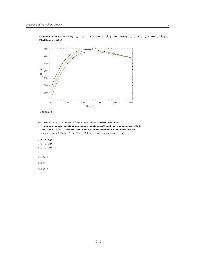
146

147

148
A 2.6 Variation of wn with up_uxs variation of up.nb

149

150

151
A3 Composite Material Thickness Derivation
Derivation for composite substrate: PZT on brass foil for example. Mechanical Portion ha is the thickness of the piezo electric (active) material. hc is the thickness of the composite structure.
11c
Es is the compliance of the composite structure. Starting with
1 31 3 11 1c
ES d E s T= + and
1x
c
NTwh
=
where hc is the thickness of the composite structure. Write the strain equation converting field to voltage realizing that the passive foil layer has d31=0:
1 31 3 31 3 11 10 0 0
c c a c
active passive cc a
h h h hE
h hS dz d E dz d E dz s T dz
−= + +∫ ∫ ∫ ∫
Results in
1 31 11 1c
Ec cS h d V s T h= − +
Using the general form of the derivation from the JSV submission the tension in a film element is
31
11c
cx E
o c
wh L d VNs L h
⎛ ⎞∆= +⎜ ⎟
⎝ ⎠
Using the dynamic Taylor approximation for cosα ∆L/Lo the vertical force for the top and bottom film are written

152
32 2 211 11
0 0
2 211 11
0 0
1 1 11 1
1 1
1 1 11 1
1 1
c c
c c
pc cE E
o op p
pc cE E
o op p
uwh whapproxfortops L s Lu u
L L
uwh whapproxforbottoms L s Lu u
L L
⎛ ⎞⎛ ⎞ ⎜ ⎟⎜ ⎟ ⎜ ⎟⎜ ⎟ ⎜ ⎟= − − −⎜ ⎟ ⎜ ⎟⎜ ⎟ ⎛ ⎞⎛ ⎞ ⎛ ⎞⎜ ⎟+⎜ ⎟ ⎜ ⎟+⎜ ⎟ ⎜ ⎟⎜ ⎟ ⎜ ⎟⎜ ⎟⎝ ⎠⎝ ⎠ ⎝ ⎠⎝ ⎠⎝ ⎠
⎛ ⎞⎜ ⎟⎜ ⎟
= − − − −⎜ ⎟⎜ ⎟⎛ ⎞ ⎛ ⎞+⎜ ⎟ +⎜ ⎟ ⎜ ⎟⎜ ⎟⎝ ⎠⎝ ⎠ ⎝ ⎠
32
⎛ ⎞⎜ ⎟⎜ ⎟⎜ ⎟⎜ ⎟⎛ ⎞⎜ ⎟⎜ ⎟⎜ ⎟⎜ ⎟
⎝ ⎠⎝ ⎠
From the total force equation
2 cos 2 cosT x xF N Nα α+ −= + Write the force equation using the approximations above recognizing that the first term in both approximation equations will cancel:
( )313 22 211 11
1 14 1 2
11c c
pcT U LE E
o o pp
oo
d wuwhF u V Vs L s L uu
LL
⎛ ⎞⎜ ⎟⎜ ⎟⎜ ⎟= − − ∆ − ∆ − ∆⎜ ⎟⎛ ⎞ ⎛ ⎞⎛ ⎞⎜ ⎟ +⎜ ⎟+ ⎜ ⎟⎜ ⎟⎜ ⎟⎜ ⎟ ⎝ ⎠⎝ ⎠⎝ ⎠⎝ ⎠
From this define the coefficients of the terms as:
32 211
14 1
1c
cE
op
o
whss L u
L
⎛ ⎞⎜ ⎟⎜ ⎟⎜ ⎟= −⎜ ⎟⎛ ⎞⎛ ⎞⎜ ⎟⎜ ⎟+ ⎜ ⎟⎜ ⎟⎜ ⎟⎝ ⎠⎝ ⎠⎝ ⎠
and 31
211
12
1c
pE
op
o
d wus L u
L
Ψ =⎛ ⎞
+ ⎜ ⎟⎝ ⎠
Electrical Portion From piezo constitutive equations solve for stress T:

153
1 31 31
11c
E
S d ETs
−=
Sub into D3 equation and write
1 31 33 3 3 31
11
231 1 31 3
3 3 311 11
c
c c
TE
TE E
o
S d ED E ds
d S d ED Es s L
ε
ε
⎛ ⎞−= + ⎜ ⎟⎜ ⎟
⎝ ⎠
= + −
Collecting terms
231 31
3 3 33 11 11
1c c
TT E E
o
d d LD Es s L
εε
⎛ ⎞ ∆= − +⎜ ⎟⎜ ⎟
⎝ ⎠
Convert field to voltage
231 31
3 3 30 0 03 11 11
1a a a
c c
h h hTT E E
o
d L dD dz E dz dzs L s
εε
⎛ ⎞ ∆= − +⎜ ⎟⎜ ⎟
⎝ ⎠∫ ∫ ∫
Limits are of the active piezoelectric material only. This results in
231 31
3 33 11 11
1c c
Ta aT E E
o
d L dD h V hs L s
εε
⎛ ⎞ ∆= − +⎜ ⎟⎜ ⎟
⎝ ⎠
Now integrate over a single electrode
231 31
3 30 0 0 0 0 03 11 11
1o o o
c c
L w L w L wTa aT E E
o
d L dD h dxdy V dxdy h dxdys L s
εε
⎛ ⎞ ∆= − +⎜ ⎟⎜ ⎟
⎝ ⎠∫ ∫ ∫ ∫ ∫ ∫
Which results in the displacement equation written as
231 31
3 33 11 11
1c c
Ta o o o aT E E
o
d L dD h L w L wV L whs L s
εε
⎛ ⎞ ∆= − +⎜ ⎟⎜ ⎟
⎝ ⎠
Substituting the approximation for ∆L/Lo
22 1
p
op
oo
u uLL u
LL
∆∆= −
⎛ ⎞+ ⎜ ⎟
⎝ ⎠
Results in

154
231 31
3 3 23 11 11
2
1
1c c
pTa o o o aT E E
po
o
u ud dD h L w L wV L whs su
LL
εε
⎛ ⎞ ∆= − −⎜ ⎟⎜ ⎟
⎝ ⎠ ⎛ ⎞+ ⎜ ⎟
⎝ ⎠
Now equate wLoD3 to the total free charge attracted to the electrode when connected in series with the lower film, divide through by ha and multiply by 2 for the two elements then:
231 31
3 3 23 11 11
2
2 1 2
1c c
p o aTa o o T E E
po
o
u L whd dD h L w L w V us su
LL
εε
⎛ ⎞= − − ∆⎜ ⎟⎜ ⎟
⎝ ⎠ ⎛ ⎞+ ⎜ ⎟
⎝ ⎠
U UQ C V u− = − ∆ + Ψ∆ Define the coefficients as
23 31
3 11
2 1c
To
T Ea
L w dCh s
εε
⎛ ⎞− = −⎜ ⎟⎜ ⎟
⎝ ⎠
And
312
11
2
1c
pE
po
o
u w dsu
LL
Ψ = −⎛ ⎞
+ ⎜ ⎟⎝ ⎠
Where 2
3 31
3 11
12
c
To
o T Ea
C L w dCh s
εε
⎛ ⎞= = −⎜ ⎟⎜ ⎟
⎝ ⎠

155
A4 Uncertainty Analysis
A4.1 Uncertainty analysis for s and Ψ in the regular model using all terms

156

157

158
A4.2 Uncertainty analysis for s and Ψ in the regular model using all terms except d31

159

160

161
A4.3 Uncertainty analysis for s and Ψ in the regular model using only geometry terms

162

163