SCIENCE CHINA Physics, Mechanics & Astronomy

© Science China Press and Springer-Verlag Berlin Heidelberg 2012 phys.scichina.com www.springerlink.com

*Corresponding author (email: xtianhe@263.net)

• Article • May 2012 Vol.55 No.5: 892–898

doi: 10.1007/s11433-012-4659-z

An improved adaptive Sage filter with applications in GEO orbit determination and GPS kinematic positioning

XU TianHe1,2*, JIANG Nan3 & SUN ZhangZhen3

1 Xi’an Research Institute of Surveying and Mapping, Xi’an 710054, China; 2 GFZ German Research Centre for Geosciences, Potsdam 14473, Germany;

3 College of Geology Engineering and Geomatic, Chang’an University, Xi’an 710054, China

Received August 19, 2011; accepted December 23, 2011; published online February 29, 2012

The shortcomings of an adaptive Sage filter are analyzed in this paper. An improved adaptive Sage filter is developed by using a weighted average quadratic form of the historical residuals of observations and predicted states to evaluate the covariance matrices of observations and dynamic model errors at the present epoch. The weight function is constructed based on the vari-ances of observational residuals or predicted state residuals and the space distance between the previous and the present epoch. In order to balance the contributions of the measurements and the dynamic model information, an adaptive factor is applied by using a two-segment function and predicted state discrepancy statistics. Two applications, orbit determination of a maneuvered GEO satellite and GPS kinematic positioning, are conducted to verify the performance of the proposed method.

Kalman filter, adaptive Sage filter, orbit determination, kinematic positioning, two-segment function

PACS number(s): 91.10.Sp, 93.30.Db, 93.85.Bc, 95.10.Eg

Citation: Xu T H, Jiang N, Sun Z Z. An improved adaptive Sage filter with applications in GEO orbit determination and GPS kinematic positioning. Sci Chi-na-Phys Mech Astron, 2012, 55: 892898, doi: 10.1007/s11433-012-4659-z

The Kalman filter has been widely applied in many fields such as GPS kinematic positioning, GPS/INS integration navigation, satellite orbit determination and so on [1–8]. The performance of a Kalman filter depends on reliable functional and stochastic models. The reliable stochastic models mean that the model errors and their covariance matrices should accurately describe the reliability of dy-namic models and observational information [5,6,9]. In fact, it is very difficult to accurately construct stochastic models using all kinds of prior information. Many kinds of adaptive Kalman filters are developed for evaluating the precision of observations and dynamic models through the posterior information [1,4–6]. One of them is the Sage windowing filter, which is usually applied in kinematic geodetic posi-

tioning and orbit determination [1,5,9,10]. Classical adap-tive stochastic modeling methods can be classified into two groups, namely, innovation-based adaptive modeling and residual-based adaptive modeling. They use the residual (or innovation) vectors of observations and the predicted states from historical epochs to evaluate the covariance matrices of observations and dynamic models errors at the present epoch [5,10]. A moving window-based real time estimation algorithm for a stochastic model of GPS/Doppler navigation is developed by combining the forgetting factor and obser-vation redundancy [11].

Average quadratic forms of the residuals of observations and predicted states within a window are adopted in classi-cal adaptive stochastic modeling, which means that all re-siduals from historical epochs have the same contribution to the evaluation of the covariance matrices of observations and dynamic model errors. In fact, different precision levels

Xu T H, et al. Sci China-Phys Mech Astron May (2012) Vol. 55 No. 5 893

of the historical residuals and the time or space correlation to the present epoch ought to be taken into account. Another problem is that it is hard to precisely describe the dynamic model errors in advance, for example for frequent maneu-vers in GEO satellite orbit maintenance [12–14] and for an aircraft taking off or turning around, which introduces large dynamic model errors into a Kalman filter as well as into a Sage filter. Some kinds of adaptive Sage filters are put for-ward to resist the influence of dynamic model errors [5,9].

In this paper, an improved adaptive Sage filter is devel-oped. It can reasonably evaluate the covariance matrices of the observations and the dynamic model errors at the pre-sent epoch using a weighted average quadratic form of the historical residuals of observations and the predicted states within a window. At the same time, it can efficiently resist the influence of the dynamic model errors by using an adap-tive factor. The structure of this paper is as follows: In sect. 1 a classical Kalman filter and adaptive Sage filter are in-troduced. An improved adaptive Sage filter is developed in sect. 2. Two applications form sect. 3 followed by the con-cluding remarks.

1 Adaptive Sage filter

1.1 Classical Kalman filter

The linearized observation model can be expressed as:

,k k k k= +ΔL A X (1)

where kL is the measurement vector, kA is the design

matrix, kX is the satellite state vector, kΔ is the meas-

urement noise vector, and its covariance matrix is .kΣ

A linear discrete dynamic equation is assumed as:

, 1 1 ,k k k k k = +X Φ X W (2)

where , 1k kΦ is the state transition matrix, kW is the state

noise vector, and its covariance matrix is .k

ΣW

Based on eqs. (1) and (2), the Kalman filter solution can be expressed as:

ˆ ( ),k k k k k X X K L AX (3)

T T 1( ) ,k kk k k k k

= Σ Σ + ΣX XK A A A (4)

ˆ ( ) .kk

k k Σ ΣXXI K A (5)

The predicted state vector and its covariance matrix are

, 1 1ˆ ,k k k k X Φ X (6)

1

Tˆ .

kk kk k

Σ = Σ + ΣWX X

Φ Φ (7)

1.2 Adaptive Sage filter

The covariance matrices of the observations evaluated in an adaptive Sage filter are based on the residual-based adaptive estimation (RAE) or the innovation-based adaptive estima-tion (IAE) [1,10]. In this paper, the REA is analyzed and applied.

The residual vector kV is

ˆ .k k k k V A X L (8)

The corresponding covariance matrices can be derived from eq. (8) as:

Tˆ .

k kk k k Σ Σ ΣV X

A A (9)

If the window width is m, then the covariance matrix of observation vectors based on RAE is

1

T Tˆ

0

1ˆ .k

m

k k j k j k kjm

Σ ΣX

V V A A (10)

In order to avoid using the unknown ˆk

ΣX

at epoch kt in

evaluating ˆ ,kΣ we can use the residual vectors before the

epoch ,kt that is

1

T Tˆ1 1

1

1ˆ .k

m

k k j k j k kjm

Σ ΣX

V V A A (11)

As for adaptive stochastic modeling of dynamic errors, the residual vector of the predicted state vector kΔX is

usually used:

ˆ .k k k ΔX X X (12)

It is easy to obtain the estimate of the matrix of the mod-el errors as in ref. [9],

ˆ .k kk ΔΣ Σ Σ ΣW X XX

(13)

Then the formula for the estimation of the covariance matrix of the dynamic model errors using historical residual vectors of the predicted state at the epoch kt can be ex-

pressed as:

11

Tˆ

1

1ˆ .k kk

m

k j k jjm

Σ Δ Δ Σ ΣW XXX X (14)

2 An improved adaptive Sage filter

From eqs. (11) and (14), it can be seen that adaptive Sage filtering (ASF) uses an average quadratic form of the resid-uals of observations and predicted states within a window to evaluate the covariance matrices of observations and dy-namic model errors at the present epoch. This implies that

894 Xu T H, et al. Sci China-Phys Mech Astron May (2012) Vol. 55 No. 5

all the historical residuals within the window provide the same contribution to the covariance evaluation without con-sidering their differences in precision and correlation in time and space. In order to overcome this problem, a weighted average quadratic form is proposed as:

1

2 T Tˆ1 1

0

ˆ ˆ( ) ,k

m

k k j k j k j k kj

Σ ΣX

V V A A (15)

11

2 Tˆ,

0

ˆ ˆ( , ) ,k k j kk

m

k k j k j k jj

Σ Δ Δ Σ ΣW X XXX X (16)

where 2 2 2, ( ) ( ) ( )k k j k k j k k j k k jx x y y z z is

the geometric distance between the GEO satellite positions ( )k k kx y z at epoch kt and ( )k j k j k jx y z at

epoch .k jt 2ˆk j and 2ˆk j

X are estimates of the vari-

ances of kL and kX at epoch ,k jt respectively. 2ˆ( )k j and 2

, ˆ( , )k jk k j X are the weight functions

related to 2ˆ ,k j 2ˆk j

X and , .k k j The shorter the dis-

tance or the smaller the variance is, the larger the weight is. According to this idea, we construct the weight functions

2ˆ( )k j and 2, ˆ( , )

k jk k j X as:

22 2

1

1 1ˆ( ) ,

ˆ ˆ

m

k jjk j k j

(17)

2, 2 2

1, ,

1 1 1 1ˆ( , ) .

ˆ ˆk j

k j k j

m

k k jjk k j k k j

XX X

(18)

It is easy to construct other forms of the weight function such as the square root or square of the distance , .k k j

Another way is to use interval time to construct the weight function similar to ref. [11]. It is hard to say which one is the best. One may be chosen according to the actual appli-

cation. The approximate formulas for 2ˆk j and 2ˆk j

X can

be written as [9]:

T 1

2ˆ ,k j k j k jk j

k jr

ΣV V

(19)

T 1

2ˆ ,k j

k j

k j k j

k js

Δ Σ ΔX

X

X X (20)

where k jr and k js denote the number of measurements

and the predicted state parameters at ,k jt respectively.

Obviously 2ˆ( )k j and 2, ˆ( , )

k jk k j ΔX satisfy the

following equation:

2 2,

1 1

ˆ ˆ( ) ( , ) 1.k j

m m

k j k k jj j

ΔX (21)

It should be pointed out that using eq. (11) or (15) to es-timate covariance matrices of the observation vectors im-plies that at every epoch the observation information should have the same type, the same distribution and the same di-mension (The observation vectors have the same number of measurements). Otherwise, the covariance matrices of the observation vectors cannot be estimated based on the resid-ual vectors or the innovation vectors.

In order to resist the influence of dynamic model errors, an adaptive Kalman filter is developed [5,9,14,15]. By combining the above adaptive stochastic modeling and the adaptive Kalman filter, the improved adaptive Sage filtering (IASF) estimators follow as [5,9]:

ˆ ( ),k k k k k X X K L AX (22)

1

T T1 1 ˆ ,k kk k k k k

k k

Σ Σ ΣX XK A A A (23)

ˆ ( ) ,kk

k k Σ ΣXXI K A (24)

-1

Tˆ

ˆ ,kk k

k kΣ = Σ + ΣWX XΦ Φ (25)

where k is an adaptive factor and ˆkΣ and ˆ

kΣW are

evaluated by eqs. (15) and (16), respectively. There are three adaptive factors developed in recent

years, which are a three-segment function, a two-segment function and an exponential function [4,14]. Also, three learning statistics, which are a statistic of the predicted state discrepancy, a predicted residual statistic, and a variance component ratio statistic, are constructed to determine the adaptive factor [4,15]. Two optimal adaptive factors are constructed by Yang and Gao [16] to avoid determining the thresh value based on experience. In this paper, the adaptive factor of the two-segment function together with the statistic of the predicted state discrepancy is used [17],

1, ,

, ,

k

kk

k

c

cc

Δ

ΔΔ

X

XX

(26)

where c is a constant, usually c=1.0–2.5. Obviously,

k changes between 0 1.k kΔ X is the statistic of

the predicted state discrepancy, defined as:

,tr( )

k

k k

k

Δ

Σ

X

X XX (27)

where kX is a robust estimate of the state vector [18].

Xu T H, et al. Sci China-Phys Mech Astron May (2012) Vol. 55 No. 5 895

and tr(·) denote the operators of the norm and trace of a ma-trix, respectively. Obviously, if there are dynamic model

errors caused by an orbital maneuver, the value of kΔ X

increases, and k decreases. It should be pointed out that

the position vector is involved in the computation of the

adaptive factor since kX is estimated from the measure-

ments at epoch kt .

The role of eq. (26) is different from that of eq. (16) since the former is to effectively control the influences of dynamic model errors in whole, but the latter is to reasona-bly balance the contribution of historical dynamic infor-mation in windows.

3 Computations and analyses

3.1 Orbit determination for a maneuvered GEO satel-lite

A GEO satellite orbit with an initial longitude of 110.5E degrees and a Chinese ground tracking network consisting of 7 stations over China are simulated. Pseudorange obser-vations for 3 d with 0.3 m white noise and a 30 s sample interval are simulated. Satellite clock bias of 10 m is added to the measurements. The dynamic models include the cen-tral gravity of the earth, the gravity field model JGM-3 up to degree and order of 8, the lunar, solar and other planets’ gravitational effect, a spherical solar radiation pressure model and a thrust force model with a constant impulse in the direction of the velocity. Every day a simulated maneu-ver of 30 min is performed at 12 o’clock. The constant im-pulse burn accelerations of the three maneuvers are 6×105, 7×105 and 8×105 m/s2 along the velocity direction, re-spectively. The corresponding thrust force model is as fol-lows [13]:

burn burn ,x

y

z

v

v

v

e

a e

e

a

where burna is the thrust force vector, burna is the con-

stant impulse burn acceleration, and ( )x y z

e e e v v v

x y zv v vv v v is the unit vector of the velocity.

The resolved parameters are the six state parameters of position and velocity as well as a solar radiation coefficient and a satellite clock bias. Initial parameter errors for the position, velocity, clock bias and radiation pressure coeffi-cient are 5 m, 5 m, 5 m, 0.5 m/s, 0.5 m/s, 0.5 m/s, 5 m and 0.1, and their initial variances are 104 m2, 104 m2 , 104 m2, 10 (m/s)2, 10 (m/s)2, 10 (m/s)2, 10 m2 and 1, respectively. The covariance matrix of the process noise is assumed as

kΣW =

diag[(0.01 m)2, (0.01 m)2, (0.01 m)2, (0.0001 m/s)2, (0.0001 m/s)2, (0.0001 m/s)2, (1 m)2, (0.01)2]. The window width m in eqs. (15)–(18) and the constant c in eq. (26) are chosen as 10 and 2.0, respectively, according to experience. The computations for the following seven schemes are per-formed and compared.

Scheme 1 ASF without thrust force. Scheme 2 IASF without thrust force. Scheme 3 IASF only using eq. (16) without thrust

force. Scheme 4 The same as Scheme 2 but using the root of

the distance to construct the weight function. Scheme 5 The same as Scheme 2 but using the square

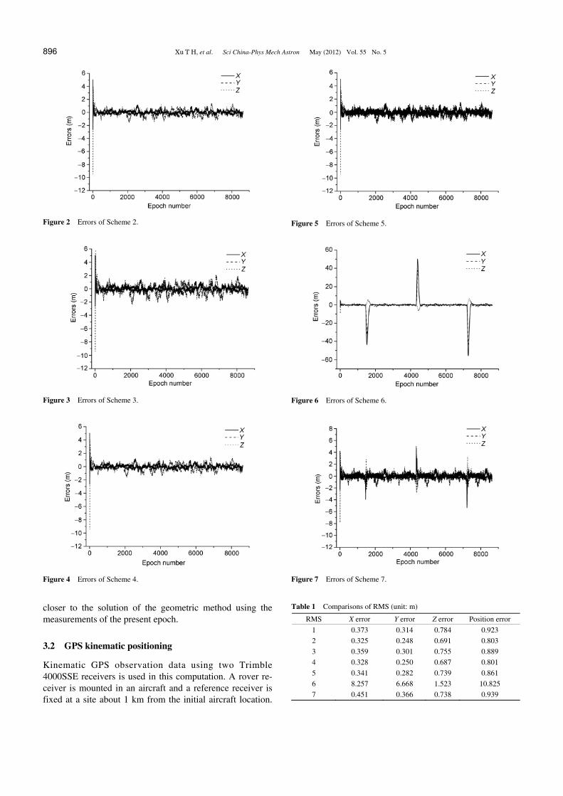
of the distance to construct the weight. Scheme 6 ASF with thrust force. Scheme 7 IASF with thrust force. The errors in the directions of the 3 axes X, Y and Z are

given in Figures 1–7. The RMS comparisons are displayed in Table 1.

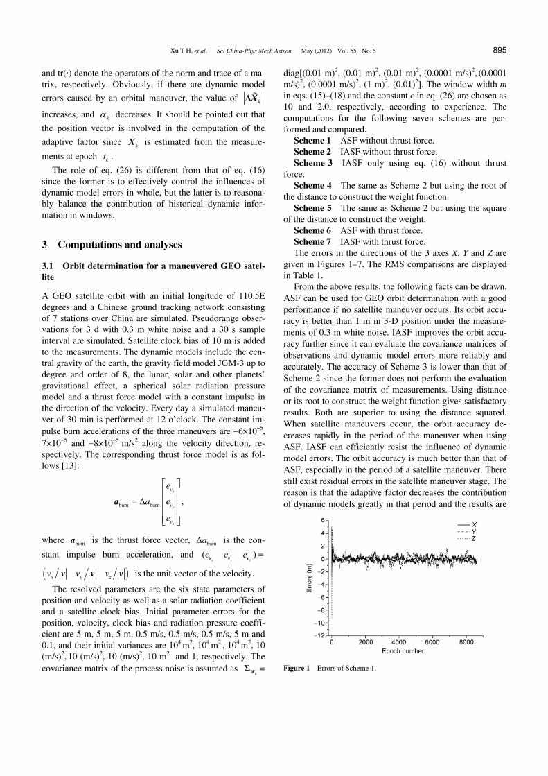
From the above results, the following facts can be drawn. ASF can be used for GEO orbit determination with a good performance if no satellite maneuver occurs. Its orbit accu-racy is better than 1 m in 3-D position under the measure-ments of 0.3 m white noise. IASF improves the orbit accu-racy further since it can evaluate the covariance matrices of observations and dynamic model errors more reliably and accurately. The accuracy of Scheme 3 is lower than that of Scheme 2 since the former does not perform the evaluation of the covariance matrix of measurements. Using distance or its root to construct the weight function gives satisfactory results. Both are superior to using the distance squared. When satellite maneuvers occur, the orbit accuracy de-creases rapidly in the period of the maneuver when using ASF. IASF can efficiently resist the influence of dynamic model errors. The orbit accuracy is much better than that of ASF, especially in the period of a satellite maneuver. There still exist residual errors in the satellite maneuver stage. The reason is that the adaptive factor decreases the contribution of dynamic models greatly in that period and the results are

Figure 1 Errors of Scheme 1.

896 Xu T H, et al. Sci China-Phys Mech Astron May (2012) Vol. 55 No. 5

Figure 2 Errors of Scheme 2.

Figure 3 Errors of Scheme 3.

Figure 4 Errors of Scheme 4.

closer to the solution of the geometric method using the measurements of the present epoch.

3.2 GPS kinematic positioning

Kinematic GPS observation data using two Trimble 4000SSE receivers is used in this computation. A rover re-ceiver is mounted in an aircraft and a reference receiver is fixed at a site about 1 km from the initial aircraft location.

Figure 5 Errors of Scheme 5.

Figure 6 Errors of Scheme 6.

Figure 7 Errors of Scheme 7.

Table 1 Comparisons of RMS (unit: m)

RMS X error Y error Z error Position error

1 0.373 0.314 0.784 0.923

2 0.325 0.248 0.691 0.803

3 0.359 0.301 0.755 0.889

4 0.328 0.250 0.687 0.801

5 0.341 0.282 0.739 0.861

6 8.257 6.668 1.523 10.825

7 0.451 0.366 0.738 0.939

Xu T H, et al. Sci China-Phys Mech Astron May (2012) Vol. 55 No. 5 897

After about 10 min of static tracking, the aircraft takes off for a flight time of about 90 min. The measurements used are P code, L1 and L2 carrier phases with a second data rate. In order to analyze the influences of the vehicle dis-turbances on various filtering results, the highly precise results from double-differenced carrier phase measurements are used as reference values to compare with the results from the code measurements. The constant velocity model is employed and the initial variances for the positions, ve-locities, and P2-code measurements are selected as 0.2 m2, 9×106 m2·s2, and 1 m2 separately. The velocities spectral density is chosen as 0.2 m2·s2. The dynamic model covari-ance matrix is chosen as [17]:

3 22 2

22 2

1 1

3 2 .1

2

t

Q t Q t

Q t Q t

W

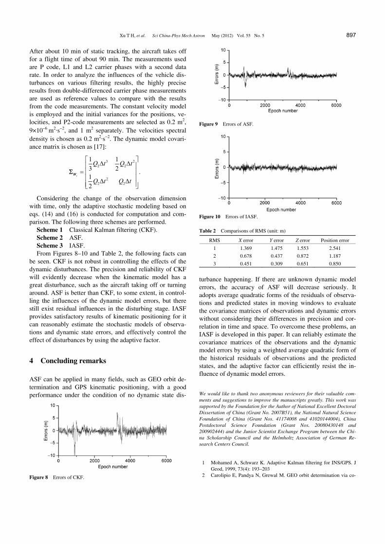
Considering the change of the observation dimension with time, only the adaptive stochastic modeling based on eqs. (14) and (16) is conducted for computation and com-parison. The following three schemes are performed.

Scheme 1 Classical Kalman filtering (CKF). Scheme 2 ASF. Scheme 3 IASF. From Figures 8–10 and Table 2, the following facts can

be seen. CKF is not robust in controlling the effects of the dynamic disturbances. The precision and reliability of CKF will evidently decrease when the kinematic model has a great disturbance, such as the aircraft taking off or turning around. ASF is better than CKF, to some extent, in control-ling the influences of the dynamic model errors, but there still exist residual influences in the disturbing stage. IASF provides satisfactory results of kinematic positioning for it can reasonably estimate the stochastic models of observa-tions and dynamic state errors, and effectively control the effect of disturbances by using the adaptive factor.

4 Concluding remarks

ASF can be applied in many fields, such as GEO orbit de-termination and GPS kinematic positioning, with a good performance under the condition of no dynamic state dis-

Figure 8 Errors of CKF.

Figure 9 Errors of ASF.

Figure 10 Errors of IASF.

Table 2 Comparisons of RMS (unit: m)

RMS X error Y error Z error Position error

1 1.369 1.475 1.553 2.541

2 0.678 0.437 0.872 1.187

3 0.451 0.309 0.651 0.850

turbance happening. If there are unknown dynamic model errors, the accuracy of ASF will decrease seriously. It adopts average quadratic forms of the residuals of observa-tions and predicted states in moving windows to evaluate the covariance matrices of observations and dynamic errors without considering their differences in precision and cor-relation in time and space. To overcome these problems, an IASF is developed in this paper. It can reliably estimate the covariance matrices of the observations and the dynamic model errors by using a weighted average quadratic form of the historical residuals of observations and the predicted states, and the adaptive factor can efficiently resist the in-fluence of dynamic model errors.

We would like to thank two anonymous reviewers for their valuable com-ments and suggestions to improve the manuscripts greatly. This work was supported by the Foundation for the Author of National Excellent Doctoral Dissertation of China (Grant No. 2007B51), the National Natural Science Foundation of China (Grant Nos. 41174008 and 41020144004), China Postdoctoral Science Foundation (Grant Nos. 20080430148 and 200902444) and the Junior Scientist Exchange Program between the Chi-na Scholarship Council and the Helmholtz Association of German Re-search Centers Council.

1 Mohamed A, Schwarz K. Adaptive Kalman filtering for INS/GPS. J Geod, 1999, 73(4): 193–203

2 Carolipio E, Pandya N, Grewal M. GEO orbit determination via co-

898 Xu T H, et al. Sci China-Phys Mech Astron May (2012) Vol. 55 No. 5

variance analysis with a known clock error. Navigation, 2001, 48(4): 255–260

3 Grewal M, Carolipio E, Bailey M. Comparison of GEO and GPS or-bit determination. In: ION GPS 2002. Portland: Oregon Convention Center, 2002. 790–799

4 Yang Y X, He H B, Xu G C. Adaptively robust filtering for kinemat-ic geodetic positioning. J Geod, 2001, 75(2): 109–116

5 Yang Y X, Wen Y L. Synthetically adaptive robust filtering for satel-lite orbit determination. Sci China Ser D-Earth Sci, 2004, 47(7): 585–592

6 Ding W D, Wang J L, Rizos C. Improving adaptive Kalman estima-tion in GPS/INS integration. J Navig, 2007, 60(4): 517–529

7 He K F, Xu T H. Kinematic orbit determination of GEO satellite based on Kalman filtering. J Geod Geodyn, 2009, 29(6): 109–114

8 Almagbile A, Wang J L, Ding W D. Evaluating the performances of adaptive Kalman filter methods in GPS/INS integration. J Global Posit Syst, 2010, 9(1): 33–40

9 Yang Y X, Xu T H. An adaptive Kalman filter based on Sage win-dowing weights and variance components. J Navig, 2003, 56(2): 231–240

10 Sage A, Husa G. Adaptive filtering with unknown prior statistics. In: Proceedings of the Joint American Control Conference. Boulder Col-

orado, US, 1969. 760–769 11 Zhou Z B, Shen Y Z, Li B F. Moving time-window based real-time

estimation algorithm for the stochastic model of GPS/Doppler navi-gation. Acta Geod Et Cartogr Sin, 2011, 40(2): 220–225

12 Su H. Precise Orbit Determination of Global Navigation Satellite System of Second Generation (GNSS-2)-Orbit Determination of IGSO, GEO and MEO Satellites. Dissertation for Doctoral Degree. Munich: University of Bundswehr, 2000

13 Montenbruck O, Gill E. Satellite Orbits: Models, Methods and Ap-plications. Heidelberg: Springer, 2000

14 Huang Y, Hu X G, Huang C, et al. Precise orbit determination of a maneuvered GEO satellite using CAPS ranging data. Sci China Ser G-Phys Mech Astron, 2009, 52(6): 346–352

15 Yang Y X, Gao W G. Influence comparison of adaptive factors on navigation results. J Navig, 2005, 58(3): 471–478

16 Yang Y X, Gao W G. An optimal adaptive Kalman filter. J Geod, 2006, 80(3): 177–183

17 Yang Y X, Gao W G. A new learning statistic for adaptive filter based on predicted residuals. Prog Nat Sci, 2006, 16(8): 833–837

18 Yang Y X. Robust estimator for dependent observations. Manuscr Geod, 1994, 19: 10–17