an improved weighted essentially non-oscillatory scheme with a new smoothness indicator

Journal of Computational Physics 232 (2013) 68–86

Contents lists available at SciVerse ScienceDirect

Journal of Computational Physics

journal homepage: www.elsevier .com/locate / jcp

An improved weighted essentially non-oscillatory scheme with a newsmoothness indicator

Youngsoo Ha a, Chang Ho Kim b, Yeon Ju Lee c, Jungho Yoon d,⇑a National Institute for Mathematical Sciences, Daejeon 305-811, Republic of Koreab Department of Computer Engineering, Glocal Campus, Konkuk University, 380-701 Chungju, Republic of Koreac Institute of Mathematical Sciences, Ewha W. University, Seoul 120-750, Republic of Koread Department of Mathematics, Ewha W. University, Seoul 120-750, Republic of Korea

a r t i c l e i n f o

Article history:Received 2 September 2011Received in revised form 23 April 2012Accepted 11 June 2012Available online 27 June 2012

Keywords:Hyperbolic conservation lawsEuler equationWENO schemeApproximation orderSmoothness indicator

0021-9991/$ - see front matter � 2012 Elsevier Inchttp://dx.doi.org/10.1016/j.jcp.2012.06.016

⇑ Corresponding author.E-mail addresses: [email protected] (Y. Ha),

a b s t r a c t

In this paper, we present a new smoothness indicator that evaluates the local smoothnessof a function inside of a stencil. The corresponding weighted essentially non-oscillatory(WENO) finite difference scheme can provide the fifth convergence order in smoothregions, especially at critical points where the first derivative vanishes (but the secondderivatives are non-zero). We provide a detailed analysis to verify the fifth-order accuracy.Some numerical experiments are presented to demonstrate the performance of the pro-posed scheme. We see that the proposed WENO scheme provides at least the same orimproved behavior over the fifth-order WENO-JS scheme [10] and other fifth-order WENOschemes called as WENO-M [9] and WENO-Z [2], but its advantage seems more salient intwo dimensional problems.

� 2012 Elsevier Inc. All rights reserved.

1. Introduction

The goal of this paper is to introduce an improved version of the fifth-order WENO finite difference scheme for theapproximation of hyperbolic conservation laws in the form

qt þ f ðqÞx ¼ 0; x 2 R; t P 0;qðx;0Þ ¼ q0ðxÞ;

ð1:1Þ

with proper boundary conditions. Here, the function q ¼ ðq1; . . . ; qmÞ is an m-dimensional vector of conserved quantities andthe flux f ðqÞ is a vector-valued function of m components. Eq. (1.1) is called hyperbolic if all eigenvalues fkkðqÞg of the Jaco-bian matrix

A ¼ @f@q;

of the flux function are real and the set of right eigenvectors is complete.Since the (exact) solution of the hyperbolic Eq. (1.1) may develop discontinuities—shock and contact—in finite time, one

needs shock-capturing schemes without creating spurious oscillations. Among many numerical schemes for solving (1.1),ENO (essentially non-oscillatory) [7,8,16,17] and Weight ENO (WENO) schemes [10,12] have been quite successful in appli-cations with shocks, contact discontinuities, and complicated smooth solutions. The ENO scheme, which is a modification of

. All rights reserved.

[email protected] (C. Kim), [email protected] (Y. Lee), [email protected] (J. Yoon).

http://dx.doi.org/10.1016/j.jcp.2012.06.016

mailto:[email protected]




http://dx.doi.org/10.1016/j.jcp.2012.06.016

http://www.sciencedirect.com/science/journal/00219991

http://www.elsevier.com/locate/jcp

Y. Ha et al. / Journal of Computational Physics 232 (2013) 68–86 69

the total variation diminishing (TVD) scheme [5], is designed to use an adaptive stencil based on the local smoothness suchthat it yields high-order accuracy where the function is smooth but avoids the Gibbs phenomena at discontinuities. To dothis, a smoothness indicator of a solution is first determined over each stencil and then, by using this, the smoothest oneis chosen from a set of candidate stencils. As a result, an ENO scheme obtains information from smooth regions and avoidsspurious oscillations near discontinuities. The cell-average version of ENO schemes has the disadvantage of complicatetransfers between point values and cell averages for a higher order accuracy in multi-spatial dimension problems. To elim-inate these complications, efficient ENO schemes based on point values rather than cell averages were introduced by Shu andOsher [16,17]. Also, Serna and Marquina [14] introduced power ENO methods using an extended class of limiters to classicalENO schemes to improve the algorithmic behavior near discontinuities.

The WENO scheme, an improved version of the ENO technique using a cell-averaged approach, was introduced by Liu,Osher, and Chan [12]. It uses a nonlinear convex combination of all the candidate stencils to improve the accuracy of numericalfluxes without destroying non-oscillatory behaviors near discontinuities. This process is performed by weighting the contri-bution of the local flux according to its smoothness on each stencil such that the weight of the solution on a stencil containing adiscontinuity is essentially zero. In doing this, the corresponding WENO scheme can achieve a high order accuracy withoutoscillations near discontinuities or sharp gradient regions. Specifically, the roles of smoothness indicators in WENO schemesare (1) improving the convergence order at the smooth regions, (2) decreasing the dissipation near discontinuities, and (3)maintaining the stability without destroying the essentially non-oscillatory behavior. In the paper [10], Jiang and Shu intro-duced a smoothness indicator, which is the sum of the normalized squares of the scaled L2�norms of the all derivatives of thelower order polynomials, and extended a finite difference (flux) version of WENO schemes [12] to third- and fifth-order accu-rate methods (hereafter, denoted by WENO-JS). However, Henrick, Aslam, and Powers pointed out that the actual convergencerate of the fifth-order WENO-JS in [10] is less than fifth order for many problems [9]. They demonstrated that the smoothnessindicator of WENO-JS was failed to recover the maximum order of the scheme at critical points where the third order deriv-atives do not simultaneously vanish with the first. In the same article, they introduced a new fifth-order WENO method (calledWENO-M) fixing this problem by modifying the smoothness indicator of WENO-JS to satisfy sufficient criteria for fifth-orderconvergence. They devised a correcting mapping and applied it to the smoothness indicator of WENO-JS. Compared to theWENO-JS scheme, the WENO-M scheme can achieve the optimal convergence order at critical points of smooth parts, reducethe numerical dissipation, and obtain sharper results near discontinuities. In [2], Borges, Carmona, Costa, and Don introducedanother version of the fifth-order WENO scheme (called WENO-Z) with a new smoothness indicator which is constructed byincorporating a global higher order smoothness measurement into the weights of the WENO-JS scheme. This method allows usto obtain the optimal convergence order at the critical points of smooth regions of the solution and captures shock in a phys-ically sharp manner with maintaining stability and the essentially non-oscillatory behavior. The WENO-Z scheme has thesame accuracy as the WENO-M scheme but generates improved results. Higher order WENO schemes also have been devel-oped. Balsara and Shu [1] introduced WENO methods up to the eleventh order. In [4], Gerolymos, Sénéchal, and Vallet ex-tended both the WENO-JS and WENO-M schemes up to the seventeenth order. In addition, Castro, Costa, and Don provideda closed-form formula for higher than fifth order smoothness indicators of the WENO-Z scheme in [3].

In this article, we derive a new method that measures the (local) smoothness of the numerical solution inside a stencil.The associated WENO scheme (hereafter, denoted by WENO-NS) can get the fifth convergence order in smooth regions, evenat critical points where the first derivative vanishes (but the secod derivatives are non-zero). For the construction of the newsmoothness indicator, we first introduce a generalized version of undivided difference that approximates the derivatives ofthe flux functions more accurately. Based on this approximation, a new smoothness indicator is constructed. An interestingfeature is that there is a parameter that governs the tradeoff between the accuracies around the smooth region and discon-tinuous region. A good choice for the parameters can be interpreted as a balanced compromise between smoothness anddiscontinuity of the data. Some numerical experiments are presented to demonstrate the performance of the proposedscheme. The WENO-NS scheme provides at least similar or improved behavior over other fifth-order WENO schemes:WENO-JS, WENO-M and WENO-Z. Also, we will see that the advantage of the proposed scheme seems more salient intwo dimensional problems.

The rest of this paper is organized as follows. Section 2 provides a brief review of the WENO schemes for one-dimensionalscalar conservation laws. In Section 3, we provide a new smoothness indicator and the associated fifth-order WENO scheme.Section 4 presents some numerical results to demonstrate the ability of the proposed WENO scheme, and a conclusion ispresented in Section 5.

2. Review of the WENO schemes

In this section, we briefly describe the fifth-order WENO finite difference scheme for one-dimensional scalar conservationlaws. Let fIjg be a partition of a given domain with the jth cell Ij :¼ ½xj�1=2; xjþ1=2�. The center of Ij is denoted byxj ¼ 1

2 ðxj�1=2 þ xjþ1=2Þ and the value of a function f at the location xj is denoted by using the subscript j, i.e., fj ¼ f ðxjÞ. In whatfollows, for practical use, we assume that the set fxjþ1=2gj is uniformly gridded. Then, the notation Dx ¼ xjþ1=2 � xj�1=2 indi-cates the size of Ij.

The one-dimensional hyperbolic conservation laws in (1.1) can be approximated by a system of ordinary differentialequations, where the spatial derivative has been replaced by a finite difference, so that it yields the semi-discrete form:

70 Y. Ha et al. / Journal of Computational Physics 232 (2013) 68–86

dqj

dt¼ � 1

Dxðf̂ jþ1=2 � f̂ j�1=2Þ; ð2:1Þ

where qjðtÞ is the numerical approximation to the point value qðxj; tÞ in a grid and f̂ j�1=2 are numerical fluxes.The numerical flux f̂ has to satisfy a Lipschitz continuity in each of its arguments and is consistent with the physical flux f,

that is, f̂ ðq; . . . ; qÞ ¼ f ðqÞ. To compute the numerical flux f̂ j�1=2, we define a function h implicitly through the following equa-tion (see Lemma 2.1 of [17]),

f ðqðxÞÞ ¼ 1Dx

Z xþDx=2

x�Dx=2hðnÞdn: ð2:2Þ

Differentiating (2.2) with respect to x leads to

f ðqðxÞÞx ¼1Dx

h xþ Dx2

� �� h x� Dx

2

� �� ; ð2:3Þ

which indicates that the numerical flux f̂ j�1=2 should approximate hðxj�1=2Þ to a high order, that is, f̂ j�1=2 ¼ hðxj�1=2Þ þ OðDx5Þ.Practically, to avoid entropy violating solutions and ensure the numerical stability, the flux f ðqÞ is splitted into two compo-nents fþ and f� so that

f ðqÞ ¼ fþðqÞ þ f�ðqÞ; ð2:4Þ

where dfþðqÞdq P 0 and df�ðqÞ

dq 6 0. One of the simplest flux splittings is the Lax–Friedrichs splitting which is given by

f�ðqÞ ¼ 12ðf ðqÞ � aqÞ; ð2:5Þ

where a ¼maxqjf 0ðqÞj over the pertinent range of q. Then the WENO scheme is apply to f�ðqÞ ¼ 12 ðf ðqÞ � aqÞ to obtain the

numerical flux. Let f̂þjþ1=2 and f̂�jþ1=2 be the numerical fluxes at x ¼ xjþ1=2 obtained from (2.2) for the positive and negative partsof f ðqÞ respectively, and let

f̂ jþ1=2 ¼ f̂þjþ1=2 þ f̂�jþ1=2: ð2:6Þ

Hereafter, we will only describe how f̂þjþ1=2 is approximated for (2.3) because the formulas for the negative part of the splitflux (2.6) are symmetric to the positive part with respect to xjþ1=2, Also, for simplicity, we will drop the ‘+’ sign in thesuperscript.

2.1. Fifth-order WENO

In order to construct f̂ jþ1=2, the classical fifth-order WENO scheme uses a 5-point stencil which is subdivided intothree candidate substencils. A numerical flux is calculated for each stencil and the local solutions are then averagedin a way of retaining the fifth-order convergence in smooth regions. However, in order to better approximate derivativesnear shocks, the weights should effectively remove the contribution of stencils which contain the discontinuity. To bemore precise, let

SkðjÞ :¼ fxjþk�2; xjþk�1; xjþkg; k ¼ 0;1;2 ð2:7Þ

be the stencil consisting of 3-points starting at xjþk�2, and let

f̂ kjþ1=2 ¼

X2

‘¼0

ck;‘fjþk�2þ‘ ð2:8Þ

be the second degree polynomial approximation constructed on the stencil SkðjÞ to approximate the value hðxjþ1=2Þwhere ck;‘

(‘ ¼ 0;1;2) are the Lagrange interpolation coefficients depending on the left-shift parameter k. The specific expression off̂ k

jþ1=2 can be written as

f̂ 0jþ1=2 ¼

16

2f j�2 � 7f j�1 þ 11f j

� �;

f̂ 1jþ1=2 ¼

16�fj�1 þ 5f j þ 2f jþ1

� �;

f̂ 2jþ1=2 ¼

16

2f j þ 5f jþ1 � fjþ2� �

:

ð2:9Þ

To define f̂ kj�1=2, each index needs to be shifted by �1. Moreover, by using the Taylor expansions of the equations in (2.9), we

can get the expression


f̂ 0j�1=2 ¼ hj�1=2 �

14

f 000ð0ÞDx3 þ OðDx4Þ;

f̂ 1j�1=2 ¼ hj�1=2 þ

112

f 000ð0ÞDx3 þ OðDx4Þ;

f̂ 2j�1=2 ¼ hj�1=2 �

112

f 000ð0ÞDx3 þ OðDx4Þ:

ð2:10Þ

Then these functions are combined to define a new WENO approximation to the value hðxjþ1=2Þ, that is,

f̂ jþ1=2 ¼X2

k¼0

xkf̂ kjþ1=2: ð2:11Þ

To construct the weights xk, let us consider the case that the function h is smooth on all the stencils SkðjÞwith k ¼ 0;1;2. Then,we first find the constants dk such that its linear combination with f̂ k

jþ1=2 retains the fifth convergence order to hðxjþ1=2Þ, that is,

hðxjþ1=2Þ ¼X2

k¼0

dkf̂ kjþ1=2 þOðDx5Þ:

The coefficients dk are called the ideal weights since they generate the central upstream fifth-order scheme for the 5-pointstencil. The specific values of dk are as follows (e.g., see [15]):

d0 ¼ 1=10; d1 ¼ 3=5; d2 ¼ 3=10: ð2:12Þ

Using these numbers dk, the nonlinear weights xk are defined by

xk ¼akX2

‘¼0

a‘

and ak ¼dk

ðeþ bkÞ2 ; ð2:13Þ

where 0 < e� 1 is introduced to prevent the denominator becoming zero, and where bk is a smoothness indicator of the fluxf̂ k. Now, recall that each of f̂ k

jþ1=2 takes the form

f̂ kj�1=2 ¼ hj�1=2 þ AkDx3 þ OðDx4Þ; k ¼ 0;1;2;

where the specific form of Ak has been given in (2.10). Then, it is well-known (e.g., see [2,9]) that necessary and sufficientconditions for the fifth-order convergence in (2.3) are given by

X2

k¼0

ðx�k � dkÞ ¼ OðDx6Þ;

X2

k¼0

Akðxþk �x�k Þ ¼ OðDx3Þ;

x�k � dk ¼ OðDx2Þ;

ð2:14Þ

where superscripts ‘þ’ and ‘�’ on xk correspond to their use in either f kjþ1=2 and f k

j�1=2 stencils respectively. Since the firstequation in (2.14) holds always due to the normalization, a sufficient condition for the fifth-order convergence is

x�k � dk ¼ OðDx3Þ: ð2:15Þ

2.2. The WENO-JS scheme

The smoothness indicator bk suggested by Jiang and Shu [10] is given by

bk ¼X2

‘¼1

Z xjþ1=2

xj�1=2

Dx2‘�1 d‘

dx‘f̂ k

!2

dx: ð2:16Þ

These indicators take on an explicit form:

b0 ¼14ðfj�2 � 4f j�1 þ 3f jÞ

2 þ 1312ðfj�2 � 2f j�1 þ fjÞ2;

b1 ¼14ðfj�1 � fjþ1Þ2 þ

1312ðfj�1 � 2f j þ fjþ1Þ2;

b2 ¼14ð3f j � 4f jþ1 þ fjþ2Þ2 þ

1312ðfj � 2f jþ1 þ fjþ2Þ2:

ð2:17Þ

We remark that this indicator is similar to, but smoother than, the total variation measurement based on the L1 norm. It isobvious that bk in (2.16) satisfies the condition


bk ¼ Dð1þOðDx2ÞÞ; ð2:18Þ

where the constant D is independent of k but may depend on Dx [15]. It implies that the WENO weights xk (k ¼ 0;1;2) sat-isfy the condition

dk �xk ¼ OðDx2Þ: ð2:19Þ

This requires the second equation of (2.14) should be satisfied; but it can be confirmed by a symbolic computation. Then thefinal WENO construction provides the fifth convergence order in the smooth region [15]. However, at critical point where thefirst derivative of f vanishes, bk is of the form bk ¼ Dð1þ OðDxÞÞ, yielding xk ¼ dk þ OðDxÞ. It results in the loss of convergenceorder of the scheme to the third order. Further, if the second derivative vanishes, the convergence order is degraded to onlytwo. For more details, the readers are referred to [15].

2.3. The mapped WENO scheme

Henrick, Aslam, and Powers [9] noticed that when the fifth-order WENO-JS scheme is used, the convergence property(2.19) may not hold at certain smooth extrema or near critical points, yielding only the third-order accuracy. To fix this prob-lem, they introduced a mapping function gkðxÞ defined as

gkðxÞ ¼xðdk þ d2

k � 3dkxþx2Þd2

k þxð1� 2dkÞ; k ¼ 0;1;2; ð2:20Þ

where dk are the ideal weights given in (2.12) and x 2 ½0;1�. This function is a non-decreasing monotone function on [0,1]with the following properties:

1. 0 6 gkðxÞ 6 1, gkð0Þ ¼ 0 and gkð1Þ ¼ 1.2. gkðxÞ � 0 if x � 0; gkðxÞ � 1 if x � 1.3. gkðdkÞ ¼ dk; g0kðdkÞ ¼ g00kðdkÞ ¼ 0.4. gkðxÞ ¼ dk þOðDx6Þ, if x ¼ dk þOðDx2Þ.

The mapped weights are given by:

xMk ¼

aMkX2

‘¼0aM‘

and aMk ¼ gkðxkÞ; k ¼ 0;1;2; ð2:21Þ

where xk are computed via (2.13) and (2.16).

2.4. The WENO-Z scheme

In [2], Borges et al. introduced a new version of the fifth-order WENO scheme (called WENO-Z) with a modified smooth-ness indicator. The new weight is constructed by incorperating a global higher order smoothness measurement into theweights of the WENO-JS scheme such that the new set of nonlinear weights xZ

k satisfy the sufficient condition for fifth orderconvergence in (2.14), that is

xZk � dk ¼ OðDx3Þ:

Accordingly, the WENO-Z method allows us to obtain the fifth-order accuracy at the critical points of smooth solutions with-out using a map. Specifically, the nonlinear weights xZ

k of WENO-Z are defined by

xZk ¼

aZkP2

‘¼0aZ‘

and aZk ¼

dk

bZk

; k ¼ 0;1;2; ð2:22Þ

where dk are the ideal weights given in (2.12) and the new smoothness indicator bZk are defined by

1bZ

k

¼ 1þ s5

bk þ e

� �p� �; s5 :¼ jb0 � b2j; p ¼ 1;2:

3. New WENO schemes

3.1. New limiter

In WENO schems, the smoothness of a numerical solution (say, in a stencil SkðjÞ) is estimated by measuring the approx-imate magnitude of its derivatives. One important issue arising here is how accurately the derivatives can be approximatedat the evaluation point xjþ1=2. The smoothness indicators of the WENO-JS scheme consist of the normalized squares of the


scaled L2-norms of the first and second derivatives of the local polynomial approximations which approximate f 0jþ1=2 and f 00jþ1=2

with the accuracy OðDxÞ respectively. On the other hand, one may take the L1-norm approach. But, it is well-known that asmoothness indicator based on L1-norm may induce a loss of accuracy in the smooth regions [14]. Thus, to overcome thislimitation, we develop new smoothness indicators based on L1-norm by developing an approximation method to derivativeswith higher accuracy. In practice, the suggest method has an advantage in approximating the first derivative with the accu-racyOðDx2Þ on 3-point stencils. But, it can be directly extended to the cases of larger stencils to approximate derivatives withhigher accuracies.

We now construct a novel smoothness indicator for a fifth-order WENO scheme. Recalling that SkðjÞ is the 3-point stencilstarting at xjþk�2 (see (2.7)), we first define Ln;kf ðxjþ1=2Þ to be

Ln;kf ðxjþ1=2Þ :¼X

x‘2SkðjÞc½n�k;‘f ðx‘Þ; n ¼ 1;2; ð3:1Þ

where the coefficient vector

c½n�k :¼ ðc½n�k;‘ : x‘ 2 SkðjÞÞT ; n ¼ 1;2

is obtained by solving the linear system

Xx‘2SkðjÞ

c½n�k;‘

ðx‘ � xjþ1=2Þm

m!¼

Dxn; if n ¼ m;

0; if n – m;

�ð3:2Þ

with m ¼ 0;1;2. This linear system can be written in the matrix form

M � c½n�k ¼ r; ð3:3Þ

with the matrices M and r defined by

M :¼Mk;j :¼ ðx‘ � xjþ1=2Þm=m! : x‘ 2 SkðjÞ; m ¼ 0;1;2� �

;

r :¼ rn :¼ Dxndn;m : m ¼ 0;1;2ð ÞT ;

where dn;m is the Kronecker delta. Since M is a Vandermonde matrix, there exists a unique solution of the linear system (3.3).In what follows, for simplicity, we will drop the term xjþ1=2 in Ln;kf ðxjþ1=2Þ, i.e.,

Ln;kf :¼ Ln;kf ðxjþ1=2Þ

unless it is necessary.

Remark 3.1. Note that although the matrix M involves the points in the stencil SkðjÞ around xjþ1=2, the vector c½n�k is indeedindependent of the location xjþ1=2 and Dx, but dependent on k. To see this, let xj ¼ jDx. Then, the linear system (3.2) can bewritten as

1 1 1k� 5=2 k� 3=2 k� 1=2

ðk� 5=2Þ2=2 ðk� 3=2Þ2=2 ðk� 1=2Þ2=2

264

375

c½n�k;0

c½n�k;1

c½n�k;2

2664

3775 ¼

0dn;1

dn;2

264

375: ð3:4Þ

Thus, for each n and k, the vector c½n�k can be pre–calculated once for a fixed location xjþ1=2 and then applied to every resam-pling position.

We pause to give a heuristic explanation of the construction Ln;kf . For instance, consider the case n ¼ 1. If a function issmooth on the interval containing the stencil SkðjÞ, then L1;kf in (3.1) will annihilates all the terms in the Taylor expansionof f up to degree 2, except the first derivative term. The residual of the Taylor expansion is bounded, and when L1;kf is dividedby the factor Dx, it approximates the derivative df=dx. Therefore the derivative approximation method has a high conver-gence order in smooth regions. The relation between Ln;kf and dnf=dxn at x ¼ xjþ1=2 is given below.

Theorem 3.2. Let the stencil SkðjÞ be given as in (2.7), and assume that f 2 C3ðIÞ where I is an open interval containing SkðjÞ. Foreach n ¼ 1;2, let Ln;kf ðxjþ1=2Þ be defined as in (3.1). Then, we get

Ln;kf ðxjþ1=2Þ ¼dnfdxn ðxjþ1=2ÞDxn þOðDx3Þ:

Proof. The proof is given in Section 6. Appendix. h

The terms Ln;kf (n ¼ 1;2) are indeed the building blocks for the new smoothness indicator bk (k ¼ 0;1;2), which can nowbe defined as follows:


bk :¼ n L1;kf�� þ L2;kf

�� ; n 2 ð0;1�: ð3:5Þ

The magnitude bk provides a measure of the smoothness of a solution over the stencil SkðjÞ. We will see that n in (3.5) is aparameter that govern the tradeoff between the accuracies around the smooth region and discontinuous region. Having per-formed some numerical experiments, a good choice is n ¼ 0:4 in most examples; but we choose n ¼ 0:1 only for linear advec-tion equation. Moreover, by calculating the explicit formula of Ln;kf with n ¼ 1;2, the new smoothness indicator bk can bewritten explicitly as

bk ¼ n ð1� kÞfj�2þk þ ð2k� 3Þfj�1þk þ ð2� kÞfjþk

�� þ fj�2þk � 2f j�1þk þ fjþk

�� : ð3:6Þ

Remark 3.3. The novelty of the new smoothness indicators can be found in the first term on the right-hand side of (3.6). Asseen in Theorem 3.2, it is designed to approximate df=dx with the accuracy OðDx2Þ. The second term in (3.6) is the same asthe ones of the WENO-JS. However, the proposed method uses the absolute values, while the WENO-JS uses the squaredones.

Using the technique of Taylor expansion and applying Theorem 3.2, we have the following expression

b0 ¼ n f 0jþ1=2Dx� 2324 f 000jþ1=2Dx3

�� þ f 00jþ1=2Dx2 � 32 f 000jþ1=2Dx3

�� þOðDx4Þ;

b1 ¼ n f 0jþ1=2Dxþ 124 f 000jþ1=2Dx3

�� þ f 00jþ1=2Dx2 � 12 f 000jþ1=2Dx3

�� þOðDx4Þ;

b2 ¼ n f 0jþ1=2Dxþ 124 f 000jþ1=2Dx3

�� þ f 00jþ1=2Dx2 þ 12 f 000jþ1=2Dx3

�� þOðDx4Þ:

ð3:7Þ

Here, bk is chosen so that each xk approximates the ideal weight dk at a fast enough convergence rate (see (2.14)), whichdetermines the accuracy of the associated WENO scheme.

Our idea to obtain the final WENO (denoted by WENO-NS) weights is to use a smoothness indicator

f ¼ 12jb0 � b2j

2 þ gðjL1;1f jÞ2�

; gðxÞ ¼ x3

1þ x3 ;

that is, an average of two measurement jb0 � b2j and gðjL1;1f jÞ. Note that jb0 � b2j uses the whole 5-point stencil and gðjL1;1f jÞuses the middle (3-point) stencil, that is, S1ðjÞ. It is straightforward to see from Theorem 3.2 and (3.7) that they have thefollowing convergence properties

gðjL1;1f jÞ ¼ jf 0jþ1=2j3OðDx3Þ;

jb2 � b0j ¼ jf 000jþ1=2jOðDx3Þ;ð3:8Þ

which means they are measures of the first and the third derivatives (in case they exist) respectively. Then the new WENOweights are defined as

xNSk ¼

aNSkX2

‘¼0aNS‘

; aNSk ¼ dk

ðeþ bkÞ2

ðeþ bkÞ2 þ f

!�1

¼ dk 1þ f

ðeþ bkÞ2

!; ð3:9Þ

where dk are the ideal weights in (2.12) and 0 < e� 1 is a small number (e.g., e ¼ 10�40) chosen so that aNSk remains

bounded. The term ðeþ bkÞ2 þ f is in fact a normalization of ðeþ bkÞ

2 by using the information of the first derivative andthe third derivatives in f.

3.2. Convergence order of the WENO-NS

We now discuss the convergence order of the new weights xNSk to the ideal weights dk. First consider the case that there is

no non-critical point and put e ¼ 0 for the following analysis. Then, it is immediate from (3.7) that bk has the convergenceproperty

bk ¼ jnf 0jþ1=2jDxþ jf 00jþ1=2jDx2 þOðDx3Þ: ð3:10Þ

Also, it is clear from (3.8) that the truncation error of f is of the form

f ¼ OðDx6Þ:

Then, substituting this and (3.10) into (3.9) gives

dk �xNSk ¼ OðDx3Þ: ð3:11Þ

Hence, the new weights xNSk satisfy the conditions (2.14) such that the final WENO scheme has the fifth-order of accuracy at

non-critical points of a smooth solution. Next, consider the case that there is a critical point where the first derivative is zerobut the second derivative is not zero, say f 0jþ1=2 ¼ 0 and f 00jþ1=2 – 0. Then, it is immediate from (3.7) that

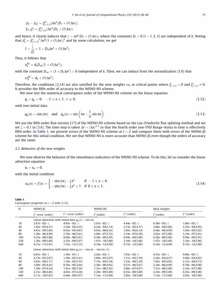
Table 1Converg

N

10204080160320640

10204080160320640


jb2 � b0j ¼ jf 000jþ1=2jDx3ðD1 þOðDxÞÞ;jL1;1f j ¼ jf 000jþ1=2jDx3ðD2 þOðDxÞÞ

and hence, it clearly induces that f ¼ Dx6ðD3 þOðDxÞÞ, where the constants Di > 0 (i ¼ 1;2;3) are independent of k. Notingthat b2

k ¼ jf 00jþ1=2j2Dx4ð1þOðDxÞÞ2 and by some calculation, we get

1þ f

b2k

¼ 1þ D4Dx2 þOðDx3Þ:

Thus, it follows that

aNSk ¼ dkDDxð1þOðDx3ÞÞ:

with the constant DDx ¼ ð1þ D3Dx2Þ > 0 independent of k. Then, we can induce from the normalization (3.9) that

xNSk ¼ dk þOðDx3Þ:

Therefore, the conditions (2.14) are also satisfied for the new weights xk at critical points where f 0jþ1=2 ¼ 0 and f 00jþ1=2 – 0.It provides the fifth-order of accuracy to the WENO-NS scheme.

We now test the numerical convergence order of the WENO-NS scheme on the linear equation

qt þ qx ¼ 0; �1 6 x 6 1; t P 0; ð3:12Þ

with two initial data

q0ðxÞ ¼ sinðpxÞ and q0ðxÞ ¼ sin px� 1p

sin px� �

: ð3:13Þ

We use the fifth-order flux-version [17] of the WENO-NS scheme based on the Lax–Friedrichs flux splitting method and weset n ¼ 0:1 in (3.6). The time step is taken Dt � ðDxÞ5=4 so that the fourth order non-TVD Runge–Kutta in time is effectivelyfifth-order. In Table 1, we present errors of the WENO-NS scheme at t ¼ 2 and compare them with errors of the WENO-JSscheme for this initial condition. We see that WENO-NS is more accurate than WENO-JS even though the orders of accuracyare the same.

3.3. Behaviors of the new weights

We now observe the behavior of the smoothness indicators of the WENO-NS scheme. To do this, let us consider the linearadvection equation

ut þ ux ¼ 0;

with the initial condition

u0ðxÞ ¼ f ðxÞ ¼� sinðpxÞ � 1

2 x3 if � 1 6 x < 0;� sinðpxÞ � 1

2 x3 þ 1 if 0 6 x 6 1;

(ð3:14Þ

ence properties at t ¼ 2 with (3.13).

WENO-JS WENO-NS Ideal weights

L1-error (order) L1-error (order) L1(order) L1(order) L1(order) L1(order)

Linear advection with initial data q0ðxÞ ¼ sinðpxÞ2.87e�02(–) 4.85e�02(–) 2.91e�02(–) 4.44e�02(–) 6.58e�03(–) 1.06e�02(–)1.45e�03(4.31) 2.54e�03(4.25) 8.24e�04(5.14) 2.15e�03(4.37) 2.06e�04(5.00) 3.33e�04(4.99)4.41e�05(5.04) 8.92e�05(4.83) 9.63e�06(6.42) 3.05e�05(6.14) 6.46e�06(4.99) 1.03e�05(5.02)1.38e�06(4.99) 2.78e�06(5.01) 2.09e�07(5.52) 3.19e�07(6.58) 2.02e�07(5.00) 3.19e�07(5.01)4.33e�08(5.00) 8.60e�08(5.01) 6.30e�09(5.05) 9.94e�09(5.00) 6.30e�09(5.00) 9.94e�09(5.01)1.36e�09(5.00) 2.55e�09(5.07) 1.97e�10(5.00) 3.10e�10(5.00) 1.97e�10(5.00) 3.10e�10(5.00)4.21e�11(5.01) 7.35e�11(5.12) 6.18e�12(4.99) 9.72e�12(5.00) 6.18e�12(4.99) 9.72e�12(5.00)

Linear advection with initial data q0ðxÞ ¼ sinðpx� sinðpxÞ=pÞ

6.01e�02(–) 1.36e�01(–) 2.42e�02(–) 7.93e�02(–) 4.35e�02(–) 9.06e�02(–)4.73e�03(3.67) 1.28e�02(3.41) 2.89e�03(3.07) 1.31e�02(2.59) 2.26e�03(4.27) 5.60e�03(4.02)3.62e�04(3.71) 1.10e�03(3.55) 7.15e�05(5.34) 3.33e�04(5.30) 7.45e�05(4.92) 2.12e�04(4.73)1.69e�05(4.42) 8.76e�05(3.64) 2.36e�06(4.92) 6.57e�06(5.67) 2.34e�06(4.99) 6.70e�06(4.98)7.30e�07(4.54) 7.41e�06(3.56) 7.31e�08(5.02) 2.09e�07(4.97) 7.31e�08(5.00) 2.10e�07(5.00)2.51e�08(4.86) 4.03e�07(4.20) 2.29e�09(5.00) 6.55e�09(5.00) 2.29e�09(5.00) 6.55e�09(5.00)5.11e�10(5.62) 6.44e�09(5.97) 7.14e�11(5.00) 2.05e�10(5.00) 7.14e�11(5.00) 2.05e�10(5.00)


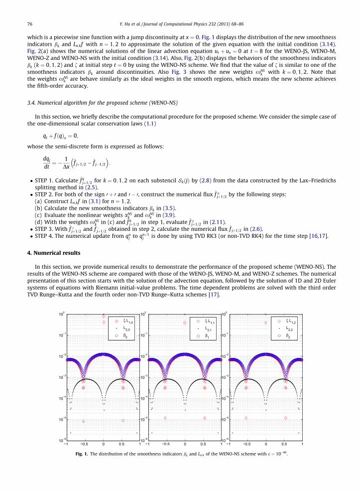
which is a piecewise sine function with a jump discontinuity at x ¼ 0. Fig. 1 displays the distribution of the new smoothnessindicators bk and Ln;kf with n ¼ 1;2 to approximate the solution of the given equation with the initial condition (3.14).Fig. 2(a) shows the numerical solutions of the linear advection equation ut þ ux ¼ 0 at t ¼ 8 for the WENO-JS, WENO-M,WENO-Z and WENO-NS with the initial condition (3.14). Also, Fig. 2(b) displays the behaviors of the smoothness indicatorsbk (k ¼ 0;1;2) and f at initial step t ¼ 0 by using the WENO-NS scheme. We find that the value of f is similar to one of thesmoothness indicators bk around discontinuities. Also Fig. 3 shows the new weights xNS

k with k ¼ 0;1;2. Note thatthe weights xNS

k are behave similarly as the ideal weights in the smooth regions, which means the new scheme achievesthe fifth-order accuracy.

3.4. Numerical algorithm for the proposed scheme (WENO-NS)

In this section, we briefly describe the computational procedure for the proposed scheme. We consider the simple case ofthe one-dimensional scalar conservation laws (1.1)

qt þ f ðqÞx ¼ 0;

whose the semi-discrete form is expressed as follows:

dqj

dt¼ � 1

Dxf̂ jþ1=2 � f̂ j�1=2

� :

STEP 1. Calculate f̂ kjþ1=2 for k ¼ 0;1;2 on each substencil SkðjÞ by (2.8) from the data constructed by the Lax–Friedrichs

splitting method in (2.5). STEP 2. For both of the sign 0 þ 0 and 0 � 0, construct the numerical flux f̂�jþ1=2 by the following steps:

(a) Construct Ln;kf in (3.1) for n ¼ 1;2.(b) Calculate the new smoothness indicators bk in (3.5).(c) Evaluate the nonlinear weights aNS

k and xNSk in (3.9).

(d) With the weights xNSk in (c) and f̂ k

jþ1=2 in step 1, evaluate f̂�jþ1=2 in (2.11). STEP 3. With f̂þjþ1=2 and f̂�jþ1=2 obtained in step 2, calculate the numerical flux f̂ jþ1=2 in (2.6). STEP 4. The numerical update from qn

j to qnþ1j is done by using TVD RK3 (or non-TVD RK4) for the time step [16,17].

4. Numerical results

In this section, we provide numerical results to demonstrate the performance of the proposed scheme (WENO-NS). Theresults of the WENO-NS scheme are compared with those of the WENO-JS, WENO-M, and WENO-Z schemes. The numericalpresentation of this section starts with the solution of the advection equation, followed by the solution of 1D and 2D Eulersystems of equations with Riemann initial-value problems. The time dependent problems are solved with the third orderTVD Runge–Kutta and the fourth order non-TVD Runge–Kutta schemes [17].

Fig. 1. The distribution of the smoothness indicators bk and Ln;k of the WENO-NS scheme with e ¼ 10�40.

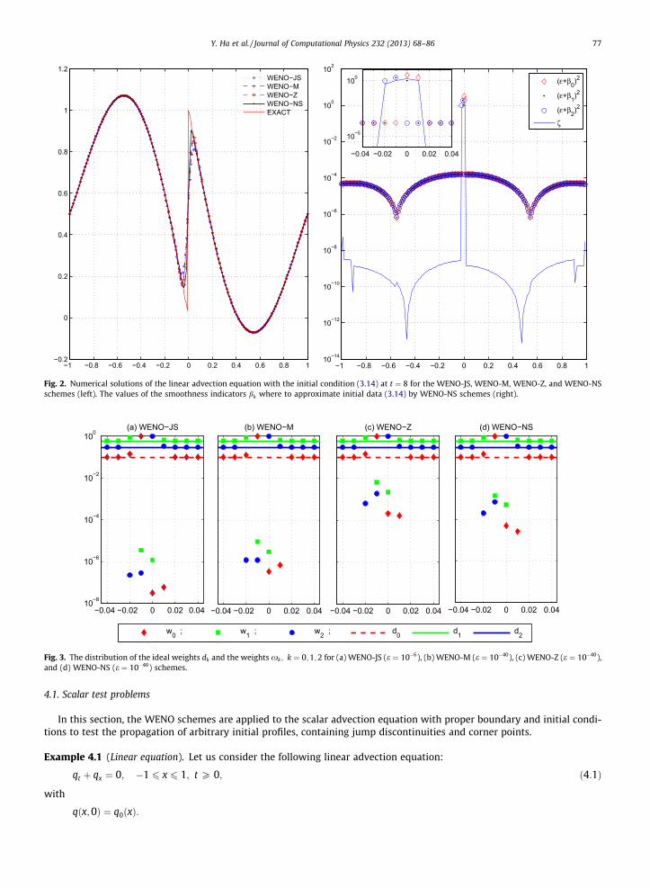
Fig. 2. Numerical solutions of the linear advection equation with the initial condition (3.14) at t ¼ 8 for the WENO-JS, WENO-M, WENO-Z, and WENO-NSschemes (left). The values of the smoothness indicators bk where to approximate initial data (3.14) by WENO-NS schemes (right).

Fig. 3. The distribution of the ideal weights dk and the weights xk; k ¼ 0;1;2 for (a) WENO-JS (e ¼ 10�6), (b) WENO-M (e ¼ 10�40), (c) WENO-Z (e ¼ 10�40),and (d) WENO-NS (e ¼ 10�40) schemes.


4.1. Scalar test problems

In this section, the WENO schemes are applied to the scalar advection equation with proper boundary and initial condi-tions to test the propagation of arbitrary initial profiles, containing jump discontinuities and corner points.

Example 4.1 (Linear equation). Let us consider the following linear advection equation:

qt þ qx ¼ 0; �1 6 x 6 1; t P 0; ð4:1Þ

with

qðx;0Þ ¼ q0ðxÞ:


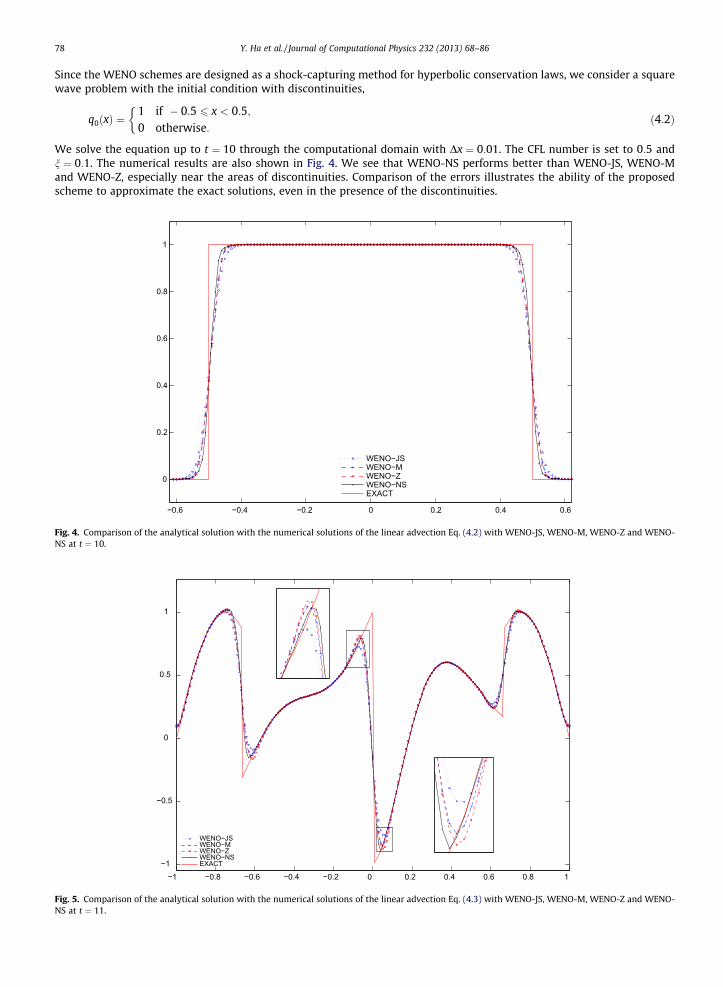
Since the WENO schemes are designed as a shock-capturing method for hyperbolic conservation laws, we consider a squarewave problem with the initial condition with discontinuities,

Fig. 4.NS at t

Fig. 5.NS at t

q0ðxÞ ¼1 if � 0:5 6 x < 0:5;0 otherwise:

�ð4:2Þ

We solve the equation up to t ¼ 10 through the computational domain with Dx ¼ 0:01. The CFL number is set to 0:5 andn ¼ 0:1. The numerical results are also shown in Fig. 4. We see that WENO-NS performs better than WENO-JS, WENO-Mand WENO-Z, especially near the areas of discontinuities. Comparison of the errors illustrates the ability of the proposedscheme to approximate the exact solutions, even in the presence of the discontinuities.

−0.6 −0.4 −0.2 0 0.2 0.4 0.6

0

0.2

0.4

0.6

0.8

1

WENO−JSWENO−MWENO−ZWENO−NSEXACT

Comparison of the analytical solution with the numerical solutions of the linear advection Eq. (4.2) with WENO-JS, WENO-M, WENO-Z and WENO-¼ 10.

−1 −0.8 −0.6 −0.4 −0.2 0 0.2 0.4 0.6 0.8 1−1

−0.5

0

0.5

1


Comparison of the analytical solution with the numerical solutions of the linear advection Eq. (4.3) with WENO-JS, WENO-M, WENO-Z and WENO-¼ 11.


Moreover, we solve the linear advection Eq. (4.1) with the following initial condition,

Fig. 6.and 401

q0ðxÞ ¼�x sinð3p

2 x2Þ; if � 1 6 x 6 � 13 ;

j sinð2pxÞj; if � 13 < x 6 1

3 ;

2x� 1� 16 sinð3pxÞ; if 1

3 6 x 6 1:

8><>: ð4:3Þ

The solution of this equation consists of contact discontinuities, corner singularities and smooth areas. We solve the equationup to t ¼ 11 through the computational domain. The CFL number is set to 0:5. The numerical results are also shown in Fig. 5.WENO-NS performs better than WENO-JS, WENO-M and WENO-Z, especially near the areas of discontinuities. Comparison ofthe errors illustrates the ability of the proposed scheme to approximate the exact solutions, even in the presence of thediscontinuities.

4.2. 1D Euler systems

In this section, we present the numerical results for the hyperbolic systems of conservation laws of the form (1.1) withm > 1. The tests are performed on the system of the 1D Euler equation:

Ut þ FðUÞx ¼ 0; ð4:4Þ

with

U ¼ ðq;qu; EÞT ; FðUÞ ¼ qu;qu2 þ p;uðEþ pÞ� �T

:

−5 −4 −3 −2 −1 0 1 2 3 4 5

1

1.5

2

2.5

3

3.5

4

4.5 WENO−JSWENO−MWENO−ZWENO−NSEXACT

−5 −4 −3 −2 −1 0 1 2 3 4 5

1

1.5

2

2.5

3

3.5

4

4.5 WENO−JSWENO−MWENO−ZWENO−NSEXACT

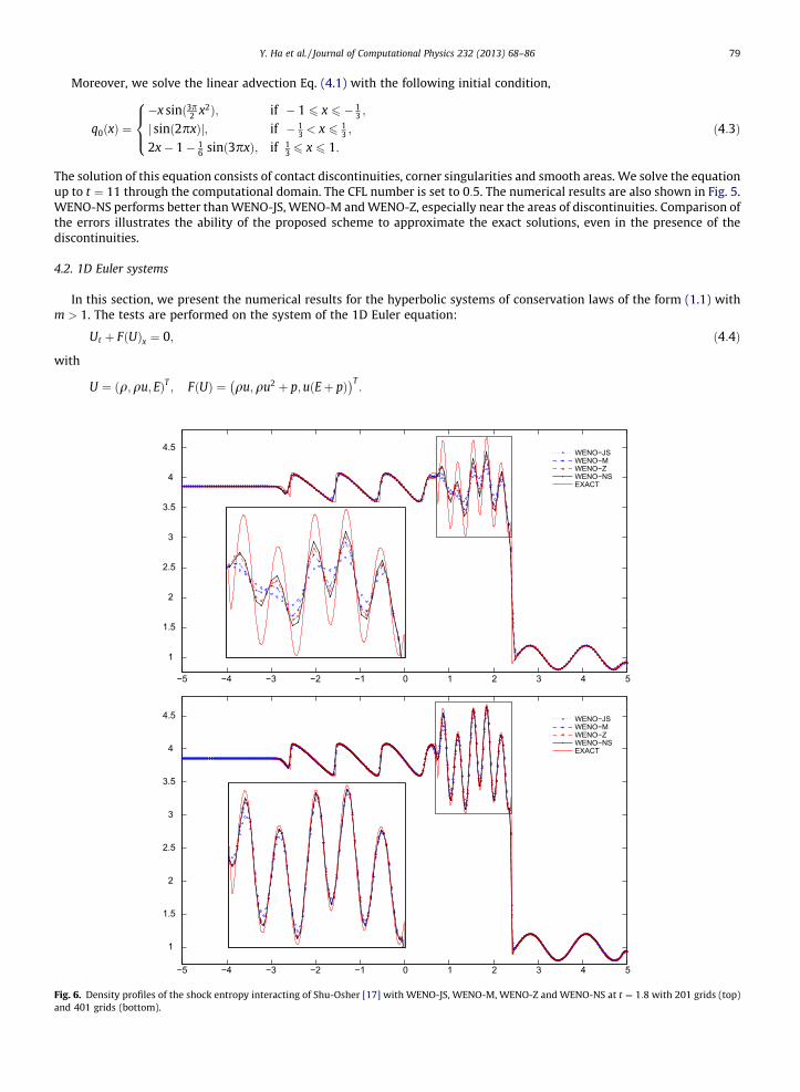
Density profiles of the shock entropy interacting of Shu-Osher [17] with WENO-JS, WENO-M, WENO-Z and WENO-NS at t ¼ 1:8 with 201 grids (top)grids (bottom).


The equation of state is given by

Fig. 7.density

Fig. 8.density

p ¼ ðc� 1Þ E� 12qu2

� �;

where q; u; p and E are the density, velocity, pressure and total energy respectively, and where c is the ratio of specific heats.The eigenvalues of the Jacobian matrix AðUÞ ¼ @F=@U are

−5 −4 −3 −2 −1 0 1 2 3 4 5

0.4

0.5

0.6

0.7

0.8

0.9

1

1.1

1.2

1.3(a)

−5 −4 −3 −2 −1 0 1 2 3 4 50.511.522.533.5(b)


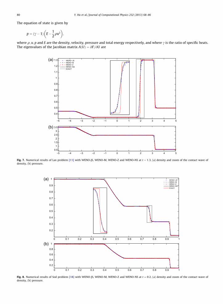
Numerical results of Lax problem [11] with WENO-JS, WENO-M, WENO-Z and WENO-NS at t ¼ 1:3, (a) density and zoom of the contact wave of, (b) pressure.

0 0.1 0.2 0.3 0.4 0.5 0.6 0.7 0.8 0.9 1

0.2

0.3

0.4

0.5

0.6

0.7

0.8

0.9

1(a)

(b)

0 0.1 0.2 0.3 0.4 0.5 0.6 0.7 0.8 0.9 1

0.2

0.4

0.6

0.8

1


Numerical results of Sod problem [18] with WENO-JS, WENO-M, WENO-Z and WENO-NS at t ¼ 0:2, (a) density and zoom of the contact wave of, (b) pressure.

(a)

0.

0.

0.

0.

0.

0.

0.

0.

0.

(c)

0.

0.

0.

0.

0.

0.

0.

0.

0.


a1ðqÞ ¼ u� c; a2ðqÞ ¼ u; a3ðqÞ ¼ uþ c;

where c ¼ ðcp=qÞ1=2 is the sound speed. The characteristic decomposition is chosen to generalize the WENO schemes to 1DEuler systems [16]. In the following examples in 1D Euler systems, we set n ¼ 0:4 in (3.6).

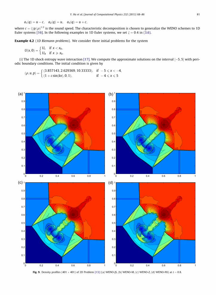
Example 4.2 (1D Riemann problems). We consider three initial problems for the system

Uðx;0Þ ¼UL if x < x0;

UR if x P x0:

�

(i) The 1D shock entropy wave interaction [17]. We compute the approximate solutions on the interval ½�5;5� with peri-odic boundary conditions. The initial condition is given by

ðq;u;pÞ ¼ð3:857143;2:629369;10:33333Þ; if � 5 6 x < �4;ð1þ e sinðkxÞ; 0;1Þ; if � 4 6 x 6 5

�

0 0.2 0.4 0.6 0.8 10

1

2

3

4

5

6

7

8

9

1 (b)

0 0.2 0.4 0.6 0.8 10

0.1

0.2

0.3

0.4

0.5

0.6

0.7

0.8

0.9

1

0 0.2 0.4 0.6 0.8 10

1

2

3

4

5

6

7

8

9

1 (d)

0 0.2 0.4 0.6 0.8 10

0.1

0.2

0.3

0.4

0.5

0.6

0.7

0.8

0.9

1

Fig. 9. Density profiles (401 401) of 2D Problem [13] ((a) WENO-JS, (b) WENO-M, (c) WENO-Z, (d) WENO-NS) at t ¼ 0:8.


where e and k are the amplitude and wave number of the entropy wave, respectively. Here, we set e ¼ 0:2 and k ¼ 5. In thisproblem, a right-moving supersonic (Mach 3) shock wave interacts with sine waves in a density disturbance that generates aflow field with both smooth structures and discontinuities. This flow induces wave trails behind a right-going shock at wavenumbers higher than the initial density-variation wave number k. Since the exact solution is unknown, the reference solu-tion (which can be regarded as the exact solutions) is obtained by using the fifth-order WENO-JS scheme [10] with 3201 gridpoints. The initial condition contains a jump discontinuity at x ¼ �4 and especially, the initial density profile has oscillationson ½�4;5�. Fig. 6 compares the numerical results for density profiles with the exact solutions. We solve the equation up tot ¼ 1:8 with Dx ¼ 0:04 and Dx ¼ 0:02 respectively. The CFL number is set to 0:5. Since the velocity and pressure profilesare not explanatory as density, we do not show them in this paper. WENO-NS captures shocks better than WENO-JS, espe-cially at the high-frequency waves behind the right going shock, providing high-resolution images and resolving all local ex-trema accurately. The WENO-NS scheme performs better than the WENO-JS, WENO-M and WENO-Z schemes.

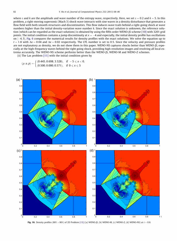
(ii) The Lax problem [11] with the initial condition given by

(a)

0

0

0

0

0

0

0

0

0

(c)

0

0

0

0

0

0

0

0

0

ðq;u;pÞ ¼ð0:445; 0:698;3:528Þ; if � 5 6 x < 0;ð0:500; 0:000; 0:571Þ; if 0 6 x 6 5

�

0 0.2 0.4 0.6 0.8 10

.1

.2

.3

.4

.5

.6

.7

.8

.9

1 (b)

0 0.2 0.4 0.6 0.8 10

0.1

0.2

0.3

0.4

0.5

0.6

0.7

0.8

0.9

1

0 0.2 0.4 0.6 0.8 10

.1

.2

.3

.4

.5

.6

.7

.8

.9

1 (d)

0 0.2 0.4 0.6 0.8 10

0.1

0.2

0.3

0.4

0.5

0.6

0.7

0.8

0.9

1

Fig. 10. Density profiles (801 801) of 2D Problem [13] ((a) WENO-JS, (b) WENO-M, (c) WENO-Z, (d) WENO-NS) at t ¼ 0:8.


with c ¼ 1:4. We solve the equation up to t ¼ 1:3 with Dx ¼ 0:05. The CFL number is set to 0:5. The numerical results for thedensity and pressure field are displayed in Fig. 7. The proposed method performs better than WENO-JS, WENO-M andWENO-Z. Here, we use the exact Riemann solver reported in Toro [19].

(iii) The Sod problem [18] with the initial condition given by

Fig. 11.bottom

ðq;u;pÞ ¼ð1:000;0:750;1:000Þ if 0 6 x < 0:5;ð0:125;0:000;0:100Þ if 0:5 6 x 6 1;

�

with c ¼ 1:4. We solve the equation up to t ¼ 0:2 with Dx ¼ 0:005. The CFL number is set to 0:5. The numerical results of thedensity and pressure field are displayed in Fig. 8. WENO-NS performs better than WENO-JS but yields similar result asWENO-M and WENO-Z. We use the exact Riemann solver reported in Toro [19].

4.3. 2D Euler systems

In this subsection we extend the WENO-NS scheme to solve the 2D compressible Euler systems of the form:

Ut þ FðUÞx þ GðUÞy ¼ 0; ð4:5Þ

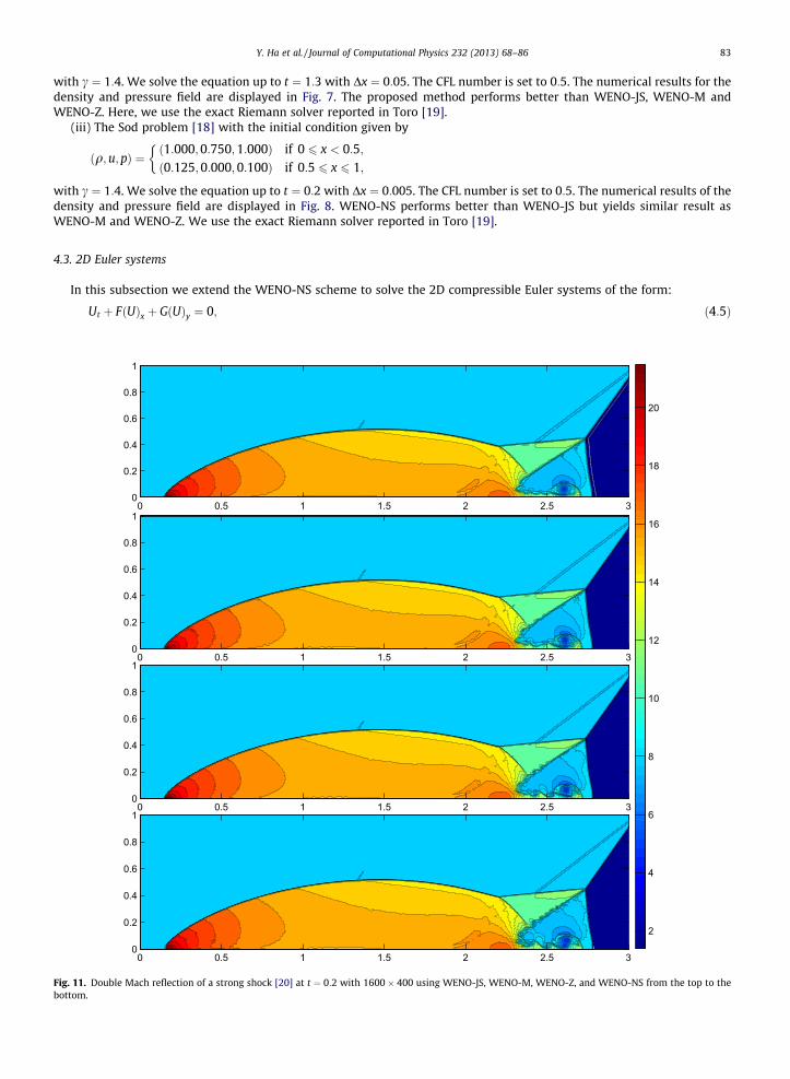
0 0.5 1 1.5 2 2.5 30

0.2

0.4

0.6

0.8

1

0 0.5 1 1.5 2 2.5 30

0.2

0.4

0.6

0.8

1

0 0.5 1 1.5 2 2.5 30

0.2

0.4

0.6

0.8

1

0 0.5 1 1.5 2 2.5 30

0.2

0.4

0.6

0.8

1

2

4

6

8

10

12

14

16

18

20

Double Mach reflection of a strong shock [20] at t ¼ 0:2 with 1600 400 using WENO-JS, WENO-M, WENO-Z, and WENO-NS from the top to the.

2 2.2 2.4 2.6 2.80

0.1

0.2

0.3

0.4

0.5

2 2.2 2.4 2.6 2.80

0.1

0.2

0.3

0.4

0.5

2 2.2 2.4 2.6 2.80

0.1

0.2

0.3

0.4

0.5

0.6

2 2.2 2.4 2.6 2.80

0.1

0.2

0.3

0.4

0.5

0.6

2 2.2 2.4 2.6 2.80

0.1

0.2

0.3

0.4

0.5

2 2.2 2.4 2.6 2.80

0.1

0.2

0.3

0.4

0.5

2 2.2 2.4 2.6 2.80

0.1

0.2

0.3

0.4

0.5

0.6

2 2.2 2.4 2.6 2.80

0.1

0.2

0.3

0.4

0.5

0.6

2 2.2 2.4 2.6 2.80

0.1

0.2

0.3

0.4

0.5

2 2.2 2.4 2.6 2.80

0.1

0.2

0.3

0.4

0.5

2 2.2 2.4 2.6 2.80

0.1

0.2

0.3

0.4

0.5

0.6

2 2.2 2.4 2.6 2.80

0.1

0.2

0.3

0.4

0.5

0.6

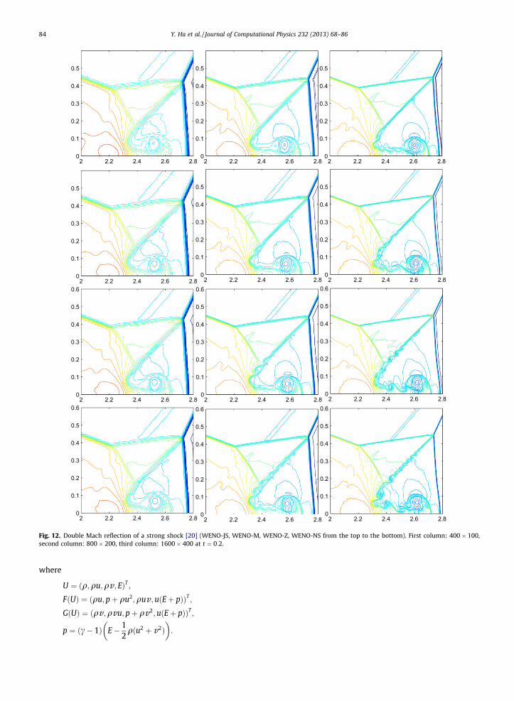
Fig. 12. Double Mach reflection of a strong shock [20] (WENO-JS, WENO-M, WENO-Z, WENO-NS from the top to the bottom). First column: 400 100,second column: 800 200, third column: 1600 400 at t ¼ 0:2.


where

U ¼ ðq;qu;qv ; EÞT ;FðUÞ ¼ ðqu;pþ qu2;quv ;uðEþ pÞÞT ;GðUÞ ¼ ðqv ;qvu; pþ qv2;uðEþ pÞÞT ;

p ¼ ðc� 1Þ E� 12qðu2 þ v2Þ

� �:


Here q; u; v ; p and E are density, components of velocity in the x and y coordinate directions, pressure and total energy,respectively. Also, U is the vector of conservative variables, FðUÞ the x-wise-flux component, and GðUÞ the y-wise-flux com-ponent. The proposed method is applied dimension-by-dimension to solve the 2D compressible Euler systems.

Example 4.3 (2D Problem for 2D gas dynamics). We consider numerical solutions of the 2D Riemann problems proposed by[13]. This problem is solved on the square ½0;1� ½0;1�. The square is divided into four quadrants by lines x ¼ 0:8 and y ¼ 0:8.We define the initial data as constant states on each of four quadrants and evolve this initial data until time t ¼ 0:8 with CFL= 0.5. The Riemann problems are defined by initial constant states in each quadrant:

ðq;u;v ;pÞ ¼

ð1:5;0;0;1:5Þ if 0:8 6 x 6 1; 0:8 6 y 6 1;ð0:5323;1:206;0; 0:3Þ if 0 6 x < 0:8; 0:8 6 y 6 1;ð0:138;1:206;1:206;0:029Þ if 0 6 x < 0:8; 0 6 y < 0:8;ð0:5323;0;1:206; 0:3Þ if 0:8 < x 6 1; 0 6 y < 0:8:

8>>><>>>:

We set the gas constant c ¼ 1:4. To the best of our knowledge, the exact solution has not been elucidated for this 2D prob-lem. We compare the numerical performance of the WENO-NS scheme with WENO-JS, WENO-M, and WENO-Z in Figs. 9 and10. An examination of these results reveals that WENO-NS (d) displays a better resolution of the structure appearing in otherWENO schemes.

Example 4.4 (Double Mach reflection of a strong shock). Finally, we apply our scheme to the two dimensional double-Machshock reflection problem [20] where a vertical shock wave moves horizontally into a wedge that is inclined by some angle.The computation domain for this problem is chosen to be ½0;4� ½0;1�, and the reflecting wall lies at the bottom of thecomputational domain for 1

6 6 x 6 4. Initially a right-moving Mach 10 shock is positioned at x ¼ 16 ; y ¼ 0, and makes a 60�

angle with the x-axis. For the bottom boundary, the exact postshock condition is imposed for the part from x ¼ 0 to x ¼ 16 and

a reflective boundary condition is used for the rest. The top boundary of our computational domain uses the exact motion ofthe Mach 10 shock. Inflow and outflow boundary conditions are used for the left and right boundaries. The unshocked fluidhas a density of 1:4 and a pressure of 1. The problem was run till t ¼ 0:2 and the blow-up region around the double Machstems. The ratio of specific heats c ¼ 1:4. We set the CFL number as 0:5. The results in ½0;3� ½0;1� are displayed. Wecompare the numerical performance of the WENO-NS scheme with WENO-JS in Fig. 11. The (contours) zoomed around thedouble Mach reflection region are given in Fig. 12. We can clearly see that the contact discontinuity resolution (manifestedby the small scale structures) is improved by WENO-NS to WENO-JS. We can see that most of the flow features are capturedwell by WENO-NS.

5. Conclusion

In this paper, we introduce the modified smoothness indicators of WENO schemes (WENO-NS) for the approximate solu-tion of nonlinear hyperbolic conservation laws. In a number of numerical experiments, one- and two-dimensional scalar andsystem cases are considered and the proposed schemes exhibit excellent performances in all test cases. Comparisons be-tween WENO-NS and other fifth-order WENO schemes reveal clear advantages on approximating near the discontinuities.Numerical experiments show that WENO-NS schemes resolve discontinuities sharply while keeping an essential non-oscil-latory performance. The improvement is attributed to the ability of WENO-NS to detect the complicated solution structures.

6. Appendix: proof of Theorem 3.2

For the given function f 2 C3ðIÞ, let us write f ¼ Tjf þ Rjf with Tjf the second degree Taylor polynomial of f around xjþ1=2,that is,

Tjf ðxÞ :¼X2

m¼0

ðx� xjþ1=2Þmdmfdxm ðxjþ1=2Þ=m! ð6:1Þ

and Rjf its remainder. Then, applying the condition (3.2), it is immediate that

Xx‘2SkðjÞ

c½n�k;‘Tjf ðx‘Þ ¼X2

m¼0

dmfdxm ðxjþ1=2Þ

Xx‘2SkðjÞ

c½n�k;‘ðx‘ � xjþ1=2Þm=m! ¼ dnfdxn ðxjþ1=2Þ

Xx‘2SkðjÞ

c½n�k;‘ðx‘ � xjþ1=2Þn=n! ¼ dnfdxn ðxjþ1=2ÞDxn:

Apparently, it follows that

Ln;kf ¼X

x‘2SkðjÞc½n�k;‘ðTjf ðx‘Þ þ Rjf ðx‘ÞÞ ¼

dnfdxn ðxjþ1=2ÞDxn þ

Xx‘2SkðjÞ

c½n�k;‘Rjf ðx‘Þ: ð6:2Þ


Here, since the given set SkðjÞ is uniform, say, SkðjÞ :¼ fxn ¼ x0 þ nDx j n ¼ jþ k� 2; . . . ; jþ kg, then the linear system in (3.3)is changed to

M1 � c½n�k ¼ r1; ð6:3Þ

with the matrices M and r of the form

M1 :¼Mk :¼ kþ ‘� 52

� �m

=m! : ‘; m ¼ 0;1;2� �

r1 :¼ rn :¼ ðdn;m : m ¼ 0;1;2ÞT ;

which are independent of the evaluation point xjþ1=2 and the density Dx. Thus, it is obvious that the coefficients c½n�k;‘ are uni-formly bounded by a constant which is independent of Dx; k and n. Moreover, since Rjf is the remainder of the Taylor poly-nomial Tjf , the explicit formula of Rjf induces the bound

jRjf ðx‘Þj 6 cDx3; x‘ 2 SkðjÞ;

with a constant c > 0 independent of x‘ 2 SkðjÞ, xjþ1=2 and Dx. Thus, combining this bound with (6.2), the proof is completed.

Acknowledgements

The authors are very grateful to the anonymous referee for the valuable suggestion on this paper. This work was sup-ported by Basic Science Research Program 2010–0011689 (Y. Lee) and Priority Research Centers Program 2011–0022979(Y. Lee, J. Yoon), through the National Research Foundation of Korea (NRF) funded by the Ministry of Education, Scienceand Technology.

References

[1] D.S. Balsara, C.W. Shu, Monotonicity preserving WENO schemes with increasingly high-order of accuracy, J. Comput. Phys. 160 (2000) 405–452.[2] R. Borges, M. Carmona, B. Costa, W.S. Don, An improved WENO scheme for hyperbolic conservation laws, J. Comput. Phys. 227 (2008) 3191–3211.[3] M. Castro, B. Costa, W.S. Don, High order weighted essentially non-oscillatory WENO-Z schemes for hyperbolic conservation laws, J. Comput. Phys. 230

(2011) 1766–1792.[4] G.A. Gerolymos, D. Sénéchal, I. Vallet, Very-high-order WENO schemes, J. Comput. Phys. 228 (2009) 8481–8524.[5] A. Harten, High resolution schemes for hyperbolic conservation laws, J. Comput. Phys. 49 (1983) 357–393.[7] A. Harten, S. Osher, Uniformly high-order accurate non-oscillatory schemes I, SIAM J. Numer. Anal. 24 (2) (1987) 279–309.[8] A. Harten, B. Engquist, S. Osher, S. Chakravarthy, Uniformly high-order accurate non-oscillatory schemes III, J. Comput. Phys. 71 (1987) 231–303.[9] A.K. Henrick, T.D. Aslam, J.M. Powers, Mapped weighted-essentially-non-oscillatory schemes: achieving optimal order near critical points, J. Comput.

Phys. 207 (2005) 542–567.[10] G. Jiang, C.W. Shu, Efficient implementation of weighted ENO schemes, J. Comput. Phys. 126 (1996) 202–228.

[11] P.D. Lax, Weak solutions of nonlinear hyperbolic equations and their numerical computation, Commun. Pure Appl. Math. 7 (1954) 159–193.[12] X.-D. Liu, S. Osher, T. Chan, Weighted essentially non-oscillatory schemes, J. Comput. Phys. 115 (1994) 200–212.[13] C.W. Schulz-Rinne, J.P. Collins, H.M. Glaz, Numerical solution of the Riemann problem for two-dimensional gas dynamics, SIAM J. Sci. Comput. 14 (6)

(1993) 1394–1414.[14] S. Serna, A. Marquina, Power-ENO methods: a fifth-order accurate weighted power ENO method, J. Comput. Phys. 194 (2004) 632–658.[15] C.W. Shu, Essentially non-oscillatory and weighted essentially non-oscillatory schemes for hyperbolic conservation laws, in: A. Quarteroni (Ed.),

Advanced Numerical Approximation of Nonlinear Hyperbolic Equations, Lecture Notes in Mathematics, vol. 1697, Springer-Verlag, Berlin/New York,1998, pp. 325–432.

[16] C.W. Shu, S. Osher, Efficient implementation of essentially non-oscillatory shock capturing schemes, J. Comput. Phys. 77 (1988) 439–471.[17] C.W. Shu, S. Osher, Efficient implementation of essentially non-oscillatory shock capturing schemes II, J. Comput. Phys. 83 (1989) 32–78.[18] G. Sod, A survey of several finite difference methods for systems of nonlinear hyperbolic conservation laws, J. Comput. Phys. 27 (1978) 1–31.[19] E.F. Toro, Riemann Solvers and Numerical Methods for Fluid Dynamics, Springer-Verlag, New York, 1997.[20] P. Woodward, P. Colella, The numerical simulation of two-dimensional fluid flow with strong shocks, J. Comput. Phys. 54 (1984) 115–173.

an improved weighted essentially non-oscillatory scheme with a new smoothness indicator

Documents